On the connection between global centers and global injectivity in the plane

Abstract.

In this note we present a generalization of a result of Sabatini relating global injectivity and global centers. The shape of the image of the map is taking into account. Our proofs do not use Hadamard’s theorem.

1. Introduction and statement of the main results

Throughout our exposition $U\subset\mathbb{R}^{2}$ will be an open connected set.

Let $X,Y:U\to\mathbb{R}$ be $C^{k}$ functions for some $k\in\mathbb{N}$. We consider the vector field $\mathcal{X}=(X,Y)$, or equivalently the system of differential equations

(1) $$\dot{x}=X(x,y),\ \ \ \ \dot{y}=Y(x,y).$$

Let $z_{0}$ be an isolated singular point of system (1). We say that $z_{0}$ is a center of (1) when there exists a neighborhood $V$ of $z_{0}$, $V\subset U$, such that each orbit of (1) in $V\backslash\{z_{0}\}$ is periodic. We define the period annulus of center $z_{0}$, denoting it by $\mathcal{P}_{z_{0}}$, as the maximal open connected set $W\subset U$ such that $W\setminus\{z_{0}\}$ is filled with periodic orbits of $\mathcal{X}$. We say that the center is global when $\mathcal{P}_{z_{0}}=U$. We say that the center is isochronous when the orbits in $\mathcal{P}_{z_{0}}$ have the same period.

When the singular point $z_{0}$ is non-degenerate, i.e. the determinant of the linear part of $\mathcal{X}$ in $z_{0}$ is different from zero, in order to have a center it is necessary that the eingenvalues of $D\mathcal{X}(z_{0})$ are purely imaginary. In this case we will say that the center $z_{0}$ is non-degenerate.

Let $H:U\to\mathbb{R}$ be a $C^{k+1}$ function. We say that $H$ is the Hamiltonian of system (1) if

$$X(x,y)=-H_{y}(x,y),\ \ \ \ Y(x,y)=H_{x}(x,y).$$

In this case we call system (1) the Hamiltonian system associated to the Hamiltonian $H$. We also denote $\mathcal{X}=\nabla H^{\perp}$.

The following result provides a simple way to produce non-degenerate Hamiltonian centers. Let $f=(f_{1},f_{2}):U\to\mathbb{R}^{2}$. We denote by $H_{f}:U\to\mathbb{R}$ the Hamiltonian defined by

(2) $$H_{f}(x,y)=\frac{f_{1}(x,y)^{2}+f_{2}(x,y)^{2}}{2},$$

for each $(x,y)\in U$.

Lemma 1.

Let $f=(f_{1},f_{2}):U\to\mathbb{R}^{2}$ be a $C^{2}$ map. If $z_{0}\in U$ is such that $\det Df(z_{0})\neq 0$, then $z_{0}$ is a singular point of the Hamiltonian vector field $\nabla H_{f}^{\perp}$ if and only if $f(z_{0})=(0,0)$. In this case, this singular point $z_{0}$ is a non-degenerate center of $\nabla H_{f}^{\perp}$ and also an isolated global minimum of $H_{f}$. In particular, if

(3) $$\det Df={f_{1}}_{x}{f_{2}}_{y}-{f_{2}}_{x}{f_{1}}_{y}\neq 0$$

in $U$, then the singular points of $\nabla H_{f}^{\perp}$ are non-degenerate centers and correspond to the zeros of $f$.

In case the Jacobian determinant of $f$ in $U$ is a non-zero constant, it follows that the center $z_{0}$ is isochronous, see Theorem 2.1 of [9]. See also Theorem B of [8] for the characterization of the analytic Hamiltonian isochronous centers as being the ones such that locally the Hamiltonian has the form $H_{f}$, with $f$ having non-zero constant Jacobian determinant.

When $f:\mathbb{R}^{2}\to\mathbb{R}^{2}$ is a polynomial map satisfying (3) and such that $f(0,0)=(0,0)$, Sabatini proved in [9] that $f$ is a global diffeomorphism if and only if the center $(0,0)$ of $\nabla H_{f}^{\perp}$ is global. See an application of this result to the real Jacobian conjecture in [2]. The connection between injectivity of maps and centers also appears in [10], where there are results relating the injectivity of $C^{2}$ maps $f:\mathbb{R}^{2}\to\mathbb{R}^{2}$ having non-zero constant Jacobian determinant to the area of the period annulus of a center of $\nabla H_{f}^{\perp}$. In the same paper [10], the injectivity of $f$ is also related to the property that some vector fields other than $\nabla H_{f}^{\perp}$ are complete, without assuming that the Jacobian determinant of $f$ is constant. In [7] Gavrilov studied a connection between centers and injectivity in the complex context.

The main aim of this note is the following extension of some of the above-mentioned results for $C^{2}$ maps defined in connected open sets of $\mathbb{R}^{2}$.

Theorem 2.

Let $f:U\to\mathbb{R}^{2}$ be a $C^{2}$ map satisfying (3) and $z_{0}\in U$ such that $f(z_{0})=(0,0)$. The center $z_{0}$ of the Hamiltonian vector field $\nabla H_{f}^{\perp}$ is global if and only if (i) $f$ is injective and (ii) $f(U)=\mathbb{R}^{2}$ or $f(U)$ is an open disc centered at $(0,0)$.

In case $f:\mathbb{R}^{2}\to\mathbb{R}^{2}$ is a polynomial injective map, it follows that $f\left(\mathbb{R}^{2}\right)=\mathbb{R}^{2}$, see for instance [1]. Therefore our Theorem 2 generalizes the above-mentioned result of [9].

Corollary 3.

Let $f:U\to\mathbb{R}^{2}$ be a $C^{2}$ map satisfying (3) and $z_{0}\in U$ such that $f(z_{0})=(0,0)$. Then (i) $f$ is injective in $\overline{\mathcal{P}_{z_{0}}}$, where $\overline{\mathcal{P}_{z_{0}}}$ is the closure of $\mathcal{P}_{z_{0}}$ in $U$, and (ii) $f\left(\mathcal{P}_{z_{0}}\right)=\mathbb{R}^{2}$ or $f\left(\mathcal{P}_{z_{0}}\right)$ is an open disc centered at $(0,0)$.

In case $U=\mathbb{R}^{2}$ and the Jacobian determinant of $f$ is $1$, the statement (i) of Corollary 3 already appeared in [9] as Corollary 2.2.

The following estimates the size of the period annulus $\mathcal{P}_{z_{0}}$.

Corollary 4.

Let $f:U\to\mathbb{R}^{2}$ be a $C^{2}$ map satisfying (3) and $z_{0}\in U$ such that $f(z_{0})=(0,0)$. Then $\mathcal{P}_{z_{0}}$ is the greatest open connected set containing $z_{0}$ such that (i) $f$ is injective in it and (ii) its image under $f$ is $\mathbb{R}^{2}$ or an open disc centered at $(0,0)$.

We observe that in our proofs it is not possible to use the classical Hadamard result of global invertibility of maps, that a local diffeomorphism $F:B\to B$, where $B$ is a Banach space, is a global one if and only if $F$ is proper. This is because our domain is just an open connected set, and our maps can be not surjective.

We prove the results in section 2 and present examples to them in section 3. We also study the special case where $H_{f}$ is polynomial in section 4.

2. Proof of the results

Proof of Lemma 1.

Observe that $\nabla H_{f}^{\perp}(z_{0})=(0,0)$ is equivalent to $Df(z_{0})f(z_{0})=(0,0)$. Since $Df(z_{0})$ is invertible, it follows that $z_{0}$ is a singular point of $\nabla H_{f}^{\perp}$ if and only it is a zero of $f$.

Assume so that $f(z_{0})=(0,0)$. Since $f$ is locally injective, it follows that $f(z)\neq(0,0)$ for $z$ close enough to $z_{0}$, and so $z_{0}$ is an isolated global minimum of $H_{f}=\left(f_{1}^{2}+f_{2}^{2}\right)/2$.

The linear part of $\nabla H_{f}^{\perp}$ in $z_{0}$ is

$$D\nabla H_{f}^{\perp}(z_{0})=\left(\begin{array}[]{cc}-{f_{1}}_{x}{f_{1}}_{y}-{f_{2}}_{x}{f_{2}}_{y}&-{f_{1}}_{y}^{2}-{f_{2}}_{y}^{2}\\ {f_{1}}_{x}^{2}+{f_{2}}_{x}^{2}&{f_{1}}_{x}{f_{1}}_{y}+{f_{2}}_{x}{f_{2}}_{y}.\end{array}\right).$$

Since $\det\left(D\nabla H_{f}^{\perp}\right)=\left(\det Df\right)^{2}>0$, we conclude that $z_{0}$ is a non-degenerate singularity and that the eigenvalues of $D\nabla H_{f}^{\perp}(z_{0})$ are purely imaginary, because $\textnormal{tr}\left(D\nabla H_{f}^{\perp}\right)=0$. Since the orbits of $\nabla H_{f}^{\perp}$ are contained in the level sets of $H_{f}$, and $z_{0}$ is an isolated minimum of $H_{f}$, we conclude that $z_{0}$ is a center of this vector field. ∎

The proof of Theorem 2 is a straightforward consequence of the following two lemmas.

Lemma 5.

Let $f:U\to\mathbb{R}^{2}$ be an injective $C^{2}$ map satisfying (3) and $z_{0}\in U$ be such that $f(z_{0})=(0,0)$. The center $z_{0}$ of the Hamiltonian vector field $\nabla H_{f}^{\perp}$ is global if and only if $f(U)=\mathbb{R}^{2}$ or $f(U)$ is an open disc centered at $(0,0)$.

Proof.

From hypothesis and from Lemma 1, the only singular point of $\nabla H_{f}^{\perp}$ is $z_{0}$. Thus from the definition of $H_{f}$ in (2) we see that $z_{0}$ is the only point in the level set $H_{f}^{-1}\{0\}$, hence the non-singular orbits of $\nabla H_{f}^{\perp}$ are the connected components of the level sets of $H_{f}^{-1}\{h\}$ for $h>0$, $h\in H_{f}(U)$. Clearly $h\in H_{f}(U)$ if and only if the circle

$$S_{h}=\left\{\sqrt{2h}e^{i\theta}\ |\ \theta\in\mathbb{R}\right\}$$

intersects $f(U)$.

Assume that $f(U)$ is $\mathbb{R}^{2}$ or a ball centered at $0$. Then $h\in H_{f}(U)$ if and only if $S_{h}\subset f(U)$. Therefore $H_{f}^{-1}\{h\}$ is the image of $S_{h}$ by $f^{-1}$. Thus $H_{f}^{-1}\{h\}$ is a topological circle. This proves that the non-singular orbits of $\nabla H_{f}^{\perp}$ are periodic. Hence the center $z_{0}$ is global.

On the other hand, assume that the center $z_{0}$ is global. Let $y\in f(U)$, $y\neq(0,0)$, and set $h_{y}=H_{f}(f^{-1}(y))$. Since the orbits of $\nabla H_{f}^{\perp}$ are periodic, it follows that the connected components of $H_{f}^{-1}\{h_{y}\}$ are topological circles. Hence the image of each of them by $f$ is a topological circle contained in $S_{h_{y}}$. Therefore each image is the circle $S_{h_{y}}$ (and hence $H_{f}^{-1}\{h_{y}\}$ is connected). In particular, $S_{h_{y}}\subset f(U)$. Then we have just proved that for each $y\in f(U)$, the circle $S_{h_{y}}$ containing $y$ is contained in $f(U)$. As a consequence

$$f(U)=\{(0,0)\}\cup\bigcup_{h\in H_{f}(U)}S_{h}.$$

The set $H_{f}(U)$ is an interval of the form $[0,\ell)$, with $\ell=\infty$ or $\ell>0$. Clearly $f(U)=\mathbb{R}^{2}$ if $\ell=\infty$, while if $\ell\in\mathbb{R}$, $f(U)$ is the open disc with radius $\ell$ centered at $(0,0)$. This finishes the proof of the lemma. ∎

Lemma 6.

Let $f:U\to\mathbb{R}^{2}$ be a $C^{2}$ map satisfying (3) such that $\nabla H_{f}^{\perp}$ has a global center at the point $z_{0}\in U$. Then $f$ is injective.

Proof.

Since $z_{0}$ is a global center, $z_{0}$ is the only singular point of $\nabla H_{f}^{\perp}$, corresponding, according to Lemma 1, to the level set $H_{f}^{-1}\{0\}$. Therefore for each $h\in H_{f}(U)$, $h\neq 0$, the level set $H_{f}^{-1}\{h\}$ is the union of periodic orbits of $\nabla H_{f}^{\perp}$.

We claim that $H_{f}^{-1}\{h\}$ is connected. Indeed, if $\gamma_{1}$ and $\gamma_{2}$ are two distinct periodic orbits of $\nabla H_{f}^{\perp}$ contained in $H_{f}^{-1}\{h\}$, they define an open topological annular region $\mathcal{A}$ whose boundary is $\gamma_{1}\cup\gamma_{2}$. We take a $C^{1}$ injective curve $\lambda:[0,1]\to U$ such that $\lambda(0)\in\gamma_{1}$, $\lambda(1)\in\gamma_{2}$ and $\lambda((0,1))\subset\mathcal{A}$. Since $H_{f}(\lambda(0))=H_{f}(\lambda(1))=h$, it follows that the function $H_{f}\circ\lambda$ attains either its global maximum or minimum at a point $t_{m}\in(0,1)$. We consider the periodic orbit $\gamma_{3}$ of $\nabla H_{f}^{\perp}$ passing through $\lambda(t_{m})$. This curve $\gamma_{3}$ separates $\mathcal{A}$ in two open connected regions $\mathcal{A}_{1}$ and $\mathcal{A}_{2}$. Clearly each $t\in(0,1)$ such that $\lambda(t)\in\gamma_{3}$ is an extreme of the function $H_{f}\circ\lambda$. Since the gradient of $H_{f}$ calculated at each point of $\gamma_{3}$ is different from zero, it follows that $\lambda((0,1))$ must be entirely contained in $\mathcal{A}_{1}$ or $\mathcal{A}_{2}$. But this is a contradiction, as the curve $\lambda$ connects $\gamma_{1}$ and $\gamma_{2}$. This contradiction proves the claim.

We denote by $\gamma_{h}$ the orbit $H_{f}^{-1}\{h\}$. The claim proves in particular that $0<h_{1}<h_{2}$ if and only if the curve $\gamma_{h_{1}}$ is contained in the bounded region whose boundary is $\gamma_{h_{2}}$.

To complete the proof it is enough to show that $f$ is injective in $\gamma_{h}$ for each $h\in H_{f}(U)$, $h\neq 0$. We consider the set

$$T=\{h\in H_{f}(U),\ h\neq 0\ \ |\ f\textnormal{ is not injective in }\gamma_{h}\}.$$

It is enough to prove that $T$ is empty.

Suppose on the contrary that $T$ is not empty. Since $H_{f}(U)=[0,\ell)$, with $\ell=\infty$ or $\ell>0$, the set $T$ is bounded from bellow. We let $h_{\alpha}$ be the infimum of $T$. Since $f$ is locally injective in $z_{0}$, it follows that $h_{\alpha}>0$.

We claim that $f$ is injective in $\gamma_{h_{\alpha}}$. Indeed, if on the contrary there exist $a,b\in\gamma_{h_{\alpha}}$ with $a\neq b$ and $f(a)=f(b)$, we consider neighborhoods $U_{a}$, $U_{b}$ and $V$ of $a$, $b$ and $f(a)$, respectively, with $U_{a}\cap U_{b}=\emptyset$, such that the maps $f|_{U_{a}}:U_{a}\to V$ and $f|_{U_{b}}:U_{b}\to V$ are diffeomorphisms. We let $C$ be the intersection of the segment connecting $(0,0)$ to $f(a)$ with the open set $V$, and we define the curves $C_{a}=f|_{U_{a}}^{-1}(C)$ and $C_{b}=f|_{U_{b}}^{-1}(C)$. The curves $C_{a}$ and $C_{b}$ are transversal sections to the flow of $\nabla H_{f}^{\perp}$, and both of them are contained in the compact region bounded by the curve $\gamma_{h_{\alpha}}$. In particular, for $h<h_{\alpha}$ near enough $h_{\alpha}$, the orbit $\gamma_{h}$ will cut $C_{a}$ and $C_{b}$. But then $f\left(C_{a}\cap\gamma_{h}\right)=f\left(C_{b}\cap\gamma_{h}\right)$, and hence $f$ is not injective in $\gamma_{h}$. This contradiction proves the claim.

Now from the definition of $h_{\alpha}$, there exists a sequence $\{h_{n}\}$, $h_{n}>h_{\alpha}$, that converges to $h_{\alpha}$ such that $f$ is not injective in $\gamma_{h_{n}}$. This means that for each $n$ there exist $a_{n},b_{n}\in\gamma_{h_{n}}$ such that $a_{n}\neq b_{n}$ and $f(a_{n})=f(b_{n})$. Since $\{a_{n}\}$ and $\{b_{n}\}$ are contained in the compact set $\cup_{n}\gamma_{h_{n}}$, we can assume without loss of generality that there exist $a,b\in U$ such that $a_{n}\to a$ and $b_{n}\to b$ as $n\to\infty$. Since $h_{n}\to h_{\alpha}$, it follows that $a,b\in\gamma_{h_{\alpha}}$ and $f(a)=f(b)$. From the above claim, we have $a=b$. But as $f$ is locally injective in $a$, we obtain a contradiction with the assumptions that $a_{n}\neq b_{n}$, $f(a_{n})=f(b_{n})$, and $a_{n}\to a$ and $b_{n}\to b$. This contradiction proves that $T$ is empty and the lemma follows. ∎

Proof of Corollary 3.

Let $g:\mathcal{P}_{z_{0}}\to\mathbb{R}^{2}$ be the map $f$ restricted to the open set $\mathcal{P}_{z_{0}}$. The center $z_{0}$ of the vector field $\nabla H_{g}^{\perp}$ defined in $\mathcal{P}_{z_{0}}$ is a global center. Thus from Theorem 2 it follows that $g$ is injective and $g\left(\mathcal{P}_{z_{0}}\right)=\mathbb{R}^{2}$ or an open ball centered at the origin. This proves statement (ii) of the corollary and that $f$ is injective in $\mathcal{P}_{z_{0}}$.

Let $F=\overline{\mathcal{P}_{z_{0}}}\backslash\mathcal{P}_{z_{0}}$ the boundary of $\mathcal{P}_{z_{0}}$ in $U$. Since for each $z\in F$ and for each $h\in H_{f}\left(\mathcal{P}_{z_{0}}\right)$ we have $H_{f}(z)>h$, it is enough to prove that $f$ is injective in $F$. This is quite similar to the last claim in the proof of Lemma 6, therefore we give only the main idea of the proof. Suppose on the contrary the existence of $a,b\in F$, $a\neq b$, such that $f(a)=f(b)$. Let $U_{a}$, $U_{b}$ and $V$ neighborhoods of $a$, $b$ and $f(a)$, respectively, with $U_{a}\cap U_{b}=\emptyset$, such that the maps $f|_{U_{a}}:U_{a}\to V$ and $f|_{U_{b}}:U_{b}\to V$ are diffeomorphisms. Then acting as in the above proof, it is simple to get a contradiction with the injectivity of $f$ in $\mathcal{P}_{z_{0}}$. ∎

Proof of Corollary 4.

From Corollary 3, $\mathcal{P}_{z_{0}}$ satisfies (i) and (ii).

Given an open connected set $V\subset U$ satisfying (i) and (ii), we apply Theorem 2 to $f|_{V}:V\to\mathbb{R}^{2}$ obtaining that the orbits of $\nabla H_{f}^{\perp}$ intersecting $V$ are periodic and are contained in $V$. Thus $V\subset\mathcal{P}_{z_{0}}$. This finishes the proof of the corollary. ∎

3. Examples

Example 7.

Let $f=(f_{1},f_{2}):\mathbb{R}^{2}\to\mathbb{R}^{2}$ be defined by $f_{1}(x,y)=e^{x}-1$, $f_{2}(x,y)=y$. We have $\det Df(x,y)=e^{x}$, hence $f$ satisfies (3). Moreover, $f$ is clearly injective, the image of $f$ is the set $(-1,\infty)\times\mathbb{R}$ and $f(0,0)=(0,0)$.

From Theorem 2, the center $(0,0)$ is not global. From Corollary 4, the image of its period annulus $\mathcal{P}_{(0,0)}$ under $f$ is the open ball centered at $(0,0)$ with radius $1$, that we denote by $B_{1}$. Thus $\mathcal{P}_{(0,0)}=f^{-1}\left(B_{1}\right)=\{(x,y)\in\mathbb{R}^{2}\ |\ y^{2}<e^{x}(2-e^{x})\}$.

In the next example we present a global injective non-polynomial map $f$ in $\mathbb{R}^{2}$ with $f(0,0)=(0,0)$ which produces a polynomial Hamiltonian $H_{f}$. The center $(0,0)$ is a non-global isochronous center although $f$ is globally injective.

Example 8.

Let $f=(f_{1},f_{2})$ be defined by

$$f_{1}(x,y)=\frac{x}{\sqrt{1+x^{2}}},\ \ \ \ f_{2}(x,y)=\frac{x^{2}+\left(1+x^{2}\right)^{2}y}{\sqrt{1+x^{2}}}.$$

It is easy to see that the Jacobian determinant of $f$ is constant and equal to $1$ and that $(0,0)$ is the only zero of $f$. Thus $(0,0)$ is an isochronous center of $\nabla H_{f}^{\perp}$. Moreover, observe that

$$H_{f}(x,y)=\frac{\left(1+x^{2}\right)^{3}}{2}y^{2}+x^{2}\left(1+x^{2}\right)y+\frac{x^{2}}{2}$$

is a polynomial such that $H_{f}^{-1}\{1/2\}$ is an unbounded disconnected set. Hence $(0,0)$ is not a global center. This example has already appeared in [4].

In Figure 1 we use the program P4, see [6], to draw the separatrix skeleton of the Poincaré compactification of the vector field $\nabla H_{f}^{\perp}$ in the Poincaré disc. Observe that the infinite singular points in the $y$ direction are formed by two degenerate hyperbolic sectors. And the infinite singular points in the $x$ direction are formed by two non-degenerate hyperbolic sectors and two parabolic sectors. See section 4.

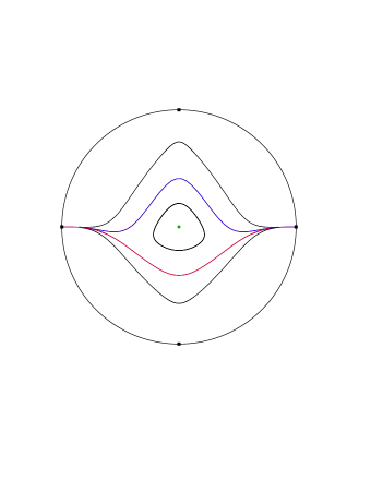
Figure 1. Phase portrait of $\nabla H_{f}^{\perp}$ in the Poincaré disc.

Example 9.

Let $f=(f_{1},f_{2}):\mathbb{R}^{2}\to\mathbb{R}^{2}$ be defined by $f_{1}(x,y)=e^{x}\cos y-1$, $f_{2}(x,y)=e^{x}\sin y$. We have $\det Df(x,y)=e^{2x}$. Moreover, the points $z_{k}=(0,2k\pi)$, $k\in\mathbb{Z}$, are the points that annihilate $f$. Therefore, the centers of $\nabla H_{f}^{\perp}$ are the points $z_{k}$, $k\in\mathbb{Z}$.

We will estimate the period annulus $\mathcal{P}_{z_{k}}$ of each center $z_{k}$.

Observe that $f(\mathbb{R}^{2})=\mathbb{R}^{2}\backslash\{(-1,0)\}$, thus the biggest ball centered at $(0,0)$ contained in $f(\mathbb{R}^{2})$ is $B_{1}$. In order that a point $(x,y)$ be such that $f(x,y)\in B_{1}$, it is necessary that $\cos y>0$, which happens in the intervals $\left((4k-1)\pi/2,(4k+1)\pi/2\right)$, $k\in\mathbb{Z}$.

It is easy to see that $f$ is injective in each of the sets $\mathbb{R}\times((4k-1)\pi/2,(4k+1)\pi/2)$, $k\in\mathbb{Z}$.

Thus the exact set $\mathcal{P}_{z_{k}}$ is from Corollary 4 the set satisfying $f_{1}(x,y)^{2}+f_{2}(x,y)^{2}<1$, with $y\in\left((4k-1)\pi/2,(4k+1)\pi/2\right)$. Straightforward calculations show that this is the set

$$\mathcal{P}_{z_{k}}=\left\{(x,y)\in\mathbb{R}^{2}\ |\ e^{x}<2\cos y,\ (4k-1)\pi<2y<(4k+1)\pi\right\}.$$

Since $2H_{f}=f_{1}^{2}+f_{2}^{2}$, it follows that the connected components of the level sets $H_{f}^{-1}\{h\}$ with $h<1/2$ give the periodic orbits of each center, and the connected components of the level set $H_{f}^{-1}\{1/2\}$ give the boundary of the period annulus of each center. Finally, it is simple to see that the level sets $H_{f}^{-1}\{h\}$ with $h>1/2$ are connected. An overview of the level sets of $H_{f}$ in the plane can be seen in Figure 2.

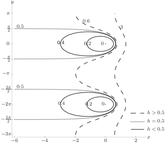
Figure 2. The level sets of $H_{f}$.

Next example presents a non-injective polynomial map in $\mathbb{R}^{2}$ producing two centers.

Example 10.

Let $g=(g_{1},g_{2}):\mathbb{R}^{2}\to\mathbb{R}^{2}$ be the Pinchuk map as defined in [3]. The image $g(\mathbb{R}^{2})$ does not contain the points $(0,0)$ and $(-1,-163/4)$. Moreover, all the points of the curve $\left(P(s),Q(s)\right)$ defined by

$$P(s)=s^{2}-1,\ \ \ \ Q(s)=-75s^{5}+\frac{345}{4}s^{4}-29s^{3}+\frac{117}{2}s^{2}-\frac{163}{4},$$

$s\in\mathbb{R}$, with the exception of $(0,0)$ and $(-1,-163/4)$, have exactly one inverse image under $g$. All the other points of $\mathbb{R}^{2}$ have two inverse images. The curve $\left(P(s),Q(s)\right)$ crosses the $y$-axis in $y=0$ and in $y=208$. For details on these results, see [3].

We consider $f:\mathbb{R}^{2}\to\mathbb{R}^{2}$ defined by translating the Pinchuk map as follows

$$f(x,y)=\big{(}g_{1}(x,y),g_{2}(x,y)-200\big{)}.$$

Let $z_{0}^{1}$ and $z_{0}^{2}$ be the two elements of the set $f^{-1}\{(0,0)\}=g^{-1}\{(0,200)\}$. From Lemma 1 the points $z_{0}^{1}$ and $z_{0}^{2}$ are centers of $\nabla H_{f}^{\perp}$.

Since $(0,-200)$ and $(-1,-163/4-200)$ are the only points not contained in $f(\mathbb{R}^{2})$, the greatest open ball centered at $(0,0)$ contained in $f(\mathbb{R}^{2})$ is $B_{200}$. Moreover, from the properties of the Pinchuk map mentioned above, there exists an entire curve with just one inverse image under $f$ in this ball. All the other points have two pre-images. We consider $B_{r}$ the greatest ball centered at $(0,0)$ such that all its points have two inverse images under $f$. The inverse image of $B_{r}$ gives two open sets. One of them, say the one containing $z_{0}^{1}$, is the entire period annulus of the center $z_{0}^{1}$. The other open set is properly contained in the period annulus of the center $z_{0}^{2}$. This period annulus is mapped bijectively onto the open ball $B_{200}$.

4. The polynomial case

In this section given a polynomial vector field $\mathcal{X}$, we denote by $p(\mathcal{X})$ the Poincaré compactification of $\mathcal{X}$. For details we refer the reader to chapter 5 of [6]. As usual we call the singular points of $p(\mathcal{X})$ located in the equator of the Poincaré sphere $\mathbb{S}^{2}$ the infinite singular points of $\mathcal{X}$. The other singular points we call finite singular points.

For a center $z_{0}$ of a polynomial vector field $\mathcal{X}$ we use the following classification of Conti, see [5]. We say that the center $z_{0}$ is of type A if $\partial\mathcal{P}_{z_{0}}=\emptyset$, i.e. the center is global, of type B if $\partial\mathcal{P}_{z_{0}}\neq\emptyset$ and $\partial\mathcal{P}_{z_{0}}$ is unbounded and does not contain finite singular points, of type C if $\partial\mathcal{P}_{z_{0}}$ contains finite singular points and is unbounded, and of type D if $\partial\mathcal{P}_{z_{0}}$ contains finite singular points and is bounded. We remark that $\partial\mathcal{P}_{z_{0}}$ can never be a periodic orbit $\gamma$ of $\mathcal{X}$, otherwise let $\pi$ be the return Poincaré map defined in a transversal section $S$ through $\gamma$. Since $\pi$ is analytic and it is the identity map in the portion of $S$ contained in $\mathcal{P}_{z_{0}}$, it follows that it must be the identity in $S$, a contradiction with the fact that $\gamma$ is the boundary of $\mathcal{P}_{z_{0}}$.

Let $q$ be an infinite singular point of the polynomial vector field $\mathcal{X}$ and $h$ be a hyperbolic sector of $q$ in the Poincaré sphere. We say that $h$ is degenerate if its two separatrices are contained in the equator of $\mathbb{S}^{2}$. Otherwise we say that $h$ is non-degenerate.

In the following we give more equivalences to the injectivity of $f$ in case the Hamiltonian $H_{f}$ is polynomial.

Theorem 11.

Let $f:\mathbb{R}^{2}\to\mathbb{R}^{2}$ be a $C^{2}$ map satisfying (3) and $z_{0}\in\mathbb{R}^{2}$ such that $f(z_{0})=(0,0)$. If $H_{f}$ is polynomial the following statements are equivalent:

• $f$ is injective and $f\left(\mathbb{R}^{2}\right)=\mathbb{R}^{2}$ or $f\left(\mathbb{R}^{2}\right)$ is an open ball centered at $(0,0)$.

• The center $z_{0}$ of $\nabla H_{f}^{\perp}$ is of type A.

• The center $z_{0}$ of $\nabla H_{f}^{\perp}$ is not of type B.

• The Hamiltonian vector field $\nabla H_{f}^{\perp}$ has no infinite singular points or each of them is formed by two degenerate hyperbolic sectors.

Proof.

Statements (a) and (b) are equivalent from Theorem 2. Moreover, since from Lemma 1 the finite singular points of $\nabla H_{f}^{\perp}$ are centers, it follows that $\partial\mathcal{P}_{z_{0}}$ does not contain finite singular points. Therefore $\nabla H_{f}^{\perp}$ can not have centers of type C or D. Hence (b) is also equivalent to (c). It is also clear that (b) implies (d).

Finally if the center $z_{0}$ is of type B, it follows that $\nabla H_{f}^{\perp}$ has at least one unbounded orbit, and thus there exist an infinite singular point without a degenerate hyperbolic sector. Hence (d) implies (c). This finishes the proof. ∎

Remark 12.

We remark that the assumption on the shape of $f\left(\mathbb{R}^{2}\right)$ in statement (a) of Theorem 11 is essential in general. Recall the above Example 8.

If $f$ is assumed to be polynomial, then we can drop this hypothesis, as polynomial injective maps are onto, from [1].

References

- [1] A. Białynicki-Birula and M. Rosenlicht, Injective morphisms of real algebraic varieties, Proc. Amer. Math. Soc. 13 (1962), 200–203.
- [2] F. Braun, J. Giné and J. Llibre, A sufficient condition in order that the real Jacobian conjecture in holds, J. Differential Equations 260 (2016), 5250–5258.
- [3] L.A. Campbell, The asymptotic variety of a Pinchuk map as a polynomial curve, Appl. Math. Lett. 24 (2011), 62–65.
- [4] A. Cima, F. Mañosas and J. Villadelprat, Isochronicity for Several Classes of Hamiltonian Systems, J. Differential Equations 157 (1999), 373–413.
- [5] R. Conti, Centers of planar polynomial systems. A review, Matematiche (Catania) 53 (1998), 207–240
- [6] F. Dumortier, J. Llibre and J.C. Artés, Qualitative theory of planar differential systems, Universitext, Springer–Verlag, 2006.
- [7] L. Gavrilov, Isochronicity of plane polynomial Hamiltonian systems, Nonlinearity 10 (1997), 433–448.
- [8] F. Mañosas and J. Villadelprat, Area-preserving normalizations for centers of planar Hamiltonian systems, J. Differential Equations 179 (2002), 625–646.
- [9] M. Sabatini, A connection between isochronous Hamiltonian centres and the Jacobian conjecture, Nonlinear Anal. 34 (1998), 829–838.
- [10] M. Sabatini, Commutativity of flows and injectivity of nonsigular mappings, Ann. Polon. Math. 76 (2001), 159–168.