Mass loss rates from mid-IR excesses in LMC and SMC O stars

Abstract

We use a combination of $BVJHK$ and Spitzer [3.6], [5.8] and [8.0] photometry to determine IR excesses for a sample of 58 LMC and 46 SMC O stars. This sample is ideal for determining IR excesses because the very small line of sight reddening minimizes uncertainties due to extinction corrections. We use the core-halo model developed by Lamers & Waters (1984a) to translate the excesses into mass loss rates and demonstrate that the results of this simple model agree with the more sophisticated CMFGEN models to within a factor of 2. Taken at face value, the derived mass loss rates are larger than those predicted by Vink et al. (2001), and the magnitude of the disagreement increases with decreasing luminosity. However, the IR excesses need not imply large mass loss rates. Instead, we argue that they probably indicate that the outer atmospheres of O stars contain complex structures and that their winds are launched with much smaller velocity gradients than normally assumed. If this is the case, it could affect the theoretical and observational interpretations of the “weak wind” problem, where classical mass loss indicators suggest that the mass loss rates of lower luminosity O stars are far less than expected.

1 Introduction

The winds of massive stars power and enrich the ISM, affect the evolution of the stars, determine their ultimate fate and the nature of their remnants, influence the appearance of the integrated spectra of young, massive clusters and star-bursts, and play a major role in the initial stages of massive star cluster formation and their subsequent evolution. Consequently, reliable measurements of mass loss rates due to stellar winds are essential for all of these subjects.

Stellar winds are driven by radiative pressure on metal lines (Castor et al. 1975, CAK). However, in recent years, it has become apparent that the winds are far more complex than the homogeneous, spherically symmetric flows envisioned by CAK. Instead, they have been shown to contain optically thick structures which may be quite small or very large. Further, these structures are thought to have non-monotonic radial velocities. Co-rotating interaction regions (CIRs) (Cranmer & Owocki, 1996, Lobel & Blomme, 2008) are examples of large structures and wind fragments caused by the line deshadowing instability (LDI) (Owocki et al. 1988, Sunqvist et al. 2011, Šurlan et al. 2012) are examples of small structures. Until the details of these flows are unraveled, we cannot reliably translate observational diagnostics into physical quantities such as mass loss rates. To progress, a firm grasp on the underlying physical mechanisms which determine the wind structures is required. The state of affairs can be seen in recent literature where the values of observationally derived mass loss rates have swung back and forth by factors of 10 or more (Puls et al. 2006, Massa et al. 2003, Fullerton et al. 2006, Sunqvist et al. 2011, Šurlan et al. 2012).

Evidence for large scale wind structure first emerged when the variability was observed in H$\alpha$ line profiles (Underhill, 1961, Rosendhal, 1973a, b and Ebbets 1982). This was followed by studies of UV P Cygni line variability by several investigators, who examined the behavior of discrete absorption components (DACs), which traverse UV wind line profiles and suggest the presence of large, coherent structures propagating through the winds (e.g., Kaper et al. 1999, Prinja et al. 2002). Similar features are observed in LMC and SMC O stars (Massa et al. 2000) and in planetary nebula central stars (Prinja et al. 2012), suggesting these structures are a universal property of radiatively driven flows.

Perhaps the most compelling evidence that the winds contain optically thick structures was provided by Prinja & Massa (2010) who used doublet ratios to demonstrate that apparently unsaturated wind lines often arise in structures that are optically very thick, but cover only a fraction of the stellar surface. Further, Massa & Prinja (2015) used UV excited state wind lines to demonstrate that at least some of these structures are quite large and originate very near or on the stellar surface. Additional evidence for large scale structure has been deduced from X-ray variability (e.g., Massa et al. 2014, Rauw et al. 2015). Models which account for optically thick structures have been developed (Sundqvist, Puls & Feldmeier 2010, and Šurlan et al. 2012), and they provide somewhat better descriptions of the observations. However, one must keep in mind that whenever optically thick structures are included in a model, geometry matters. Therefore, it is essential to constrain the shape of the structures as much as possible, and the best way to probe the geometry is to examine all of the spectral diagnostics available. Only when all of the available diagnostics have been examined, and a model constructed that can simultaneously explain them all, will we be assured that observationally determined mass loss rates are meaningful. Each diagnostic provides an important piece of the puzzle.

The IR fluxes of OB stars present an important diagnostic that has been largely neglected. It was shown early on that emission from OB star winds should be detectable at IR and radio wavelengths (Wright & Barlow 1975, Panagia & Felli 1975). This realization spawned observations of OB stars at near and mid-IR wavelengths (e.g., Castor & Simon 1983, Abbott et al. 1984), but the results were considered untrustworthy for two reasons. First, IR photometric systems were still evolving at the time and poorly calibrated. As a result, only rather large excesses could be trusted. Second, accurate reddening corrections are essential for interpreting IR excesses, since the excess must be measured relative to the stellar flux at a wavelength assumed to be free of wind emission, typically $V$ band photometry. However, there are very few lightly reddened, luminous Galactic OB stars, and the exact form of the IR reddening law was poorly characterized at the time of the early studies. Nevertheless, there remains strong motivation to study IR excesses since, as Puls et al. (2006) demonstrated, the wavelength dependence of the mid-IR SED can provide important information on the radial dependence of clumping in the wind.

This paper has two major goals. The first is to use near IR (NIR) and mid-IR observations of Magellanic cloud O stars to determine their IR excesses and compare them to theoretical expectations. The second is to compare the IR mass loss rates of LMC and SMC stars to examine how metallicity affects the results. In § 2 we describe our sample of stars. In § 3, we derive the physical parameters of the stars and quantify the influence of interstellar extinction. In § 4 we motivate, describe and justify the simplified model we use to derive mass loss rates from IR excesses. In § 5 we describe how we fit the IR photometry and present our results. In § 6, we quantify the sensitivity of the derived mass loss rates to various systematic effects. In § 7 we discuss the implications of our results.

2 The Sample and Data

With the advent of Spitzer, well calibrated mid-IR observations of the Magellanic Clouds became available, thanks to the Spitzer SAGE legacy data products provided by Meixner et al. (2006) for the LMC and Gordon et al. (2011) for the SMC. These data present the opportunity to obtain a large, uniform set of IR derived mass loss rates from lightly reddened stars, with well-determined luminosities. Bonanos et al. (2009, 2010) took advantage of the new data and compiled catalogs by starting with all massive stars in the LMC and SMC with high quality spectral classifications, and then matching them to entries in the Spitzer and other photometric data bases. The catalogs contain $U$, $B$, $V$, and $I$ from various sources and $JHK$ photometry (primarily from the Two Micron All Sky Survey, 2MASS; Skrutskie et al. 2006 and the targeted IRSF survey, (Kato et al. 2007), together with Spitzer IRAC [3.6], [4.5], [5.8] and [8.0] photometry and some MIPS [24] photometry (see Bonanos et al. for details). The Bonanos et al. catalogs contain 341 LMC and 195 SMC O stars with high quality spectral types and optical, NIR and Spitzer mid-IR photometry through [4.5]. Bonanos et al. also demonstrated that the O stars had detectable IR excesses due to winds, but did not perform a quantitative analysis of individual stars.

In this paper, we concentrate on a sub-sample of the Bonanos et al. (2009, 2010) catalogs, namely those O stars which are also in the Blair et al. (2009) FUSE sample. This will allow direct comparison of results derived from different diagnostics in many cases. We rejected stars later than B0, since their winds can contain a significant fraction of neutral hydrogen. This fraction can be strongly dependent upon NLTE processes and clumping in the wind, both of which introduce unwanted complications into the modeling (see Petrov et al. 2014). We also rejected WR stars since their massive winds require a full treatment of electron scattering, which we neglect. After imposing these restrictions, our sample contained 46 SMC and 58 LMC O stars (see Tables LABEL:tab:smcstars and LABEL:tab:lmcstars).

We supplemented the CCD based optical photometry listed by Bonanos et al. with photoelectric $V$ and $B$ photometry from the literature whenever possible and assigned errors of 0.03 mag to each. Priority was given to the photoelectric photometry. We eliminated the Spitzer MIPS data, since very few stars were detected at [24]. The $I$ band photometry was also eliminated for reasons discussed in § 4, and $U$ band photometry was not included since CCD $U$ band photometry (which is all that exists for most of the stars) often has calibration issues and it was not needed for our purposes.

The Bonanos et al. (2009) calibrations and effective wavelengths were used, with two exceptions. First, the Kato et al. (2007) IRSF to 2MASS conversion factors were applied to the IRSF photometry. Second, the $B$ band zero magnitude flux was decreased by 4% with respect to the one listed by Bonanos et al.. This was needed to produce $(B-V)$ indices which agree with the Fitzpatrick & Massa (2005) calibration and to insure that derived $E(B-V)$ values are greater than 0.

3 Stellar Parameters and Reddening

To determine the underlying photospheric flux of each program star and its expected theoretical mass loss rate, we must know its physical parameters, i.e., mass, effective temperature, luminosity and chemical composition. We obtain these from the SMC and LMC spectral type to luminosity, effective temperature and mass calibrations provided by Weidner & Vink (2010). Tables LABEL:tab:smcstars and LABEL:tab:lmcstars summarize the physical parameters for the SMC and LMC samples, respectively. We used the spectral types from the Bonanos et al. catalogs for most stars, and exceptions are noted in the tables.

Observed color excesses, $E(B-V)_{obs}$, were determined using $(B-V)_{0}$ values from TLUSTY model atmospheres (Lanz & Hubeny 2002) with the appropriate $T_{\rm eff}$, $\log g$ and metallicity. These same models were used to determine the photospheric fluxes of the stars.

To characterize the optical and IR extinction, we adopt the Weingartner & Draine (2001) curves for the SMC and LMC. As with all other wavelength ranges, the form of the IR extinction law is variable (e.g., Fitzpatrick & Massa 2009, Schlafly et al. 2016). However, because reddening is minimal in most cases, the exact form of the extinction curve used is not too important. Nevertheless, the effects of variations in $R(V)\equiv A(V)/E(B-V)$ are taken into account by allowing $E(B-V)$ to be a free parameter in fitting the IR continua (see § 5). The consequences of this action are examined in § 6.

4 The Wind Model

4.1 Formulation of the model

In general, the wind density of a smooth spherically symmetric flow from a star of radius $R_{\star}$ is determined by the wind velocity law and the mass loss rate, $\dot{M}$. Typically, the velocity law for a wind with a terminal velocity $v_{\infty}$ is assumed to have the form

$$w=\left(1-\frac{a}{x}\right)^{\beta}$$ (1)

where $w=v/v_{\infty}$, $x=r/R_{\star}$, $a=1-w_{0}^{1/\beta}$ and $w_{0}=w(x=1)$. These wind laws have a maximum velocity gradient at $x=1$, and laws with larger $\beta$ parameters accelerate more slowly. In the following, we adopt $\beta=1$ and $w_{0}=0.01$, which are typical values for OB stars. Whenever possible, $v_{\infty}$ values derived from UV observations were collected from the literature. If none were available, we derived $v_{\infty}$ from the stellar parameters and the prescription provided by Vink et al. (2001). Their method was also used to calculate theoretical mass loss rates, $\dot{M}$(Vink). The mass loss rates derived from IR excesses turn out to be more sensitive to the wind parameters than the stellar parameters.

The continuity equation relates the wind density and the velocity

$$\rho=\frac{\dot{M}}{4\pi R_{\star}^{2}v_{\infty}x^{2}w(x)}$$ (2)

Thus, $\rho$ varies rapidly as $x$ approaches 1; is proportional to $\dot{M}$; is inversely proportional to $v_{\infty}$; and, is denser at a given $x$ for larger $\beta$. The IR emission from a wind is dominated by free-free and free-bound emission and absorption by H and He. It can originate very near the star (the exact radius depends upon wavelength and wind density).

Because our goal is to survey several objects in order to determine mean properties, identify outliers, contrast differences between the LMC and SMC, compare the results with theoretical expectations, and search for trends. To accomplish this, we model the observed IR excesses of 104 O stars. Consequently, we sought the simplest available model that captures the essential physics of IR continuum formation. A computational fast model which suffers only a minimal loss of precision is the one developed by Lamers & Waters (1984a, 1984b, LWa, LWb). This is a core-halo model wherein the flux from a static plane parallel model atmosphere is embedded in a stellar wind and both the emission and absorption by the wind material are treated in detail. As is typical, the wind is assumed to be uniform and spherically symmetric with a density structure set by the velocity law. For simplicity, it is also assumed that the wind is in LTE at a fixed temperature, $T_{w}$, typically 0.8 – $0.9\times T_{eff}$.

We employ the LWa model together with TLUSTY models (with appropriate SMC or LMC metallicities) for the underlying photospheres. In this core-halo formulation, the observed flux, $f(\lambda)$, and the flux of the underlying photosphere, $f(\lambda)_{p}$, are related by

$$f(\lambda)=\left[Z(\lambda)_{1}+Z(\lambda)_{2}\frac{f(\lambda)_{w}}{f(\lambda)_{p}}\right]f(\lambda)_{p}$$ (3)

where $f(\lambda)_{w}$ is a Planck function with $T=T_{w}$, and $Z_{1}$ and $Z_{2}$ are functions which represent the attenuation of the stellar flux by the wind and the emission and self-absorption of the wind, respectively. These functions are integrals over the impact parameter, $q$, and can be calculated very quickly once the optical depth through the wind as a function of impact parameter, $\tau(q)$, is known. While determining $\tau(q)$ can be time consuming, it only has to be done once for a given set of wind law parameters, $\beta$ and $w_{0}$. Consequently, tables of $\tau(q)$ as a function of $q$ can be constructed for each velocity law and then scaled by the mass loss rate, terminal velocity and $T_{w}$. These can be integrated very quickly over $q$ to obtain a specific model.

When fitting the models to the observations, we use a version of equation (3) which is normalized to the flux at $V$ and accounts for extinction, viz,

$$\frac{f(\lambda)}{f(V)}=\frac{[Z(\lambda)_{1}+Z(\lambda)_{2}f(\lambda)_{w}/f(\lambda)_{p}]f(\lambda)_{p}10^{-0.4A(\lambda)}}{[Z(V)_{1}+Z(V)_{2}f(V)_{w}/f(V)_{p}]f(V)_{p}10^{-0.4A(V)}}$$ (4)

where $f(\lambda)_{p}$ is a TLUSTY model which depends on $T_{eff}$, $\log g$ and metallicity, and $Z_{1}(\lambda)$ and $Z_{2}(\lambda)$ depend on the velocity law parameters, $\beta$, $w_{0}$ and $v_{\infty}$ and $\dot{M}$. We also assume that $Z(V)_{1}=1$ and $Z(V)_{2}=0$, which gives

$$\frac{f(\lambda)}{f(V)}=\left[Z(\lambda)_{1}+Z(\lambda)_{2}\frac{f(\lambda)_{w}}{f(\lambda)_{p}}\right]\frac{f(\lambda)_{p}}{f(V)_{p}}10^{-0.4E(\lambda-V)}$$ (5)

In performing the fits, we adopt a logarithmic version of this equation,

$$\log\frac{f(\lambda)/f(V)}{f(\lambda)_{p}/f(V)_{p}} = \log\left[Z(\lambda)_{1}+Z(\lambda)_{2}\frac{f(\lambda)_{w}}{f(\lambda)_{p}}\right]$$ (6)

$$-0.4E(B-V)k(\lambda-V)$$

where $k(\lambda-V)\equiv E(\lambda-V)/E(B-V)$, so $E(\lambda-V)=E(B-V)k(\lambda-V)$. Note that $k(\lambda-V)<0$ for $\lambda>\lambda_{V}$.

Following LWa, we do not extend the wind model to wavelengths shorter than 1 µm. Shorter wavelengths require including the Paschen jump at 0.82 µm. This could introduce sizable uncertainties. The strength of the Paschen jump is much stronger than the Brackett jump (at 1.46 µm) because the populations of the Hydrogen levels increase dramatically with decreasing quantum number. Further, the populations of the lower hydrogen levels are strongly affected by NLTE effects, so the exact strength of the jump cannot be accurately predicted by the LTE assumption of the LWa model. As a result, we bypass the problem by not including $I$ band photometry in the fits, which is the only filter strongly affected. In addition, available $I$ band calibrations are not very reliable (see Fitzpatrick & Massa 2005).

Because the LWa core-halo models can be calculated almost instantaneously, they are ideal for the current work because we use a non-linear least squares fitting routine, where each fit typically involves several tens of model calculations, and this has to be done for 104 stars. In addition, we also examine how a variety of constraints and systematic errors affect the results, a feat which would be extremely time consuming for more sophisticated models. We also ignore the effects of electron scattering, but this should be a minor effect for the stars and wavelengths considered here.

A final simplification used to increase calculation speed was to apply a photometric calibration based on effective wavelength, $\lambda_{eff}$. We tested the validity of this approach by comparing the fluxes derived this way to those determined from integrating over filter response curves. Over the small range of intrinsic colors and color excesses in the current sample, the effects were all less than 1%.

4.2 Accuracy of the model

To determine the accuracy of the mass loss rates determined by the simple LWa model, we performed the following experiment. We employed the unclumped CMFGEN models calculated by Martins & Plez (2006) as surrogates for actual stars. These were then fit with LWa models, using eq. (6). To begin, we constructed a set of Galactic abundance TLUSTY models whose $T_{\rm eff}$ and $\log g$ values correspond to the CMFGEN models. For the LWa models, we used $\beta=0.9$ (same as the CMFGEN models used) and assumed $w_{0}=0.01$ since, unlike the CMFGEN models, the LWa models do not continue into the photosphere. We set $T_{w}=0.9T_{eff}$, since this gave the best overall agreement. The near equality of the wind and stellar temperatures is reasonable since, at the wavelengths considered here, the bulk of the wind emission comes from very near the stellar surface. The fits also allowed for reddening to be present as well, using a Weingartner & Draine (2001) $R(V)=3.1$ extinction curve. This simulates fitting actual data, since any difference between the LWa models and the CMFGEN models which has a wavelength dependence similar to an extinction curve will be absorbed into the measured extinction. We also allowed for a 2% error in each point, to simulate photometric errors.

All of the fits were excellent, with reduced $\chi^{2}<1$. A few aspects of the fits are noteworthy. First, two models ($T_{\rm eff}$= 32,500K, $\dot{M}$$\times 10^{6}=0.011$ and $T_{\rm eff}$= 37,500K, $\dot{M}$$\times 10^{6}=9.33$) do not fit the trends defined by models with similar parameters. The reason for this discord is unknown. Second, very few of the $E(B-V)$ values derived from the fits are larger than 0.01 mag, implying that the model distinguishes between reddening and wind excesses very well. Third, some CMFGEN models with very low mass loss rates have IR continua that are fainter than the corresponding TLUSTY model, resulting in small “negative excesses”, which resulted in negative $E(B-V)$ values. This effect is likely related to differences in the structure of the outer atmospheres of the CMFGEN and TLUSTY models caused by including the dynamic nature of the outer atmosphere in the CMFGEN models. While interesting, this effect is very small, with the magnitude of the negative excesses always less than 0.01 mag.

Figure 1 summarizes the comparison of the two models. It shows the mass loss rate derived from the LWa model that provides the best fit to the IR continuum of the CMFGEN model, $\dot{M}$(IR), versus the CMFGEN $\dot{M}$s. The $\dot{M}$(IR) values are nearly identical to the CMFGEN $\dot{M}$s for models with large mass loss rates. For $\dot{M}$ $\lesssim 2\times 10^{-6}$ M_⊙ yr^-1, the $\dot{M}$(IR)s overestimate the CMFGEN $\dot{M}$s by about a factor of 2. Finally, for the smallest $\dot{M}$s, the fitting cannot detect a significant excess, resulting in $\dot{M}$(IR) $\simeq 0$.

Figure 1: Mass loss rates (in M_⊙ yr^-1) determined from LWa model fits to the IR continua of the CMFGEN models of Martins & Plez (2006), $\dot{M}({\rm IR})$, versus the CMFGEN model mass loss rates, $\dot{M}$. The points shown as squares are for CMFGEN models whose fluxes deviate from the trends of models with similar physical parameters. The upper limits are for models where the fit could not determine a significant $\dot{M}$, when photometric errors of 0.02 mag are assigned to each photometry point. The solid line is $\dot{M}$$=$$\dot{M}({\rm IR})$, and the dashed line is $\dot{M}$$=$2 $\dot{M}({\rm IR})$. Overall, the mass loss rates determined by the simple LWa models recover the CMFGEN rates very well for high mass loss rates, but then begin to overestimate the mass loss rates for models with smaller $\dot{M}$. Even so, the disagreement is typically within a factor of 2 for cases where mass loss rates are detectable.

The significant result of this exercise is that if we assume that the CMFGEN models provide a good representation of the IR continua of real stars, then the simple LWa core halo model faithfully represents actual IR continua. Further, fitting IR continua with the LWa model results in $\dot{M}$(IR)s that are very accurate for stars with $\dot{M}$ $\gtrsim 2\times 10^{-6}$ M_⊙ yr^-1, but may overestimate the actual $\dot{M}$s by a factor of 2 for $\dot{M}$ $\lesssim 2\times 10^{-6}$ M_⊙ yr^-1.

5 Results

To summarize, the following ingredients are used in the fits: Weidner & Vink (2010) tables to translate spectral types into physical parameters; TLUSTY models with these parameters to give the photospheric fluxes; and, Weingartner & Draine (2001) extinction curves to characterize the extinction. We examine the implications of these assumptions in § 6.

Figure 2: Each plot shows a model fit to the log of the fluxes minus the log of the appropriate TLUSTY model, both normalized to $V$. For each star, the observed data are shown as points, with every other curve shown as open or filled points to avoid confusion when points of adjoining SEDs overlap. The black curve is the model fit, the dotted curve dotted curve shows the reddening determined by the fit, and the dashed curve is the reddening plus the excess expected from the Vink et al. (2001) mass loss rate, $\dot{M}({\rm Vink})$. One $\sigma$ errors (often smaller than the points) are shown and successive curves are offset by 0.5 dex from the bottom for display.

Figure 3: Same as Figure 2.

Figure 4: Same as Figure 2 for the LMC sample.

For each star, the observed and TLUSTY SEDs were normalized by their $V$ band fluxes. The difference, $\log f(\lambda)/f(V)-\log f(\lambda)_{p}/f(V)_{p}$, is the IR excess. This excess was fit using equation ( 6) and a non-linear least squares routine to determine 2 free parameters: $\dot{M}$(IR), which is the mass loss rate of the best fitting LWa model and $E(B-V)$ (or, equivalently, $R(V)$, see § 6).

Figures 2 – 3 show the SMC fits, Figures 4 – 6 show the LMC fits, and Tables LABEL:tab:smcwinds and LABEL:tab:lmcwinds list the results. Because these figures show the differences between the log of the observed fluxes and the appropriate TLUSTY model, any shape is due to either reddening or wind excess. The photometry is shown as filled of open points and the best fit model for each star is shown as a thick black curve. The excess that would result from the derived reddening and the excess expected from the mass loss rate predicted using the Vink et al. (2001) formulae, $\dot{M}({\rm Vink})$, is shown as the dashed curve. The contribution of reddening to the fits is shown as a dotted curve (not always visible because it often coincides with the dashed curve). For each star, the difference between the dotted curve and the black curve is the IR excess, and the difference between the dashed curve and the black curve is the excess over the IR continuum expected for $\dot{M}({\rm Vink})$. A few stars, such as AzV 47, show little evidence of either wind excess or reddening. Several, such as AzV 120 and AzV 216, are well fit by reddening alone. For most stars, there is a clear excess relative to pure extinction and to the $\dot{M}({\rm Vink})$ curves.

In general, the fits in Figures 2 – 6 are quite good. However, four stars: Az V207, AzV 461, NGC346-026 and AzV 235, have extremely large excesses and are poorly fit. The $\dot{M}$(IR) for these stars are unreliable since their huge excesses suggest circumstellar disks (see Figure 10 in Bonanos et al. 2010). Consequently, stars with $\dot{M}({\rm IR})$/$\dot{M}({\rm Vink})$$>100$ (more than twice the next largest ratio) are identified as probable disks systems in Table LABEL:tab:smcwinds (all are in the SMC). Notice too, that there is evidence that the IR fluxes varied for some stars with large excesses. For example, the two sets of nearly parallel, but off set, points for AzV 243 are from the two $JHK$ surveys, which were obtained at different epochs.

Figure 5: Same as Figure 4.

Figure 6: Same as Figure 4.

A few other properties of the SEDs are also noteworthy. For example, the SEDs of a few stars, such as AzV435 and Sk$-71^{\circ}46$, show the effects of relatively large reddening. It is also interesting to contrast the excesses and $\dot{M}$(IR)s of the O2 star Sk$-70^{\circ}90$ and the O4.5 star Sk$-67^{\circ}108$. The former has a smaller excess, but a larger $\dot{M}$(IR). This is because the O2 star has a much larger $v_{\infty}$, so the wind density (and IR emission) is lower for the same $\dot{M}$(IR).

While the fits for most stars shown in Figures 2 – 6 appear to have distinct IR excesses, the evidence is marginal in some cases (e.g., AzV69, AzV135, BI 208 and Sk$-67^{\circ}$118). This is an important point since even a small IR excess can imply a fairly large $\dot{M}$(IR), $\sim 10^{-6}$ $M_{\odot}$ yr^-1, which can be far larger than expected. To address this problem, all of the stars were fitted a second time, with $E(B-V)$ as the only free parameter and $\dot{M}$(IR) set to 0. We then formed the ratio of the $\chi^{2}$s for the fits with and without mass loss and compared them to an $F$-distribution. Stars whose ratios correspond to a 50% or more probability of being drawn from the same distribution are flagged in Tables LABEL:tab:smcwinds and LABEL:tab:lmcwinds, since there is a good chance that they have no detectable mass loss.

Tables LABEL:tab:smcwinds and LABEL:tab:lmcwinds contain several stars whose fits result in relatively large $\chi^{2}$. Ignoring the probable disks, an inspection of Figures 2 – 6 reveals that nearly all of the fits with $\chi^{2}\geq 4$ are due to a large discrepancy in the two sets of $JHK$ photometry. This means that either the photometry errors are incorrect, or that the $JHK$ fluxes are variable. Whatever the case, the fits tend to go through the mean of the two sets and usually fit the mid-IR quite well. Since it is the Spitzer fluxes which determine $\dot{M}$(IR), we believe that most of these fits are better than their $\chi^{2}$ would indicate. However, there are two cases that cannot be explained as a discordant NIR photometry. One is AzV 388, whose continuum seems to have a distinctly different shape than expected, for reasons that are not clear. The other is AzV 435 whose derived $E(B-V)$ is the largest of the entire sample. Further, it has largest difference between $E(B-V)$ and $E(B-V)_{obs}$, suggesting a peculiar extinction curve, whose shape may be very different from the one used in the fitting, resulting in a poor fit. This case illustrates the difficulties encountered when fitting the IR continua of heavily reddened stars.

Figure 7 shows the ratio of the derived $\dot{M}$(IR) divided by $\dot{M}({\rm Vink})$ for all of the program stars plotted against $\dot{M}({\rm Vink})$. The red symbols are for LMC stars and the black symbols for SMC stars. The downward pointing arrows indicate stars whose best fits implied $\dot{M}({\rm IR})$ $=0$, stars with a 50% or more probability of having no wind are shown as open symbols, and stars whose fits had a $\chi^{2}\geq 4$ are shown as crosses. Two aspects of Figure 7 are worth noting. The first is that for $\dot{M}({\rm Vink})$ $\gtrsim 10^{-6}\;M_{\odot}$ yr^-1, the relation between the observed and expected mass loss rates tightens, and $\dot{M}({\rm IR})$ $\simeq 2$ $\dot{M}({\rm Vink})$. The second is that for $\dot{M}({\rm Vink})$ $\lesssim 10^{-7}\;M_{\odot}$ yr^-1, even when the non-detections, probable non-detections and stars with obvious disks are ignored, more than half of the stars still have solid detections, implying that the large measured excesses are quite real.

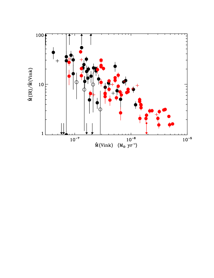
Figure 7: Ratios of the mass loss rates determined from IR excesses, $\dot{M}$(IR), to the theoretical mass loss rates, $\dot{M}({\rm Vink})$, versus $\dot{M}({\rm Vink})$. Red and black points are for the LMC and SMC samples, respectively. Open circles represent stars whose measured $\dot{M}$(IR)s are consistent with zero, downward arrows are for stars whose best fits give $\dot{M}$(IR$)=0$, crosses are for stars with reduced $\chi^{2}>4$ and upward arrows are for stars with very large mass loss rates, probably from disks.

6 Systematic effects

This section examines how the derived mass loss rates are affected by errors in: spectral classifications; the neglect of wind emission on the $B$ and $V$ photometry; variations in the extinction curves; the assumed wind temperature; and, the velocity law parameters.

Changing the spectral and luminosity classes (and, hence, the stellar parameters) changes $f(\lambda)_{p}$ and $\dot{M}({\rm Vink})$. Nevertheless, simulations showed that the derived $\dot{M}({\rm IR})$ were not very sensitive to classification errors of $\pm 1$ spectral or luminosity class and changed by less than 20% in both cases.

Comparisons to CMFGEN models (§ 4), suggest that our assumption that $B$ and $V$ are unaffected by wind emission is reasonable in most cases. However, in the few instances where the wind emission is strong enough to affect the optical photometry, it will contaminate $V$ more than $B$. This creates an intrinsic $E(B-V)$, causing an over correction for extinction which, in turn, leaves less excess to be accounted for by $\dot{M}$(IR), resulting in an underestimate of $\dot{M}$(IR). Since our major concern is effects that might lead us to over estimate $\dot{M}$(IR), this issue is not considered further.

Variations in the extinction law are another concern. Figure 8 demonstrates how changing $E(B-V)$ or $R(V)$ are equivalent over the wavelength range of interest. It shows two Weingartner & Draine (2001) Galactic curves: one for $R(V)=3.1$ and one for $R(V)=5.5$ divided by 1.7. The locations of the photometric bands are also indicated. The figure shows that for wavelengths longer than $V$, rescaling an extinction curve with one value of $R(V)$ results in a good approximation of an extinction curve with a different $R(V)$. However, for large values of $E(B-V)$, the differences can become important, introducing errors of 0.1 mag or more. That is why it is best to derive IR excesses for stars with small color excesses.

Figure 8: Comparison of Weingartner & Draine (2001) extinction curves for $R(V)=3.1$ (black curve) and $R(V)=5.5$ (dashed curve). The $R(V)=5.5$ has been divided by 1.7 to demonstrate how very different curves can appear proportional for wavelengths longer than $V$.

The degeneracy of $E(B-V)$ and $R(V)$ was the motivation for allowing $E(B-V)$ to be a free parameter when fitting the SEDs instead of simply setting it equal to $E(B-V)_{obs}$. This accommodates possible variations in $R(V)$. If the actual value of $R(V)$ along the line of sight, $R(V)$₀, differs from the assumed Weingartner & Draine (2001) value, $R(V)$_WD, then it should be possible to recover $R(V)$₀, from the relation

$$E(B-V)_{obs}R(V)_{WD}=E(B-V)_{fit}R(V)_{0}$$ (7)

where $E(B-V)_{fit}$ is the excess obtained from the fit. Figure 9 shows $R(V)$₀ plotted against $E(B-V)$_obs for the SMC sample. Considering that all of the excesses are small and that the errors are large, we see that there is a general trend for $R(V)$₀ to decrease with increasing $E(B-V)_{obs}$. This is consistent with the sight lines passing through a small amount of foreground, Galactic dust, with an $R(V)$$\sim 4$ and then passing through more and more SMC dust with $R(V)\sim 2.5$. Although the line of sight to the SMC was not included in Schlafly et al. (2017), they do detect $R(V)\sim 4$ for high latitude Galactic dust in nearby fields. Further, $R(V)=2.5$ is consistent with the SMC $R(V)$ determined by Gordon & Clayton (1998). Keeping in mind that neither the foreground nor the SMC dust are probably perfectly uniform, the general trend appears to verify our assumption that the value of $R(V)$ is changing from one line of sight to the next, and the amount of change depends on the relative amounts of Galactic and SMC dust encountered.

Figure 9: Values of $R(V)$ derived from the fits plotted against $E(B-V)$_obs for the SMC sample. Solid points have a reduced $\chi^{2}<4$ and crosses have $\chi^{2}\geq 4$. The plot suggests a foreground contribution to the extinction of $E(B-V)$$\simeq 0.05$ mag from dust with a rather large $R(V)$, which then melds into SMC dust with a much smaller $R(V)$. Both components may be rather patchy, accounting for the large scatter.

Assigning an incorrect temperature to the wind can affect the results. The wind temperature could be much higher than 0.9$T_{\rm eff}$ if shocks and their associated X-rays heat the wind to temperatures $\sim 10^{6}$K as suggested by Cassinelli et al. (2001). However, increasing $T_{w}$ to $10^{6}$ K only reduces $\dot{M}$(IR) by 30%.

Finally, we examined how changing the parameters in the velocity law, eq. (1), affects the derived mass loss rates. Changing $w_{0}$ over the range $0.005\leq w_{0}\leq 0.02$ (the most commonly used values) changed the derived $\dot{M}({\rm IR})$s by 20% or less, which is small compared to the observed disagreement between theory and observation.

It is particularly important to examine the effect of changing $v_{\infty}$ for the less luminous stars. For most of these stars, observed values are not available so we rely on the values predicted by Vink et al. (2001). When observed values are available, they are often much less than the predicted ones, but this could be a systematic effect. It is difficult to measure $v_{\infty}$ in less luminous stars, since their wind lines are typically asymmetric, lacking a distinctive blue edge. This makes the full extent of the wind absorption hard to measure and easy to underestimate. However, experiments show that reducing $v_{\infty}$ by a factor of 2 reduces $\dot{M}({\rm IR})$ by 40%. While substantial, this is too little to explain the observed $\dot{M}({\rm IR})$/ $\dot{M}({\rm Vink})$ ratios.

In contrast to the other parameters, $\beta$ can have a major effect on the derived $\dot{M}$(IR)s (as noted by LWa). Changing $\beta$ from 1 to 2.5 reduces the inferred $\dot{M}$ by a factor of 2.7. Figure 10 demonstrates this effect. It arises because a larger $\beta$ reduces the velocity gradient (increasing the density) near the surface of the star, where most of the emission occurs. We return to this issue in the next section.

Figure 10: The effect of changing $\beta$ on the derived mass loss rates for the sample shown in Figure 7. The plot shows $\dot{M}({\rm IR})$/$\dot{M}({\rm Vink})$ as a function of $\dot{M}({\rm Vink})$. Open points are $\dot{M}({\rm IR})$ derived using $\beta=1$, filled points are $\dot{M}({\rm IR})$ derived using $\beta=2.5$, and lines connect points for the same star.

7 Discussion

Our results can be summarized as follows: mass loss rates determined from IR excesses are larger than expected, increasing from about a factor of 2 for the most luminous stars to about 40 for the least luminous stars with detectable IR excesses; and, the LMC and the SMC results are similar. Because we have shown that $\dot{M}({\rm IR})$ derived by the LWa models can overestimate the actual $\dot{M}$ by a factor of 2 for stars with $\dot{M}\lesssim 2\times 10^{-6}$ M_⊙ yr^-1, these results are consistent with $\dot{M}({\rm Vink})$ $\lesssim$ $\dot{M}({\rm IR})$$\lesssim$ 2$\dot{M}({\rm Vink})$ for $\dot{M}({\rm Vink})$ $\gtrsim 2\times 10^{-6}$ M_⊙ yr^-1, growing to 5 $\dot{M}({\rm Vink})$ $\lesssim$ $\dot{M}({\rm IR})$ $\lesssim 20$ $\dot{M}({\rm Vink})$ for the least luminous stars. Thus, if we interpret the IR excesses in terms of mass loss, they infer rates that are equal to or much larger than theoretical predictions. This is in stark contrast to recent mass loss rates determined from UV wind lines, H$\alpha$ and X-ray diagnostics, which suggest rates smaller than the Vink et al. (2001) predictions by a factor of 2 to 3 (see Martins & Palacios 2017 for a summary).

However, it is well known that increasing the mass loss rate is not the only way to increase the IR emission. In this section, we argue that the large IR excesses and their implied large $\dot{M}$(IR)s are not the result of large mass loss rates. Instead, we attribute them to density and velocity structures near the base of the wind. We also consider the implications of the scatter in Figure 7 and the fact that points from stars in both galaxies are interspersed.

Throughout the discussion, we emphasize that the IR excesses in our sample originate very near the stellar surface. To see this, consider the effective radii of the IR excesses. Using a $\beta=1$ velocity law and our longest wavelength, 8.0$\mu$m, even the strongest winds in our sample (aside from the obvious disks) result in a value of the LWa parameter $E_{\nu}$ (their eq. 6) that is less than 0.01. This implies an effective radius which is only a few percent larger than the stellar radius (see LWa Figure 4).

At O star temperatures, the intensity of the IR wind emission is proportional to the density squared, and there are two ways to enhance this for a fixed mass loss rate. One is to collect most of the wind mass into structures or clumps with enhanced densities. The other is to reduce the velocity gradient, which then increases the density through the continuity equation. Since, as outlined in § 1, evidence for structure in O star winds abounds, including indications that this structure originates near the stellar surface, we suspect that this structure accounts for much of the large excesses. The notion that we are seeing effects that originate near the stellar surface is reinforced by the fact that the largest discrepancies occur for stars with lower expected mass loss rates, where we expect to see nearly to the stellar surface.

It is possible to make our results a bit more quantitative. First, consider the case where all of the excess is due to density inhomogeneities. Abbott et al. (1981) developed a simple model for how clumping enhances the observed emission. It assumes the wind consists of two components whose density ratio is $x$, where $0\leq x\leq 1$, and the fraction of the wind volume occupied by the higher density is $f_{V}$. The geometry of the structures is unspecified. Setting $x=0$ gives the largest enhancements for fixed $f_{V}$, with the ratio of the observed to actual mass loss rates being simply $f_{V}^{-1/2}$. In our case, this ratio is $\dot{M}({\rm IR})$/$\dot{M}({\rm Vink})$. For stars with smaller $\dot{M}({\rm Vink})$, this ratio varies between 5 and 20 (where an overestimate of 2 by $\dot{M}({\rm IR})$ is assumed). Thus, if the entire discrepancy is attributed to clumping, stars with weak winds must have all of the wind material confined to between 0.3 and 4% of the wind volume. This is in contrast to stars with more massive the winds, where Massa & Prinja (2015) showed that the wind structures near the photosphere are quite large and to recent H$\alpha$ results, described below.

Next, consider the effects of the velocity gradient. Figure 10 shows that increasing $\beta$ from 1 to 2.5 (which corresponds to reducing the velocity gradient at $x=1$ by a factor of 7.5 for $w_{0}=0.01$), decreases the inferred $\dot{M}({\rm IR})$ by a factor of 2.7. Thus, a large reduction in the velocity gradient can also strongly influence the mass loss inferred from the IR flux.

It is interesting to compare our results with the recent H$\alpha$ mass loss rates determined by Ramírez-Agudelo et al. (2017). For stars more luminous than $\log L/L_{\odot}\gtrsim 5.6$, (which corresponds roughly to $\dot{M}({\rm Vink})$$\gtrsim 10^{-6}$ M_⊙ yr^-1) both approaches require similar volume filling factors to bring the observational mass loss rates into accord with the theoretical ones. However, at lower luminosity, the IR mass loss rates are much larger than those determined from H$\alpha$. This can arise if the velocity gradient is small, so that the opacity at continuum wavelengths is much less than in a line like H$\alpha$. In this case, the IR emission probes more deeply into the wind and, as we saw above, a slow acceleration can greatly enhance the IR emission. Therefore, to avoid extremely large values of $f_{V}$, it seems that some combination of strong density clumping and a small acceleration at the base of the wind are required to produce the observed IR excesses. Given that the IR emission in stars expected to have low mass loss rates originates in the poorly understood transition region between the photosphere and wind, our results should not be too surprising. Instead, we should view the IR as providing important constraints on the structure of the photosphere – wind interface.

A few other aspects of Figure 7 are also of interest. First, the large intrinsic scatter in $\dot{M}({\rm IR})$ for stars with smaller $\dot{M}({\rm Vink})$ suggests that either the IR excesses are affected by physical parameters beyond those used to determine $\dot{M}({\rm Vink})$ (e.g., rotation, magnetic fields, interacting binary winds or incipient disks), or that the excesses in these stars are variable. Second, points from both the SMC and LMC overlap, implying that the physical origin of the process causing the additional excesses is independent of metallicity, and consistent with the Vink et al. (2001) treatment of different metallicities.

Our results could also have bearing on the “weak wind problem” (Martins et al. 2005). If the excesses for low luminosity stars are due to extremely compact structures and small velocity gradients near the stellar surfaces, then many of the diagnostics used to interpret weak winds could be strongly affected.

Table 1: SMC Stellar Properties

Name	Sp Ty	ref	$V$	$(B-V)$	$T_{\rm eff}$	$\log L/L_{\odot}$	$M/M_{\odot}$	$R/R_{\odot}$
AzV14	O3-4 V	B10	13.77	-0.19	44338	5.44	44.35	8.91
AzV435	O4 V	B10	14.13	-0.07	43292	5.40	41.15	8.88
AzV177	O4 V	B10	14.53	-0.21	43292	5.40	41.15	8.88
NGC346-007	O4 V((f+))	B10	14.02	-0.24	43292	5.40	41.15	8.88
AzV75	O5 I(f+)	B10	12.79	-0.16	38715	5.81	54.79	17.76
AzV61	O5 III((f))	B10	13.54	-0.18	38881	5.68	42.91	15.20
AzV377	O5 Vf	B10	14.59	-0.25	41200	5.31	35.38	8.86
AzV388	O5.5 V((f))	B10	14.12	-0.21	40154	5.27	32.78	8.87
AzV243	O6 V	B10	13.87	-0.22	39108	5.22	30.33	8.89
AzV446	O6 V	B10	14.59	-0.24	39108	5.22	30.33	8.89
AzV220	O6.5 ?fp	B10	14.50	-0.22	35929	5.67	46.83	17.64
AzV15	O6.5 I(f)	B10	13.17	-0.21	35929	5.67	46.83	17.64
AzV476	O6.5 V	B10	13.52	-0.09	38062	5.18	28.01	8.92
AzV83	O7 Iaf	B10	13.58	-0.13	35001	5.62	44.90	17.64
AzV232	O7 Iaf	B10	12.36	-0.20	35001	5.62	44.90	17.64
AzV469	O7 Ib	B10	13.20	-0.22	35001	5.62	44.90	17.64
AzV26	O7 II	B10	12.55	-0.20	35226	5.54	39.36	15.86
AzV80	O7 III	M95	13.32	-0.13	35451	5.46	33.83	14.27
AzV207	O7 V	B10	14.37	-0.22	37016	5.13	25.80	8.97
AzV208	O7 V	B10	14.15	-0.10	37016	5.13	25.80	8.97
AzV440	O7 V	B10	14.64	-0.20	37016	5.13	25.80	8.97
AzV69	OC7.5 III((f))	B10	13.35	-0.22	34593	5.41	32.05	14.08
AzV491	O7.5 III:	M95	14.72	-0.20	34593	5.41	32.05	14.08
AzV47	O8 III((f))	B10	13.38	-0.26	33736	5.35	30.39	13.92
AzV95	O8 III	B10	13.83	-0.19	33736	5.35	30.39	13.92
AzV135	O8 III	B10	13.96	-0.23	33736	5.35	30.39	13.92
AzV461	O8 V	B10	14.61	-0.21	34924	5.05	21.63	9.10
AzV261	O8.5 I	P09	13.88	-0.07	32215	5.49	40.52	17.81
AzV73	O8.5 V	M95	14.08	-0.17	33878	5.00	19.63	9.20
AzV70	O9 Ia	P09	12.38	-0.17	31287	5.44	39.35	17.93
AzV479	O9 Ib	B10	12.48	-0.15	31287	5.44	39.35	17.93
AzV378	O9 III	B10	13.88	-0.24	32021	5.25	27.29	13.65
AzV451	O9 V	M02	14.15	-0.23	32832	4.96	17.64	9.31
AzV372	O9.5 Iabw	P09	12.63	-0.18	30358	5.40	38.22	18.07
AzV456	O9.5 Ib	B10	12.89	0.09	30358	5.40	38.22	18.07
AzV238	O9.5 II	P09	13.77	-0.22	30761	5.30	31.99	15.64
AzV423	O9.5 II(n)	P09	13.28	-0.19	30761	5.30	31.99	15.64
AzV120	O9.5 III	B10	14.56	-0.23	31163	5.19	25.76	13.55
AzV170	O9.5 III	B10	14.09	-0.23	31163	5.19	25.76	13.55
AzV334	O9.5 III	B10	13.81	-0.21	31163	5.19	25.76	13.55
AzV327	O9.7 I	B10	13.25	-0.22	29987	5.38	37.78	18.14
AzV215	B0 Ia	P09	12.69	-0.09	29430	5.35	37.10	18.25
AzV235	B0 Iaw	P09	12.20	-0.18	29430	5.35	37.10	18.25
AzV104	B0 Ib	P09	13.17	-0.16	29430	5.35	37.10	18.25
AzV216	B0 IIW	M02	14.32	-0.17	29868	5.25	30.65	15.67
NGC346-026	B0 IV	E09	14.87	-0.14	30740	4.87	13.65	9.59
Notes: B10: Bonanos et al. 2010; P09: Penny & Gies (2009); M95: Massey et al. (1995);
M02: Massey et al. (2002)

Table 2: LMC Stellar Properties

Name	Sp Ty	ref	$V$	$(B-V)$	$T_{\rm eff}$	$\log L/L_{\odot}$	$M/M_{\odot}$	$R/R_{\odot}$
Sk -66 172	O2 III(f*)+OB	B09	13.13	-0.12	48849	5.93	84.09	12.92
Sk -68 137	O2 III(f*)	B09	13.35	-0.08	48849	5.93	84.09	12.92
LH64-16	ON2 III(f*)	B09	13.67	-0.22	48849	5.93	84.09	12.92
Sk -70 91	O2 III	B09	12.78	-0.23	48849	5.93	84.09	12.92
BI 237	O2 V((f*))	B09	13.98	-0.12	51269	5.82	79.66	10.24
Sk -67 166	O4 If+	B09	12.27	-0.22	41809	5.92	60.68	17.39
Sk -71 46	O4 If	B09	13.25	-0.09	41809	5.92	60.68	17.39
Sk -67 167	O4 Inf+	B09	12.54	-0.19	41809	5.92	60.68	17.39
Sk -65 47	O4 If	B09	12.51	-0.18	41809	5.92	60.68	17.39
Sk -67 69	O4 III(f)	B09	13.09	-0.16	43985	5.70	54.76	12.13
Sk -67 105	O4 f	B09	12.42	-0.15	43985	5.70	54.76	12.13
Sk -67 108	O4-5 III	B09	12.56	-0.20	43985	5.70	54.76	12.13
Sk -71 45	O4-5 III(f)	B09	11.47	-0.11	43985	5.70	54.76	12.13
Sk -70 60	O4-5 V((f))pec	B09	13.85	-0.19	46395	5.56	52.67	9.30
Sk -70 69	O5.5 V((f))	B09	13.94	-0.27	43958	5.43	43.40	8.93
Sk -67 111	O6 Ia(n)fp	B09	12.57	-0.20	37415	5.75	46.07	17.78
Sk -65 22	O6 Iaf+	B09	12.07	-0.19	37415	5.75	46.07	17.78
Sk -69 104	O6 Ib(f)	B09	12.10	-0.21	37415	5.75	46.07	17.78
Sk -66 100	O6 II(f)	B09	13.26	-0.21	38268	5.60	42.32	14.39
BI 208	O6 V((f))	B09	13.96	-0.24	41521	5.30	36.13	8.63
Sk -71 19	O6 III	B09	14.27	-0.20	39121	5.46	38.57	11.67
Sk -66 18	O6 V((f))	B09	13.50	-0.20	41521	5.30	36.13	8.63
Sk -71 50	O6.5 III	B09	13.45	-0.30	39121	5.46	38.57	11.67
Sk -70 115	O6.5 III	B09	12.24	-0.10	39121	5.46	38.57	11.67
BI 13	O6.5 V	B09	13.85	-0.19	41521	5.30	36.13	8.63
Sk -69 50	O7 If	B09	13.26	-0.13	35218	5.66	41.41	18.15
Sk -67 176	O7 Ib(f)	B09	11.82	-0.16	35218	5.66	41.41	18.15
BI 272	O7 II	B09	13.28	-0.22	35953	5.50	37.41	14.49
Sk -67 119	O7 III(f)	B09	13.33	-0.21	36689	5.34	33.41	11.58
BI 229	O7 III	B09	12.95	-0.17	36689	5.34	33.41	11.58
Sk -68 16	O7 III	B09	12.96	-0.15	36689	5.34	33.41	11.58
Sk -67 118	O7 V	B09	12.99	-0.20	39084	5.17	30.24	8.40
Sk -67 250	O7.5 II(f)	B09	12.68	-0.17	35953	5.50	37.41	14.49
Sk -67 168	O8 Iaf	B09	12.08	-0.17	33021	5.57	37.71	18.68
Sk -67 101	O8 II((f))	B09	12.63	-0.17	33639	5.40	33.44	14.70
Sk -67 191	O8 V	B09	13.46	-0.21	36647	5.04	25.12	8.24
Sk -67 174	O8 V	B09	11.67	-0.18	36647	5.04	25.12	8.24
Sk -71 41	O8.5 I	B09	12.84	-0.07	33021	5.57	37.71	18.68
BI 173	O8.5 II(f)	B09	13.00	-0.14	33639	5.40	33.44	14.70
Sk -67 38	O8.5 V	P09	13.72	-0.23	36647	5.04	25.12	8.24
BI 130	O8.5 V((f))	B09	12.55	-0.22	36647	5.04	25.12	8.24
Sk -66 171	O9 Ia	B09	12.19	-0.15	30824	5.49	34.39	19.39
Sk -69 257	O9 II	B09	12.49	-0.08	31324	5.29	29.71	15.07
Sk -70 97	O9 III	B09	13.33	-0.23	31825	5.10	25.03	11.71
Sk -70 13	O9 V	B09	12.35	-0.15	34210	4.91	20.15	8.15
Sk -65 44	O9 V	B09	13.65	-0.21	34210	4.91	20.15	8.15
BI 128	O9 V	B09	13.82	-0.25	34210	4.91	20.15	8.15
BI 170	O9.5 I	B09	13.09	-0.17	30824	5.49	34.39	19.39
Sk -68 135	ON9.7 Ia+	B09	11.36	0.00	30824	5.49	34.39	19.39
Sk -65 63	O9.7 I	B09	12.56	-0.16	30824	5.49	34.39	19.39
Sk -66 169	O9.7 Ia+	B09	11.56	-0.13	30824	5.49	34.39	19.39
Sk -65 21	O9.7 Iab	B09	12.02	-0.16	30824	5.49	34.39	19.39
Sk -69 124	O9.7 I	B09	12.81	-0.18	30824	5.49	34.39	19.39
Sk -70 85	B0 I	B09	12.30	-0.10	28627	5.40	30.85	20.34
Sk -69 59	B0 Ia	P09	12.13	-0.12	28627	5.40	30.85	20.34
Sk -68 52	B0 Ia	B09	11.54	-0.07	28627	5.40	30.85	20.34
Sk -67 76	B0 Ia	P09	12.42	-0.13	28627	5.40	30.85	20.34
Sk -66 185	B0 Iab	B09	13.11	-0.19	28627	5.40	30.85	20.34
Notes: B09: Bonanos eet al. (2009); P09: Penny & Gies (2009)

Table 3: SMC Wind Properties

Name	$v_{\infty}$	ref	$\dot{M}$(Vink)	$\dot{M}$(IR)	$E(B-V)$	$E(B-V)_{obs}$	$\chi^{2}$
	km s-1		$10^{-6}M_{\odot}$ yr-1		mag
AzV14	2000	M04	0.40	4.22 $\pm$ 0.75	0.12 $\pm$ 0.013	0.16	1.84
AzV435	1500	M07	0.48	3.20 $\pm$ 0.50	0.55 $\pm$ 0.013	0.27	6.09
AzV177	2650	M05	0.24	4.39 $\pm$ 0.88	0.04 $\pm$ 0.009	0.13	3.49
NGC346-007	2300	M07	0.28	0.91 $\pm$ 1.21	0.12 $\pm$ 0.006	0.10	1.53	*
AzV75	2100	M07	1.10	8.73 $\pm$ 1.25	0.15 $\pm$ 0.008	0.16	0.96
AzV61	2025	M09	0.80	9.53 $\pm$ 1.89	0.08 $\pm$ 0.014	0.14	0.96
AzV377	2350	M04	0.19	2.82 $\pm$ 0.74	0.06 $\pm$ 0.010	0.09	0.87
AzV388	1935	M07	0.21	0.00 $\pm$ 47.27	0.12 $\pm$ 0.005	0.12	10.04
AzV243	2125	M07	0.15	1.72 $\pm$ 0.45	0.10 $\pm$ 0.005	0.11	1.18
AzV446	1400	M05	0.25	1.08 $\pm$ 0.27	0.03 $\pm$ 0.000	0.09	0.44
AzV220	2267	VVV	0.52	11.83 $\pm$ 2.58	0.07 $\pm$ 0.015	0.09	0.35
AzV15	2125	M07	0.57	4.21 $\pm$ 0.74	0.18 $\pm$ 0.004	0.10	0.41
AzV476	2646	VVV	0.09	2.86 $\pm$ 0.71	0.25 $\pm$ 0.007	0.24	1.28
AzV83	940	M07	1.21	4.74 $\pm$ 0.78	0.16 $\pm$ 0.011	0.18	0.90
AzV232	1400	M09	0.74	8.22 $\pm$ 0.71	0.16 $\pm$ 0.007	0.11	2.39
AzV469	1550	M07	0.65	3.30 $\pm$ 1.20	0.15 $\pm$ 0.008	0.09	0.15
AzV26	2150	M07	0.35	3.04 $\pm$ 0.66	0.19 $\pm$ 0.004	0.11	1.70
AzV80	1550	E04	0.42	4.17 $\pm$ 0.57	0.10 $\pm$ 0.007	0.18	12.63
AzV207	2000	M05	0.11	1.19 $\pm$ 0.64	0.13 $\pm$ 0.005	0.10	0.90	*
AzV208	2537	VVV	0.08	57.90 $\pm$ 0.48	0.03 $\pm$ 0.000	0.22	9.72	D
AzV440	1300	M05	0.18	0.90 $\pm$ 0.42	0.12 $\pm$ 0.008	0.12	0.40
AzV69	1800	M07	0.27	3.38 $\pm$ 0.76	0.14 $\pm$ 0.007	0.09	2.40
AzV491	2167	VVV	0.21	2.09 $\pm$ 1.50	0.08 $\pm$ 0.008	0.11	0.82	*
AzV47	2140	VVV	0.16	0.00 $\pm$ 0.00	0.03 $\pm$ 0.000	0.04	18.12
AzV95	1700	M07	0.22	4.55 $\pm$ 0.99	0.16 $\pm$ 0.012	0.11	0.52
AzV135	2140	VVV	0.16	2.91 $\pm$ 0.92	0.06 $\pm$ 0.005	0.07	0.45
AzV461	2310	VVV	0.06	0.00 $\pm$ 0.00	0.05 $\pm$ 0.005	0.10	0.61
AzV261	2179	VVV	0.19	72.30 $\pm$ 0.74	0.03 $\pm$ 0.000	0.23	40.01	D
AzV73	2190	VVV	0.05	1.43 $\pm$ 0.28	0.03 $\pm$ 0.000	0.14	58.06
AzV70	1450	M07	0.24	4.84 $\pm$ 0.55	0.13 $\pm$ 0.006	0.12	1.99
AzV479	2159	VVV	0.15	3.57 $\pm$ 0.80	0.15 $\pm$ 0.004	0.14	0.53
AzV378	2078	VVV	0.09	1.52 $\pm$ 0.78	0.12 $\pm$ 0.004	0.06	0.40
AzV451	2063	VVV	0.04	1.78 $\pm$ 0.47	0.15 $\pm$ 0.006	0.08	1.90
AzV372	1550	M07	0.16	5.06 $\pm$ 0.64	0.13 $\pm$ 0.008	0.11	0.65
AzV456	1450	M07	0.17	3.49 $\pm$ 0.43	0.36 $\pm$ 0.004	0.38	0.16
AzV238	1200	P96	0.17	2.27 $\pm$ 0.53	0.10 $\pm$ 0.011	0.07	0.41
AzV423	2111	VVV	0.09	3.22 $\pm$ 0.70	0.12 $\pm$ 0.006	0.10	0.90
AzV120	2039	VVV	0.07	0.00 $\pm$ 0.00	0.12 $\pm$ 0.007	0.06	0.74
AzV170	2039	VVV	0.07	2.07 $\pm$ 0.90	0.11 $\pm$ 0.005	0.06	1.26
AzV334	2039	VVV	0.07	2.49 $\pm$ 0.74	0.14 $\pm$ 0.006	0.08	0.44
AzV327	1500	E04	0.15	1.16 $\pm$ 0.98	0.10 $\pm$ 0.005	0.07	0.47	*
AzV215	1400	M07	0.13	7.03 $\pm$ 0.61	0.14 $\pm$ 0.007	0.19	3.31
AzV235	1400	M07	0.13	16.98 $\pm$ 1.62	0.13 $\pm$ 0.016	0.10	1.50	D
AzV104	1340	M07	0.14	2.96 $\pm$ 0.63	0.10 $\pm$ 0.006	0.12	0.69
AzV216	2077	VVV	0.06	0.00 $\pm$ 0.00	0.16 $\pm$ 0.003	0.12	1.83
NGC346-026	1780	VVV	0.03	5.92 $\pm$ 1.42	0.06 $\pm$ 0.028	0.15	2.52	D
* – Consistent with no wind; D – Probable disk; $v_{\infty}$ in brackets are theoretical values.
Notes: E04: Evans et al. 2004; M04: Massey et al. (2004); M05: Massey et al. (2005); M09:
Massey et al. (2009); M07: Mokiem et al. (2007); P96: Puls et al. (1996); VVV: Vink et al. (2001)

Table 4: LMC Wind Properties

Name	$v_{\infty}$	ref	$\dot{M}$(Vink)	$\dot{M}$(IR)	$E(B-V)$	$E(B-V)_{obs}$	$\chi^{2}$
	km s-1		$10^{-6}M_{\odot}$ yr-1		mag
Sk -66 172	3100	C16	3.19	9.16 $\pm$ 0.99	0.11 $\pm$ 0.007	0.23	3.33
Sk -68 137	3400	C16	2.84	7.17 $\pm$ 0.83	0.39 $\pm$ 0.005	0.27	6.58
LH64-16	3250	C16	3.01	6.35 $\pm$ 0.82	0.18 $\pm$ 0.005	0.13	2.05
Sk -70 91	3150	C16	3.12	4.90 $\pm$ 0.73	0.13 $\pm$ 0.005	0.12	2.48
BI 237	3400	C16	1.85	3.88 $\pm$ 0.58	0.41 $\pm$ 0.005	0.24	1.12
Sk -67 166	1900	C16	5.49	9.01 $\pm$ 0.61	0.16 $\pm$ 0.006	0.11	0.56
Sk -71 46	2431	VVV	4.05	12.89 $\pm$ 1.07	0.49 $\pm$ 0.006	0.24	2.33
Sk -67 167	2150	C16	4.71	10.91 $\pm$ 0.79	0.17 $\pm$ 0.006	0.14	1.99
Sk -65 47	2100	C16	4.85	7.67 $\pm$ 0.95	0.19 $\pm$ 0.012	0.15	0.36
Sk -67 69	2500	C16	1.89	4.61 $\pm$ 0.49	0.18 $\pm$ 0.005	0.18	1.20
Sk -67 105	3001	VVV	1.51	5.85 $\pm$ 0.62	0.29 $\pm$ 0.005	0.19	0.74
Sk -67 108	3001	VVV	1.51	5.18 $\pm$ 0.59	0.15 $\pm$ 0.006	0.14	2.71
Sk -71 45	2500	C16	1.89	0.00 $\pm$-0.00	0.05 $\pm$ 0.000	0.23	86.30
Sk -70 60	2300	C16	1.30	12.30 $\pm$ 0.21	0.05 $\pm$ 0.000	0.16	18.28
Sk -70 69	2750	C16	0.65	1.78 $\pm$ 0.51	0.16 $\pm$ 0.005	0.08	0.74
Sk -67 111	2000	C16	2.36	7.09 $\pm$ 0.63	0.17 $\pm$ 0.005	0.11	1.16
Sk -65 22	1350	C16	3.83	11.88 $\pm$ 0.68	0.17 $\pm$ 0.008	0.12	0.70
Sk -69 104	2159	VVV	2.15	6.39 $\pm$ 0.73	0.14 $\pm$ 0.004	0.10	2.88
Sk -66 100	2075	C16	1.44	3.04 $\pm$ 0.58	0.16 $\pm$ 0.004	0.11	0.73
BI 208	3050	VVV	0.35	2.24 $\pm$ 0.41	0.14 $\pm$ 0.004	0.10	0.85
Sk -71 19	2633	VVV	0.67	4.65 $\pm$ 0.80	0.13 $\pm$ 0.006	0.13	4.68
Sk -66 18	3050	VVV	0.35	1.98 $\pm$ 0.44	0.16 $\pm$ 0.005	0.14	0.56
Sk -71 50	2633	VVV	0.67	4.16 $\pm$ 0.50	0.22 $\pm$ 0.006	0.03	1.25
Sk -70 115	2200	C16	0.84	5.76 $\pm$ 0.50	0.33 $\pm$ 0.007	0.23	1.92
BI 13	3050	VVV	0.35	2.30 $\pm$ 0.87	0.11 $\pm$ 0.007	0.15	0.72
Sk -69 50	2064	VVV	1.43	7.09 $\pm$ 0.76	0.19 $\pm$ 0.005	0.18	0.78
Sk -67 176	2064	VVV	1.43	6.52 $\pm$ 0.58	0.15 $\pm$ 0.005	0.15	1.73
BI 272	3400	C16	0.47	4.63 $\pm$ 0.89	0.13 $\pm$ 0.004	0.09	4.84
Sk -67 119	2494	VVV	0.41	3.24 $\pm$ 0.36	0.19 $\pm$ 0.004	0.11	3.98
BI 229	1950	C16	0.55	2.98 $\pm$ 0.35	0.11 $\pm$ 0.005	0.15	2.88
Sk -68 16	2494	VVV	0.41	4.74 $\pm$ 0.45	0.15 $\pm$ 0.005	0.17	2.86
Sk -67 118	2854	VVV	0.22	1.34 $\pm$ 0.28	0.12 $\pm$ 0.006	0.13	4.87
Sk -67 250	2291	VVV	0.76	8.62 $\pm$ 0.75	0.09 $\pm$ 0.007	0.14	12.16
Sk -67 168	1979	VVV	0.89	6.30 $\pm$ 0.47	0.16 $\pm$ 0.004	0.13	1.55
Sk -67 101	2300	C16	0.42	2.06 $\pm$ 0.47	0.16 $\pm$ 0.003	0.14	1.08
Sk -67 191	1950	C16	0.19	1.25 $\pm$ 0.17	0.22 $\pm$ 0.004	0.12	0.20
Sk -67 174	2645	VVV	0.13	4.02 $\pm$ 0.15	0.05 $\pm$ 0.000	0.15	4.22
Sk -71 41	1979	VVV	0.89	7.05 $\pm$ 0.78	0.31 $\pm$ 0.005	0.23	2.92
BI 173	2850	C16	0.32	6.65 $\pm$ 0.64	0.22 $\pm$ 0.005	0.17	1.57
Sk -67 38	2645	VVV	0.13	1.94 $\pm$ 0.35	0.17 $\pm$ 0.007	0.10	1.25
BI 130	2645	VVV	0.13	2.69 $\pm$ 0.26	0.18 $\pm$ 0.007	0.11	2.83
Sk -66 171	1885	VVV	0.52	7.04 $\pm$ 0.52	0.16 $\pm$ 0.005	0.14	1.51
Sk -69 257	2059	VVV	0.25	4.94 $\pm$ 0.84	0.27 $\pm$ 0.008	0.22	0.58
Sk -70 97	2193	VVV	0.13	5.58 $\pm$ 0.50	0.25 $\pm$ 0.009	0.07	1.31
Sk -70 13	2392	VVV	0.08	2.51 $\pm$ 0.24	0.15 $\pm$ 0.005	0.17	4.61
Sk -65 44	2392	VVV	0.08	1.15 $\pm$ 0.38	0.18 $\pm$ 0.012	0.11	0.36
BI 128	2392	VVV	0.08	2.15 $\pm$ 0.31	0.11 $\pm$ 0.007	0.07	2.02
BI 170	1700	C16	0.59	8.95 $\pm$ 1.18	0.11 $\pm$ 0.009	0.12	2.00
Sk -68 135	1050	C16	1.07	8.75 $\pm$ 0.45	0.35 $\pm$ 0.009	0.29	4.61
Sk -65 63	1885	VVV	0.52	6.25 $\pm$ 0.73	0.13 $\pm$ 0.010	0.13	1.26
Sk -66 169	800	C16	1.49	5.94 $\pm$ 0.30	0.15 $\pm$ 0.006	0.16	2.08
Sk -65 21	1700	C16	0.59	5.43 $\pm$ 0.58	0.06 $\pm$ 0.010	0.13	2.52
Sk -69 124	1600	C16	0.64	4.51 $\pm$ 0.48	0.15 $\pm$ 0.005	0.11	1.08
Sk -70 85	1765	VVV	0.29	6.52 $\pm$ 0.53	0.22 $\pm$ 0.006	0.18	1.94
Sk -69 59	1765	VVV	0.29	6.93 $\pm$ 0.60	0.19 $\pm$ 0.005	0.16	3.96
Sk -68 52	1765	VVV	0.29	8.24 $\pm$ 0.52	0.22 $\pm$ 0.005	0.21	4.12
Sk -67 76	1765	VVV	0.29	8.84 $\pm$ 0.64	0.06 $\pm$ 0.006	0.15	3.39
Sk -66 185	1765	VVV	0.29	3.20 $\pm$ 0.54	0.13 $\pm$ 0.004	0.09	1.58
Notes: C16: Crowther et al. (2016); VVV: Vink et al. (2001)

References

- Author (2013) Abbott, D.C., Bieging, J.H. & Churchwell, E. 1981, ApJ, 250, 645
- Author (2013) Abbott, D.C., Telesco, C.M., & Wolff, S.C. 1984, ApJ, 279, 225
- Author (2013) Blair, W.P., Oliveira, C., LaMassa, S., Gutman, S., Danforth, C.W., Fullerton, A.W., Sankrit, R. & Gruendl, R. 2009, PASP, 121, 634
- Author (2013) Bonanos, A.Z., Massa, D., Sewilo, M., Lennon, D.J., Panagia, N., Smith, L.J., Meixner, M., et al. 2009, AJ, 138, 1003
- Author (2013) Bonanos, A.Z., Lennon, D.J., Köhlinger, F., van Loon, J.Th., Massa, D.L., Sewilo, M., Evans, et al. 2010, AJ, 140, 416
- Author (2013) Cassinelli, J.P., Miller, N.A., Waldron, W.L., MacFarlane, J.J. & Cohen, D.H. 2001, ApJ, 554L, 55
- Author (2013) Castor, J.I., Abbott, D.C. & Klein, R.I. 1975, ApJ, 195, 157
- Author (2013) Castor, J.I., & Simon, T. 1983, ApJ, 265, 304
- Author (2013) Cranmer, S.R., & Owocki, S.P. 1996, ApJ, 462, 469
- Author (2013) Crowther, P.A., Caballero-Nieves, S.M., Bostroem, K.A., Maíz Apellániz, J., Schneider, F.R.N., Walborn, N.R., Angus, C.R., et al. 2016, MNRAS, 458, 1, 624
- Author (2013) Ebbets, D. 1982, ApJS, 48, 399
- Author (2013) Evans, C.J, Lennon, D.J., Trundle, C., Heap, S.R. & Lindler, D.J. 2004, ApJ, 607, 451
- Author (2013) Evans, C.J., Lennon, D.J., Smartt, S.J. & Trundle, C. 2006, A&A, 456, 623
- Author (2013) Fitzpatrick, E.L. & Massa, D. 2005, AJ, 129, 1642
- Author (2013) Fitzpatrick, E.L. & Massa, D. 2009, ApJ, 699, 1209
- Author (2013) Fullerton, A.W., Massa, D.L., & Prinja, R.K. 2006, ApJ, 637, 1025
- Author (2013) Gordon, K.D. & Clayton, G.C. 1998, ApJ, 500, 816
- Author (2013) Gordon, K.D., Meixner, M., Meade, M.R., Whitney, B., Engelbracht, C., Bot, C., Boyer, M.L. et al. 2011, AJ, 142, 102
- Author (2013) Kaper, L., Henrichs, H.F., Nichols, J.S. & Telting, J.H. 1999, A&A, 344, 231
- Author (2013) Kato, D, Nagashima, C., Nagayama, T., Kurita, M., Koerwer, J.F., Kawai, T., Yamamuro, T., Zenno, T. et al. 2007, PASJ, 59, 615
- Author (2013) Lamers, H.J.G.L.M. & Waters, L.B.F.M. 1984a, A&A, 136, 37 (LWa)
- Author (2013) Lamers, H.J.G.L.M. & Waters, L.B.F.M. 1984b, A&AS, 57, 327 (LWb)
- Author (2013) Lanz, T., & Hubeny, I. 2003, ApJS, 146, 41
- Author (2013) Lobel, A. & Blomme, R. 2008, ApJ, 678, 408
- Author (2013) Martins, F. & Palacios, A. 2017, A&A, 598A, 56
- Author (2013) Martins, F., Schaerer, D., Hillier, D.J., Meynadier, F., Heydari-Malayeri, M. & Walborn, N.R. 2005, A&A, 441, 735
- Author (2013) Martins, F. & Plez, B. 2006, A&A, 457, 637
- Author (2013) Massa, D., Fullerton, A.W., Sonneborn, G. & Hutchings, J.B. 2003, ApJ, 586, 996
- Author (2013) Massa, D., Oskinova, L., Fullerton, A.W., Prinja, R.K., Bohlender, D.A., Morrison, N.D., Blake, M. & Pych, W. 2014, MNRAS, 441, 2173
- Author (2013) Massa, D. & Prinja, R.K. 2015, ApJ, 809, 12
- Author (2013) Massey, P., Lang, C.C., DeGioia-Eastwood, K. & Garmany, C.D. 1995, ApJ, 438, 188
- Author (2013) Massey, P., Bresolin, F., Kudritzki, R.P., Puls, J. & Pauldrach, A.W.A. 2004, ApJ, 608, 1001
- Author (2013) Massey, P., Puls, J., Pauldrach, A.W.A., Bresolin, F., Kudritzki, R.P. & Simon, T. 2005, ApJ, 627, 477
- Author (2013) Massey, P., Zangari, A.M., Morrell, N.I., Puls, J., DeGioia-Eastwood, K., Bresolin, F. & Kudritzki, R.-P. 2009, ApJ, 692, 618
- Author (2013) Meixner, M., et al. 2006, AJ, 132, 2268
- Author (2013) Mokiem, M.R., de Koter, A., Vink, J.S., Puls, J., Evans, C.J., Smartt, S.J., Crowther, P.A., Herrero, A., et al. 2007, A&A, 473, 603
- Author (2013) Owocki, S.P., Castor, J.I. & Rybicki, G.B. 1988, ApJ, 335, 914
- Author (2013) Panagia, N. & Felli, M. 1975, A&A, 39, 1
- Author (2013) Penny, L.R. & Gies, D.R. 2009, ApJ, 700, 844
- Author (2013) Petrov, B., Vink, J.S. & Gräfener, G. 2014, A&A, 565, A62
- Author (2013) Prinja, R.K., Massa, D. & Fullerton, A.W. 2002, A&A, 388, 587
- Author (2013) Prinja, R.K. & Massa, D. 2010 A&A, 521, L55
- Author (2013) Prinja, R.K., Massa, D.L., Urbaneja, M.A. & Kudritzki, R.-P. 2012, MNRAS, 422, 3142
- Author (2013) Puls, J., Kudritzki, R.-P., Herrero, A., Pauldrach, A.W.A., Haser, S.M., Lennon, D.J., Gabler, R., Voels, S.A., Vilchez, J.M., Wachter, S., & Feldmeier, A. 1996, A&A, 305, 171
- Author (2013) Puls, J., Markova, N., Scuderi, S., et al., 2006, A&A, 454, 625
- Author (2013) Ramírez-Agudelo, O.H., Sana, H., de Koter, A., Tramper, F., Grin, N.J., Schneider, F.R.N., Langer, N., et al. 2017, A&A, 600A, 81
- Author (2013) Rauw, G., Hervé, A., Nazé, Y., González-Pérez, J.N., Hempelmann, A., Mittag, M., Schmitt, J.H.M.M. et al. 2015, A&A, 580A, 59
- Author (2013) Rosendhal, J.D. 1973, ApJ, 182, 523
- Author (2013) Rosendhal, J.D. 1973, ApJ, 186, 909
- Author (2013) Schlafly, E.F., Meisner, A.M., Stutz, A.M., Kainulainen, J., Peek, J.E.G., Tchernyshyov, K., Rix, H.-W., Finkbeiner, D.P., et al. 2016a, ApJ, 821, 78
- Author (2013) Schlafly, E.F., Peek, J.E.G., Finkbeiner, D.P. & Green, G.M. 2017, ApJ, 838, 36
- Author (2013) Skrutskie, M.F., et al. 2006, AJ, 131, 1163
- Author (2013) Sundqvist, J.O., Puls, J. & Feldmeier, A. 2010, A&A, 510, A11
- Author (2013) Šurlan, B., Hamann, W.-R., Kubàt, J., Oskinova, L.M. & Feldmeier, A. 2012, A&A, 541A, 37
- Author (2013) Underhill, A.B. 1961 PDAO, 11, 353
- Author (2013) Vink, J.S., de Koter, A. & Lamers, H.J.G.L.M. 2001, A&A, 369, 574
- Author (2013) Weidner, C. & Vink, J.S. 2010, A&A, 524, A98
- Author (2013) Weingartner, J.C. & Draine, B.T. 2001, ApJ, 548, 296
- Author (2013) Wright, A.E., & Barlow, M.J. 1975, MNRAS, 170, 41