The Flying Saucer:
Tomography of the thermal and density gas structure of an edge-on protoplanetary disk.

Abstract

Context. Determining the gas density and temperature structures of protoplanetary disks is a fundamental task to constrain planet formation theories. This is a challenging procedure and most determinations are based on model-dependent assumptions.

Aims. We attempt a direct determination of the radial and vertical temperature structure of the Flying Saucer disk, thanks to its favorable inclination of 90 degrees.

Methods. We present a method based on the tomographic study of an edge-on disk. Using ALMA, we observe at 0.5^′′ resolution the Flying Saucer in CO J=2-1 and CS J=5-4. This edge-on disk appears in silhouette against the CO J=2-1 emission from background molecular clouds in $\rho$ Oph. The combination of velocity gradients due to the Keplerian rotation of the disk and intensity variations in the CO background as a function of velocity provide a direct measure of the gas temperature as a function of radius and height above the disk mid-plane.

Results. The overall thermal structure is consistent with model predictions, with a cold ($<15-12$ K), CO-depleted mid-plane, and a warmer disk atmosphere. However, we find evidence for CO gas along the mid-plane beyond a radius of about 200 au, coincident with a change of grain properties. Such a behavior is expected in case of efficient rise of UV penetration re-heating the disk and thus allowing CO thermal desorption or favoring direct CO photo-desorption. CO is also detected up to 3-4 scale heights while CS is confined around 1 scale height above the mid-plane. The limits of the method due to finite spatial and spectral resolutions are also discussed.

Conclusions. This method appears to be very promising to determine the gas structure of planet-forming disks, provided that the molecular data have an angular resolution which is high enough, of the order of $0.3-0.1^{\prime\prime}$ at the distance of the nearest star forming regions.

1 Introduction

Protoplanetary disks orbiting young pre-main sequence stars are the sites of planetary system formation. In these disks, gas represents about 99$\%$ of the mass and is mostly in the form of H₂. Since a minimum mass of 0.01 $\,\mathrm{M}_{\odot}$ has been determined by Weidenschilling (1977) for the Proto-solar Nebula based on the current Solar System, models of planetary systems formation have drastically evolved. Observational determinations of vertical and radial mass distribution of protoplanetary disks provide key constraints for planet formation models. Furthermore, studying the gas and dust distributions in protoplanetary disks found around low-mass T Tauri stars, recognized as young analogs to the Solar System, has become a major challenge to understand how planetary systems form and evolve.

With the advent of ALMA, many new results such as the observation of narrow dust rings in the HL Tau dust disk (ALMA Partnership et al. 2015) are changing our views on these objects. A series of studies of the disk associated with TW Hydrae - the closest T Tauri star - has significantly improved our understanding of disk physics and chemistry. This disk is seen almost face-on, maximizing its surface, and the dust and gas distributions have been intensively observed and modeled (Qi et al. 2004; Andrews et al. 2012; Rosenfeld et al. 2012; Qi et al. 2013; Andrews et al. 2016; van Boekel et al. 2016; Teague et al. 2017). The J=1-0 transition of HD, the hydrogen deuteride, has been also detected by Bergin et al. (2013) who determined the gas mass of the disk to be $>0.056\,\mathrm{M}_{\odot}$, a value ranging at the upper end of previous estimates based on indirect mass tracers ( 5$\cdot 10^{-4}$ - 0.06 $\,\mathrm{M}_{\odot}$, (Thi et al. 2010; Gorti et al. 2011). More recently Teague et al. (2016) used simple molecules such as CO, CN or CS to determine the turbulence inside the disk and found that the turbulent line broadening is less than $0.05\,\,{\rm km\,s}^{-1}$. Schwarz et al. (2016) re-analyzed the HD observations and confirmed the high mass of the disk. However, both studies remain limited by the knowledge of the disk vertical structure, in particular the thermal profile of the gas, and have to make assumptions on the vertical location of molecules, since this cannot be directly recovered in a face-on disk.

Contrary to a face-on object, the disk around HD 163296, a Herbig Ae star of 2$\,\mathrm{M}_{\odot}$, is inclined by about 45^∘ along the line of sight. Such an inclination is enough to partially reveal the vertical location of the molecular layer, confirming that a significant fraction of the mid-plane is devoid of CO emission (de Gregorio-Monsalvo et al. 2013; Rosenfeld et al. 2013). In the case of IM Lupi, a 1$\,\mathrm{M}_{\odot}$ star surrounded by a disk inclined by about 45^∘, a multi-line CO analysis coupled to a study of the dust disk (images and SED) allowed Cleeves et al. (2016) to provide a coherent picture of the gas and dust disk. However, due to the combination of Keplerian shear and inclination, a complete determination of the vertical structure is challenging because at a given velocity can correspond to several locations (radii) inside the disk (see Beckwith & Sargent 1993). In other words, there is no perfect correspondence between a radius and a velocity and this generates degeneracies, which are particularly important when the spatial resolution is limited. A purely edge-on disk can allow the retrieval of the full vertical structure of the molecules from which the density and temperature vertical gradients can be derived, provided the angular resolution is high enough and the molecular transitions are adequately selected.

To test the ability of deriving the disk vertical structure from an edge-on disk, we submitted the ALMA project 2013.1.00387.S dedicated to the study of the Flying Saucer. The Flying Saucer (2MASS J16281370-2431391) is an isolated, edge-on disk in the outskirts of the $\rho$ Oph dark cloud L 1688 (Grosso et al. 2003) with evidence for 5-10 $\mu$m-sized dust grains in the upper layers (Pontoppidan et al. 2007). Grosso et al. (2003) resolved the light scattered by micron-sized dust grains in near-infrared with the NTT and the VLT and estimated from the nebula extension dust a disk radius of $2.15^{\prime\prime}$, which is about 260 au for the adopted distance of 120 pc (Loinard et al. 2008). The detection of the CN N=2-1 line (Reboussin et al. 2015) indicated the existence of a large gas disk. The $\rho$ Oph region is crowded with molecular clouds that are are strongly emitting in CO lines. The low extinction derived by Grosso et al. (2003) toward the Flying Saucer suggests it lies in front of these clouds, and this is confirmed by the CO study of Guilloteau et al. (2016).

We observed CO J=2-1, CS J=5-4, CN N=2-1. This is a set of standard lines which has been extensively used to retrieve disk structures (Dartois et al. 2003; Piétu et al. 2007; Chapillon et al. 2012; Rosenfeld et al. 2013).

The dust and CO emissions detected in this ALMA project were partly discussed in Guilloteau et al. (2016) where we analyzed the absorption of the CO background cloud by the dust disk, deriving a dust temperature of about 7 K in the dust disk mid-plane at 100 au. This second paper deals with the retrieval of the gas temperature and density structures based on the analysis of the low angular resolution CO and CS lines. After showing the results and the analysis of the data, we then discuss the ability of using edge-on disks to determine the vertical structure of gas disks.

2 Observations

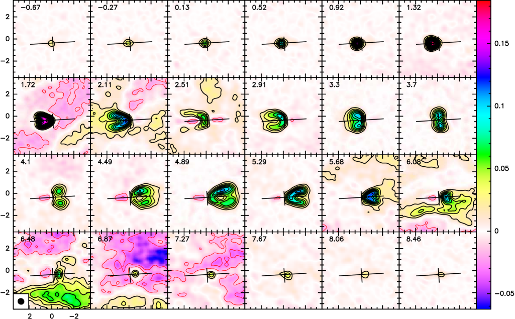
Figure 1: Channel maps of the ¹²CO J=2-1 line emission toward the Flying Saucer. Contours are in step of 15 mJy/beam (1.22 K, approx 7 $\sigma$): negative contours are in red, positive contours in black, zero level contour omitted, and the color scale is given on the right. The cross indicates the position and orientation of the dust disk. The LSR velocity (in km s^-1),is indicated in the upper left corner of each panel.

Figure 2: As Fig.1 but for the CS J=5-4 line. Contours are in step of 15 mJy/beam (1.47 K, approx 9 $\sigma$).

Imaging observations were performed with the Atacama Large mm/submm Array (ALMA) in a moderately compact configuration. The project 2013.1.00387.S was observed on 17 and 18 May 2015 under excellent weather conditions. The correlator was configured to deliver very high spectral resolution with a channel spacing of 15 kHz (and an effective velocity resolution of 40 m s${-1}$). We observed simultaneously CO J=2-1, all the most intense hyperfine components of the CN N=2-1 transition, and the CS J=5-4 line.

Data was calibrated via the standard ALMA calibration script in the CASA software package (Version 4.2.2). Titan was used as a flux calibrator. The calibrated data was regridded in velocity to the LSR frame using the “cvel” task, and exported through UVFITS format to the GILDAS package for imaging and data analysis. Atmospheric phase errors were small, providing high dynamic range continuum images and thermal noise limited spectral line data. The total continuum flux is 35 mJy at 242 GHz (with about 7% calibration uncertainty). With robust weighting, the $uv$ coverage provided by the $\sim 34$ antennas yields a nearly circular beam size close to 0.5^′′. The CS images were produced at an effective spectral resolution of 0.1 km s^-1; the rms noise is 3 mJy/beam, i.e. about 0.27 K given the beam size of $0.48^{\prime\prime}\times 0.46^{\prime\prime}$ at PA $53^{\circ}$. For CO, a spectral resolution of 0.08 km s^-1 was used, and the rms noise is 4 mJy/beam, i.e. about 0.37 K given the beam size of $0.51^{\prime\prime}\times 0.48^{\prime\prime}$ at PA $54^{\circ}$.

Figures 1 and 2 present the CO and CS channel maps, respectively, spectrally smoothed to a $0.4\,\,{\rm km\,s}^{-1}$ for clarity. Figure 3 is a summary of the emission from CO, CS and the dust continuum.

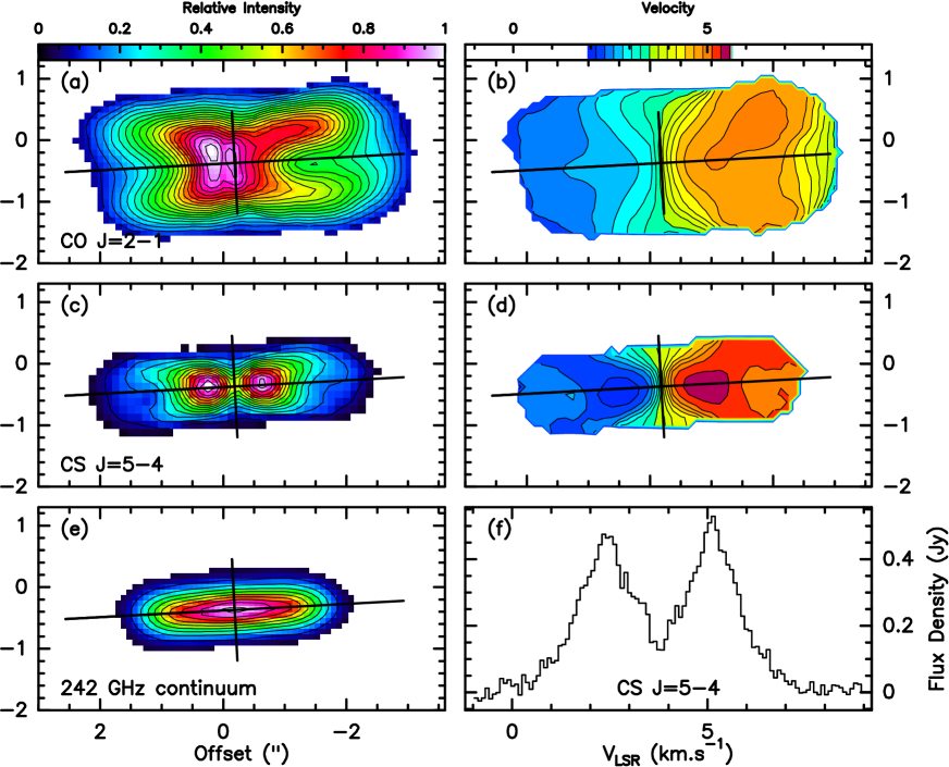
Figure 3: A summary of the observations for CO, CS and dust. CO J=2-1 integrated intensity map (a) and isovelocity contours (b), CS J=5-4 integrated intensity map (c) and isovelocity contours (d), continuum image at 242 GHz (e) and CS J=5-4 integrated spectrum (f).

In addition, a CO J=2-1 spectrum of the clouds along the line of sight was obtained with the IRAM 30-m telescope, as described in Guilloteau et al. (2016).

3 Results

The CO J=2-1 and continuum results were partially reported by Guilloteau et al. (2016), who used them to measure the dust temperature.

3.1 Images

Figure 3 clearly shows that the disk is viewed close to edge-on. It also reveals a vertical stratification of the dust and molecules.

The modeling of the continuum image by Guilloteau et al. (2016) leads for the (millimeter) dust grains to a scale height of $12.7\pm 0.3$ au at 100 au, increasing with a $0.34\pm 0.04$ exponent. For comparison, the modeling of the near-infrared images by Grosso et al. (2003) leads for the (micron) dust grains to a larger scale height of $22.5\pm 1.5$ au at 100 au when adopting the same definition and distance, and increasing more rapidly with a 1.25 exponent. Therefore, there is a clear indication of dust settling in this disk, with large grains preferentially close to the disk mid-plane.

The integrated intensity maps (Fig.3) show that CS is significantly more confined towards the disk mid-plane than CO. As mentioned in Guilloteau et al. (2016), CO is contaminated by background emission from extended molecular clouds at four different velocities, which affect the derivation of the integrated emission and result in apparent asymmetries. The CS molecular emission extends at least up to radius of about 300 au, and slightly more ($\sim 330$ au) for CO. On the contrary, the dust emission is confined within 200 au. The apparent distributions may be more a result of temperature gradients, excitation conditions and line opacities than reflecting different abundance gradients for these molecules. The CO J=2-1 line is much more optically thick than the CS line, and thus more sensitive to the (warmer) less dense gas high above the disk mid-plane. Along the mid-plane, self-absorption by colder, more distant gas, can result in lower apparent brightness. However, at the disk edges, this effect should be small, so the higher brightness above the disk plane likely indicates a vertical temperature gradient, with warmer gas above the plane.

The aspect of the iso-velocity contours (Fig.3) is exactly what is expected from a Keplerian flared disk seen edge-on. In such a configuration, at an altitude $z$ above the disk plane, the disk only extends inwards to an inner radius depending on $z/H$, where $H$ is the scale height, so that the maximum velocity reached at altitude $z$ is limited by this inner radius. Thus the mean velocity decreases from the mid-plane to higher altitude, resulting in the “butterfly” shape of the iso-velocity contours. The effect is however less pronounced for CO, as its high optical depth allows us to trace the emission well above the disk plane (iso-velocity contours would be parallel for a cylindric distribution).

3.2 Simple determination of the disk parameters

To constrain the basic parameters of the disk, we make a simple model of the CS J=5-4 emission with DiskFit (Piétu et al. 2007) assuming power laws for the CS surface density ($\Sigma_{CS}(r)=\Sigma_{0}(r/\mathrm{100au})^{-p}$) and temperature $T_{ex}(r)=T_{0}(r/\mathrm{100au})^{-q}$. The disk is assumed to have a sharp outer edge at $R_{\mathrm{out}}$. The vertical density profile is assumed Gaussian (see Eq.1 Piétu et al. 2007)), with the scale height a (free) power law of the radius: $h(r)=H_{0}(r/\mathrm{100au})^{-h}$. The line emission is computed assuming a (total) local line width $dV$ independent of the radius and LTE (i.e. $T_{0}$ represent the rotation temperature of the level population distribution).

Besides the above intrinsic parameters, the model also includes geometric parameters: the source position $x_{0},y_{0}$, the inclination $i$ and the position angle of the rotation axis $PA$, and the source systemic velocity $V_{\mathrm{LSR}}$ relative to the LSR frame.

Results are given in Table 1. This simple model allows us to determine the overall disk orientation, the systemic velocity and the stellar mass, and gives an idea of the temperature required to provide sufficient emission. The apparent scale height $H_{0}$ derived at 100 au would correspond to a temperature of 53 K, much larger than $T_{0}$. The difference may indicate that CS is substantially sub-thermally excited or, more likely, that CS emission only originates from above one hydrostatic scale height.

Table 1: CS disk modeling results.

Parameter	Value (at 100 au)	Unit
$PA$	$3.6\pm 0.4$	∘	PA of disk rotation axis
$i$	$85.4\pm 0.5$	∘	Inclination
$V_{\mathrm{LSR}}$	$3.755\pm 0.003$	km s-1	Systemic velocity
$M_{*}$	$0.58\pm 0.01$	$\,\mathrm{M}_{\odot}$	Star mass (a)
$R_{\mathrm{out}}$	$290\pm 7$	au	Outer radius
$dV$	$0.17\pm 0.01$	km s-1	Local line width (b)
$\Sigma_{0}$	$4.3\,10^{13}\pm 0.3\,10^{13}$	cm-2	CS Surface density
$p$	$2.71\pm 0.03$		Surface density exponent
$T_{0}$	$18.0\pm 0.5$	K	CS temperature
$q$	$-0.18\pm 0.03$		temperature exponent
$H_{0}$	$25.8\pm 0.3$	au	Scale height of CS (c)
$h$	$-1.40\pm 0.03$		exponent of scale height

(a) Assuming Keplerian rotation. (b) assumed constant with $r$. Errors are formal errorbars from the fit. (c) apparent scale height (see section 3.2).

3.3 PV-diagrams

A more detailed understanding of the disk properties can be derived from the position-velocity diagram shown in Figures 4 and 5 where several altitudes $z$ are shown. In such diagrams, radial straight lines (i.e. lines with $v(x)-V_{\mathrm{disk}}\propto x$, where $x$ is the impact parameter, $v$ the velocity and $V_{\mathrm{disk}}$ the disk systemic velocity) trace a constant radius $r$ (see Appendix The Flying Saucer: Tomography of the thermal and density gas structure of an edge-on protoplanetary disk. for details). The blue straight lines indicate the outer radius ($R_{\mathrm{out}}\simeq 330$ au). The blue curve is the Keplerian rotation curve $\sqrt{GM_{*}/r}$, with a stellar mass of $0.57\,\mathrm{M}_{\odot}$. The black line is the apparent inner radius $R_{\mathrm{in}}$, and white-over-black line delineates the radius $r_{\mathrm{dip}}\simeq 185\,\mathrm{au}$, where a dip in emission is observed at low altitudes both in CO and in CS.

The CO J=2-1 line provides a direct view into the thermal structure of the disk. Like for the continuum emission, the background provided by the four extended molecular clouds identified in the 30-m spectrum modulates the apparent brightness of the disk, since the ALMA array only measures the difference in emission between the disk and the background clouds. Because the CO J=2-1 line is essentially optically thick in disks, we can simply recover a corrected CO PV diagram by adding the background spectrum obtained with the IRAM 30m, (see Guilloteau et al. 2016, their Fig.1) to the observed CO emission, at least within the disk boundaries (in position and velocity). The result is given in Fig.4 (bottom).

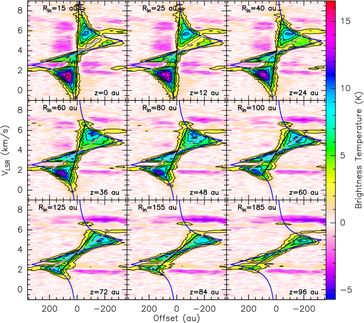
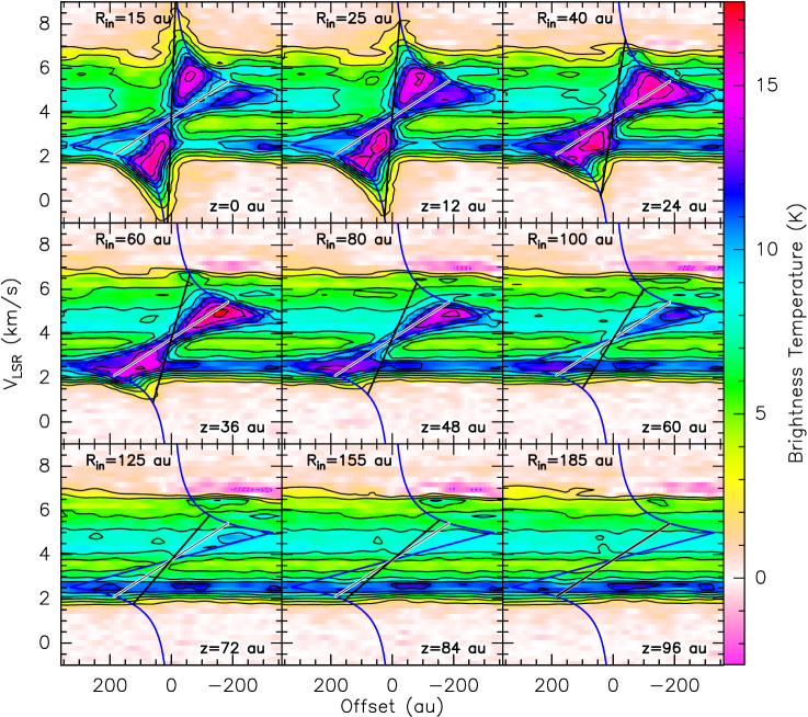
Figure 4: Position - Velocity diagram for CO J=2-1. Each panel is a cut at a different height above the plane (indicated in the lower right corner of each panel). The spatial resolution is 56 au. Top: without the background added (spectral resolution 0.08 km s^-1). Bottom: with the background spectrum added. On each panel, the black line highlights the apparent inner radius whose value is quoted in the upper left corner. Here, the spectral resolution is 0.27 km s^-1.

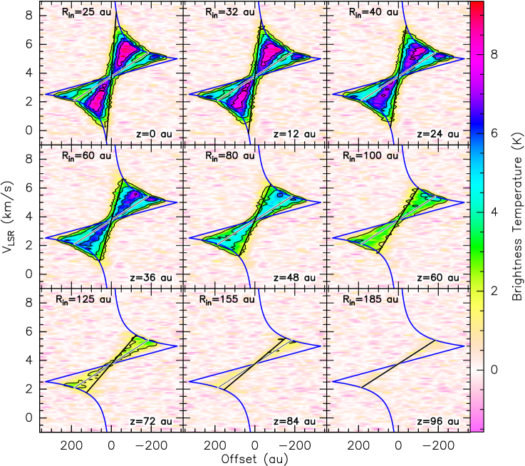
Figure 5: As in Fig.4, but for CS J=5-4 (spectral resolution 0.10 km s^-1).

In the disk plane, while CO appears to extend down to very small radii ($<15$ au), CS may have an inner radius around 25 au.

At a given location, the impact of the finite beamsize depends on the brightness temperature gradients which are different for CO and CS (because of different opacities and excitation conditions) leading therefore to different apparent structures. Nevertheless, all apparent inner radii increase with height above the disk plane, as described before for the analysis of iso-velocity curves. This happens because the disk is flaring due to the hydrostatic equilibrium, hence its vertical thickness is increasing with radius.

The disk mid-plane is also clearly colder than the brightest background molecular cloud at 2.8 km s^-1, which has $J_{\nu}(T)=11$ K, beyond about 100 au radius, being almost as warm as the second brightest cloud at 4.2 km s^-1, with $J_{\nu}(T)=8$ K, at radii around $185\,\mathrm{au}$. From this simple consideration, we safely constrain the mean disk mid-plane temperature, averaged over one beam, to be 13 K near 180 au, after proper conversion of the brightness temperature outside of the Rayleigh-Jeans domain. It would rise to about 18 K at 100 au.

The PV diagrams above the disk plane indicate a warmer temperature in the upper layers, since no absorption is visible for $z>40$ au or so. Because of our limited linear resolution (about 56 au), with such a vertical temperature gradient the CO PV diagram only gives an upper limit to the disk mid-plane temperature because the scale height (about 10 au at 100 au) is substantially smaller than the linear resolution except at the disk edge.

We also note that both CS and CO shows a drop in the emission intensity at radius $r_{\mathrm{dip}}\simeq 185\,\mathrm{au}$. This drop is somewhat more difficult to identify in the CO PV diagrams because of the background clouds. In CO, the emission drop seems to disappear at an height of 40 au, suggesting it occurs only below about 30-40 au given the limited angular resolution. Beyond a radius of 220 au, CO emission is observed again. In CS, the deficit of emission near $185\,\mathrm{au}$ extends somewhat higher, up to a height of 60 au.

Figure 6 also reveals a north-south asymmetry, the north side being brighter in CS and in CO.

4 A new method of Analysis

4.1 Deriving the brightness distribution from the PV-diagram

For an homogeneous medium, the measured brightness temperature $T_{b}$ is given by

$$T_{b}=(1-\exp(-\tau))(J_{\nu}(T)-J_{\nu}(T_{bg}))$$ (1)

where $J_{\nu}$ is the Planck function multiplied by $c^{2}/2k\nu^{2}$,

$$J_{\nu}(T)=\frac{h\nu}{k}\frac{1}{\exp(h\nu/(kT))-1}.$$ (2)

Since in a PV diagram a radial line represents a constant radius, we can recover the disk temperature from the thermalized and optically thick CO J=2-1 transition by averaging the observed brightness along such radial lines in regions where the signal is sufficiently resolved spectrally and spatially. This averaging process yields the mean radiation temperature, $J_{\nu}(T)-J_{\nu}(T_{\mathrm{bg}})$, from which the temperature $T$ is derived. The disk being seen edge-on, cuts at various altitudes $z$ provide a direct visualisation of the gas temperature versus radius $T(r,z)$, although only at the angular resolution of the observations. The 2-D image resulting from the application of this averaging process is called hereafter the tomographically reconstructed distribution or TRD.

While the CO J=2-1 TRD is just the temperature distribution, for optically thinner or non thermalized lines, the interpretation is more complex because the TRD is a function of both the temperature and local density. Nevertheless, it also provides a direct measurement of the altitude of the molecular layer.

We use the PV-diagrams of CO and CS transitions to derive their respective TRDs and show them in Fig. 6. The derivations were performed onto data cubes without continuum subtraction because the subtraction, which was needed to compute the iso-velocity contours, may lead to substantial problems near the peak of the continuum. For CO, which is optically thick, the TRD$(r,z)$ map is obtained using the PV-diagram with the CO emission from the background clouds added, since that emission is fully resolved out by the ALMA observations. This explains why the derived CO temperature brightness is of the order of 15 K around the disk, in agreement with the values derived from the CO spectrum taken with the IRAM 30-m radiotelescope (Guilloteau et al. 2016).

In each case, we calculated a map of the mean, median and maximum brightness along each radius. For CO, the mean and maximum brightness are contaminated by the background clouds, and the median is expected to be a better estimator. Furthermore, for CS, we found that the mean and the median always give results which differ by less than 1 K inside the disk at $r<350$ au (see Fig.6, panel (d) which shows the difference between the mean and the median for CS 5-4). This indicates that the derivations are robust and do not suffer from significant biases. The observed TRDs clearly confirm the location of the molecular layer above the mid-plane but the CS emission peaks at a lower temperature and is located below the CO emission. The ratio of the CS TRD over the CO TRD confirms these behaviors (see panel (a) of Fig.6).

The Keplerian shear implies that the spatial averaging of the derived brightness is not the same everywhere inside the disk. Indeed, at a radius $r$ corresponding to a velocity $v(r)$, the smearing due to the Keplerian shear is given by $dr=2rdv/v(r)$ where $dv$ is the local linewidth, which is due to a combination of thermal and turbulent broadening. This limits the radial resolution which can be obtained in the disk outer parts. For instance, for CO, at 20 au, assuming a temperature of 30 K and a turbulent boadening ($0.05\,{\rm km\,s}^{-1}$) similar to that observed in TW Hydrae disk by Teague et al. (2016), the $dr$ would be of the order of $\sim 2$ au, a value which would not affect studies at spatial resolution down to $0.1^{\prime\prime}$ (12 au) or so. On the contrary, at radius 200 au, the $dr$ would be of the order of 35 au for the same line width, dropping to 20 au assuming the same turbulence but a (mid-plane) temperature of 7 K. This limits the gain obtained with high angular resolution only at large radii. It also explains why the apparent extent of the tomographically reconstructed distribution in Fig.6 exceeds the disk outer radius more than expected from the angular resolution only.

Nevertheless, this smearing is purely radial and the vertical structure is not affected: the smearing is the same above and below the mid-plane at a given radius (assuming there is no vertical temperature gradient).

This occurs because the disk is edge-on but it is no longer true in less inclined disks. In such disks, the smearing resulting from the local line width will limit the effective resolution radially and vertically.

Finally, we note that this direct method of analysis, specific to edge-on disks, is complementary to the classical channel maps studies by providing a more synthetic but direct view of the vertical disk structure.

Figure 6: Derivations of the gas temperature from the PV-diagram. (a) ratio of the median TRD derived from CS over the median TRD derived from CO (contours are 0.1 to 1 by 0.1) (b) CO median TRD, with contours from 4 to 22 K by spacing of 2 K. (c) CO median TRD with contours of the CS median TRD overlaid. (d) difference between the CS mean temperature and the CS median TRD (contours are from -0.6 to 0.6 K by spacing of 0.3 K). (e) median CS TRD with contours from 4 to 12 K by spacing of 2 K. (f) CS median TRD with contours of the CO median TRD. The spatial resolution is indicated. The vertical line delineates the area suffering from beam dilution.

4.2 CO Modeling using DiskFit

To go beyond the resolution-limited information provided in Fig.6, we study here the impact of several key parameters of the disk by performing grids of models to better constrain the disk geometry and structure. We use the ray-tracing model DiskFit (see Section 3.2, Piétu et al. 2007). For simplicity, we assume LTE conditions, which is appropriate for CO. The temperature structure is here more complex than the simple vertically isothermal model of Section 3.2. The atmosphere temperature is given by

$$T_{atm}(r)=T_{atm}^{0}\left(\frac{r}{r_{0}}\right)^{-q_{atm}}$$ (3)

and the mid-plane temperature is given by

$$T_{mid}(r)=\min\left(T_{atm}(r),T_{mid}^{0}\left(\frac{r}{r_{0}}\right)^{-q_{mid}}\right)$$ (4)

In between for an altitude of $z<z_{q}$ , the temperature is defined by

$$T(r)=\left(T_{atm}(r)-T_{mid}(r)\right)\left(\cos\left(\frac{\pi z}{2z_{q}H(r)}\right)\right)^{2\delta}+T_{mid}(r)$$ (5)

where $H(r)$ is the hydrostatic scale height (defined by $T_{mid}(r)$). Provided $q_{atm}>q_{mid}$, there is a radius $R_{q}$ beyond which the temperature becomes vertically isothermal. Note that for $q_{mid}=0$, this definition is identical to that used by Dartois et al. (2003).

The models of the molecular emission were performed together with the continuum emission not subtracted. The continuum model uses, in particular for the density and temperature, the parameters defined in Table 1 of Guilloteau et al. (2016). We take into account the spatial resolution by convolving all models by a $0.5^{\prime\prime}$ circular beam. In all models, the outer radius $r_{out}$ is taken at 330 au, in agreement the value derived from the PV-diagram.

We find that a small departure from edge-on inclination by 2-3 degrees is sufficient to explain the small North-South brightness asymmetry visible in Fig.6. The most probable value is $i=87^{\circ}$ (see Sect.5.1), a value used for all further models.

In a first series of models, we assume a CO vertical distribution which follows the H₂ density distribution, i.e. assuming a constant abundance. For the H₂ density distribution, we assume either power laws or exponentially tapered distribution following the prescription given in Guilloteau et al. (2011). We explored CO surface densities ranging from 10¹⁶ to 10¹⁹ cm^-2 at 100 au. To account for the observed brightness at high altitudes above the disk plane, we find that the CO surface density at 100 au must be at least of the order of 5 $10^{17}$ cm^-2, with a power law index of the order of $p=1.2$ for the radial distribution. We also explored the impact of the temperature distribution $z_{q}$, $\delta$, $T_{atm}^{0}$, $q_{atm}$, $T_{mid}^{0}$, $q_{mid}$ and $R_{q}$. Best runs are obtained for mid-plane temperatures $T_{mid}\approx 10$ K at 100 au, $q_{mid}=0.4$ leading to about 6 K at the outer disk radius and 17 K at 26 au (CO snowline location), $T_{atm}^{0}=$50 K, $q_{atm}=0-0.2$, $\delta=2$ and $z_{q}=1.3-2$.

However none of these models, which assume CO molecules are present everywhere in the disk, properly reproduce the CO depression observed around the mid-plane (see panel (b) of Fig.6). This remains true even if the mid-plane temperature is set to values 5-7 K, matching the temperature of large grains measured by Guilloteau et al. (2016).

We attempted to perform more realistic models by assuming complete molecular depletion (abundance $X_{p}(\mathrm{CO})=0$) in the disk mid-plane. In this model, the zone in which CO is present is delimited upwards by a depletion column density $\Sigma_{dep}$ and downwards by the CO condensation temperature. CO molecules are present (with a constant abundance $X_{u}(\mathrm{CO})=10^{-4}$) when the H₂ column density from the current $(r,z)$ point upwards (i.e. towards ($r,\infty$)) exceeds a given threshold $\Sigma_{dep}$, to reflect the possible impact of photo-desorption of molecules, or when the temperature $T(r,z)$ is above 17 K. Such a model takes into account the possible presence of CO in the inner disk mid-plane inside the CO snowline radius, and also at large radii because as soon as the surface density becomes low enough, CO emission can again be located onto the mid-plane. In this model, the CO surface density radial profile $\Sigma(r)\times X_{u}(\mathrm{CO})$ (where $\Sigma(r)$ is the H₂ surface density profile) is constrained, because of the need to provide sufficient opacity for the CO J=2-1 at high altitudes above the disk mid-plane to reproduce the observed brightness. The derived H₂ densities are then strictly inversely proportional to the assumed $X_{u}(\mathrm{CO})$.

Table 2 gives the parameters of the best model we found with this approach. Unfortunately the current angular resolution of the data limits the analysis. Because of this limited angular resolution, parameters $T_{atm}^{0},\delta,z_{q}$ are strongly coupled. $z_{q}$ also depends implicitely on $T_{mid}$, because it is the number of hydrostatic scale heights at which the atmospheric temperature is reached. In practice, Table 2 only confirms a low mid-plane temperature ($10$ K at 100 au), and temperatures at least a factor 2 larger than this in the CO rich region, consistent with the (spatially averaged) values derived in Section 3.3. Only higher spatial resolution data would allow us to break the degeneracy and accurately determine the vertical temperature gradient (see Section 5.4).

Furthermore, even this model only qualitatively reproduces the brightness distribution of the CO emission around the mid-plane. In particular, the shape of the depletion zone is difficult to evaluate from the current data. We also fail to reproduce the rise of the CO brightness after 250 au, most likely because our model does not include an increase of the temperature in the outer part.

Most chemical models (e.g. Reboussin et al. 2015) predict that there is some CO at low abundance ($X_{p}(\mathrm{CO})\sim 10^{-8}-10^{-6}$) in the mid-plane, depending on the grain sizes and the local dust to gas ratio, contrary to our simple assumption of $X_{p}(\mathrm{CO})=0$. Such low abundances would not impact our determination of the CO surface density, which only relies on the need to have sufficient optical thickness in the upper layers. However, CO could start being sufficiently optically thick around the mid-plane, diminishing the contrast between the mid-plane and the molecular layer. We estimated through modelling that this happens for $X_{p}(\mathrm{CO})\geq 3\,10^{-8}$. In such cases, the brightness distribution becomes similar to that of the undepleted case. Observations of a less abundant isotopologue would be a better probe of the mid-plane depletion.

We thus conclude that the current data are insufficient to disentangle between molecular depletion and a very cold mid-plane, but indicate a rise in mid-plane temperature beyond 200 au.

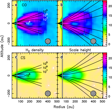
Figure 7: Superimposition of the CO and CS median TRD to a standard disk model. (a): CO TRD (colour) and the H₂ volume density superimposed in labelled contours from $10^{5}$ up to $10^{8}$ cm^-3. (b): CO TRD with the scale height superimposed in black contours from 1 to 4 scale heights. (c) and (d) as (a) and (b) but for CS. The model corresponds to the parameters given in the Table 2.

In Fig. 7, we overlay the brightness temperature derived from the observations to the structure of the model given in Table2. The brightness temperature from the model is compared to the observations and also shown in Fig. 8 at three different angular resolutions of $0.5^{\prime\prime},0.3^{\prime\prime}$ and $0.1^{\prime\prime}$.

Table 2: Model derived from the CO observations

Parameter	Value	Unit	Parameters at 100 au
$T_{atm}^{0}$	50	K	Atmosphere temperature
$q_{atm}$	0.4
$z_{q}$	3
$\delta$	2
$T_{mid}^{0}$	10	K	Mid-plane temperature
$q_{mid}$	0.4
$\Sigma_{0}$	$10^{23}$	cm-2	H2 Surface density
$p$	$0.5$		Surface density parameter
$R_{C}$	$50$	au	Radius for exponential decay
$H_{0}$	11.3	au	Scale height
$h$	-1.3		exponent of scale height
$R_{\mathrm{out}}$	$330$	au	Outer radius
$i$	$87$	∘	Inclination
$\Sigma_{dep}$	$10^{22}$	cm-2	Surface density for depletion
$T_{dep}$	17	K	Depletion temperature
$X_{u}($CO$)$	10-4		CO abundance in upper layers
$X_{p}($CO$)$	0		as above, in mid-plane
$M_{\mathrm{disk}}$	$0.7\,10^{-3}$	$\,\mathrm{M}_{\odot}$	Disk mass

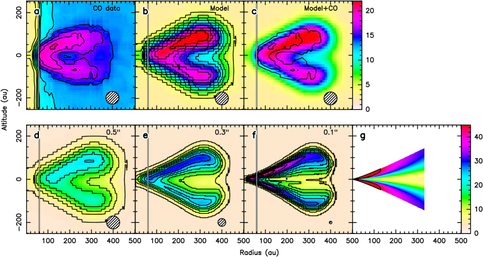
Figure 8: TRD for CO J=2-1 (in Kelvin). (a) observed CO TRD. (b) best model. (c) CO TRD in false color with best model in black contours. (d) model at $0.5^{\prime\prime}$ or 60 au resolution, (e) at $0.3^{\prime\prime}$ or 36 au resolution and (f) at $0.1^{\prime\prime}$ (12 au) resolution, presented with the same color scale. Contours are in 4 K steps. (g) Initial temperature distribution; the black contour is at 45 K.

5 Discussion

5.1 Overall disk structure

The analysis of the CO and CS brightness temperature patterns shows that there is no significant departure from a simple disk geometry at the linear resolution of 60 au, with the exception of the North-South brightness difference. This may be due to an intrinsic assymetry. However, the same effect can also be produced if the disk is slightly inclined by a few degrees from edge-on. Due to the flaring and radial temperature gradient, the optically thick emission of the far side always originates from slightly warmer gas Guilloteau & Dutrey (1998). Indeed, we find that an inclination angle of 87^∘ is enough to account for the North-South dissymmetry, with the Southern part of the disk being closer to us. This inclination (and orientation) is in very good agreement with that of $86\pm 1^{\circ}$ derived by Grosso et al. (2003) from near InfraRed (NIR) observations. The brightness distributions of the NIR images also show that the southern part of the disk is closer to us. Finally, there is no apparent sign of warp beyond a radius of about 50 au.

Figure 7 shows the CO emission is above one scale height, while the CS emission appears slightly below and less extended vertically. This is not surprising. CS J=5-4 is excited only at the high densities near the mid-plane while CO J=2-1 is easy to thermalize at density as low as a few 10³ cm^-3 (see panels a-c of Fig.7 which trace the density distribution). As a consequence, the convolution by the $\sim 56$ au beam leads to different positions of the peak of the emission layer. The CO layer is vertically resolved and extended, while the CS emission is vertically unresolved and peaks just below one scale height. These vertical locations for the CO and CS layers are consistent with predictions by chemical models (see Dutrey et al. 2011, Fig. 8 where CS peaks between 1 and 2.5 scale heights). A CO layer above the mid-plane was already observed in the disk of HD 163296 (de Gregorio-Monsalvo et al. 2013; Rosenfeld et al. 2013).

We also estimate for the first time the amplitude of the vertical temperature gradient between the cold mid-plane, the molecular layer and CO atmosphere at radii between 50 and 300 au. The gas vertical temperature gradient which is derived at 100 au is in agreement with that predicted by thermo-chemical models (e.g. Cleeves et al. 2016) with a mid-plane at about 8-10 K and a temperature of 25 K reached at two scale-heights. The main limitation here is the linear resolution of 60 au. Nevertheless, the observed pattern of the brightness distribution suggests the existence of warmer gas inside a radius of about 50-80 au. Any inner hole of radius $<15$ au cannot be seen in these data due to our sensitivity limit.

5.2 Radial profile of CO near the mid-plane

Rise of the CO brightness a large radius:

While in the upper layers, the CO brightness decreases smoothly with radius, in the mid-plane, we observe a rise in CO brightness beyond a radius of about 200 au. The transition radius coincides with the mm-emitting dust disk outer boundary, $\sim 187$ au in the simple model from Guilloteau et al. (2016), while in scattered light, the disk is nearly as extended as the CO emission (Grosso et al. 2003). This suggests that a change of grain size distribution may also play a role here. With the dust composed of mostly micron-sized grains better coupled with the gas (see Pontoppidan et al. 2007), more stellar light may be intercepted, resulting in a more efficient heating of the gas, as suggested by recent chemical models (Cleeves 2016). Moreover, at the expected densities in the disk mid-plane, the dust and gas temperatures should be strongly coupled, and a dust temperature rise is also naturally expected when the disk becomes optically thin to the incident radiation and for the re-emission, as shown e.g. by D’Alessio et al. (1999).

Also, as the $\rho$ Oph region is bathed in a higher-than-average UV field due the presence of several B stars, this effect may be reinforced by additional heating due to a stronger ambient UV field. However, the Flying Saucer is located on the Eastern side of the dark cloud, whose dense clouds absorb the UV from the B stars, located mainly on the Western side. Fig. 1a and 4a of Lim et al. (2015) show that there is a clear dip in the FUV emission due to the dark cloud silhouette. Therefore at the location of the Flying Saucer (l=353.3, b=16.5) the ambient FUV field cannot be very large.

Apparent gap at radius $185\,\mathrm{au}$:

The presence of an apparent gap at $\sim$ 185 au both in CO and CS is puzzling. Its existence in CO however indicates that a change in temperature and/or beam dilution is the primary cause for this deficit, as CO is easily thermalized and optically thick. This suggests that the disk mid-plane warms up beyond this radius, before the emission fades again near the disk edge (of the order of $\sim$ 330 au), where CO becomes optically thin and CS unexcited.

An alternative explanation is that it is the result of real gap in the molecular distribution, smoothed out by our limited angular resolution. The optically thick CO line traces material both at low and high altitude (up to 3-4 scale heights above the mid-plane) while CS J=5-4, a high density tracer, is more optically thin and only observed in high density regions (at typically one scale height). Contrary to a face-on or inclined disk, the gap can be seen in ¹²CO because the disk is edge-on.

The brightness minimum at $185\,\mathrm{au}$ is only seen at low altitudes, typically between the mid-plane and an altitude of 40 au in CO, and slightly higher in CS, so the putative gap cannot extend up in the disk. This morphology remains consistent with expectations for gaps created by planets, provided the Hills radius is smaller than the disk scale height.

5.3 Deriving the gas density from CS excitation conditions

In CS J=5-4, we observe a similar North-South asymmetry than in CO J=2-1. This indicates that the emission has a substantial optical thickness along the line of sight.

The brightness ratio of CS over CO is within the range 0.5-0.7 until a radius of about 250 au and drops quickly beyond. As indicated by the iso-density contours shown in Figure 7, this is consistent with the decreasing H₂ density with radius, because the CS J=5-4 transition is thermalized at a few $10^{6}$ cm^-3 (Denis-Alpizar et al. 2017).

On the contrary, the observed ratio of 0.5-0.7 in the inner disk mid-plane cannot be explained by excitation conditions. A simple LVG calculation using the CO freeze out temperature $T_{k}=17$ K (which is in agreement with the CS temperature derived from the simple analysis), a surface density of $4\,10^{13}$ cm^-2 and a local line width of 0.3 km s^-1 (obtained from a simple analysis with DiskFit using a power law surface density distribution) yields $T_{ex}=12$ K for a density of $10^{6}$ cm^-3. This density is much lower than expected in the disk given the dust emission observed at mm wavelengths, and than the values derived from our CO modelling.

The ratio is better explained as resulting from different beam dilutions in CO and CS. At 200 au, while the CO emission is spatially resolved, the region emitting in CS J=5-4 must fill only 50% of the synthesized beam, i.e. must have a thickness of only $\sim 30$ au. The emission peak being located $\sim 45$ au above the plane at this radius, the CS emitting layer must be confined between about 30 and 60 au there. Furthermore, the density at $r=200$ au and $z=60$ au is about $10^{6}$ cm^-3 in our fiducial disk model, so that the upper layers are no longer dense enough to excite the J=5-4 line. Hence the observed CS/CO brightness ratio is roughly consistent with a molecular layer extending above one scale height, with sub-thermal excitation of the CS J=5-4 transition truncating the CS brightness distribution upwards.

In this interpretation, the CS layer is expected to be thinner for higher J transitions. An angular resolution around $0.2^{\prime\prime}$ would be needed to resolve the CS layer.

At smaller radii, the CO and CS layer become both unresolved vertically, but the ratio of their respective thickness is not expected to change significantly, leading to the nearly constant brightness ratio.

5.4 Limits: angular resolution, local line width and inclinations.

Figure 8 shows the TRD of the model obtained with DiskFit assuming CO depletion around the mid-plane at 3 different angular resolutions, $0.5^{\prime\prime}$, $0.3^{\prime\prime}$ and $0.1^{\prime\prime}$. The impact of the resolution on this apparent brightness distribution is striking. For comparison, the intrinsic temperature $T(r,z)$ distribution is shown in panel (g) for all points where the H₂ density exceeds $10^{4}$ cm^-3. Comparing panels (f) and (g) shows the impact of the small Keplerian shear compared to the local line width at the disk edge (which spreads the TRD beyond the outer disk radius, see Section 4.1), and of the small deviation from a pure edge-on disk (which result in a top/bottom asymmetry). For this specific disk structure, the peak brightness is lowered by a factor 2 when degrading the angular resolution from $0.1^{\prime\prime}$ to $0.5^{\prime\prime}$. The inner CO disk, the radius of the CO snowline and the whole gas distribution can be resolved at $0.1^{\prime\prime}$, but not at $0.5^{\prime\prime}$. The stratification of the molecular layer can only be studied at $0.1^{\prime\prime}$ resolution, down to about 30 au, where the scale height becomes too small compared to the linear resolution for a direct measurement. We also observe a displacement of the peak brightness towards larger radii at $0.5^{\prime\prime}$ resolution compared to its (true) location at $0.1^{\prime\prime}$ resolution. This is due to the fact that the vertical extent of the CO emission at large radii is larger due to the flaring. Finally, at $0.5^{\prime\prime}$, we find that it is not possible to determine the shape of the (partly) depleted zone around the mid-plane beyond the CO snowline radius. Even a resolution of $0.3^{\prime\prime}$ would allow the measurement of the depletion factor (and estimate of the CO/dust ratio) around the mid-plane while an angular resolution of $0.1^{\prime\prime}$ would in addition provide the determination of the shape of this area.

Besides angular resolution and local line width, inclination is another limitation of the method. To first order, the disk should be edge-on to within about $h(r)/r$ for the TRD to be directly useable, i.e. in the range $80-90^{\circ}$ given the typical $h(r)/r$ of disks at 100-300 au. However, even for somewhat lower inclination, the TRD can give insight onto the location of the molecular layer. We illustrate this in Appendix B.

Such simulations clearly demonstrate how powerful ALMA can be to characterize the structure of an edge-on protoplanetary disk, provided its distance is reasonable.

6 Summary

We report an analysis of the CO J=2-1 and CS J=5-4 ALMA maps of the Flying Saucer, a nearly edge-on protoplanetary disk orbiting a T Tauri star located in the $\rho$ Oph molecular cloud. At the angular resolution of $0.5^{\prime\prime}$ (60 au at 120 pc) and in spite of some confusion in CO due to the background molecular clouds, we find that:

• the disk is in Keplerian orbit around a 0.57 $\,\mathrm{M}_{\odot}$ star and nearly edge-on (inclined by $87^{\circ}$). It does not exhibit significant departure from symmetry, neither in CO nor in CS,

• direct evidence for a vertical temperature gradient is demonstrated by the CO emission pattern. Quantitative estimates are however limited by the spatial resolution.

• disentangling between CO depletion and very low temperatures is not possible because of the limited angular resolution. Models with CO depletion in the mid-plane only agrees marginally better, and the mid-plane temperature cannot be significantly larger than 10 K at 100 au.

• the CO emission is observed between 1 and 3 scale heights while the CS emission is located around one scale height. Sub-thermal excitation of CS may explain this apparent difference.

• CO is also observed beyond a radius of 230-260 au, in agreement with models predicting a secondary increase of temperature due to higher UV flux penetration in the outer disk. However, the limited angular resolution does not rule out an alternate explanation with a molecular gap near $185\,\mathrm{au}$.

Finally, our results demonstrate that observing an edge-on disk is a powerful method to directly sample the vertical structure of protoplanetary disks provided the angular resolution is high enough. At least one data set with angular resolution around $0.1-0.2^{\prime\prime}$ is needed for a source located at 120-150 pc.

Appendix A PV diagram for an edge-on Keplerian disk

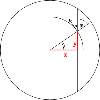
Figure 9: Definition of notations.

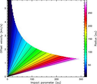
Figure 10: Radius as a function of Position and Velocity for an edge-on Keplerian disk

Let $x$ be the impact parameter in the disk, and $y$ the coordinate along the line of sight, $r$ the radial distance

$$r(y)=\sqrt{x^{2}+y^{2}}$$ (6)

where $y<y_{m}$, with $y_{m}$ given by

$$y_{m}=\sqrt{R_{d}^{2}-x^{2}}$$ (7)

The angle $\phi$ is defined such that $x=r\sin{\phi}$ (see Fig.9) The projected velocity along the line of sight is

$$V_{y}=\sqrt{GM/r}\sin{\phi}=\sqrt{GM/r}\frac{x}{r}=\sqrt{GM}\frac{x}{r^{3/2}}$$ (8)

Thus we simply recover $r$

$$r=\left[GM\left(\frac{x}{V_{y}}\right)^{2}\right]^{1/3}=R_{d}\left(\frac{X}{V}\right)^{2/3}$$ (9)

where $X=x/R_{d}$,$V=V_{y}/V_{d}$ and $V_{d}=\sqrt{GM/R_{d}}$ is the rotation velocity at the outer disk radius. Since $x\leq r\leq R_{d}$, the above equation has a solution provided $X<V<1/\sqrt{X}$ (i.e. $V_{y}>V_{d}x/R_{d}$, and $V_{y}<\sqrt{GM/x}$). So, for any given velocity $V_{y}$ and impact parameter $x$, we can solve for $r$, and then recover $y=\pm\sqrt{r^{2}-x^{2}}$ along the line of sight.

As a consequence, in the PV-diagram (showing functions of $(x,V)$) of a Keplerian disk, any line starting from ($x=0,V=V_{\mathrm{sys}}$) represent locii of constant radius. This is illustrated in Fig.10. We use this property to directly recover the temperature as a function of radius (by taking the mean or the median for any given $r$) and altitude (by making cuts in the PV diagrams for different altitudes).

For optically thick lines, this procedure yields the (beam averaged) excitation temperature, and thus the kinetic temperature if the line is thermalized.

For optically thin lines, the opacity is a function of $(r,x)$ because of the Keplerian shear which breaks the rotational symmetry. The above procedure thus yields a more complex function of the temperature and density, whose value however cannot exceed the excitation temperature at any radius $r$.

Appendix B Inclination effects

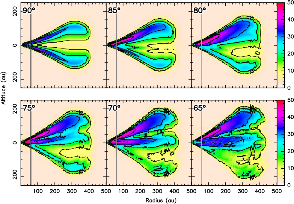
Figure 11: TRD for CO J=2-1 (in Kelvin) of our best disk model for different inclinations. Contours are in 10 K steps.

Fig.11 shows the expected TRDs of our fiducial disk model (Table 2) for different disk inclinations. Since in this model, CO emits mostly 1 or 2 scale heights above the disk mid-plane, when the inclination differs from edge-on by more $h(r)/r$, the two opposite layers can project on the same side compared to the mid-plane projection. The farthest part of the disk projects to positive altitudes in Fig.11. It appears warmer than the projection of the nearest part, because for the same impact parameter in altitude, the line-of-sight intercepts first warm gas due to the disk flaring, while for the nearest part, the warm gas is hidden behind the forefront colder regions (see Dartois et al. 2003). The depletion in the mid-plane make a clear distinction between the two emitting cones in the disk, resulting in a bright double layer at positive altitudes for $i=70-75^{\circ}$. At lower inclinations, the projected velocity gradient becomes insufficient to clearly separate these two layers on the TRD. For $i=80-85^{\circ}$, the two layers no longer project on the same side: a small lukewarm “finger” of emission appears at an altitude around $-20$ au.