Effects of local periodic driving on transport and generation of bound states

Abstract

We periodically kick a local region in a one-dimensional lattice and demonstrate, by studying wave packet dynamics, that the strength and the time period of the kicking can be used as tuning parameters to control the transmission probability across the region. Interestingly, we can tune the transmission to zero which is otherwise impossible to do in a time-independent system. We adapt the non-equilibrium Green’s function method to take into account the effects of periodic driving; the results obtained by this method agree with those found by wave packet dynamics if the time period is small. We discover that Floquet bound states can exist in certain ranges of parameters; when the driving frequency is decreased, these states get delocalized and turn into resonances by mixing with the Floquet bulk states. We extend these results to incorporate the effects of local interactions at the driven site, and we find some interesting features in the transmission and the bound states.

I Introduction

Periodically driven quantum systems have attracted an immense amount of interest for many years. A large variety of interesting phenomena resulting from periodic driving have been discovered including the coherent destruction of tunneling grossmann91 ; kayanuma94 , the generation of defects mukherjee , dynamical freezing das10 , dynamical saturation russomanno12 and localization alessio ; nag ; agarwala16 , dynamical fidelity sharma14 , edge singularity in the probability distribution of work russomanno15 and thermalization lazarides14a (for a review see Ref. dutta15, ). There have also been studies of periodic driving of graphene by the application of electromagnetic radiation gu11 ; kitagawa11 ; morell12 ; sentef15 , Floquet topological phases of matter and the generation of topologically protected states at the boundaries kitagawa10 ; lindner11 ; jiang11 ; trif12 ; gomez12 ; dora ; liu13 ; tong13 ; rudner13 ; katan13 ; lindner13 ; kundu13 ; basti13 ; schmidt13 ; reynoso13 ; wu13 ; manisha13 ; perez ; reichl14 ; manisha14 ; claassen16 ; sid17 ; hubener17 . Some of these aspects have been experimentally studied kitagawa12 ; rechtsman ; tarruell12 ; jotzu14 .

In addition, there have been several studies of the effects of interactions between electrons in periodically driven systems eckardt05 ; rapp12 ; zheng14 ; greschner14 ; lazarides14bc ; rigol14 ; ponte ; eckardt15 ; bukov16 ; lazarides14d ; keyser16 ; else ; itin15 . The effects of interactions in Floquet topological insulators have been studied in Ref. mikami16, . It is known that interactions can lead to a variety of topological phases (some of which have elementary excitations with fractional charges) in driven Rashba nanowires klino16 ; klino17 , and to a chaotic and topologically trivial phase in the periodically driven Kitaev model su16 . The effects of periodic driving on the stability of a bosonic fractional Chern insulator has been investigated raciunas16 . Interestingly some of these systems have been realized experimentally demonstrating correlated hopping in the Bose Hubbard model meinert2016 and many-body localization bordia , and realizing bound states for two particles in driven photonic systems mukherjee16 .

Periodic driving can lead to an interesting phenomenon called dynamical localization. Here the particles become perfectly localized in space due to periodic driving of some parameter in the Hamiltonian. Systems exhibiting dynamical localization include driven two-level systems grossmann91 , classical and quantum kicked rotors chirikov81 ; fishman82 ; ammann98 ; tian11 ; nieuwenburg12 , the Kapitza pendulum kapitza51 ; broer04 , and bosons in an optical lattice horstmann07 . It has been shown that remnants of dynamical localization may survive even in the presence of strong disorder roy15 .

In an earlier paper, it was shown that a combination of interactions and periodic $\delta$-function kicks with a particular strength on all the sites on one sublattice of a one-dimensional system can lead to the formation of multi-particle bound states in three different models agarwala17 . These bound states are labeled by a momentum which is a good quantum number since the system is translation invariant. This naturally leads us to ask if periodic kicks applied to only one site in a system can also lead to the formation of a bound state which is localized near that particular site. Further, it would be interesting to the effect of such a localized periodic kicking on the transmission across the site; a similar analysis for localized harmonic driving has been carried out in Refs. reyes, ; thuberg, . One can also study what happens if there is both a time-independent on-site potential (which can produce a bound state and affect the transmission on its own) and periodic kicking at the same site. Finally, one can study what the combined effect is of an interaction (between, say, a spin-up and a spin-down electron) and periodic kicking at the same site. We will study all these problems in this paper.

In one dimension it is known that periodic driving in a local region can lead to charge pumping; see Refs. agarwal07, ; soori10, and references therein. This is a phenomenon in which a net charge moves in each time period between two leads which are connected to the left and right sides of the region which is subjected to the driving. Charge pumping can happen even when no voltage bias is applied between the leads; however, this requires a breaking of left-right symmetry which can only occur if the periodic driving is applied to more than one site. In this paper, we will study the effect of driving at only site; this cannot produce charge pumping.

The plan of this paper is as follows. In Sec. II, we will introduce the basic model. We will consider a tight-binding model with spinless electrons in one dimension where periodic $\delta$-function kicks are applied to the potential at one particular site. The strength and time period of the kicks will be denoted by $\alpha$ and $T$ respectively. In Sec. III, we will discuss wave packet dynamics and how this can be used to compute the reflection and transmission probabilities across the site which is subjected to the periodic kicks. In Sec. IV, we will discuss why there is perfect reflection from the kicked site for a particular value of $\alpha$ and how this is related to dynamical localization. In Sec. V, we will show how an effective Hamiltonian can be defined and will use this to calculate the zero temperature differential conductance (which is related to the transmission probability) using the non-equilibrium Green’s function method datta . We will see that this matches the result obtained by the wave packet dynamics if $T$ is less than some value. In Sec. VI, we will discuss how the periodic kicking can lead to the formation of a state which is localized near the kicking site. If $T$ is small enough, this is a bound state, while if $T$ is large, this is a resonance in the continuum of bulk states bic ; reyes ; thuberg as we will discuss. In Sec. VII, we will see how a time-independent potential at one site affects the transmission and how periodic kicking at that site can lead to an increase in the transmission. In Sec. VIII, we will extend the model to include spin and will introduce a Hubbard like interaction between spin-up and spin-down electrons at the same site which is subjected to periodic kicks. We again study the effects of the interaction on the transmission of a two-particle wave packet dhar which is in a spin singlet state. We will also study the possibility of bound states in this system. We will end in Sec. IX with a summary of our results and some directions for future work.

II The model

We consider a chain of length $L$ on which spinless electrons hop between neighboring sites with the Hamiltonian

$$H_{TB}~{}=~{}-~{}\gamma~{}\sum_{n=1}^{L-1}~{}(c^{\dagger}_{n}c_{n+1}+H.c.),$$ (1)

where $\gamma$ is the hopping integral, and $c^{\dagger}_{n}$ and $c_{n}$ are the fermion creation and annihilation operators at site $n$ respectively. (We will set $\gamma=1$ in all our numerical calculations. We will also set the lattice spacing and $\hbar$ to 1 in this paper). The energy-momentum dispersion for this Hamiltonian is given by $E_{k}=-2\gamma\cos k$, where $k$ lies in the range $[-\pi,\pi]$; hence the group velocity is $v_{k}=|2\gamma\sin k|$. We now apply periodic $\delta$-function kicks at a single site labeled as $L_{c}$ lying in the middle of the system; the kicks are described by the time-dependent potential

$$H_{K}~{}=~{}\alpha~{}\sum_{m=-\infty}^{\infty}~{}\delta(t-mT)~{}c^{\dagger}_{L_{c}}c_{L_{c}}.$$ (2)

Hence the complete Hamiltonian (see Fig. 1) is

$$H=H_{TB}+H_{K}.$$ (3)

We are interested in studying the properties of this system as we tune parameters such as the strength $\alpha$ and the time period $T$ of the kicking.

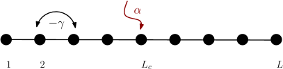
Figure 1: Schematic figure of a one-dimensional lattice where a fermion can hop between nearest-neighbor sites with amplitude $-\gamma$. A periodic $\delta$-function kick is applied at the central site $L_{c}$ of a lattice of length $L$. The kicking strength is $\alpha$.

III Wave packet dynamics and transport

We will first investigate the effect of the kicking on the transport properties. To this end, we first construct an initial wave packet at time $t=0$ given by

$$\psi_{i}(r)~{}=~{}\frac{1}{(2\pi\sigma^{2})^{1/4}}~{}\exp\Big{(}-\frac{(r-L_{o})^{2}}{4\sigma^{2}}~{}+~{}ik_{c}r\Big{)},$$ (4)

which satisfies $\int dr|\psi_{i}(r)|^{2}=\sum_{n}|\psi_{i}(n)|^{2}=1$. Here $\sigma$ denotes the width of the wave packet in real space, $k_{c}$ is the central value of the wave vector of the wave packet, and $L_{o}$ is the position in real space where the wave packet is initially centered. Since the wave packet is centered at the momentum $k_{c}$ we know that the effective group velocity of the packet will be $|2\sin k_{c}|$. We evolve the system for a time $(L-2L_{o})/|2\sin k_{c}|$; this allows the wave packet the time to travel a distance $L/2-L_{o}$ when it reaches the site where the periodic kicks are applied and then allows the transmitted part of the wave packet to travel further by an equal distance $L/2-L_{o}$. At the end of that time, we have a wave function $\psi_{f}$; we then define the transmission and reflection probabilities $\cal T$ and $\cal R$ as

$${\cal R} = \sum_{n=1}^{L_{c}}~{}|\psi_{f}(n)|^{2},\notag$$ (5)

$${\cal T} = \sum_{n=L_{c}+1}^{L}~{}|\psi_{f}(n)|^{2}.$$ (6)

These definitions ensure that ${\cal R}+{\cal T}=1$. (For spinless electrons, the transmission probability ${\cal T}$ at an energy $E$ is related to the zero temperature differential conductance $G=dI/dV$ as $G(E)=(e^{2}/h){\cal T}(E)$. In our figures, we will plot $G$ rather than $\cal T$, since $G$ is a directly measurable physical quantity). The numerical results for $k_{c}=\pi/2$ are shown in Fig. 2. (A reason for choosing $k_{c}=\pi/2$ is that this minimizes the rate of spreading of the wave packet seshadri . In one dimension, it is known that the width of a wave packet spreads in time at a rate which is proportional to $(\partial^{2}E_{k}/\partial k^{2})_{k=k_{c}}=2\gamma\cos k_{c}$; this vanishes at $k_{x}=\pi/2$). An important point to note in Fig. 2 is that $\cal R$ goes to 1 and $G=(e^{2}/h){\cal T}$ goes to zero as $\alpha$ approaches $\pi$. Hence there is perfect reflection at a particular value of $\alpha$. This can be seen more clearly by directly observing the evolution of a wave packet in the presence of the periodic kicking. Some representative cases are shown in Fig. 3. Here $\cal T$ and $\cal R$ are calculated for a wave packet which is centered at the site $L_{o}=50$ with width $\sigma=5$ on a lattice with $L=801$ sites. The kicking is done at the $L_{c}=401$-th site (denoted by a vertical blue line). The kicking time period is taken to be $T=1$, and the central momentum of the wave packet is taken to be $k_{c}=\pi/2$. The wave packet is shown at different intervals of time. From top to bottom, the different cases correspond to kicking strengths $\alpha=0,~{}1.4$ and $3$. For the first case when there is no kicking, the wave packet moves across the kicked site unhindered. For the second case, one sees that the original wave packet splits into two, one which transmits across the barrier and the other which reflects. For the third case, when $\alpha$ is close to $\pi$, one finds that wave packet gets completely reflects from the central site.

It is also interesting to see what happens when $\alpha$ is fixed at a particular value and $T$ is varied. This is shown in Fig. 2. We notice that at small $T$, the transmission is extremely small, a feature which we find to be generic in most cases for non-zero $\alpha$.

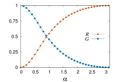
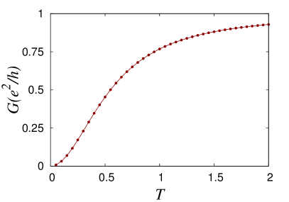
Figure 2: (Top) Reflection probability $\cal R$ (red circles) and different conductance $G=(e^{2}/h){\cal T}$ (blue squares) vs $\alpha$ of a wave packet which is centered at the site $L_{o}=50$ with width $\sigma=5$ on a lattice with $L=401$ sites. The kicking is done at the $L_{c}=201$-th site. The kicking time period is $T=0.5$, and the momentum is centered at $k_{c}=\pi/2$. The wave packet is evolved up to a time $(L-2L_{o})/|2\sin k_{c}|$. (Bottom) Differential conductance $G=(e^{2}/h){\cal T}$ vs $T$ when $\alpha=1$ is kept fixed. Other parameters are the same as in the top panel.

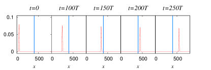
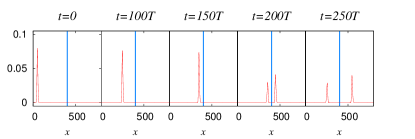
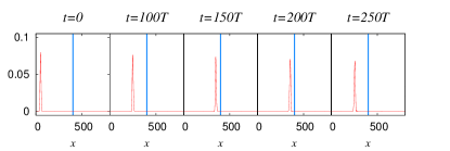
Figure 3: Transmission and reflection of a wave packet which is centered at the site $L_{o}=50$ with width $\sigma=5$ on a lattice with $L=801$ sites. The kicking is done at the $L_{c}=401$-th site (denoted by a vertical blue line). The kicking time period is $T=1$, and the momentum is centered at $k_{c}=\pi/2$. The wave packet is shown at various intervals of time. From top to bottom, the different cases correspond to kicking strengths $\alpha=0,~{}1.4$ and $3$. In the first case, the wave packet moves across the kicked site unhindered. In the second case, the original wave packet splits into two, one which transmits across the barrier and the other which reflects. In the third case, the wave packet gets completely reflects from the central site.

IV Perfect reflection and dynamical localization

A curious feature noted in the last section is that the wave packet completely reflects when the kicking strength $\alpha$ is close to $\pi$. This is intimately related to dynamical localization. We will make this connection clear in this section. It has been shown in previous work agarwala16 ; agarwala17 that a periodic kicks of strength $\pi$ on one sublattice of a bipartite system can lead to the phenomena of dynamical localization where a wave packet remains localized in space; this holds even when there is no disorder present in the system.

In the present context, the time evolution operator for a single time period $T$ can be written as

$$U~{}=~{}\exp(-i\alpha c^{\dagger}_{L_{c}}c_{L_{c}})~{}\exp[i\gamma T\sum_{n=1}^{L-1}(c^{\dagger}_{n}c_{n+1}+H.c.)].$$ (7)

It is particularly instructive to look at $U^{2}$ which evolves the system for a period $2T$. We rewrite $H_{TB}$ in Eq. htb as

$$H_{TB}~{}=~{}H_{r}~{}-~{}\gamma~{}(c^{\dagger}_{L_{c}}c_{L_{c}+1}+c^{\dagger}_{L_{c}}c_{L_{c}-1}+H.c.),$$ (8)

where $H_{r}$ denote the rest of the terms. Then

$$U^{2} = e^{-i\alpha c^{\dagger}_{L_{c}}c_{L_{c}}}~{}\exp(-iH_{TB}T)~{}\notag$$ (10)

$$\times~{}e^{-i\alpha c^{\dagger}_{L_{c}}c_{L_{c}}}~{}\exp(-iH_{TB}T).$$

We can evaluate this for $\alpha=\pi$ by noting that $e^{-i\pi c^{\dagger}_{L_{c}}c_{L_{c}}}=e^{i\pi c^{\dagger}_{L_{c}}c_{L_{c}}}$ (since $c^{\dagger}_{L_{c}}c_{L_{c}}$ can only take the values 0 and 1), and using the identities

$$e^{i\pi c^{\dagger}_{L_{c}}c_{L_{c}}}c_{L_{c}}e^{-i\pi c^{\dagger}_{L_{c}}c_{L_{c}}} = -~{}c_{L_{c}},$$

$$e^{i\pi c^{\dagger}_{L_{c}}c_{L_{c}}}c^{\dagger}_{L_{c}}e^{-i\pi c^{\dagger}_{L_{c}}c_{L_{c}}} = -~{}c^{\dagger}_{L_{c}}.$$ (11)

We then find

$$U^{2} = \exp[-iT\{H_{r}+\gamma(c^{\dagger}_{L_{c}}c_{L_{c}+1}+c^{\dagger}_{L_{c}}c_{L_{c}-1}+H.c.)\}]\notag$$ (12)

$$\times \exp[-iT\{H_{r}-\gamma(c^{\dagger}_{L_{c}}c_{L_{c}+1}+c^{\dagger}_{L_{c}}c_{L_{c}-1}+H.c.)\}].\notag$$ (13)

Using the Baker-Campbell-Hausdorff formula

$$e^{X}~{}e^{Y}~{}=~{}e^{X+Y+\frac{1}{2}[X,Y]+\cdots},$$ (15)

and assuming that $\gamma T\ll 1$, we can evaluate Eq. u2 to first order in $T$; we obtain

$$U^{2}~{}=~{}\exp(-i2H_{r}T).$$ (16)

We now examine the form of $H_{r}$. We see that $H_{r}$ is the part of the tight-binding Hamiltonian in which the hoppings to the central site are removed, i.e., $H_{r}$ is effectively described by two disconnected chains. This is the underlying reason why a wave packet completely reflects back at $\alpha=\pi$. Interestingly, this is also the regime which leads to dynamical localization in translationally invariant systems where the periodic kicking is applied to all the sites on one sublattice of a bipartite lattice agarwala16 ; agarwala17 .

We note here that the parameter $\alpha$ appearing in Eq. ut is really a periodic variable, namely, $\alpha$ and $\alpha+2\pi$ give the same results since $c^{\dagger}_{L_{c}}c_{L_{c}}$ can only take the values 0 and 1. In particular, $\alpha$ equal to any integer multiple of $2\pi$ will have no effect on the time evolution.

For later purposes, it is convenient to consider the Floquet eigenstates $\psi_{j}$ and eigenvalues $e^{-i\epsilon_{j}T}$ of the unitary operator $U$ defined in Eq. ut. The $\epsilon_{j}$’s are called quasienergies; since they are only defined modulo $2\pi/T$, we can take them to lie in the range $[-\pi/T,\pi/T]$.

V Non-Equilibrium Green’s function method

The non-equilibrium Green’s function (NEGF) method is one of the most robust methods for evaluating the conductance of a time-independent Hamiltonian datta . Here, we extend it to a periodically driven system and show that such a formalism appears to work for large driving frequencies or small time periods $T$.

The time evolution operator for a single time period $T$ can be written as

$$U = \exp(-i\alpha c^{\dagger}_{L_{c}}c_{L_{c}})~{}\exp[i\gamma T\sum_{n=1}^{L-1}(c^{\dagger}_{n}c_{n+1}+H.c.)]\notag$$ (17)

$$\equiv \exp(-iH_{eff}T),$$ (18)

where $H_{eff}$ can be found exactly by a numerical calculation. We now propose to use $H_{eff}$ as a time-independent Hamiltonian and implement the NEGF method. Namely, we use the Hamiltonian $H_{eff}$, along with the self-energies $\Sigma_{1}(E_{c})$ and $\Sigma_{2}(E_{c})$ at the left and right ends of the system (here $E_{c}=-2\gamma\cos k_{c}$ is the energy of a particle with momentum $k_{c}$), to compute the zero temperature differential conductance $G$ at the energy $E_{c}$. (See Ref. agarwal06, for details of the procedure).

The comparison of the differential conductance $G(E_{c})$ obtained using the NEGF method and the exact value using wave packet dynamics is shown in Fig. 4. (An analytical expression for $G(E_{c})$ will be presented in Eq. trans below for the case when $T$ is small). It is clear that the NEGF method using $H_{eff}$ works well for small $T$, but deviates significantly as $T$ becomes large. It is natural to ask what determines the crossover time scale between the two regimes. Another observation from Fig. 4 is that, even when $\alpha\sim\pi$, the wave packet dynamics shows that the transmission $\cal T$ is quite far from zero when the time period $T$ is large. Both of these observations can be understood by the following argument. Since a wave packet with width $\sigma$ and centered at a momentum $k_{c}$ has a velocity $|2\gamma\sin k_{c}|$, it will take a time $\Delta t=\sigma/|2\gamma\sin k_{c}|$ to cross any particular site on the lattice. If the kicking time period $T$ is larger than this $\Delta t$, one expects that the wave packet may not sample the kick and will therefore pass right through the site where the kicking is being applied. Therefore the kicking can properly affect the transmission only when

$$T~{}\lesssim~{}\frac{\sigma}{|2\gamma\sin k_{c}|}.$$ (19)

In Fig. 4, we have chosen $\sigma=5$ and $k_{c}=\pi/2$; this gives $T\lesssim 2.5$ in Eq. cond0. This explains why the NEGF results agree well with those based on wave packet dynamics if $T=0.4,~{}1.2$ and $2.4$, but not if $T=3.6$.

We note that the use of an effective Hamiltonian is only justified if $2\gamma T<\pi$; this can be seen as follows. We recall that the quasienergies $\epsilon_{j}$ are only defined up to multiples of the driving frequency $\omega=2\pi/T$. Since the $\epsilon_{j}$’s are eigenvalues of $H_{eff}$, this means that $H_{eff}$ is not uniquely defined to begin with. The eigenstates of $H_{TB}$ in Eq. htb lie in the range $[-2\gamma,2\gamma]$; hence if $2\gamma T<\pi$, we can define the quasienergies of all the bulk states to lie in the range $[-\pi/T,\pi/T]$. This will define $H_{eff}$ uniquely. On the other hand, the correspondence between the NEGF results and wave packet dynamics are expected to hold if the condition in Eq. cond0 holds; this condition depends on both the wave packet width $\sigma$ and the momentum $k_{c}$.

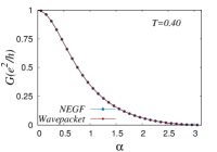
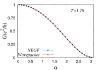
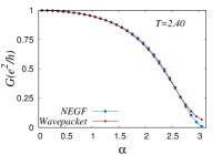
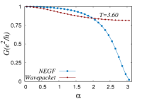
Figure 4: Differential conductance $G(E_{c})=(e^{2}/h){\cal T}(E_{c})$ vs $\alpha$. $G$ is computed from the dynamics of a wave packet which is centered at the site $L_{o}=50$ with width $\sigma=10$ on a lattice with $L=401$ sites. The kicking is done at the $201$-th site, and the time period takes the values $0.4,1.2,2.4$ and $3.6$ in the four figures from top left to bottom right. The momentum is centered at $k_{c}=\pi/2$, so that $E_{c}=0$. The transmissions obtained from the exact wave packet dynamics and the NEGF formalism are compared. We see that the NEGF formalism matches the exact results for small $T$.

VI Floquet bound states and resonances

In the presence of kicking we can study if there are Floquet bound states in the system and explore the properties of such bound states both analytically and using numerical techniques.

At high frequencies (i.e., small values of $T$), the effective Hamiltonian prescription, as briefly discussed in Sec. V, becomes more and more accurate. If both $\alpha$ and $\gamma T$ are small, we can use Eq. bch to show that the effective Hamiltonian is

$$H_{eff}~{}=~{}H_{TB}~{}+~{}\frac{\alpha}{T}c^{\dagger}_{L_{c}}c_{L_{c}}$$ (20)

to lowest order in $\alpha$ and $\gamma T$. This is effectively a time-independent system with a potential equal to $\alpha/T$ at the site $L_{c}$. It is known that such a potential on a lattice gives a transmission probability

$${\cal T}(k_{c})~{}=~{}\frac{4\gamma^{2}\sin^{2}k_{c}}{4\gamma^{2}\sin^{2}k_{c}~{}+~{}\frac{\alpha^{2}}{T^{2}}}$$ (21)

for a particle which is coming in with momentum $k_{c}$ and energy $E_{c}$. The form in Eq. trans explains the shape of the first plot in Fig. 4 where $T=0.4$ is small. A potential $\alpha/T$ at one site also produces a bound state with energy $\epsilon_{b}$ given by

$$\epsilon_{b}~{}=~{}\pm~{}\sqrt{4~{}+~{}\frac{\alpha^{2}}{T^{2}}},$$ (22)

where the sign of $\epsilon_{b}$ is the same as the sign of $\alpha/T$.

Numerically, given all the eigenstates of either a time-independent Hamiltonian $H$ or a time evolution operator $U$, the bound states can be identified quickly by looking at the values of the inverse participation ratio (IPR) of all the states. The IPR of a state $|\psi\rangle=\sum_{n=1}^{L}\psi(n)|n\rangle$ is defined as $\sum_{n=1}^{L}|\psi(n)|^{4}$. Typically, states which are spread over the entire system of length $L$ have an IPR of the order of $1/L$, while a bound state with a decay length $\lambda$ which is much smaller than $L$ will have an IPR of the order of $1/\lambda$ which is much larger than $1/L$. Hence a plot of the IPR versus the eigenstate number will clearly show the bound states manisha13 .

The bound state with the energy given in Eq. bounden has an exponentially decaying wave function of the form

$$\psi(n) = {\cal N}\exp(-|n-L_{c}|/\lambda)~{}~{}~{}{\rm if}~{}~{}~{}\frac{\alpha}{T}~{}<~{}0,$$

$$= {\cal N}~{}(-1)^{n}\exp(-|n-L_{c}|/\lambda)~{}~{}~{}{\rm if}~{}~{}~{}\frac{\alpha}{T}~{}>~{}0,$$

where the normalization constant ${\cal N}=\sqrt{\tanh(1/\lambda)}$, and the decay length $\lambda$ is given by

$$\lambda~{}=~{}\left({\rm arccosh}\sqrt{1+\frac{\alpha^{2}}{4T^{2}}}\right)^{-1}.$$ (24)

If $\lambda\gg 1$, one can show that the Fourier transform of the wave function in Eq. wavefn will have a peak at $k=0$ if $\alpha/T<0$ and at $k=\pm\pi$ if $\alpha/T>0$. (The Fourier transform of a wave function $\psi(n)$ is defined as ${\tilde{\psi}}(k)=\frac{1}{\sqrt{L}}\sum_{n=1}^{L}\psi(n)e^{-ikn}$). The IPR of the wave function in Eq. wavefn is given by

$${\rm IPR}~{}=~{}\frac{\alpha}{T}~{}\frac{\frac{\alpha^{2}}{T^{2}}+2}{\Big{(}\frac{\alpha^{2}}{T^{2}}+4\Big{)}^{3/2}}.$$ (25)

The highest IPR and its corresponding quasienergy calculated numerically for the eigenstates of the time evolution operator $U$ in Eq. heff and their comparison with the analytical expressions in Eqs. bounden and boundIPR is shown in Fig. 5. We will see later that the highest IPR corresponds to a bound state in certain regions of the “phase diagram” in the $\alpha-T$ plane but to a resonance in the continuum in other regions.

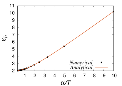
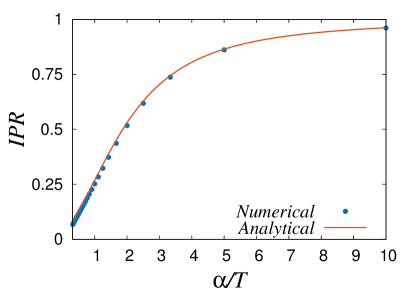
Figure 5: Bound state energy and IPR for $\alpha=0.5$ and different values of $T$. The numerically calculated spectrum matches well the analytical expression as shown in Eqs. bounden and boundIPR, for $L=401$ and $L_{c}=201$.

It is interesting to study the full phase diagram for this system. This is shown in the left panel of Fig. 6 when there is no time-independent on-site potential (i.e., $V=0$, where $V$ is defined in Eq. hv). With increasing $\alpha$ one finds that the IPR increases, while increasing $T$ reduces IPR. Both of these are expected results since the effective potential due to the kicking is given by $\alpha/T$. However we find that the bound state appears to vanish abruptly when $T$ increases beyond $\pi/2$. This value of $T$ corresponds to the driving frequency $\omega=4$ which is also the band width of the tight-binding model with $\gamma=1$. Since the quasienergies of the bulk states (namely, the states which are extended throughout the system) form a continuum going from $-2\gamma$ to $2\gamma$. Hence, for $T<\pi/2$, the quasienergies do not cover the full range $[-\pi/T,\pi/T]$; this makes it possible for a bound state to appear with a quasienergy which does not lie in the range of the bulk quasienergies; hence the bound and bulk states do not mix. However, for $T>\pi/2$, the bulk quasienergies cover the full range; hence any bound states must have a quasienergy which lies in the continuum of the bulk quasienergies. Such a situation is generally not possible except in special cases where the bound and bulk states cannot mix due to some symmetry or topological reasons; see Ref. bic, and references therein. Thus the disappearance of bound states above a certain value of $T$ is a unique feature of the Floquet system, since in a time-independent system in one dimension, a non-zero potential will always produce a bound state. Although there are no bound states for $T>\pi/2$, we will now see that there can be a resonance in the continuum; such a state is a superposition of a state which is localized near one point and some of the bulk states.

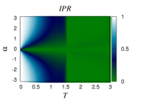
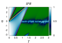
Figure 6: The maximum IPR value of the eigenstates of the time evolution operator as a function of $T$ and $\alpha$ for $V=0$ (left panel) and $V=-4$ (right panel). The system has $L=401$ sites and the central site is kicked periodically. For $V=0$, the IPR increases as $\alpha$ increases, while increasing $T$ reduces the IPR. When $T$ crosses $\pi/2$ the bound state (which has the largest IPR) ceases to exist.

In Fig. 7, we show the Floquet eigenvalues (since the time evolution operator is unitary, its eigenvalues lie on a unit circle in the complex plane), the probabilities $|\psi(n)|^{2}$ at different sites of a bound state, and the square of the modulus of the Fourier transform of the bound state for a system with 401 sites in which periodic $\delta$-function kicks are applied at the $201$-th site with strength $\alpha=0.4$ and time period $T=1$. The bound state is easily identified because it has the largest IPR equal to $0.0936$. Its Floquet eigenvalue is equal to $-0.4473-0.8944i$ which is shown by a large red dot lying just outside the continuum of the eigenvalues of the bulk states; this eigenvalue agrees well with $\exp(-i\epsilon_{b}T)=-0.4518-0.8921i$, where $\epsilon_{b}=\sqrt{4+\alpha^{2}/T^{2}}$ is the bound state energy given in Eq. bounden. According to Eq. decay, the decay length of this state is equal to $\lambda=5$. The IPR equal to $0.0936$ agrees fairly well with the value of $0.1018$ given by Eq. boundIPR. The square of the modulus of the Fourier transform, $|{\tilde{\psi}}(k)|^{2}$, of the bound state is found to have peaks at $k=\pm\pi$.

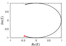
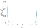
Figure 7: (Left) Eigenvalues of time evolution operator for a system with 401 sites in which $\delta$-function kicks are applied at the $201$-th site with $\alpha=0.4$ and $T=1$. There is a bound state with IPR equal to $0.0936$ and Floquet eigenvalue equal to $-0.4473-0.8944i$ shown by a large red dot. (Middle) Probability $|\psi(n)|^{2}$ of the bound state. (Right) Square of the modulus of the Fourier transform, $|{\tilde{\psi}}(k)|^{2}$, of the bound state. It has peaks at $k=\pm\pi$.

Figure 8 shows the Floquet eigenvalues, the probabilities $|\psi(n)|^{2}$ at different sites of a resonance state, and the square of the modulus of the Fourier transform of the resonance state for a system with 401 sites in which $\delta$-function kicks are applied at the $201$-th site with $\alpha=0.4$ and $T=2$. The resonance state has the largest IPR equal to $0.0324$. Its Floquet eigenvalue is equal to $-0.6388+0.7694i$ which is shown by a large red dot lying within the continuum of the bulk eigenvalues; this value again agrees well with $\exp(-i\epsilon_{b}T)=-0.6384+0.7697i$, where $\epsilon_{b}$ is the bound state energy given in Eq. bounden (the bound state has turned into a resonance here due to mixing with the bulk states). According to Eq. decay, the decay length of this state is equal to $\lambda=10$. The IPR equal to $0.0324$ is significantly smaller than the value of $0.0502$ given by Eq. boundIPR; this is because of a substantial mixing with plane waves with $k=\pm 0.967$ (found from the peaks in the Fourier transform). According to Eq. decay, the decay length of this state is equal to $\lambda=10$. The square of the modulus of the Fourier transform, $|{\tilde{\psi}}(k)|^{2}$, of the bound state is found to have peaks at both $k=\pm\pi$ and $k=\pm 0.967$. We can understand the peaks at $k=\pm 0.967$ as follows: we note that there are bulk states at these values of $k$ with a Floquet eigenvalue equal to $\exp(i2\gamma T\cos k)=-0.6444+0.7647i$. This is close to the Floquet eigenvalue of the resonance state which can therefore mix easily with these bulk states.

To see how the IPR of a bound or resonance state varies with the system size, we study the maximum IPR versus $L$, taking $L$ to be odd, the kicking site to be at the middle, $L_{c}=(L+1)/2$, and open boundary conditions. For $\alpha=0.4$ and $T=1$, we find that the maximum IPR is equal to $0.0936$ and is independent of the system size in the range $101\leq L\leq 799$. (We have chosen this range so that $L$ is much larger than the decay length $\lambda$ of the central part of the state). This size independence is a signature of a bound state. On the other hand, for $\alpha=0.4$ and $T=2$, we find that the maximum IPR fluctuates significantly for small changes in $L$ but on the average decreases as $L$ increases. This is shown in Fig. 9; the fluctuations demonstrate a sensitivity to the system size and confirm that it is a resonance rather than a bound state. We have chosen a fit of the form $IPR=a/L^{b}$; we find that the best fit is given by the exponent $b=0.41$ for $\alpha=0.4,~{}T=2$, and $0.83$ for $\alpha=1,~{}T=2.5$. This is to be compared with the IPRs of the bulk states which decrease as $1/L$. Thus although the peak value of the wave function goes to zero as $L$ increases, the ratio of the peak value to the value of the wave function far from the peak grows with $L$. The value of the exponent $b$ is not universal; we find that it depends on the values of $\alpha$ and $T$. However, it is smaller than 1 over a wide range of parameters and reasonably large system sizes, implying that although the IPR of the resonance state decreases, the IPRs of the bulk states decrease even faster as $L$ increases.

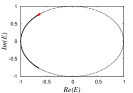
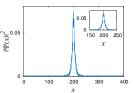
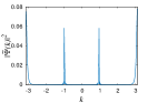
Figure 8: (Left) Eigenvalues of time evolution operator for a system with 401 sites in which $\delta$-function kicks are applied to the $201$-th site with strength $\alpha=0.4$ and time period $T=2$. (There are more eigenvalues on the left side than on the right side; hence the plot looks solid on the left and dotted on the right). There is a resonance state with Floquet eigenvalue equal to $-0.6388+0.7694i$ shown by a large red dot. (Middle) Probability $|\psi(n)|^{2}$ of the resonance state. (Right) Square of the modulus of the Fourier transform, $|{\tilde{\psi}}(k)|^{2}$, of the resonance state. It has peaks at both $k=\pm\pi$ and $k=\pm 0.967$, thus showing a substantial mixing with the bulk states.

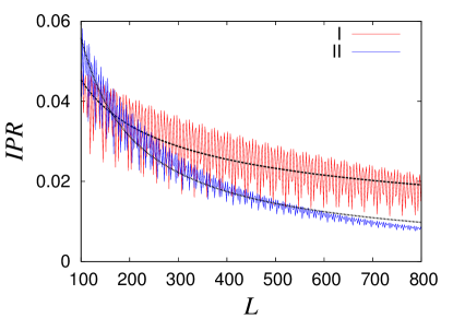
Figure 9: The maximum IPR value of the eigenstates of the time evolution operator as a function of the system size $L$ for (I) $\alpha=0.4$ and $T=2$ and (II) $\alpha=1.0$ and $T=2.5$. Curve I corresponding to the lower value of $\alpha$ has much larger fluctuations than curve II. The dotted lines show a fit of the form $IPR=a/L^{b}$ for the average IPR; for (I) the values $a=0.31$ and $b=0.41$ give the best fit; for (II) $a=2.65$ and $b=0.83$.

To summarize, we find that a bound state differs from a resonance in several ways.

(i) The Floquet eigenvalue of a bound state lies outside the continuum of the Floquet eigenvalues of the bulk states, while the Floquet eigenvalue of a resonance lies within the continuum of the bulk eigenvalues.

(ii) The wave function of a bound state is peaked at some point, decays rapidly away from that point, and essentially becomes zero beyond some distance. The wave function of a resonance is also peaked at some point and decays away from that point, but it does not become completely zero no matter how far we go; this is because it contains a non-zero superposition of some plane waves and therefore remains non-zero even far away from the peak.

(iii) If the system size is large enough, the properties of a bound state, such as its IPR and the peak value of its wave function, become independent of the system size $L$ and the boundary conditions (for instance, whether we have periodic, anti-periodic or open boundary conditions). For a resonance, however, the IPR and peak value of the wave function depend sensitively on the boundary conditions and the value of $L$, and on the average they keep decreasing as $L$ is increased. This is because such a state contains some plane waves which sample the entire system, and the quasienergies of the plane waves is sensitively dependent on the boundary conditions and $L$. (We recall that if periodic boundary conditions are imposed, the momentum of the plane wave states is quantized in units of $2\pi/L$. Hence the values of the momentum and therefore the quasienergies $-2\gamma\cos k$ depend on $L$).

Next, we introduce a time-independent on-site potential at the same site where the periodic kicking is being applied; this potential is given by

$$H_{V}=Vc^{\dagger}_{L_{c}}c_{L_{c}}.$$ (26)

To investigate the effects of kicking, we again plot the maximum value of the IPR of all the eigenstates of the time evolution operator as a function of $T$ and $\alpha$. This is shown in the right panel of Fig. 6 for $V=-4$. We see a number of features in this plot including some straight lines; we now provide a qualitative understanding of these features. The bold lines within which the IPR is close to 1 is basically determined by whether the bound state mixes with the continuum states or not. Since the bulk quasienergies lie between $-2\gamma$ and $2\gamma$, the bound state does not mix with the continuum states and therefore exists in the regions

$$\epsilon_{b}~{}+~{}\frac{\alpha}{T} > 2\gamma,$$ (27)

$$\epsilon_{b}~{}+~{}\frac{\alpha}{T} < -2\gamma,$$ (28)

where $\epsilon_{b}$ is the bound state energy

$$\epsilon_{b}~{}=~{}-\sqrt{V^{2}+4\gamma^{2}}$$ (29)

produced by an on-site potential $V<0$. Similar to the condition in Eq. cond1 and using the fact that quasienergies are only defined modulo $2\pi/T$, we see that another line for the existence of a bound state is given by

$$\epsilon_{b}~{}+~{}\frac{\alpha}{T}~{}>~{}-~{}\frac{2\pi}{T}~{}+~{}2\gamma.$$ (30)

Between the two lines given in Eqs. cond1 and cond2 and below the line given in Eq. cond3, the bound state mixes with the bulk quasienergies and therefore turns into a resonance in the continuum.

VII Increase in conductance due to periodic kicking

In the presence of only a time-independent on-site potential $V$, we have a bound state and a transmission probability $\cal T$ which is less than 1. We now ask if the transmission can be increased by periodic kicking at the same site where the potential $V$ is present. In Sec. II we saw that the transmission can get reduced when we introduce kicking. We now look at the opposite case where periodic driving can increase the transmission. In Fig. 10. the differential conductance is shown as a function of $\alpha$ for a system with $T=0.5$, $V=-4$ and $k_{c}=\pi/2$. The maximum transmission should occur at $\alpha=-VT$ which is equal to $2$ for the parameters used in Fig. 10. We see in that figure that this is indeed true and the system becomes “transparent” when $\alpha=-VT$.

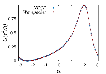
Figure 10: Differential conductance $G=(e^{2}/h){\cal T}$ vs $\alpha$ for a system with $V=-4$. We see that $\alpha$ can tune the conductance all the way from zero to 1. Here $L=401$, $k_{c}=\pi/2$, $L_{o}=50$, $\sigma=5$, and $T=0.5$.

VIII Effects of Interactions

We now analyze the effects of interactions on the various aspects that we have discussed so far, namely, transport and the presence of bound states. We consider a system containing two species of electrons with up and down spins and a time-independent interacting term on the site $L_{c}$. The total Hamiltonian is

$$H = -~{}\gamma~{}\sum_{n=1}^{L-1}~{}\sum_{\sigma=\uparrow,\downarrow}~{}(c^{\dagger}_{n\sigma}c_{n+1,\sigma}+H.c.)\notag$$ (33)

$$+~{}\alpha~{}\sum_{m=-\infty}^{\infty}~{}\delta(t-mT)~{}c^{\dagger}_{L_{c}\sigma}c_{L_{c}\sigma}\notag$$

$$+~{}U~{}\hat{n}_{L_{c}\uparrow}\hat{n}_{L_{c}\downarrow},$$

where $\hat{n}_{L_{c}\sigma}$ is the number operator for electrons with spin $\sigma$ at site $L_{c}$. In order to investigate the effect of the interaction term, we begin with an initial wave packet which has two-particles in a singlet state of $\psi_{\uparrow}(r)$ and $\psi_{\downarrow}(r)$; the form of the wave packet is given in Eq. eqn:wavepa. We then study the effects of the interaction using exact diagonalization and wave packet evolution. The effect of $U$ is shown in Fig. 11 where the reflection probability for an electron with spin-up, ${\cal R}_{\uparrow}$, is shown as a function of $U$. [Given an amplitude $\psi(n_{1},n_{2})$ for a spin-up electron to be at $n_{1}$ and a spin-down electron to be at $n_{2}$, we define the reflection and transmission probabilities for a spin-up electron to be ${\cal R}_{\uparrow}=\sum_{n_{1}=1}^{L_{c}}\sum_{n_{2}=1}^{L}|\psi(n_{1},n_{2})|^{2}$ and ${\cal T}_{\uparrow}=\sum_{n_{1}=L_{c}+1}^{L}\sum_{n_{2}=1}^{L}|\psi(n_{1},n_{2})|^{2}$, analogous to Eq. rt. These satisfy ${\cal R}_{\uparrow}+{\cal T}_{\uparrow}=1$. We can similarly define ${\cal R}_{\downarrow}$ and ${\cal T}_{\downarrow}$; our choice of the form of the wave packet implies that ${\cal R}_{\uparrow}={\cal R}_{\downarrow}$ and ${\cal T}_{\uparrow}={\cal T}_{\downarrow}$]. Increasing $\alpha$ makes $U$ less effective; this is because in the presence of kicking, the wave packet is small at the site $L_{c}$ and is therefore unable to sample the interaction. Note that in the presence of $\alpha$, the effects of $U$ and $-U$ are different. This is because the driving produces an effective on-site potential equal to $\alpha/T$; hence the total quasienergy of a state with two electrons at site $L_{c}$ is $U+2\alpha/T$. The minimum of this energy (and hence the minimum of the reflection probability) occurs at a non-zero value of $U$.

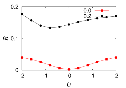
Figure 11: Reflection probability ${\cal R}_{\uparrow}$ of a spin-up electron for a wave packet in a system with an on-site interaction $U$ and kicking strengths $\alpha=0$ (lower curve) and $0.2$ (upper curve). Even with $\alpha=0$ the wave packet is not completely transmitted in the presence of a finite $U$. This happens because there is a finite probability for the incoming wave packet to get trapped in a bound state which lives near the interacting site. The effect of $U$ acts asymmetrically in the presence of a finite $\alpha$. The effect of $U$ reduces with increasing $\alpha$ and at large values of $\alpha$, ${\cal R}_{\uparrow}$ is independent of $U$. We have taken $L=51$, $T=0.25$, $k_{c}=\pi/2$, $\sigma=4$, and $L_{o}=6$.

As in the case of a non-interacting system, we find that Floquet bound states can also appear in the presence of interactions. They have an interesting dependence on the time period $T$. If $U\gg\gamma$, there will be a bound state in which both electrons are at the site $L_{c}$, and the quasienergy of this state is $U+2\alpha/T$ in the presence of kicking. Since the energy of the bulk states of the two-electron system goes $-4\gamma$ to $4\gamma$, the bound state will not mix with the bulk states if

$$U~{}+~{}\frac{2\alpha}{T} > 4\gamma,$$ (34)

$$U~{}+~{}\frac{2\alpha}{T} < -4\gamma.$$ (35)

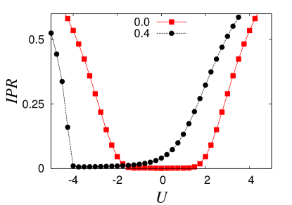
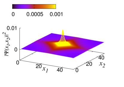
Figure 12: (Top) The value of the two-body IPR for the state with the maximum IPR as a function of the Hubbard interaction $U$, with and without periodic driving. We have taken $L=51$, $T=0.5$, $\alpha=0.4$ (black disks) and $\alpha=0$ (red squares). (Bottom) A two-particle bound state wave function for $L=51$, $T=0.5$, $\alpha=0.4$, and $U=1$ where a much more localized bound state is produced by the driving.

We can calculate the IPR of a two-particle state and study its variation with $U$; this is shown in Fig. 12. In the absence of kicking ($\alpha=0$), we find that for $|U|\lesssim 2$, the IPR is not very high suggesting a state which is not strongly localized, while for $|U|\gtrsim 2$, the IPR is large which suggests a strongly localized state. Interestingly, we find that a finite kicking strength (such as $\alpha=0.4$) can turn a strongly localized state into a weakly localized one and vice versa, depending on the values of $U$ and $T$. A strongly localized two-particle bound state wave function is shown in Fig. 12.

IX Conclusions

In this paper we have studied the effects of periodic driving at one site in some tight-binding lattice models in one dimension. We have taken the driving to be of the form of periodic $\delta$-function kicks with strength $\alpha$ and time period $T$. We have studied how the kicking affects transmission across that site and whether it produces any bound states.

The transmission (which is related to the differential conductance) has been calculated by constructing an incoming wave packet which is centered around a particular momentum and time evolving it numerically. The reflection and transmission probabilities are found by computing the total probabilities on the left and right sides of the kicking site after a sufficiently long time. The bound state is found by computing all the eigenstates of the time evolution operator $U$ for one time period, and finding the eigenstate with the maximum value of the inverse participation ratio; we look at the corresponding wave function to confirm that it is indeed peaked near the kicking site.

When $T$ is much smaller than the inverse of the hopping $\gamma$ and $|\alpha|\ll 1$, the numerically obtained values of both the transmission probability and the Floquet quasienergy of the bound state are consistent with the fact that the kicking effectively acts like a time-independent potential equal to $\alpha/T$ at the special site. This is confirmed by calculating the effective Hamiltonian and then using the non-equilibrium Green’s function method to compute the transmission; this is found to agree well with the transmission found from wave packet dynamics if $T$ is small. When $T$ is small and $\alpha=\pi$, we find that the transmission probability is zero; this is because the effective hoppings between the kicked site and its two neighboring sites become zero, and it is related to the phenomenon of dynamical localization. On the other hand, when $T$ becomes comparable to $1/\gamma$, the agreement between the transmissions found using wave packet dynamics and the effective Hamiltonian breaks down, showing that the effective Hamiltonian no longer provides an accurate description of the system.

We note that the effective breaking of a “bond” in the Floquet description is a unique result and cannot be found in a static case. This feature is true even in higher dimensions and therefore provides a unique opportunity to experimentally simulate bond percolation problems Sen09 in cold atom or photonic systems. In such systems local $\delta$-function kicking can be implemented at randomly chosen sites in the system and their effect on the localization physics can be investigated.

A bound state can appear only if its quasienergy does not lie the continuum of the quasienergies of the bulk states going from $-2\gamma$ to $2\gamma$ modulo $2\pi/T$. If the Floquet quasienergy of the would-be bound state lies within the continuum of the quasienergies of the bulk states (this necessarily happens if $T>\pi/(2\gamma)$ but it can also happen for certain values of $\alpha$ if $T<\pi/(2\gamma)$), the bound state ceases to exist. However, we then find that in certain ranges of values of $\alpha$ and $T$, there is a state which can be described as a resonance in the continuum. The wave function of such a state consists of a superposition of a strongly peaked part which resembles a bound state and a plane wave part which does not decay even far away from the kicking site. Further, the IPR of this state is sensitively dependent on the system size and boundary conditions and it gradually decays as the system size is increased. This behavior is in contrast to a bound state whose IPR becomes independent of the system size and boundary conditions when the system size is larger than the decay length.

Next, we have studied what happens if there is a time-independent potential $V$ at a single site and periodic $\delta$-function kicks are applied to the same site. Separately both $V$ and the kicks reduce the transmission from unity and can produce bound states. When both of them are present, we get a complex pattern of regions in the $\alpha-T$ plane where bound states are present. These regions can be understood using a simple condition that the sum of the effective on-site potential $\alpha/T$ due to the kicking and the energy of the bound state produced by $V$ alone should not lie within the continuum of the quasienergies of the bulk states. Further, if $V$ and $\alpha/T$ have opposite signs, their effects can partially cancel each other and the transmission probability can be higher than if only one of them was present.

Finally, we have studied a model with spin-1/2 electrons where there is a Hubbard interaction of strength $U$ at a single site and periodic kicks are applied to the same site. We numerically study wave packet dynamics starting with an initial wave packet which contains two electrons in a spin singlet state. In the absence of kicking, a state in which both particles are at the special site has an energy $U$. This has a similar effect as an on-site potential for the model of spinless electrons; the transmission probability is therefore reduced from 1 for any non-zero value of $U$, and it has the same value for $U$ and $-U$. When we introduce kicking, the effective potential for two particles at the special site is given by the sum of $U$ and $2\alpha/T$. Hence the transmission probability will be higher when $U$ and $2\alpha/T$ have opposite signs, and will therefore not be symmetric under $U\to-U$. We also find that a bound state can appear if its quasienergy does not lie within the continuum of bulk quasienergies. When $U$ is non-zero, we find that kicking can convert strongly localized states to weakly localized ones and vice versa.

We end by pointing out some directions for future studies.

(i) In this paper we have only examined systems with one or two particles. It may be interesting to study a thermodynamic system with a finite filling fraction of particles. One can then investigate if, for example, the model of spin-1/2 electrons with both an interaction $U$ and periodic kicking at the same site can show a Kondo-like resonance hewson97 ; kaminski00 . Related problems have been studied in Refs. heyl10, ; iwahori16, .

(ii) It may be interesting to look at the effects of heating. It is known that a system generally heats up to infinite temperature when there are interactions and periodic driving at all the sites bilitewski15 ; genske15 ; kuwahara16 . However, if interactions and periodic driving are both present in only a small region as considered in this paper, it is not known if the system will heat up indefinitely at long times.

(iii) The effects of periodic kicking at more than one site, possibly with different strengths and phases, would be interesting to study. It is known that harmonic driving at two sites with a phase difference can pump charge (see Ref. soori10, for references). We therefore expect that the application of $\delta$-function kicks at two sites may also pump charge. In addition, we can study what kinds of bound states are generated in such a system.

There has been an increasing interest in understanding the dynamics of a single impurity or of electrons in a quantum dot under the periodic modulation of some parameter. This is motivated both by theoretical considerations such as the effect of such a modulation on the Kondo effect iwahori16 ; Suzuki17 and by advances in cold atom experiments which allow for the imaging and modulation of systems up to single site resolution Fukuhara13 ; Fukuhara132 ; Hild14 . The results presented in this manuscript describe many interesting phenomena which are realizable due to an interplay of impurity physics and dynamical modulation of some parameter in the Hamiltonian. It will be interesting if such effects can indeed be observed in cold atom or mesoscopic systems.

References

- (1)
- (2) F. Grossmann, T. Dittrich, P. Jung, and P. Hänggi, Phys. Rev. Lett. 67, 516 (1991).
- (3) Y. Kayanuma, Phys. Rev. A 50, 843 (1994).
- (4) V. Mukherjee, A. Dutta, and D. Sen, Phys. Rev. B 77, 214427 (2008); V. Mukherjee and A. Dutta, J. Stat. Mech. (2009) P05005.
- (5) A. Das, Phys. Rev. B 82, 172402 (2010); S. S. Hegde, H. Katiyar, T. S. Mahesh, and A. Das, Phys. Rev. B 90, 174407 (2014).
- (6) A. Russomanno, A. Silva, and G. E. Santoro, Phys. Rev. Lett. 109, 257201 (2012).
- (7) L. D’Alessio and A. Polkovnikov, Annals of Physics 333, 19 (2013); M. Bukov, L. D’Alessio, and A. Polkovnikov, Advances in Physics 64, 139 (2015).
- (8) T. Nag, S. Roy, A. Dutta, and D. Sen, Phys. Rev. B 89, 165425 (2014); T. Nag, D. Sen, and A. Dutta, Phys. Rev. A 91, 063607 (2015).
- (9) A. Agarwala, U. Bhattacharya, A. Dutta, and D. Sen, Phys. Rev. B 93, 174301 (2016).
- (10) S. Sharma, A. Russomanno, G. E. Santoro, and A. Dutta, EPL 106, 67003 (2014).
- (11) A. Russomanno, S. Sharma, A. Dutta, and G. E. Santoro, J. Stat. Mech. (2015) P08030.
- (12) A. Lazarides, A. Das, and R. Moessner, Phys. Rev. Lett. 112, 150401 (2014).
- (13) A. Dutta, G. Aeppli, B. K. Chakrabarti, U. Divakaran, T. Rosenbaum and D. Sen, Quantum Phase Transitions in Transverse Field Spin Models: From Statistical Physics to Quantum Information (Cambridge University Press, Cambridge, 2015).
- (14) Z. Gu, H. A. Fertig, D. P. Arovas, and A. Auerbach, Phys. Rev. Lett. 107, 216601 (2011).
- (15) T. Kitagawa, T. Oka, A. Brataas, L. Fu, and E. Demler, Phys. Rev. B 84, 235108 (2011).
- (16) E. Suárez Morell and L. E. F. Foa Torres, Phys. Rev. B 86, 125449 (2012).
- (17) M. A. Sentef, M. Claassen, A. F. Kemper, B. Moritz, T. Oka, J. K. Freericks, and T. P. Devereaux, Nature Commun. 6, 7047 (2015).
- (18) T. Kitagawa, E. Berg, M. Rudner, and E. Demler, Phys. Rev. B 82, 235114 (2010).
- (19) N. H. Lindner, G. Refael, and V. Galitski, Nature Phys. 7, 490 (2011).
- (20) L. Jiang, T. Kitagawa, J. Alicea, A. R. Akhmerov, D. Pekker, G. Refael, J. I. Cirac, E. Demler, M. D. Lukin, and P. Zoller, Phys. Rev. Lett. 106, 220402 (2011).
- (21) M. Trif and Y. Tserkovnyak, Phys. Rev. Lett. 109, 257002 (2012).
- (22) A. Gomez-Leon and G. Platero, Phys. Rev. B 86, 115318 (2012), and Phys. Rev. Lett. 110, 200403 (2013).
- (23) B. Dóra, J. Cayssol, F. Simon, and R. Moessner, Phys. Rev. Lett. 108, 056602 (2012); J. Cayssol, B. Dora, F. Simon, and R. Moessner, Phys. Status Solidi RRL 7, 101 (2013).
- (24) D. E. Liu, A. Levchenko, and H. U. Baranger, Phys. Rev. Lett. 111, 047002 (2013).
- (25) Q.-J. Tong, J.-H. An, J. Gong, H.-G. Luo, and C. H. Oh, Phys. Rev. B 87, 201109(R) (2013).
- (26) M. S. Rudner, N. H. Lindner, E. Berg, and M. Levin, Phys. Rev. X 3, 031005 (2013).
- (27) Y. T. Katan and D. Podolsky, Phys. Rev. Lett. 110, 016802 (2013).
- (28) N. H. Lindner, D. L. Bergman, G. Refael, and V. Galitski, Phys. Rev. B 87, 235131 (2013).
- (29) A. Kundu and B. Seradjeh, Phys. Rev. Lett. 111, 136402 (2013).
- (30) V. M. Bastidas, C. Emary, G. Schaller, A. Gómez-León, G. Platero, and T. Brandes, arXiv:1302.0781.
- (31) T. L. Schmidt, A. Nunnenkamp, and C. Bruder, New J. Phys. 15, 025043 (2013).
- (32) A. A. Reynoso and D. Frustaglia, Phys. Rev. B 87, 115420 (2013).
- (33) C.-C. Wu, J. Sun, F.-J. Huang, Y.-D. Li, and W.-M. Liu, EPL 104, 27004 (2013).
- (34) M. Thakurathi, A. A. Patel, D. Sen, and A. Dutta, Phys. Rev. B 88, 155133 (2013).
- (35) P. M. Perez-Piskunow, G. Usaj, C. A. Balseiro, and L. E. F. Foa Torres, Phys. Rev. B 89, 121401(R) (2014); G. Usaj, P. M. Perez-Piskunow, L. E. F. Foa Torres, and C. A. Balseiro, Phys. Rev. B 90, 115423 (2014); P. M. Perez-Piskunow, L. E. F. Foa Torres, and G. Usaj, Phys. Rev. A 91, 043625 (2015).
- (36) M. D. Reichl and E. J. Mueller, Phys. Rev. A 89, 063628 (2014).
- (37) M. Thakurathi, K. Sengupta, and D. Sen, Phys. Rev. B 89, 235434 (2014).
- (38) M. Claassen, C. Jia, B. Moritz, and T. P. Devereaux, Nature Commun. 7, 13074 (2016).
- (39) S. Saha, S. N. Sivarajan, and D. Sen, Phys. Rev. B 95, 174306 (2017).
- (40) H. Hübener, M. A. Sentef, U. De Giovannini, A. F. Kemper, and A. Rubio, Nature Commun. 8, 13940 (2017).
- (41) T. Kitagawa, M. A. Broome, A. Fedrizzi, M. S. Rudner, E. Berg, I. Kassal, A. Aspuru-Guzik, E. Demler, and A. G. White, Nature Commun. 3, 882 (2012).
- (42) M. C. Rechtsman, J. M. Zeuner, Y. Plotnik, Y. Lumer, D. Podolsky, S. Nolte, F. Dreisow, M. Segev, and A. Szameit, Nature (London) 496, 196 (2013); M. C. Rechtsman, Y. Plotnik, J. M. Zeuner, D. Song, Z. Chen, A. Szameit, and M. Segev, Phys. Rev. Lett. 111, 103901 (2013); Y. Plotnik, M. C. Rechtsman, D. Song, M. Heinrich, J. M. Zeuner, S. Nolte, Y. Lumer, N. Malkova, J. Xu, A. Szameit, Z. Chen, and M. Segev, Nature Materials 13, 57 (2014).
- (43) L. Tarruell, D. Greif, T. Uehlinger, G. Jotzu, and T. Esslinger, Nature (London) 483, 302 (2012).
- (44) G. Jotzu, M. Messer, R. Desbuquois, M. Lebrat, T. Uehlinger, D. Greif, and T. Esslinger, Nature (London) 515, 237 (2014).
- (45) A. Eckardt, C. Weiss, and M. Holthaus, Phys. Rev. Lett. 95, 260404 (2005).
- (46) A. Rapp, X. Deng, and L. Santos, Phys. Rev. Lett. 109, 203005 (2012).
- (47) W. Zheng, B. Liu, J. Miao, C. Chin, and H. Zhai, Phys. Rev. Lett. 113, 155303 (2014).
- (48) S. Greschner, L. Santos, and D. Poletti, Phys. Rev. Lett. 113, 183002 (2014).
- (49) A. Lazarides, A. Das, and R. Moessner, Phys. Rev. E 90, 012110 (2014); A. Lazarides, A. Das, and R. Moessner, Phys. Rev. Lett. 115, 030402 (2015).
- (50) L. D’Alessio and M. Rigol, Phys. Rev. X 4, 041048 (2014).
- (51) P. Ponte, Z. Papić, F. Huveneers, and D. A. Abanin, Phys. Rev. Lett. 114, 140401 (2015); P. Ponte, A. Chandran, Z. Papić, and D. A. Abanin, Annals of Physics 353, 196 (2015).
- (52) A. Eckardt and E. Anisimovas, New J. Phys. 17, 093039 (2015).
- (53) M. Bukov, M. Kolodrubetz, and A. Polkovnikov, Phys. Rev. Lett. 116, 125301 (2016).
- (54) V. Khemani, A. Lazarides, R. Moessner, and S. L. Sondhi, Phys. Rev. Lett. 116, 250401 (2016).
- (55) C. W. von Keyserlingk, V. Khemani, and S. L. Sondhi, Phys. Rev. B 94, 085112 (2016).
- (56) D. V. Else, B. Bauer, and C. Nayak, Phys. Rev. Lett. 117, 090402 (2016); D. V. Else, B. Bauer, and C. Nayak, Phys. Rev. X 7, 011026 (2017).
- (57) A. P. Itin and M. I. Katsnelson, Phys. Rev. Lett. 115, 075301 (2015).
- (58) T. Mikami, S. Kitamura, K. Yasuda, N. Tsuji, T. Oka, and H. Aoki, Phys. Rev. B 93, 144307 (2016).
- (59) J. Klinovaja, P. Stano, and D. Loss, Phys. Rev. Lett. 116, 176401 (2016).
- (60) M. Thakurathi, D. Loss, and J. Klinovaja, Phys. Rev. B 95, 155407 (2017).
- (61) W. Su, M. N. Chen, L. B. Shao, L. Sheng, and D. Y. Xing, Phys. Rev. B 94, 075145 (2016).
- (62) M. Račiūnas, G. Žlabys, A. Eckardt, and E. Anisimovas, Phys. Rev. A 93, 043618 (2016).
- (63) F. Meinert, M. J. Mark, K. Lauber, A. J. Daley, and H.-C. Nägerl, Phys. Rev. Lett. 116, 205301 (2016).
- (64) P. Bordia, H. P. Lüschen, S. S. Hodgman, M. Schreiber, I. Bloch, and U. Schneider, Phys. Rev. Lett. 116, 140401 (2016); P. Bordia, H. Lüschen, U. Schneider, M. Knap, and I. Bloch, Nature Phys. 13, 460 (2017).
- (65) S. Mukherjee, M. Valiente, N. Goldman, A. Spracklen, E. Andersson, P. Öhberg, and R. R. Thomson, Phys. Rev. A 94, 053853 (2016).
- (66) B. V. Chirikov, F. M. Izrailev, and D. L. Shepelyansky, Sov. Sci. Rev. C 2, 209 (1981).
- (67) S. Fishman, D. R. Grempel, and R. E. Prange, Phys. Rev. Lett. 49, 509 (1982).
- (68) H. Ammann, R. Gray, I. Shvarchuck, and N. Christensen, Phys. Rev. Lett. 80, 4111 (1998).
- (69) C. Tian, A. Altland, and M. Garst, Phys. Rev. Lett. 107, 074101 (2011).
- (70) E. P. L. van Nieuwenburg, J. M. Edge, J. P. Dahlhaus, J. Tworzydlo, and C. W. J. Beenakker, Phys. Rev. B 85, 165131 (2012).
- (71) P. L. Kapitza, Sov. Phys. JETP 21, 588 (1951).
- (72) H. W. Broer, I. Hoveijn, M. van Noort, C. Simon, and G. Vegter, Journal of Dynamics and Differential Equations, 16 897 (2004).
- (73) B. Horstmann, J. I. Cirac, and T. Roscilde, Phys. Rev. A. 76, 043625 (2007).
- (74) A. Roy and A. Das, Phys. Rev. B 91, 121106(R) (2015).
- (75) A. Agarwala and D. Sen, Phys. Rev. B 95, 014305 (2017).
- (76) S. A. Reyes, D. Thuberg, D. Pérez, C. Dauer, and S. Eggert, New J. Phys. 19, 043029 (2017).
- (77) D. Thuberg, S. A. Reyes, and S. Eggert, Phys. Rev. B 93, 180301(R) (2016).
- (78) A. Agarwal and D. Sen, J. Phys. Condens. Matter 19, 046205 (2007); A. Agarwal and D. Sen, Phys. Rev. B 76, 235316 (2007).
- (79) A. Soori and D. Sen, Phys. Rev. B 82, 115432 (2010).
- (80) S. Datta, Electronic transport in mesoscopic systems (Cambridge University Press, Cambridge, 1995).
- (81) C. W. Hsu, B. Zhen, A. D. Stone, J. D. Joannopoulos, and M. Soljacic, Nature Reviews Materials 1, 16048 (2016).
- (82) A. Dhar, D. Sen and D. Roy, Phys. Rev. Lett. 101, 066805 (2008).
- (83) R. Seshadri and D. Sen, J. Phys. Condens. Matter 29, 155303 (2017).
- (84) A. Agarwal and D. Sen, Phys. Rev. B 73, 045332 (2006).
- (85) A. K. Sen, K. K. Bardhan and B. K. Chakrabarti (Eds.), Quantum and semi-classical percolation and breakdown in disordered solids, Lecture Notes in Physics, Vol. 762 (Springer-Verlag, Berlin, 2009).
- (86) A. C. Hewson, The Kondo problem to heavy fermions, Vol. 2 (Cambridge University Press, Cambridge, 1997).
- (87) A. Kaminski, Y. V. Nazarov, and L. I. Glazman, Phys. Rev. B 62, 8154 (2000).
- (88) M. Heyl and S. Kehrein, Phys. Rev. B 81, 144301 (2010).
- (89) K. Iwahori and N. Kawakami, Phys. Rev. A 94, 063647 (2016).
- (90) T. Bilitewski and N. R. Cooper, Phys. Rev. A 91, 033601 (2015).
- (91) M. Genske and A. Rosch, Phys. Rev. A 92, 062108 (2015).
- (92) T. Kuwahara, T. Mori, and K. Saito, Annals of Physics 367, 96 (2016).
- (93) T. J. Suzuki, Phys. Rev. B 95, 241302(R) (2017).
- (94) T. Fukuhara, A. Kantian, M. Endres, M. Cheneau, P. Schauß, S. Hild, D. Bellem, U. Schollwöck, T. Giamarchi, C. Gross, I. Bloch and S. Kuhr, Nature Phys. 9, 235 (2013).
- (95) T. Fukuhara, P. Schauß, M. Endres, S. Hild, M. Cheneau, I. Bloch and C. Gross, Nature 502, 75 (2013).
- (96) S. Hild, T. Fukuhara, P. Schauß, J. Zeiher, M. Knap, E. Demler, I. Bloch, and C. Gross, Phys. Rev. Lett. 113, 147205 (2014).