How isotropic can the UHECR flux be?

Abstract

Modern observatories of ultra-high energy cosmic rays (UHECR) have collected over $10^{4}$ events with energies above 10 EeV, whose arrival directions appear to be nearly isotropically distributed. On the other hand, the distribution of matter in the nearby Universe – and, therefore, presumably also that of UHECR sources – is not homogeneous. This is expected to leave an imprint on the angular distribution of UHECR arrival directions, though deflections by cosmic magnetic fields can confound the picture. In this work, we investigate quantitatively this apparent inconsistency. To this end we study observables sensitive to UHECR source inhomogeneities but robust to uncertainties on magnetic fields and the UHECR mass composition. We show, in a rather model-independent way, that if the source distribution tracks the overall matter distribution, the arrival directions at energies above 30 EeV should exhibit a sizeable dipole and quadrupole anisotropy, detectable by UHECR observatories in the very near future. Were it not the case, one would have to seriously reconsider the present understanding of cosmic magnetic fields and/or the UHECR composition. Also, we show that the lack of a strong quadrupole moment above 10 EeV in the current data already disfavours a pure proton composition, and that in the very near future measurements of the dipole and quadrupole moment above 60 EeV will be able to provide evidence about the UHECR mass composition at those energies.

1 Introduction

The last generation of ultra-high energy cosmic ray (UHECR) observatories — the Pierre Auger Observatory (hereinafter Auger) (Aab et al., 2015) in the Southern hemisphere and the Telescope Array (TA) (Abu-Zayyad et al., 2013) in the Northern one — has accumulated over $10^{4}$ cosmic ray events with energies larger than $10^{19}$ eV. These events typically have angular resolution $\sim 1\degr$ and energy resolution and systematic uncertainty $\lesssim 20\%$, as confirmed by thorough comparisons with the Monte Carlo simulations and cross-experiment checks.

The angular distribution of arrival directions of such particles appears to be nearly isotropic. At $E\gtrsim 10$ EeV, a small deviation from isotropy has been found — a $6.5\%$ dipole moment (Deligny, 2015; Taborda, 2017). At $E>39$ EeV, the Auger collaboration recently reported evidence for a correlation of $\sim 10\%$ of the flux with the positions of starburst galaxies on $13^{\circ}$ angular scales (Giaccari, 2017). At the highest energies ($E>57$ EeV), there is an indication of an overdensity in a $\sim 20^{\circ}$-radius region (the “TA hotspot”, Abbasi et al. 2014) as well as possible spectrum variations with the arrival direction (Nonaka, 2017), but at these energies all angular power spectrum coefficients up to $l=20$ (i.e. down to $\sim 9^{\circ}$ scales) are less than $0.1$ and almost all are compatible with statistical fluctuations expected from an isotropic distribution (di Matteo et al., 2018).

At first sight, such a high degree of isotropy, especially at the highest energies, appears surprising. As a result of interactions with background photons, UHECRs with such energies do not freely propagate over cosmological distances, their horizon being limited by distances of a few hundred Mpc. The matter distribution is inhomogeneous on scales $\lesssim 100$ Mpc, so the distribution of UHECR sources can be presumed to be inhomogeneous as well. It therefore appears puzzling that the observed event distribution does not bear an imprint of these inhomogeneities, albeit possibly distorted by magnetic fields.

At a closer look, however, the situation is not so straightforward. At the highest energies, where the magnetic deflections are smaller, the experimental sensitivity to possible anisotropies is still poor, due to the steeply decreasing energy spectrum and consequently the limited statistics. At lower energies where the statistics is larger, the magnetic deflections are larger as well. Worse, there is a large uncertainty in the estimate of these deflections related to both the poorly known charge composition of UHECRs and poor knowledge of magnetic fields. Are these deflections enough to erase the traces of the inhomogeneous source distribution? If no major anisotropy is detected with further accumulation of data, at which point one should start to worry that something is fundamentally wrong in our understanding of UHECRs and/or their propagation conditions? In this paper we attempt to give a quantitative answer to this question.

Unfortunately not much can be done about the poorly known chemical composition at present: estimating it is only possible through indirect means and needs to rely on extrapolations of the properties of hadronic interactions to very high energies. Several different models of these interactions tuned to LHC data are available. Auger results (Bellido, 2017) indicate that the average mass of cosmic rays above 2 EeV increases with energy (roughly as $A\propto E^{0.7}$), but the estimates at any given energy are strongly dependent on the choice of hadronic interaction model and, to a lesser extent, systematic uncertainties on the measurements (Figure 2), ranging e.g. from helium to silicon at 43 EeV. TA data have larger uncertainties, and are compatible with either Auger results or a pure-proton composition (de Souza, 2017). It has been claimed that the differences between hadronic interaction models may even understate the actual relevant uncertainties (Abbasi & Thomson, 2016). In order to be conservative, we will consider several different hypotheses bracketing all the most recent estimates.

Large uncertainties also plague the models of magnetic fields. These can be divided into the extragalactic (EGMF) and Galactic field (GMF), the latter in turn being composed of regular and random components. We will argue below in subsection 2.3 that the regular part of the GMF is likely to dominate the deflections. Unfortunately, the GMF as a function of position in 3D cannot be directly measured, but must be estimated from observables integrated along the line of sight, potentially leading to degeneracies; several different models of GMF can fit these observables (see Haverkorn (2015) and references therein). In addition, an independent knowledge of the 3D electron density is required to reconstruct the magnetic field value. Different models of GMF fitted to the same data can result in rather different predictions about cosmic ray deflections, especially at low rigidities (Unger & Farrar, 2017). This is the main problem that we will have to deal with.

The approach we take is to find an observable that is the least affected by the existing uncertainties. It has been argued (Tinyakov & Urban, 2015) that the angular power spectrum $C_{l}$ of the CR flux has little sensitivity to the details of the GMF model, as it does not carry information on where precisely on the sky the flux has minima or maxima but only about the overall magnitude and angular scale of the variations. Rather model-independent predictions for these coefficients can thus be made. Another observable that has been studied in the literature is the auto-correlation function $N(\theta)$. The angular power spectrum at small $l$ is mostly sensitive to large-scale anisotropies ($\sim\pi/l$ rad), whereas the auto-correlation function at small $\theta$ is mostly sensitive to small-scale anisotropies ($\sim\theta$).

Early works performed on this subject include Sigl et al. (2003, 2004), which computed predictions for both $C_{l}$ and $N(\theta)$, but they were restricted to a pure proton composition, used distributions of sources based on cosmological large scale structure simulations rather than the observed galaxy distribution, and neglected the effects of the GMF. More recent studies include Harari et al. (2014, 2015); Mollerach et al. (2016), but those studies concentrated on the transition between the diffusive and the ballistic propagation regime (occurring at $E/Z\sim 1$ EV), in the case of single sources or generic distributions of sources, whereas in this work we are mainly interested in the highest energies, where the propagation is ballistic. The study by Rouillé d’Orfeuil et al. (2014) took into account the actual large-scale structure of the local Universe as inferred from a galaxy catalogue, considering a variety of UHECR mass composition hypotheses and accounting for both EGMF and GMF deflections, but it only computed expectations for $N(\theta)$ and not for $C_{l}$. Our approach is very similar, but we adopted a few simplifications, and computed $C_{l}$ instead.

We present our results for a variety of energy thresholds $E_{\min}$ ranging from 60 EeV down to 10 EeV, though our approximations are not as reliable towards the low end of this range. On the other hand, unlike for higher energy thresholds, measurements of $C_{l}$ from joint full-sky analyses by the Auger and TA collaborations for $E_{\min}=10$ EeV (Aab et al., 2014; Deligny, 2015) are already reasonably precise.

The paper is organised as follows. In section 2 we assemble the ingredients necessary to calculate the expected UHECR flux distribution over the sky. We discuss the source distribution in subsection 2.1, set up a generic source model in subsection 2.2, and summarise the existing knowledge on the UHECR deflections in cosmic magnetic fields in subsection 2.3. In section 3 we present the results of the flux calculation and multipole decomposition. Finally, section 4 summarizes our conclusions.

2 Flux calculation

2.1 Source distribution

The matter distribution in the Universe is inhomogeneous at scales of several tens of Mpc, consisting of clusters of galaxies, filaments and sheets, and becomes nearly homogeneous at scales of a few hundred Mpc and larger. If UHECR sources are ordinary astrophysical objects, their distribution can be expected to follow these inhomogeneities.

If we assume that the ratio of UHECR sources to total galaxies is approximately the same in every galaxy cluster, we can approximate the distribution of sources in the nearby Universe (up to a harmless overall normalisation factor) from a complete catalogue of galaxies by simply treating each galaxy as an UHECR source and all sources as identical. There are a number of possible subtler effects (such as source evolution and clustering properties of different types of galaxies) which may cause the actual UHECR source distribution to deviate from being exactly proportional to the overall galaxy distribution, but we will neglect any such effects in what follows.

We obtain the galaxy distribution from the 2MASS Galaxy Redshift Catalog (XSCz) derived from the 2MASS Extended Source Catalog (XSC) (see Skrutskie et al. (2006) for the published version). A complete flux-limited sample of galaxies with observed magnitude in the Ks band $m<12.5$ is used here. To compensate for the flux limitation, we use the weighing scheme described in Koers & Tinyakov (2009), which assumes that the spatial distribution and absolute magnitude distribution of galaxies are statistically independent. The objects further than 250 Mpc are cut away and replaced by the uniform flux normalised as to correctly reproduce the combined contribution of sources beyond 250 Mpc, as described below. The resulting catalogue contains 106 218 galaxies, which is sufficient to accurately describe the flux distribution at angular scales down to $\sim 2\degr$ (see Koers & Tinyakov (2010); Abu-Zayyad et al. (2012) for further details).

2.2 Source model and propagation

It is not our goal here to construct a realistic model of sources, but rather to understand, in a best model-independent way, what minimum anisotropy of UHECR flux must be present. Therefore, we consider three different models of sources (for $E\geq 10$ EeV) corresponding to extreme assumptions about the UHECR mass composition (compatible with the observed lack of a sizeable fraction of very heavy nuclei), expecting that the resulting predictions will bracket those from any realistic scenario. We consider:

1. a pure proton injection with a power-law spectrum $N(\geq E_{\min})\propto E_{\min}^{1-\gamma}$ at all energies, with spectral index $\gamma=2.6$;

2. a pure oxygen-16 injection with $\gamma=2.1$ at all energies; and

3. a pure silicon-28 injection with $\gamma=1.5$ and a sharp injection cutoff at 280 EeV.

The spectral indices were chosen to match the expected UHECR spectra at Earth at $E\geq 10$ EeV to the observations, as shown in Figure 1.

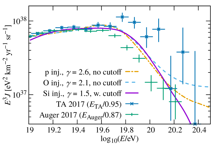
Figure 1: Energy spectra predicted at Earth in the three composition scenarios described in the text, from SimProp v2r4 simulations (Aloisio et al., 2017) assuming a uniform source distribution. TA data (Tsunesada, 2017) and Auger data (Fenu, 2017) are shown with energy scales shifted as recommended by Dembinski et al. (2017). The oxygen injection scenario includes secondary protons, whereas the silicon injection scenario does not due to the injection cutoff.

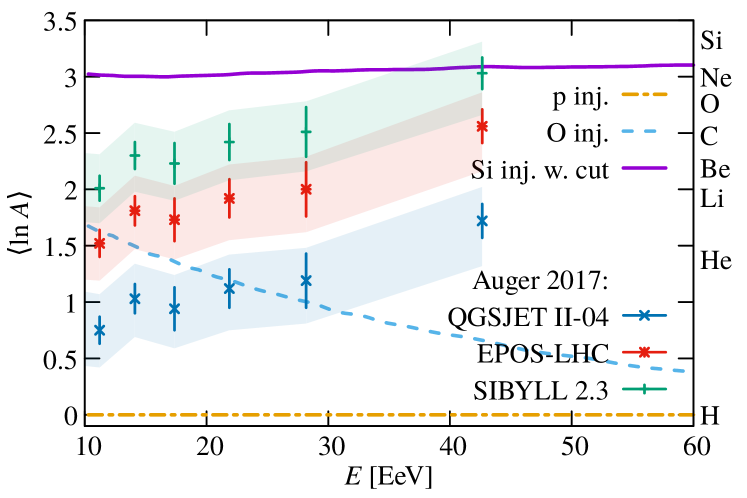
Figure 2: Average mass composition as a function of energy in our three scenarios, compared to Auger data as interpreted through three different hadronic interaction models (Bellido 2017; bars and shaded areas denote statistical and systematic uncertainties respectively).

In all three cases, we neglect any possible evolution of sources with cosmological time, because at these energies the vast majority of detected particles can be presumed to originate from sources at redshift $z\ll 1$.

Various energy loss processes reduce the number of protons or nuclei reaching our Galaxy with energy above a given threshold. On the other hand, in the case of injection of medium-mass nuclei with no injection cutoff, secondary protons from the spallation of the highest-energy nuclei are also produced. We used an approximation scheme described below to take into account these phenomena; we have verified that this yields results in agreement with those from full Monte Carlo simulations of UHECR propagation at the percent level.

One may assume that all nuclei of atomic weight $A$ injected with $E>10A$ EeV immediately disintegrate into $A$ protons each with energy $1/A$ times the initial energy of the nucleus, as at these energies the energy loss lengths for spallation by cosmic microwave background photons are a few Mpc or less, as is the beta-decay length of neutrons. In the case of a power-law injection of nuclei with no cutoff, this results in a number of secondary protons above a given threshold

$$N_{\mathrm{p}}(\geq E_{\min})=A^{2-\gamma}N_{A}(\geq E_{\min}).$$ (1)

The result is equivalent, in this approximation, to injecting directly a mixture of nuclei and protons in the proportion set by eq. (1). In the case $A=16$ and $\gamma=2.1$, the injected number fraction of protons is $\approx 57\%$ of the total.

Next, we have to take into account energy losses experienced by lower-energy nuclei and protons. These include the adiabatic energy loss due to the expansion of the Universe (redshift), interactions with background photons such as electron-positron pair production and pion production, and again spallation, this time mostly on infrared background photons. We do so via an attenuation function $a_{A}(E_{\min},D,\gamma)$ such that the number of nuclei (other than secondary nucleons) reaching our Galaxy with $E\geq E_{\min}$ from a source at a distance $D$ that emits nuclei of mass $A$ is $a_{A}(E_{\min},D,\gamma)$ times as much as if there were no energy losses. The attenuation of protons can likewise be described by a function $a_{\mathrm{p}}(E_{\min},D,\gamma)$.We need not take into account the secondary nucleons produced in the spallation of parent nuclei with $E<10A$ EeV, because those will all reach our Galaxy with energies below 10 EeV, which is the lowest energy we consider in this work. Therefore, in the silicon case no secondary nucleons are present. Also, most of the nuclei that undergo spallation but still reach our Galaxy with $E\geq 10$ EeV only lose a few nucleons at most, so we approximate them as all having the same electric charge as the primaries. The closeness of the $\langle\ln A\rangle$ line in Figure 2 for the silicon scenario to a constant $\ln 28\approx 3.3$ shows the goodness of this approximation.

In the oxygen case with no source cutoff, the flux arriving at our Galaxy in this approximation then consists of the leading $A$ nuclei attenuated by a factor $a_{A}(E_{\min},D,\gamma)$, and secondary protons, initially $A^{2-\gamma}$ times as many as the nuclei but then attenuated by a factor $a_{\mathrm{p}}(E_{\min},D,\gamma)$. In the proton and silicon case, only the protons or only the nuclei are present, respectively. We use parametrizations for $a_{A}(E_{\min},D,\gamma)$ and $a_{\mathrm{p}}(E_{\min},D,\gamma)$ fitted to results from SimProp v2r4 (Aloisio et al., 2017) simulations.

Finally, we have to estimate the contribution to the total flux at Earth of sources outside the catalog ($D>250$ Mpc), which we assume to be isotropic. We do so by defining a function $f_{A}(E_{\min},\gamma)$ as follows,

$$f_{A}(E_{\min},\gamma)=\frac{N_{A}(E_{\text{Earth}}\geq E_{\min},D\leq 250~{}\mathrm{Mpc})}{N_{A}(E_{\text{Earth}}\geq E_{\min},\text{all }D)}$$

in the hypothesis that sources emitting nuclei with mass number $A$ are uniformly distributed per unit comoving volume; we define an analogous function $f_{\mathrm{p}}(E_{\min},\gamma)$ for protons. We use parametrizations for $f_{A}(E_{\min},\gamma)$ and $f_{\mathrm{p}}(E_{\min},\gamma)$ fitted to results from SimProp v2r4 (Aloisio et al., 2017) simulations (Figure 3).

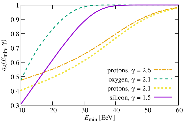
Figure 3: Fraction of nuclei (excluding secondary protons) having originated from within 250 Mpc among all those reaching Earth with $E\geq E_{\min}$, computed from SimProp v2r4 simulations (Aloisio et al., 2017) assuming a uniform source distribution

The total directional flux just outside the Galaxy is then the sum of four contributions (nuclei from catalog sources, nuclei from isotropic far sources, protons from catalog sources, protons from isotropic far sources), which we compute as

$$\Phi^{\text{cat}}_{A}({\mathbf{\hat{n}}},\geq E_{\min}) =N_{\mathrm{p}}(\geq E_{\min})\sum_{s}w_{s}\frac{a_{A}(D_{s})}{4\pi D_{s}^{2}}S({\mathbf{\hat{n}}},{\mathbf{\hat{n}}}_{s}),$$

$$\Phi^{\text{far}}_{A}({\mathbf{\hat{n}}},\geq E_{\min}) =\frac{1-f_{A}}{f_{A}}\frac{\int_{4\pi}{\Phi^{\text{cat}}_{A}({\mathbf{\hat{n}}})}\,\mathrm{d}\Omega}{4\pi},$$

$$\Phi^{\text{cat}}_{\mathrm{p}}({\mathbf{\hat{n}}},\geq E_{\min}) =N_{A}(\geq E_{\min})\sum_{s}w_{s}\frac{a_{\mathrm{p}}(D_{s})}{4\pi D_{s}^{2}}S({\mathbf{\hat{n}}},{\mathbf{\hat{n}}}_{s}),$$

$$\Phi^{\text{far}}_{\mathrm{p}}({\mathbf{\hat{n}}},\geq E_{\min}) =\frac{1-f_{\mathrm{p}}}{f_{\mathrm{p}}}\frac{\int_{4\pi}{\Phi^{\text{cat}}_{\mathrm{p}}({\mathbf{\hat{n}}})}\,\mathrm{d}\Omega}{4\pi},$$

where the index $s$ runs over sources, $w_{s}$ is a weight that takes into account the observational bias in the flux-limited catalog (see Koers & Tinyakov (2009) for details), the dependence of $f_{i}$ and $a_{i}$ on $\gamma$ and $E_{\min}$ is omitted for brevity, and $S({\mathbf{\hat{n}}},{\mathbf{\hat{n}}}_{s})\propto\exp({\mathbf{\hat{n}}}\cdot{\mathbf{\hat{n}}}_{s}/\sigma^{2})$ is a smearing function to take into account the finite detector angular resolution and deflections in random magnetic fields. In the proton case $N_{A}(\geq E_{\min})=0$, in the silicon case $N_{\mathrm{p}}(\geq E_{\min})=0$, and in the oxygen case they are related by eq. (1).

We compute such fluxes at several different values of $E_{\min}$, so that by subtracting them we can find the directional flux in each energy bin, and then compute magnetic deflections for each energy bin as described below.

2.3 Deflections in cosmic magnetic fields

The present constraints on the magnitude $B$ of the extragalactic field are at the level of $B\lesssim 1$nG (Pshirkov et al., 2016). With such a magnitude and a correlation length $l_{c}\sim 1$ Mpc, a nucleus with magnetic rigidity $E/Z=10$ EV (where $Z$ is the electric charge) would be deflected by approximately

$$\frac{2}{\pi}\frac{eB}{E/Z}\sqrt{l_{c}D}~{}\mathrm{rad}\approx 20^{\circ}\left(\frac{D}{50~{}\mathrm{Mpc}}\right)^{1/2},$$

$D$ being the distance to the source (Lee et al., 1995). Likely, for most of the directions the deflections are even smaller (Dolag et al., 2005).

The GMF is usually assumed to have regular and turbulent components. This field may be inferred from the Faraday rotations of galactic and extragalactic sources, synchrotron emission of relativistic electrons in the Galaxy, and polarized dust emission (see Haverkorn (2015) for a review). Two recent regular field models can be found in Pshirkov et al. (2011); Jansson & Farrar (2012); in what follows these will be referred to as PT2011 and JF2012, respectively. These models use different input data and a different global structure of the GMF. The predicted deflections are consistent in magnitude, having typical values $20\degr$–$40\degr$ for nuclei with rigidity $E/Z=10$ EV, but often differ in direction. The PT2011 model was only fitted to Faraday rotation data which are not sensitive to magnetic field components perpendicular to the line of sight, which are the most important for UHECR deflections, so the fact that even this model results in dipole and quadrupole magnitudes not very different from those from JF2012 is a strong indication of the robustness of our approach to uncertainties in the details of the GMF.

The turbulent component of GMF has a larger magnitude than the regular one, but a small ($\lesssim 100$ pc) coherence length makes the effect of this field subdominant when averaged over the particle trajectory. Quantitative estimates (Tinyakov & Tkachev, 2005; Pshirkov et al., 2013) indicate that the contribution of the turbulent field into the UHECR deflections is at least a factor $\sim 3$ smaller than that of the regular one except near the Galactic plane.

When simulating the expected UHECR flux we correct the flux maps for the deflections in the GMF. For the regular field we use both the PT2011 and JF2012 models; the difference between them gives an idea of the uncertainty resulting from the GMF modeling. The random field is accounted for by Gaussian smearing of the maps with the angular width given by the Pshirkov et al. (2013) upper bound,

$$\left(\frac{E/Z}{40~{}\mathrm{EV}}\right)^{-1}\frac{1^{\circ}}{\sin^{2}b+0.15},$$ (2)

which for nuclei with rigidity $E/Z=10$ EV ranges from $3.5^{\circ}$ at the Galactic poles to $27^{\circ}$ along the Galactic plane, implemented as described in appendix A.

3 Results

We have calculated the expected angular distribution of the arrival directions of UHECRs at Earth and the corresponding harmonic coefficients for the three scenarios described in subsection 2.2 and energy thresholds $E_{\min}$ between 10 and 60 EeV. We do not consider higher thresholds, because above the cutoff in the UHECR spectrum the statistics drops rapidly which makes the measurement of multipoles difficult. All calculations were repeated with the two GMF models.

We first present the flux sky maps of events above 60 EeV. The maps assuming a pure proton or silicon injection and the PT2011 GMF model are shown in Figure 4. The stronger large-scale anisotropy is obtained from the silicon injection with a cutoff, because the short energy loss lengths imply that the most of the flux originates from sources within a few tens of Mpc, where the matter distribution is dominated by a few large structures. Protons have longer energy loss lengths, so a larger number of structures, up to a couple hundred Mpc, can contribute. The magnetic deflections somewhat smear the picture at small angular scales, especially near the Galactic plane, being of a few degrees for protons and a few tens of degrees for silicon.

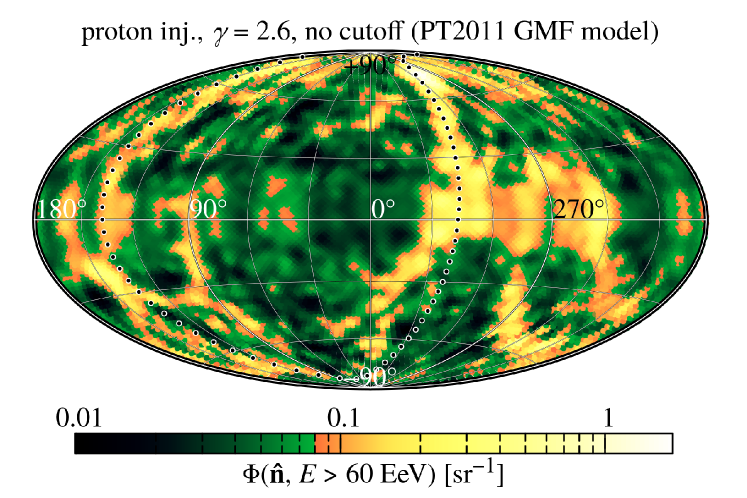
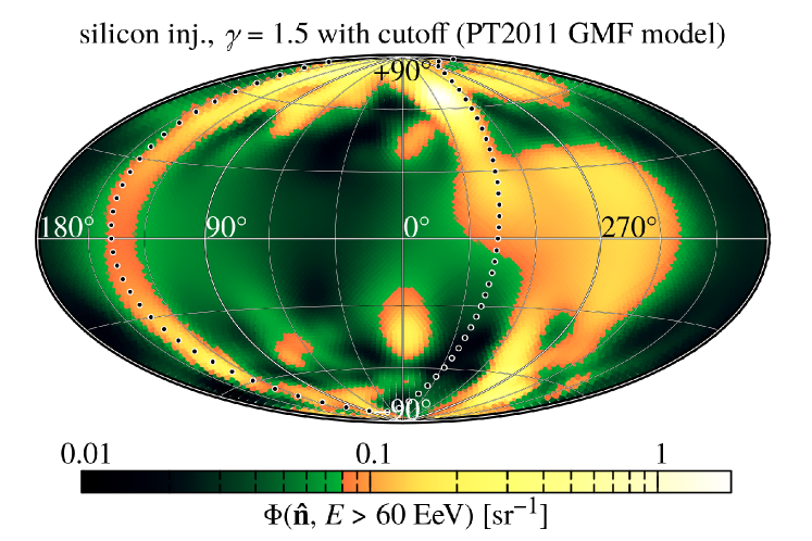
Figure 4: The expected angular distribution of UHECR arrival directions at Earth with energies above $60$ EeV for pure proton (top) or silicon (bottom) injection, assuming the PT2011 GMF model, in Galactic coordinates. The normalization is such that $\int_{4\pi}\Phi({\mathbf{\hat{n}}})\,\mathrm{d}\Omega=1$ (mean value $1/4\pi\approx 0.08$). Black dots show the supergalactic plane.

The case of oxygen injection with no cutoff is similar to that of protons, because the flux at high energies is dominated by the secondary protons.

At lower energies, the effect of magnetic deflections becomes much more important, up to several tens of degrees for protons and even larger for silicon. As shown in Figure 5, the structures visible in the previous plots get smeared and displaced. The overall contrast of these maps is smaller than in the previous case (note that the color codings for these plots are different, in order to make smaller flux variations more visible), especially for silicon, whose flux only varies by $\sim 10\%$ around the mean value $1/4\pi\approx 0.0796$ in most of the sky. There are two reasons for the lower contrast: larger smearing by magnetic deflections, and smaller relative contribution of nearby structures, as they get diluted by a (nearly) isotropic flux coming from distant sources due to slower attenuation at lower energies. The second effect is more important.

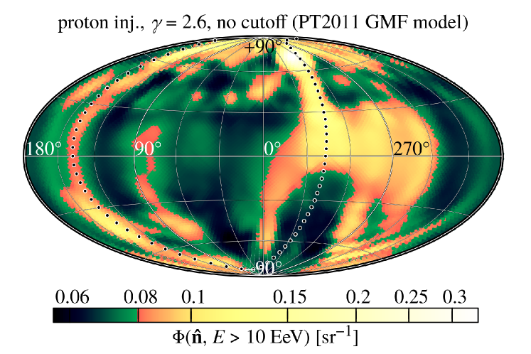
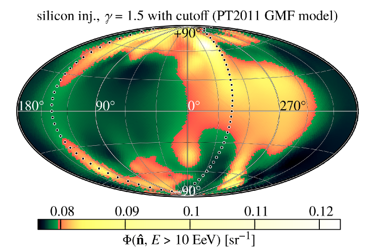
Figure 5: Sky maps of the expected UHECR directional flux above $10$ EeV for pure proton (top) or silicon (bottom) injection, assuming the PT2011 GMF model, normalized to $\int_{4\pi}\Phi({\mathbf{\hat{n}}})\,\mathrm{d}\Omega=1$ (mean value $1/4\pi\approx 0.0796$), in Galactic coordinates (same notation as in Figure 4, but different color scales)

The case of oxygen injection with no cutoff is intermediate between protons and silicon, as the total flux includes both the surviving nuclei (which have a smaller electric charge than silicon ones) and the secondary protons.

3.1 Dipole and quadrupole moments

To characterize the anisotropy quantitatively, we use the angular power spectrum

$$C_{l}=\frac{1}{2l+1}\sum_{m=-l}^{+l}|a_{lm}|^{2},$$

where $a_{lm}$ are the coefficients of the spherical harmonic expansion of the directional flux

$$\Phi({\mathbf{\hat{n}}})=\sum_{l=0}^{+\infty}\sum_{m=-l}^{+l}a_{lm}Y_{lm}({\mathbf{\hat{n}}}).$$

The angular power spectrum $C_{l}$ quantifies the amount of anisotropy at angular scales $\sim(\pi/l)$ rad and is rotationally invariant.

Explicitely, retaining only the dipole ($l=1$) and quadrupole ($l=2$) contributions, the flux $\Phi({\mathbf{\hat{n}}})$ can be written as

$$\Phi({\mathbf{\hat{n}}})=\Phi_{0}(1+\mathbf{d}\cdot{\mathbf{\hat{n}}}+{\mathbf{\hat{n}}}\cdot\textbf{{Q}}{\mathbf{\hat{n}}}+\cdots),$$

where the average flux is $\Phi_{0}=a_{00}/\sqrt{4\pi}$ ($\Phi_{0}=1/4\pi$ if we use the normalization $\int_{4\pi}\Phi({\mathbf{\hat{n}}})\,\mathrm{d}\Omega=1$), the dipole $\mathbf{d}$ is a vector with 3 independent components, which are linear combinations of $a_{1m}/a_{00}$, and the quadrupole Q is a rank-2 traceless symmetric tensor (i.e., its eigenvalues $\lambda_{+},\lambda_{0},\lambda_{-}$ sum to 0 and its eigenvectors $\mathbf{\hat{q}_{+}},\mathbf{\hat{q}_{0}},\mathbf{\hat{q}_{-}}$ are orthogonal) with 5 independent components, which are linear combinations of $a_{2m}/a_{00}$. The rotationally invariant combinations $|{\bf d}|=3\sqrt{C_{1}/C_{0}}$ and $\sqrt{\lambda_{+}^{2}+\lambda_{-}^{2}+\lambda_{0}^{2}}=5\sqrt{3C_{2}/2C_{0}}$ characterize the magnitude of the corresponding relative flux variations over the sphere. The dipole and quadrupole moments quantify anisotropies at scales $\sim 180\degr$ and $\sim 90\degr$ respectively, and are therefore relatively insensitive to magnetic deflections except at the lowest energies.

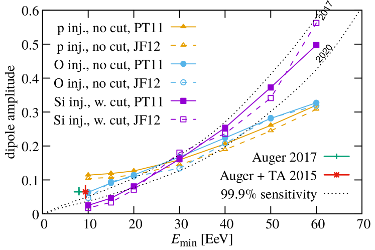
Figure 6: The magnitude of the dipole as a function of the energy threshold $E_{\min}$ for the three injection models and two GMF models we considered. The points labelled “Auger + TA 2015” and “Auger 2017” show the dipole magnitude reported in Deligny (2015) and Taborda (2017) respectively. The dotted lines show the 99.9% C.L. detection thresholds using the current and near-future Auger and TA exposures (see the text for details).

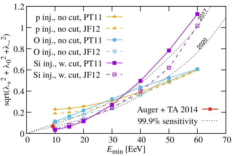
Figure 7: The magnitude of the dipole as a function of the energy threshold $E_{\min}$ (same notation as in Figure 6). The point labelled “Auger + TA 2014” is the quadrupole magnitude computed from the $a_{2m}$ coefficients reported in Aab et al. (2014).

In Figure 6 and Figure 7, we present the energy dependence of the dipole amplitude $|{\bf d}|$ and the quadrupole amplitude $(\lambda_{+}^{2}+\lambda_{-}^{2}+\lambda_{0}^{2})^{1/2}$ respectively in the various scenarios we considered. The first thing we point out is that, whereas there are some differences between predictions using the two different GMF models with the same injection model, they are not so large as to impede a meaningful interpretation of the results in spite of the GMF uncertainties. Conversely, the results from the three injection models do differ significantly, with heavier compositions resulting in larger dipole and quadrupole moments for high energy thresholds (due to the shorter propagation horizon) but smaller ones for lower thresholds (due to larger magnetic deflections).

Increasing the energy threshold, the expected dipole and quadrupole strengths increase, but at the same time the amount of statistics available decreases due to the steeply falling energy spectrum, making it non-obvious whether the overall effect is to make the detection of the dipole and quadrupole easier with higher or lower $E_{\min}$. To answer this question, we have calculated the 99.9% C.L. detection thresholds, i.e., the multipole amplitudes such that larger values would be measured in less than 0.1% of random realizations in case of a isotropic UHECR flux. The detection thresholds scale like $\propto 1/\sqrt{N}$ with the number of events $N$. Since below the observed cutoff ($\sim 40$ EeV) the integral spectrum at Earth $N(\geq E_{\min})$ is close to a power law $\propto E_{\min}^{-2}$, the detection threshold is roughly proportional to $E_{\min}$. At higher energies, the experimental sensitivity degrades faster as the result of the cutoff.

In order to compute the detection thresholds, we assumed the energy spectrum measured by Auger (Fenu, 2017) and: (i) the sum of the exposures used in the most recent Auger (Giaccari, 2017) and TA (Nonaka, 2017) analyses (lines labelled “2017”); (ii) the sum of the exposures expected if another $3$ yr of data are collected with $3\,000~{}\mathrm{km}^{2}$ effective area by each observatory, as planned following the fourfold expansion of TA (Sagawa, 2015) (lines labelled “2020”). The sensitivity is less than what it would be if we had uniform exposure over the full sky, as the actual exposure is currently much larger in the southern than in the northern hemisphere. Also, we neglected the systematic uncertainty due to the different energy scales of the two experiments, which mainly affects the $z$-component of the dipole. We find that the dipole and quadrupole strengths increase with the energy threshold faster than the statistical sensitivity degrades in the case of a heavy composition but slower in the case of a medium or light composition, making higher thresholds more advantageous in the former case, and lower thresholds in the latter.

At the highest energies (where there cannot be large amounts of intermediate-mass nuclei, due to photodisintegration), a heavy composition would result in a dipole and especially quadrupole moment large enough to be detected in the very near future; failure to do so would be strongly indicative of a proton-dominated composition at those energies.

At intermediate energies ($E_{\min}\sim 30$ EeV), the dipole and quadrupole are guaranteed to be above the near-future detection threshold regardless of the mass composition. Unfortunately the model predictions do not vary dramatically at these energies, so while a lack of dipole or quadrupole would imply that some of our assumptions must be wrong, a successful detection will not be particularly useful in discriminating between the various injection scenarios.

At even lower energy thresholds, the sensitivity of the dipole and quadrupole moment to the UHECR mass composition is again stronger; in particular, the combined Auger and TA dataset (Aab et al., 2014) is already able to disfavour a pure proton composition, as it would result in a much stronger quadrupole moment than observed, as shown by the corresponding data point in Figure 7. We also show the dipole magnitudes reported by TA and Auger for $E_{\min}=10$ EeV (Deligny, 2015) and by Auger only for $E_{\min}=8$ EeV (Taborda, 2017) in Figure 6. The latter has smaller error bars, but it is the result of an analysis relying on the hypothesis that the angular distribution is purely dipolar with zero quadrupole or higher moments, contrary to our model predictions of a quadrupole moment similar in magnitude to the dipole in all cases. The combined TA–Auger analysis, due to its full-sky coverage, does not require such a hypothesis.

4 Conclusions

To summarize, we have calculated a minimum level of anisotropy of the UHECR flux that is expected in a generic model where the sources trace the matter distribution in the nearby Universe, under the assumption that UHECRs above 10 EeV have a light or medium (but otherwise arbitrary) composition. To this end we calculated the expected angular distribution of UHECR arrival directions resulting from the corresponding distribution of sources in the case of a pure silicon injection (which maximizes the magnetic deflections) and a pure proton injection (which maximizes the contribution of distant, near-homogeneous sources), as well as an intermediate case (oxygen injection with secondary protons). To quantify the resulting anisotropy we have chosen the low multipole power spectrum coefficients $C_{l}$, namely the dipole and quadrupole moments, which are the least sensitive to the coherent magnetic deflections and the most easily measured. The uncertainties in the magnetic field modeling were roughly estimated by comparing two different GMF models. We also calculated the smallest dipole and quadrupole moments that could be unambiguously detected in present or near-future data.

Several conclusions follow from our results. First, there is a minimum amount of anisotropy that the UHECR flux must exhibit, regardless of the composition and the GMF details, provided our assumptions are correct: the dipole and quadrupole amplitudes above 30 EeV are expected to be $|{\bf d}|\gtrsim 0.13$ and $(\lambda_{+}^{2}+\lambda_{-}^{2}+\lambda_{0}^{2})^{1/2}\gtrsim 0.24$ in all cases. Second, larger statistics at low energies does not give a major advantage in the anisotropy detection (except for a proton-dominated composition) in the ideal situation, because the expected signal strength increases with energy roughly proportionally to the experimental sensitivity. (In the case of silicon injection, anisotropies at higher energies are even easier to detect than at lower energies.) Finally, in terms of detectability the quadrupole is about as good as the dipole, again in the ideal situation we have considered.

In reality, the terrestrial UHECR experiments do not have a complete sky coverage. To unambiguously measure the multipole coefficients one has to combine the TA and Auger data. Because of a possible systematic energy shift between the two experiments, a direct cross-calibration of fluxes is required (Aab et al., 2014). The cross-calibration introduces additional errors that affect more the dipole than the quadrupole measurement. Taking into account our results, this makes the quadrupole moment a more promising target to search for anisotropies resulting from an inhomogeneous distribution of matter in the Universe with the current configuration of the UHECR experiments. In particular, the non-observation of a strong quadrupole moment (Aab et al., 2014) already disfavors a pure proton composition.

The TA experiment is now being expanded to $\sim 4$ times the current size (Sagawa, 2015). After a few years of accumulation of events, the combined TA and Auger exposure will be much closer to a uniform one than at present. The detection threshold will then be close to the lower dotted line in Figs. 6 and 7. (Also, the planned upgrade of Auger will have dedicated detectors which will hopefully help us further reduce uncertainties on the UHECR mass composition (Aab et al., 2016).) The deviations from isotropy will either be detected then, or we will have to conclude that the UHECR deflections are much bigger than we infer from our current knowledge of the UHECR composition and cosmic magnetic fields.

Appendix A Implementation of deflections in the turbulent GMF

If the random diffusion of particles in the turbulent GMF were homogeneous and isotropic and its typical magnitude $\sigma$ were independent of the position in the sky, it could be simply be modelled by applying a Gaussian blur

$$\Phi_{\mathrm{new}}({\mathbf{\hat{n}}})=\int_{4\pi}\frac{1}{\pi\sigma^{2}}\exp\left(-\frac{|{\mathbf{\hat{n}}}-{\mathbf{\hat{n}}}^{\prime}|^{2}}{\sigma^{2}}\right)\Phi_{\mathrm{old}}({\mathbf{\hat{n}}}^{\prime})\,\mathrm{d}\Omega^{\prime}$$ (3)

to each flux map; but actually the deflections are larger near the Galactic plane than far away from it, as described by Equation 2.

As a result, it is not immediately obvious how to implement them; for example, if Equation 3 is used, either the smearing magnitude as a function of the undeflected direction $\sigma({\mathbf{\hat{n}}}^{\prime})$ or of the deflected direction $\sigma({\mathbf{\hat{n}}})$ might be used. At a closer look, the former procedure is clearly unphysical because it does not leave an isotropic flux map unchanged. On the other hand, the latter has the apparently counter-intuitive property that the image of a point source is not Gaussian. The exact motivation for the latter choice is also not clear, particularly at large deflection angles.

The correct procedure is obtained by noticing that, in the case of constant smearing angle, the full one-step smearing is equivalent to $N$ successive smearings with the smaller angle $\sigma/\sqrt{N}$. This is readily generalized to the angle-dependent case. Namely, we successively apply locally Gaussian smearings

$$\Phi_{i+1}({\mathbf{\hat{n}}})=\frac{1}{\pi{\sigma_{i}({\mathbf{\hat{n}}})}^{2}}\int_{4\pi}\Phi_{i}({\mathbf{\hat{n}}}^{\prime})\exp\left(-\frac{|{\mathbf{\hat{n}}}-{\mathbf{\hat{n}}}^{\prime}|^{2}}{\sigma_{i}({\mathbf{\hat{n}}})^{2}}\right)\,\mathrm{d}\Omega^{\prime}$$

with a smearing angle $\sigma_{i}({\mathbf{\hat{n}}})=\sigma({\mathbf{\hat{n}}})/\sqrt{N}$, where $\sigma({\mathbf{\hat{n}}})$ is given by Equation 2 and $N$ is the number of iterations. This mimics the actual physical process where the random deflections are not a one-step process and particles initially deflected towards the Galactic plane will likely end up deflected more than particles initially deflected away from it.

We found that the result is independent of $N$ provided it is large enough, and similar but not identical to smearing the map only once using the smearing angle as a function of the deflected direction $\sigma({\mathbf{\hat{n}}})$. The results we show in our plots were obtained with $N=9$. This also allowed us to compute each smearing via Monte Carlo integration (using for $\Phi_{i+1}({\mathbf{\hat{n}}})$ in each pixel the average of $\Phi_{i}({\mathbf{\hat{n}}}^{\prime})$ for 500 values of ${\mathbf{\hat{n}}}^{\prime}$ sampled from a Gaussian distribution around ${\mathbf{\hat{n}}}$) rather than a more time-consuming full numerical integration, after verifying in one case that the two methods give near-identical results for large $N$.

In Figure 8 we show the flux maps for $E_{\min}=10$ EeV in the silicon injection scenario (the one with the largest deflections) after zero, one, four and nine of the nine smearing steps used in Figure 5b.

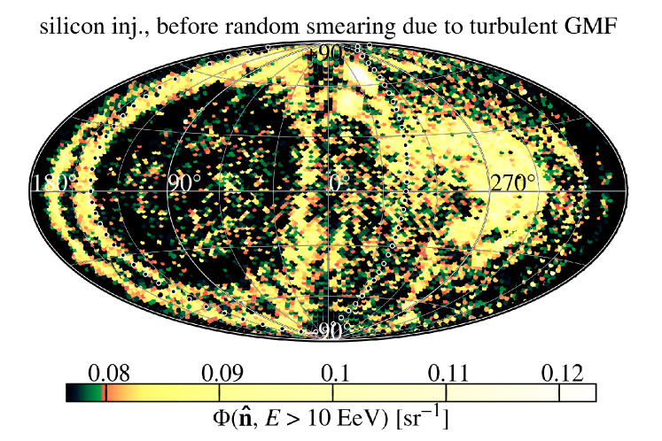
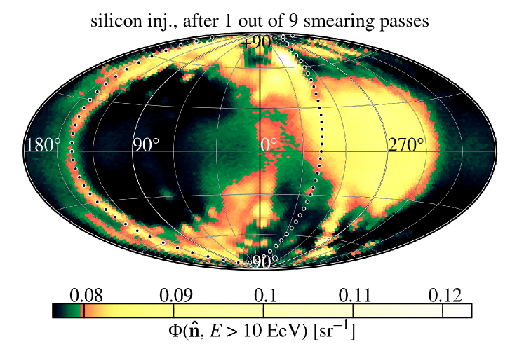
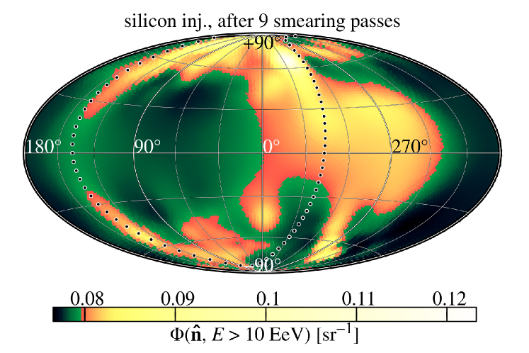
Figure 8: Flux maps as in Figure 5b, before the random smearing and after one, four and nine of the nine smearing steps used, using the same color scale

References

- Aab et al. (2014) Aab A. et al. (Pierre Auger and Telescope Array collabs.), 2014, ApJ, 794, 172
- Aab et al. (2015) Aab A. et al. (Pierre Auger collab.), 2015, Nucl. Instrum. Meth., A798, 172
- Aab et al. (2016) Aab A. et al. (Pierre Auger collab.), 2016, preprint (arXiv:1604.03637)
- Aab et al. (2017) Aab A. et al. (Pierre Auger collab.), 2017, J. Cosmol. Astropart. Phys., 04, 038
- Abbasi & Thomson (2016) Abbasi R. U., Thomson G. B., 2016, preprint (arXiv:1605.05241)
- Abbasi et al. (2014) Abbasi R. U. et al. (Telescope Array collab.), 2014, ApJ, 790, L21
- Abu-Zayyad et al. (2012) Abu-Zayyad T. et al. (Telescope Array collab.), 2012, ApJ, 757, 26
- Abu-Zayyad et al. (2013) Abu-Zayyad T. et al. (Telescope Array collab.), 2013, Nucl. Instrum. Meth., A689, 87
- Aloisio et al. (2017) Aloisio R., Boncioli D., di Matteo A., Grillo A. F., Petrera S., Salamida F., 2017, J. Cosmol. Astropart. Phys., 11, 009
- Bellido (2017) Bellido J. for the Pierre Auger collab., 2017, in Proc. 35th ICRC, 506
- Deligny (2015) Deligny O. for the Pierre Auger and Telescope Array collabs., 2015, in Proc. 34th ICRC, 395
- Dembinski et al. (2017) Dembinski H., Engel R., Fedynitch A., Gaisser T., Riehn F., Stanev T., 2017, in Proc. 35th ICRC, 533
- de Souza (2017) de Souza V. for the Pierre Auger and Telescope Array collabs., 2017, in Proc. 35th ICRC, 522
- di Matteo et al. (2018) di Matteo A. et al. for the Pierre Auger and Telescope Array collabs., 2018, JPS Conf. Proc., 19, 011020
- Dolag et al. (2005) Dolag K., Grasso D., Springel V., Tkachev I., 2005, J. Cosmol. Astropart. Phys., 01, 009
- Fenu (2017) Fenu F. for the Pierre Auger collab., 2017, in Proc. 35th ICRC, 486
- Giaccari (2017) Giaccari U. for the Pierre Auger collab., 2017, in Proc. 35th ICRC, 483
- Harari et al. (2014) Harari D., Mollerach S., Roulet E., 2014, Phys. Rev., D89, 123001
- Harari et al. (2015) Harari D., Mollerach S., Roulet E., 2015, Phys. Rev., D92, 063014
- Haverkorn (2015) Haverkorn M., 2015, in Lazarian A., de Gouveia Dal Pino E. M., Melioli C., eds, Astrophysics and Space Science Library Vol. 407, Magnetic Fields in Diffuse Media. p. 483 (arXiv:1406.0283), doi:10.1007/978-3-662-44625-6_17
- Jansson & Farrar (2012) Jansson R., Farrar G. R., 2012, ApJ, 757, 14
- Koers & Tinyakov (2009) Koers H. B. J., Tinyakov P., 2009, MNRAS, 399, 1005
- Koers & Tinyakov (2010) Koers H. B. J., Tinyakov P., 2010, MNRAS, 403, 2131
- Lee et al. (1995) Lee S., Olinto A. V., Sigl G., 1995, ApJ, 455, L21
- Mollerach et al. (2016) Mollerach S., Harari D., Roulet E., 2016, Nucl. Part. Phys. Proc., 273-275, 282
- Nonaka (2017) Nonaka T. for the Telescope Array collab., 2017, in Proc. 35th ICRC, 507
- Pshirkov et al. (2011) Pshirkov M. S., Tinyakov P. G., Kronberg P. P., Newton-McGee K. J., 2011, ApJ, 738, 192
- Pshirkov et al. (2013) Pshirkov M. S., Tinyakov P. G., Urban F. R., 2013, MNRAS, 436, 2326
- Pshirkov et al. (2016) Pshirkov M. S., Tinyakov P. G., Urban F. R., 2016, Phys. Rev. Lett., 116, 191302
- Rouillé d’Orfeuil et al. (2014) Rouillé d’Orfeuil B., Allard D., Lachaud C., Parizot E., Blaksley C., Nagataki S., 2014, A&A, 567, A81
- Sagawa (2015) Sagawa H. for the Telescope Array collab., 2015, in Proc. 34th ICRC, 657
- Sigl et al. (2003) Sigl G., Miniati F., Ensslin T. A., 2003, Phys. Rev., D68, 043002
- Sigl et al. (2004) Sigl G., Miniati F., Enßlin T. A., 2004, Phys. Rev., D70, 043007
- Skrutskie et al. (2006) Skrutskie M. F., et al., 2006, AJ, 131, 1163
- Taborda (2017) Taborda O. for the Pierre Auger collab., 2017, in Proc. 35th ICRC, 523
- Tinyakov & Tkachev (2005) Tinyakov P. G., Tkachev I. I., 2005, Astropart. Phys., 24, 32
- Tinyakov & Urban (2015) Tinyakov P. G., Urban F. R., 2015, J. Exp. Theor. Phys., 120, 533
- Tsunesada (2017) Tsunesada Y. for the Telescope Array collab., 2017, in Proc. 35th ICRC, 535
- Unger & Farrar (2017) Unger M., Farrar G. R., 2017, in Proc. 35th ICRC, 558