Self-Normalizing Neural Networks
Abstract
Deep Learning has revolutionized vision via convolutional neural networks (CNNs) and natural language processing via recurrent neural networks (RNNs). However, success stories of Deep Learning with standard feed-forward neural networks (FNNs) are rare. FNNs that perform well are typically shallow and, therefore cannot exploit many levels of abstract representations. We introduce self-normalizing neural networks (SNNs) to enable high-level abstract representations. While batch normalization requires explicit normalization, neuron activations of SNNs automatically converge towards zero mean and unit variance. The activation function of SNNs are “scaled exponential linear units” (SELUs), which induce self-normalizing properties. Using the Banach fixed-point theorem, we prove that activations close to zero mean and unit variance that are propagated through many network layers will converge towards zero mean and unit variance — even under the presence of noise and perturbations. This convergence property of SNNs allows to (1) train deep networks with many layers, (2) employ strong regularization schemes, and (3) to make learning highly robust. Furthermore, for activations not close to unit variance, we prove an upper and lower bound on the variance, thus, vanishing and exploding gradients are impossible. We compared SNNs on (a) 121 tasks from the UCI machine learning repository, on (b) drug discovery benchmarks, and on (c) astronomy tasks with standard FNNs, and other machine learning methods such as random forests and support vector machines. For FNNs we considered (i) ReLU networks without normalization, (ii) batch normalization, (iii) layer normalization, (iv) weight normalization, (v) highway networks, and (vi) residual networks. SNNs significantly outperformed all competing FNN methods at 121 UCI tasks, outperformed all competing methods at the Tox21 dataset, and set a new record at an astronomy data set. The winning SNN architectures are often very deep. Implementations are available at: github.com/bioinf-jku/SNNs.
Accepted for publication at NIPS 2017; please cite as:
Klambauer, G., Unterthiner, T., Mayr, A., & Hochreiter, S. (2017). Self-Normalizing Neural Networks. In Advances in Neural Information Processing Systems (NIPS).
Introduction
Deep Learning has set new records at different benchmarks and led to various commercial applications [25, 33]. Recurrent neural networks (RNNs) [18] achieved new levels at speech and natural language processing, for example at the TIMIT benchmark [12] or at language translation [36], and are already employed in mobile devices [31]. RNNs have won handwriting recognition challenges (Chinese and Arabic handwriting) [33, 13, 6] and Kaggle challenges, such as the “Grasp-and Lift EEG” competition. Their counterparts, convolutional neural networks (CNNs) [24] excel at vision and video tasks. CNNs are on par with human dermatologists at the visual detection of skin cancer [9]. The visual processing for self-driving cars is based on CNNs [19], as is the visual input to AlphaGo which has beaten one of the best human GO players [34]. At vision challenges, CNNs are constantly winning, for example at the large ImageNet competition [23, 16], but also almost all Kaggle vision challenges, such as the “Diabetic Retinopathy” and the “Right Whale” challenges [8, 14].
However, looking at Kaggle challenges that are not related to vision or sequential tasks, gradient boosting, random forests, or support vector machines (SVMs) are winning most of the competitions. Deep Learning is notably absent, and for the few cases where FNNs won, they are shallow. For example, the HIGGS challenge, the Merck Molecular Activity challenge, and the Tox21 Data challenge were all won by FNNs with at most four hidden layers. Surprisingly, it is hard to find success stories with FNNs that have many hidden layers, though they would allow for different levels of abstract representations of the input [3].
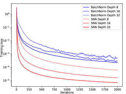
To robustly train very deep CNNs, batch normalization evolved into a standard to normalize neuron activations to zero mean and unit variance [20]. Layer normalization [2] also ensures zero mean and unit variance, while weight normalization [32] ensures zero mean and unit variance if in the previous layer the activations have zero mean and unit variance. However, training with normalization techniques is perturbed by stochastic gradient descent (SGD), stochastic regularization (like dropout), and the estimation of the normalization parameters. Both RNNs and CNNs can stabilize learning via weight sharing, therefore they are less prone to these perturbations. In contrast, FNNs trained with normalization techniques suffer from these perturbations and have high variance in the training error (see Figure 1). This high variance hinders learning and slows it down. Furthermore, strong regularization, such as dropout, is not possible as it would further increase the variance which in turn would lead to divergence of the learning process. We believe that this sensitivity to perturbations is the reason that FNNs are less successful than RNNs and CNNs.
Self-normalizing neural networks (SNNs) are robust to perturbations and do not have high variance in their training errors (see Figure 1). SNNs push neuron activations to zero mean and unit variance thereby leading to the same effect as batch normalization, which enables to robustly learn many layers. SNNs are based on scaled exponential linear units “SELUs” which induce self-normalizing properties like variance stabilization which in turn avoids exploding and vanishing gradients.
Self-normalizing Neural Networks (SNNs)
Normalization and SNNs.
For a neural network with activation function , we consider two consecutive layers that are connected by a weight matrix . Since the input to a neural network is a random variable, the activations in the lower layer, the network inputs , and the activations in the higher layer are random variables as well. We assume that all activations of the lower layer have mean and variance . An activation in the higher layer has mean and variance . Here denotes the expectation and the variance of a random variable. A single activation has net input . For units with activation in the lower layer, we define times the mean of the weight vector as and times the second moment as .
We consider the mapping that maps mean and variance of the activations from one layer to mean and variance of the activations in the next layer
| (1) |
Normalization techniques like batch, layer, or weight normalization ensure a mapping that keeps and close to predefined values, typically .
Definition 1 (Self-normalizing neural net).
A neural network is self-normalizing if it possesses a mapping for each activation that maps mean and variance from one layer to the next and has a stable and attracting fixed point depending on in . Furthermore, the mean and the variance remain in the domain , that is , where . When iteratively applying the mapping , each point within converges to this fixed point.
Therefore, we consider activations of a neural network to be normalized, if both their mean and their variance across samples are within predefined intervals. If mean and variance of are already within these intervals, then also mean and variance of remain in these intervals, i.e., the normalization is transitive across layers. Within these intervals, the mean and variance both converge to a fixed point if the mapping is applied iteratively.

Therefore, SNNs keep normalization of activations when propagating them through layers of the network. The normalization effect is observed across layers of a network: in each layer the activations are getting closer to the fixed point. The normalization effect can also observed be for two fixed layers across learning steps: perturbations of lower layer activations or weights are damped in the higher layer by drawing the activations towards the fixed point. If for all in the higher layer, and of the corresponding weight vector are the same, then the fixed points are also the same. In this case we have a unique fixed point for all activations . Otherwise, in the more general case, and differ for different but the mean activations are drawn into and the variances are drawn into .
Constructing Self-Normalizing Neural Networks.
We aim at constructing self-normalizing neural networks by adjusting the properties of the function . Only two design choices are available for the function : (1) the activation function and (2) the initialization of the weights.
For the activation function, we propose “scaled exponential linear units” (SELUs) to render a FNN as self-normalizing. The SELU activation function is given by
| (2) |
SELUs allow to construct a mapping with properties that lead to SNNs. SNNs cannot be derived with (scaled) rectified linear units (ReLUs), sigmoid units, units, and leaky ReLUs. The activation function is required to have (1) negative and positive values for controlling the mean, (2) saturation regions (derivatives approaching zero) to dampen the variance if it is too large in the lower layer, (3) a slope larger than one to increase the variance if it is too small in the lower layer, (4) a continuous curve. The latter ensures a fixed point, where variance damping is equalized by variance increasing. We met these properties of the activation function by multiplying the exponential linear unit (ELU) [7] with to ensure a slope larger than one for positive net inputs.
For the weight initialization, we propose and for all units in the higher layer. The next paragraphs will show the advantages of this initialization. Of course, during learning these assumptions on the weight vector will be violated. However, we can prove the self-normalizing property even for weight vectors that are not normalized, therefore, the self-normalizing property can be kept during learning and weight changes.
Deriving the Mean and Variance Mapping Function .
We assume that the are independent from each other but share the same mean and variance . Of course, the independence assumptions is not fulfilled in general. We will elaborate on the independence assumption below. The network input in the higher layer is for which we can infer the following moments and , where we used the independence of the . The net input is a weighted sum of independent, but not necessarily identically distributed variables , for which the central limit theorem (CLT) states that approaches a normal distribution: with density . According to the CLT, the larger , the closer is to a normal distribution. For Deep Learning, broad layers with hundreds of neurons are common. Therefore the assumption that is normally distributed is met well for most currently used neural networks (see Figure A8). The function maps the mean and variance of activations in the lower layer to the mean and variance of the activations in the next layer:
| (3) | ||||
These integrals can be analytically computed and lead to following mappings of the moments:
| (4) | ||||
| (5) | ||||
Stable and Attracting Fixed Point for Normalized Weights.
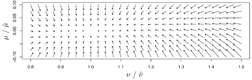
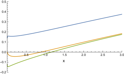
We assume a normalized weight vector with and . Given a fixed point , we can solve equations Eq. (4) and Eq. (5) for and . We chose the fixed point , which is typical for activation normalization. We obtain the fixed point equations and that we solve for and and obtain the solutions and , where the subscript indicates that these are the parameters for fixed point . The analytical expressions for and are given in Eq. (14). We are interested whether the fixed point is stable and attracting. If the Jacobian of has a norm smaller than 1 at the fixed point, then is a contraction mapping and the fixed point is stable. The (2x2)-Jacobian of evaluated at the fixed point with and is
| (6) |
The spectral norm of (its largest singular value) is . That means is a contraction mapping around the fixed point (the mapping is depicted in Figure 2). Therefore, is a stable fixed point of the mapping .
Stable and Attracting Fixed Points for Unnormalized Weights.
A normalized weight vector cannot be ensured during learning. For SELU parameters and , we show in the next theorem that if is close to , then still has an attracting and stable fixed point that is close to . Thus, in the general case there still exists a stable fixed point which, however, depends on . If we restrict to certain intervals, then we can show that is mapped to the respective intervals. Next we present the central theorem of this paper, from which follows that SELU networks are self-normalizing under mild conditions on the weights.
Theorem 1 (Stable and Attracting Fixed Points).
We assume and . We restrict the range of the variables to the following intervals , , , and , that define the functions’ domain . For and , the mapping Eq. (3) has the stable fixed point , whereas for other and the mapping Eq. (3) has a stable and attracting fixed point depending on in the -domain: and . All points within the -domain converge when iteratively applying the mapping Eq. (3) to this fixed point.
Proof.
We provide a proof sketch (see detailed proof in Appendix Section A3). With the Banach fixed point theorem we show that there exists a unique attracting and stable fixed point. To this end, we have to prove that a) is a contraction mapping and b) that the mapping stays in the domain, that is, . The spectral norm of the Jacobian of can be obtained via an explicit formula for the largest singular value for a matrix. is a contraction mapping if its spectral norm is smaller than . We perform a computer-assisted proof to evaluate the largest singular value on a fine grid and ensure the precision of the computer evaluation by an error propagation analysis of the implemented algorithms on the according hardware. Singular values between grid points are upper bounded by the mean value theorem. To this end, we bound the derivatives of the formula for the largest singular value with respect to . Then we apply the mean value theorem to pairs of points, where one is on the grid and the other is off the grid. This shows that for all values of in the domain , the spectral norm of is smaller than one. Therefore, is a contraction mapping on the domain . Finally, we show that the mapping stays in the domain by deriving bounds on and . Hence, the Banach fixed-point theorem holds and there exists a unique fixed point in that is attained. ∎
Consequently, feed-forward neural networks with many units in each layer and with the SELU activation function are self-normalizing (see definition 1), which readily follows from Theorem 1. To give an intuition, the main property of SELUs is that they damp the variance for negative net inputs and increase the variance for positive net inputs. The variance damping is stronger if net inputs are further away from zero while the variance increase is stronger if net inputs are close to zero. Thus, for large variance of the activations in the lower layer the damping effect is dominant and the variance decreases in the higher layer. Vice versa, for small variance the variance increase is dominant and the variance increases in the higher layer.
However, we cannot guarantee that mean and variance remain in the domain . Therefore, we next treat the case where are outside . It is especially crucial to consider because this variable has much stronger influence than . Mapping across layers to a high value corresponds to an exploding gradient, since the Jacobian of the activation of high layers with respect to activations in lower layers has large singular values. Analogously, mapping across layers to a low value corresponds to an vanishing gradient. Bounding the mapping of from above and below would avoid both exploding and vanishing gradients. Theorem 2 states that the variance of neuron activations of SNNs is bounded from above, and therefore ensures that SNNs learn robustly and do not suffer from exploding gradients.
Theorem 2 (Decreasing ).
For , and the domain : , , , and , we have for the mapping of the variance given in Eq. (5): .
The proof can be found in the Appendix Section A3. Thus, when mapped across many layers, the variance in the interval is mapped to a value below . Consequently, all fixed points of the mapping (Eq. (3)) have . Analogously, Theorem 3 states that the variance of neuron activations of SNNs is bounded from below, and therefore ensures that SNNs do not suffer from vanishing gradients.
Theorem 3 (Increasing ).
We consider , and the domain : , and . For the domain and as well as for the domain and , the mapping of the variance given in Eq. (5) increases: .
The proof can be found in the Appendix Section A3. All fixed points of the mapping (Eq. (3)) ensure for that and for that . Consequently, the variance mapping Eq. (5) ensures a lower bound on the variance . Therefore SELU networks control the variance of the activations and push it into an interval, whereafter the mean and variance move toward the fixed point. Thus, SELU networks are steadily normalizing the variance and subsequently normalizing the mean, too. In all experiments, we observed that self-normalizing neural networks push the mean and variance of activations into the domain .
Initialization.
Since SNNs have a fixed point at zero mean and unit variance for normalized weights and (see above), we initialize SNNs such that these constraints are fulfilled in expectation. We draw the weights from a Gaussian distribution with and variance . Uniform and truncated Gaussian distributions with these moments led to networks with similar behavior. The “MSRA initialization” is similar since it uses zero mean and variance to initialize the weights [17]. The additional factor counters the effect of rectified linear units.
New Dropout Technique.
Standard dropout randomly sets an activation to zero with probability for . In order to preserve the mean, the activations are scaled by during training. If has mean and variance , and the dropout variable follows a binomial distribution , then the mean is kept. Dropout fits well to rectified linear units, since zero is in the low variance region and corresponds to the default value. For scaled exponential linear units, the default and low variance value is . Therefore, we propose “alpha dropout”, that randomly sets inputs to . The new mean and new variance is , and . We aim at keeping mean and variance to their original values after “alpha dropout”, in order to ensure the self-normalizing property even for “alpha dropout”. The affine transformation allows to determine parameters and such that mean and variance are kept to their values: In contrast to dropout, and will depend on and , however our SNNs converge to activations with zero mean and unit variance. With and , we obtain and . The parameters and only depend on the dropout rate and the most negative activation . Empirically, we found that dropout rates or lead to models with good performance. “Alpha-dropout” fits well to scaled exponential linear units by randomly setting activations to the negative saturation value.
Applicability of the central limit theorem and independence assumption.
In the derivative of the mapping (Eq. (3)), we used the central limit theorem (CLT) to approximate the network inputs with a normal distribution. We justified normality because network inputs represent a weighted sum of the inputs , where for Deep Learning is typically large. The Berry-Esseen theorem states that the convergence rate to normality is [22]. In the classical version of the CLT, the random variables have to be independent and identically distributed, which typically does not hold for neural networks. However, the Lyapunov CLT does not require the variable to be identically distributed anymore. Furthermore, even under weak dependence, sums of random variables converge in distribution to a Gaussian distribution [5].
Experiments
We compare SNNs to other deep networks at different benchmarks. Hyperparameters such as number of layers (blocks), neurons per layer, learning rate, and dropout rate, are adjusted by grid-search for each dataset on a separate validation set (see Section A4). We compare the following FNN methods:
-
•
“MSRAinit”: FNNs without normalization and with ReLU activations and “Microsoft weight initialization” [17].
-
•
“BatchNorm”: FNNs with batch normalization [20].
-
•
“LayerNorm”: FNNs with layer normalization [2].
-
•
“WeightNorm”: FNNs with weight normalization [32].
-
•
“Highway”: Highway networks [35].
-
•
“ResNet”: Residual networks [16] adapted to FNNs using residual blocks with 2 or 3 layers with rectangular or diavolo shape.
-
•
“SNNs”: Self normalizing networks with SELUs with and and the proposed dropout technique and initialization strategy.
121 UCI Machine Learning Repository datasets.
The benchmark comprises 121 classification datasets from the UCI Machine Learning repository [10] from diverse application areas, such as physics, geology, or biology. The size of the datasets ranges between and data points and the number of features from to . In abovementioned work [10], there were methodological mistakes [37] which we avoided here. Each compared FNN method was optimized with respect to its architecture and hyperparameters on a validation set that was then removed from the subsequent analysis. The selected hyperparameters served to evaluate the methods in terms of accuracy on the pre-defined test sets (details on the hyperparameter selection are given in Section A4). The accuracies are reported in the Table A11. We ranked the methods by their accuracy for each prediction task and compared their average ranks. SNNs significantly outperform all competing networks in pairwise comparisons (paired Wilcoxon test across datasets) as reported in Table 1 (left panel).
| FNN method comparison | ML method comparison | ||||
|---|---|---|---|---|---|
| Method | avg. rank diff. | -value | Method | avg. rank diff. | -value |
| SNN | -0.756 | SNN | -6.7 | ||
| MSRAinit | -0.240* | 2.7e-02 | SVM | -6.4 | 5.8e-01 |
| LayerNorm | -0.198* | 1.5e-02 | RandomForest | -5.9 | 2.1e-01 |
| Highway | 0.021* | 1.9e-03 | MSRAinit | -5.4* | 4.5e-03 |
| ResNet | 0.273* | 5.4e-04 | LayerNorm | -5.3 | 7.1e-02 |
| WeightNorm | 0.397* | 7.8e-07 | Highway | -4.6* | 1.7e-03 |
| BatchNorm | 0.504* | 3.5e-06 | |||
We further included 17 machine learning methods representing diverse method groups [10] in the comparison and the grouped the data sets into “small” and “large” data sets (for details see Section A4). On 75 small datasets with less than 1000 data points, random forests and SVMs outperform SNNs and other FNNs. On 46 larger datasets with at least 1000 data points, SNNs show the highest performance followed by SVMs and random forests (see right panel of Table 1, for complete results see Tables A12 and A12). Overall, SNNs have outperformed state of the art machine learning methods on UCI datasets with more than 1,000 data points.
Typically, hyperparameter selection chose SNN architectures that were much deeper than the selected architectures of other FNNs, with an average depth of 10.8 layers, compared to average depths of 6.0 for BatchNorm, 3.8 WeightNorm, 7.0 LayerNorm, 5.9 Highway, and 7.1 for MSRAinit networks. For ResNet, the average number of blocks was 6.35. SNNs with many more than 4 layers often provide the best predictive accuracies across all neural networks.
Drug discovery: The Tox21 challenge dataset.
The Tox21 challenge dataset comprises about 12,000 chemical compounds whose twelve toxic effects have to be predicted based on their chemical structure. We used the validation sets of the challenge winners for hyperparameter selection (see Section A4) and the challenge test set for performance comparison. We repeated the whole evaluation procedure 5 times to obtain error bars. The results in terms of average AUC are given in Table 2. In 2015, the challenge organized by the US NIH was won by an ensemble of shallow ReLU FNNs which achieved an AUC of 0.846 [28]. Besides FNNs, this ensemble also contained random forests and SVMs. Single SNNs came close with an AUC of 0.8450.003. The best performing SNNs have 8 layers, compared to the runner-ups ReLU networks with layer normalization with 2 and 3 layers. Also batchnorm and weightnorm networks, typically perform best with shallow networks of 2 to 4 layers (Table 2). The deeper the networks, the larger the difference in performance between SNNs and other methods (see columns 5–8 of Table 2). The best performing method is an SNN with 8 layers.
| #layers / #blocks | |||||||
|---|---|---|---|---|---|---|---|
| method | 2 | 3 | 4 | 6 | 8 | 16 | 32 |
| SNN | 83.7 0.3 | 84.4 0.5 | 84.2 0.4 | 83.9 0.5 | 84.5 0.2 | 83.5 0.5 | 82.5 0.7 |
| Batchnorm | 80.0 0.5 | 79.8 1.6 | 77.2 1.1 | 77.0 1.7 | 75.0 0.9 | 73.7 2.0 | 76.0 1.1 |
| WeightNorm | 83.7 0.8 | 82.9 0.8 | 82.2 0.9 | 82.5 0.6 | 81.9 1.2 | 78.1 1.3 | 56.6 2.6 |
| LayerNorm | 84.3 0.3 | 84.3 0.5 | 84.0 0.2 | 82.5 0.8 | 80.9 1.8 | 78.7 2.3 | 78.8 0.8 |
| Highway | 83.3 0.9 | 83.0 0.5 | 82.6 0.9 | 82.4 0.8 | 80.3 1.4 | 80.3 2.4 | 79.6 0.8 |
| MSRAinit | 82.7 0.4 | 81.6 0.9 | 81.1 1.7 | 80.6 0.6 | 80.9 1.1 | 80.2 1.1 | 80.4 1.9 |
| ResNet | 82.2 1.1 | 80.0 2.0 | 80.5 1.2 | 81.2 0.7 | 81.8 0.6 | 81.2 0.6 | na |
Astronomy: Prediction of pulsars in the HTRU2 dataset.
Since a decade, machine learning methods have been used to identify pulsars in radio wave signals [27]. Recently, the High Time Resolution Universe Survey (HTRU2) dataset has been released with 1,639 real pulsars and 16,259 spurious signals. Currently, the highest AUC value of a 10-fold cross-validation is 0.976 which has been achieved by Naive Bayes classifiers followed by decision tree C4.5 with 0.949 and SVMs with 0.929. We used eight features constructed by the PulsarFeatureLab as used previously [27]. We assessed the performance of FNNs using 10-fold nested cross-validation, where the hyperparameters were selected in the inner loop on a validation set (for details on the hyperparameter selection see Section A4). Table 3 reports the results in terms of AUC. SNNs outperform all other methods and have pushed the state-of-the-art to an AUC of .
| FNN methods | FNN methods | ref. methods | |||||
|---|---|---|---|---|---|---|---|
| method | AUC | -value | method | AUC | -value | method | AUC |
| SNN | 0.9803 0.010 | ||||||
| MSRAinit | 0.9791 0.010 | 3.5e-01 | LayerNorm | 0.9762* 0.011 | 1.4e-02 | NB | 0.976 |
| WeightNorm | 0.9786* 0.010 | 2.4e-02 | BatchNorm | 0.9760 0.013 | 6.5e-02 | C4.5 | 0.946 |
| Highway | 0.9766* 0.009 | 9.8e-03 | ResNet | 0.9753* 0.010 | 6.8e-03 | SVM | 0.929 |
Conclusion
We have introduced self-normalizing neural networks for which we have proved that neuron activations are pushed towards zero mean and unit variance when propagated through the network. Additionally, for activations not close to unit variance, we have proved an upper and lower bound on the variance mapping. Consequently, SNNs do not face vanishing and exploding gradient problems. Therefore, SNNs work well for architectures with many layers, allowed us to introduce a novel regularization scheme, and learn very robustly. On 121 UCI benchmark datasets, SNNs have outperformed other FNNs with and without normalization techniques, such as batch, layer, and weight normalization, or specialized architectures, such as Highway or Residual networks. SNNs also yielded the best results on drug discovery and astronomy tasks. The best performing SNN architectures are typically very deep in contrast to other FNNs.
Acknowledgments
This work was supported by IWT research grant IWT150865 (Exaptation), H2020 project grant 671555 (ExCAPE), grant IWT135122 (ChemBioBridge), Zalando SE with Research Agreement 01/2016, Audi.JKU Deep Learning Center, Audi Electronic Venture GmbH, and the NVIDIA Corporation.
References
The references are provided in Section A7.
Appendix
This appendix is organized as follows: the first section sets the background, definitions, and formulations. The main theorems are presented in the next section. The following section is devoted to the proofs of these theorems. The next section reports additional results and details on the performed computational experiments, such as hyperparameter selection. The last section shows that our theoretical bounds can be confirmed by numerical methods as a sanity check.
The proof of theorem 1 is based on the Banach’s fixed point theorem for which we require (1) a contraction mapping, which is proved in Subsection A3.4.1 and (2) that the mapping stays within its domain, which is proved in Subsection A3.4.2 For part (1), the proof relies on the main Lemma 12, which is a computer-assisted proof, and can be found in Subsection A3.4.1. The validity of the computer-assisted proof is shown in Subsection A3.4.5 by error analysis and the precision of the functions’ implementation. The last Subsection A3.4.6 compiles various lemmata with intermediate results that support the proofs of the main lemmata and theorems.
A1 Background
We consider a neural network with activation function and two consecutive layers that are connected by weight matrix . Since samples that serve as input to the neural network are chosen according to a distribution, the activations in the lower layer, the network inputs , and activations in the higher layer are all random variables. We assume that all units in the lower layer have mean activation and variance of the activation and a unit in the higher layer has mean activation and variance . Here denotes the expectation and the variance of a random variable. For activation of unit , we have net input and the scaled exponential linear unit (SELU) activation , with
| (7) |
For units in the lower layer and the weight vector , we define times the mean by and times the second moment by .
We define a mapping from mean and variance of one layer to the mean and variance in the next layer:
| (8) |
For neural networks with scaled exponential linear units, the mean is of the activations in the next layer computed according to
| (9) |
and the second moment of the activations in the next layer is computed according to
| (10) |
Therefore, the expressions and have the following form:
| (11) | ||||
| (12) | ||||
| (13) | ||||
We solve equations Eq. 4 and Eq. 5 for fixed points and . For a normalized weight vector with and and the fixed point , we can solve equations Eq. 4 and Eq. 5 for and . We denote the solutions to fixed point by and .
| (14) | ||||
The parameters and ensure
Since we focus on the fixed point , we assume throughout the analysis that and . We consider the functions , , and on the domain .
Figure 2 visualizes the mapping for and and and at few pre-selected points. It can be seen that is an attracting fixed point of the mapping .
A2 Theorems
A2.1 Theorem 1: Stable and Attracting Fixed Points Close to (0,1)
Theorem 1 shows that the mapping defined by Eq. (4) and Eq. (5) exhibits a stable and attracting fixed point close to zero mean and unit variance. Theorem 1 establishes the self-normalizing property of self-normalizing neural networks (SNNs). The stable and attracting fixed point leads to robust learning through many layers.
Theorem 1 (Stable and Attracting Fixed Points).
We assume and . We restrict the range of the variables to the domain , , , and . For and , the mapping Eq. (4) and Eq. (5) has the stable fixed point . For other and the mapping Eq. (4) and Eq. (5) has a stable and attracting fixed point depending on in the -domain: and . All points within the -domain converge when iteratively applying the mapping Eq. (4) and Eq. (5) to this fixed point.
A2.2 Theorem 2: Decreasing Variance from Above
The next Theorem 2 states that the variance of unit activations does not explode through consecutive layers of self-normalizing networks. Even more, a large variance of unit activations decreases when propagated through the network. In particular this ensures that exploding gradients will never be observed. In contrast to the domain in previous subsection, in which , we now consider a domain in which the variance of the inputs is higher and even the range of the mean is increased . We denote this new domain with the symbol to indicate that the variance lies above the variance of the original domain . In , we can show that the variance in the next layer is always smaller then the original variance . Concretely, this theorem states that:
A2.3 Theorem 3: Increasing Variance from Below
The next Theorem 3 states that the variance of unit activations does not vanish through consecutive layers of self-normalizing networks. Even more, a small variance of unit activations increases when propagated through the network. In particular this ensures that vanishing gradients will never be observed. In contrast to the first domain, in which , we now consider two domains and in which the variance of the inputs is lower and , and even the parameter is different to the original . We denote this new domain with the symbol to indicate that the variance lies below the variance of the original domain . In and , we can show that the variance in the next layer is always larger then the original variance , which means that the variance does not vanish through consecutive layers of self-normalizing networks. Concretely, this theorem states that:
Theorem 3 (Increasing ).
We consider , and the two domains and .
A3 Proofs of the Theorems
A3.1 Proof of Theorem 1
We have to show that the mapping defined by Eq. (4) and Eq. (5) has a stable and attracting fixed point close to . To proof this statement and Theorem 1, we apply the Banach fixed point theorem which requires (1) that is a contraction mapping and (2) that does not map outside the function’s domain, concretely:
Theorem 4 (Banach Fixed Point Theorem).
Let be a non-empty complete metric space with a contraction mapping . Then has a unique fixed-point with . Every sequence with starting element converges to the fixed point: .
Contraction mappings are functions that map two points such that their distance is decreasing:
Definition 2 (Contraction mapping).
A function on a metric space with distance is a contraction mapping, if there is a , such that for all points and in : .
To show that is a contraction mapping in with distance , we use the Mean Value Theorem for
| (17) |
in which is an upper bound on the spectral norm the Jacobian of . The spectral norm is given by the largest singular value of the Jacobian of . If the largest singular value of the Jacobian is smaller than 1, the mapping of the mean and variance to the mean and variance in the next layer is contracting. We show that the largest singular value is smaller than 1 by evaluating the function for the singular value on a grid. Then we use the Mean Value Theorem to bound the deviation of the function between grid points. To this end, we have to bound the gradient of with respect to . If all function values plus gradient times the deltas (differences between grid points and evaluated points) is still smaller than 1, then we have proofed that the function is below 1 (Lemma 12). To show that the mapping does not map outside the function’s domain, we derive bounds on the expressions for the mean and the variance (Lemma 13). Section A3.4.1 and Section A3.4.2 are concerned with the contraction mapping and the image of the function domain of , respectively.
With the results that the largest singular value of the Jacobian is smaller than one (Lemma 12) and that the mapping stays in the domain (Lemma 13), we can prove Theorem 1. We first recall Theorem 1:
Theorem (Stable and Attracting Fixed Points).
We assume and . We restrict the range of the variables to the domain , , , and . For and , the mapping Eq. (4) and Eq. (5) has the stable fixed point . For other and the mapping Eq. (4) and Eq. (5) has a stable and attracting fixed point depending on in the -domain: and . All points within the -domain converge when iteratively applying the mapping Eq. (4) and Eq. (5) to this fixed point.
Proof.
According to Lemma 12 the mapping (Eq. (4) and Eq. (5)) is a contraction mapping in the given domain, that is, it has a Lipschitz constant smaller than one. We showed that is a fixed point of the mapping for .
The domain is compact (bounded and closed), therefore it is a complete metric space. We further have to make sure the mapping does not map outside its domain . According to Lemma 13, the mapping maps into the domain and .
Now we can apply the Banach fixed point theorem given in Theorem 4 from which the statement of the theorem follows. ∎
A3.2 Proof of Theorem 2
First we recall Theorem 2:
Theorem (Decreasing ).
Proof.
We start to consider an even larger domain , , , and . We prove facts for this domain and later restrict to , i.e. . We consider the function of the difference between the second moment in the next layer and the variance in the lower layer:
| (19) |
If we can show that for all , then we would obtain our desired result . The derivative with respect to is according to Theorem 16:
| (20) |
Therefore is strictly monotonically decreasing in . Since is a function in (these variables only appear as this product), we have for
| (21) |
and
| (22) |
Therefore we have according to Theorem 16:
| (23) |
Therefore
| (24) |
Consequently, is strictly monotonically increasing in . Now we consider the derivative with respect to and . We start with , which is
| (25) | ||||
We consider the sub-function
| (26) |
We set and and obtain
| (27) |
The derivative to this sub-function with respect to is
| (28) | |||
The inequality follows from Lemma 24, which states that is monotonically increasing in . Therefore the sub-function is increasing in . The derivative to this sub-function with respect to is
| (29) | |||
The sub-function is increasing in , since the derivative is larger than zero:
| (30) | |||
We explain this chain of inequalities:
-
•
First inequality: We applied Lemma 22 two times.
-
•
Equalities factor out and reformulate.
-
•
Second inequality part 1: we applied
(31) -
•
Second inequality part 2: we show that for following holds: . We have and . Therefore the minimum is at border for minimal and maximal :
(32) Thus
(33) for .
-
•
Equalities only solve square root and factor out the resulting terms and .
-
•
We set and multiplied out. Thereafter we also factored out in the numerator. Finally a quadratic equations was solved.
The sub-function has its minimal value for minimal and minimal . We further minimize the function
| (34) |
We compute the minimum of the term in brackets of in Eq. (25):
| (35) | |||
Therefore the term in brackets of Eq. (25) is larger than zero. Thus, has the sign of . Since is a function in (these variables only appear as this product), we have for
| (36) |
and
| (37) |
| (38) |
Since has the sign of , has the sign of . Therefore
| (39) |
has the sign of .
We now divide the -domain into and . Analogously we divide the -domain into and . In this domains is strictly monotonically.
For all domains is strictly monotonically decreasing in and strictly monotonically increasing in . Note that we now consider the range . For the maximal value of we set (we set it to 3!) and .
We consider now all combination of these domains:
-
•
and :
is decreasing in and decreasing in . We set and .
(40) -
•
and :
is increasing in and decreasing in . We set and .
(41) -
•
and :
is decreasing in and increasing in . We set and .
(42) -
•
and :
is increasing in and increasing in . We set and .
(43) Therefore the maximal value of is .
∎
A3.3 Proof of Theorem 3
First we recall Theorem 3:
Theorem (Increasing ).
We consider , and the two domains and .
Proof.
The mean value theorem states that there exists a for which
| (45) | |||
Therefore
| (46) | |||
Therefore we are interested to bound the derivative of the -mapping Eq. (13) with respect to :
| (47) | ||||
The sub-term Eq. (322) enters the derivative Eq. (47) with a negative sign! According to Lemma 18, the minimal value of sub-term Eq. (322) is obtained by the largest largest , by the smallest , and the largest . Also the positive term is multiplied by , which is minimized by using the smallest . Therefore we can use the smallest in whole formula Eq. (47) to lower bound it.
First we consider the domain and . The factor consisting of the exponential in front of the brackets has its smallest value for . Since is monotonically decreasing we inserted the smallest argument via in order to obtain the maximal negative contribution. Thus, applying Lemma 18, we obtain the lower bound on the derivative:
| (48) | |||
For applying the mean value theorem, we require the smallest . We follow the proof of Lemma 8, which shows that at the minimum must be maximal and must be minimal. Thus, the smallest is for and .
Therefore the mean value theorem and the bound on (Lemma 43) provide
| (49) | |||
Next we consider the domain and . The factor consisting of the exponential in front of the brackets has its smallest value for . Since is monotonically decreasing we inserted the smallest argument via in order to obtain the maximal negative contribution.
Thus, applying Lemma 18, we obtain the lower bound on the derivative:
| (50) | |||
For applying the mean value theorem, we require the smallest . We follow the proof of Lemma 8, which shows that at the minimum must be maximal and must be minimal. Thus, the smallest is for and . Therefore the mean value theorem and the bound on (Lemma 43) gives
| (51) | |||
∎
A3.4 Lemmata and Other Tools Required for the Proofs
A3.4.1 Lemmata for proofing Theorem 1 (part 1): Jacobian norm smaller than one
In this section, we show that the largest singular value of the Jacobian of the mapping is smaller than one. Therefore, is a contraction mapping. This is even true in a larger domain than the original . We do not need to restrict , but we can extend to . The range of the other variables is unchanged such that we consider the following domain throughout this section: , , , and .
Jacobian of the mapping.
In the following, we denote two Jacobians: (1) the Jacobian of the mapping , and (2) the Jacobian of the mapping because the influence of on is small, and many properties of the system can already be seen on .
| (56) | ||||
| (61) |
The definition of the entries of the Jacobian is:
| (62) | ||||
| (63) | ||||
| (64) | ||||
| (65) | ||||
Proof sketch: Bounding the largest singular value of the Jacobian.
If the largest singular value of the Jacobian is smaller than 1, then the spectral norm of the Jacobian is smaller than 1. Then the mapping Eq. (4) and Eq. (5) of the mean and variance to the mean and variance in the next layer is contracting.
We show that the largest singular value is smaller than 1 by evaluating the function on a grid. Then we use the Mean Value Theorem to bound the deviation of the function between grid points. Toward this end we have to bound the gradient of with respect to . If all function values plus gradient times the deltas (differences between grid points and evaluated points) is still smaller than 1, then we have proofed that the function is below 1.
The singular values of the matrix
| (68) |
are
| (69) | ||||
| (70) |
We used an explicit formula for the singular values [4]. We now set to obtain a formula for the largest singular value of the Jacobian depending on . The formula for the largest singular value for the Jacobian is:
| (71) | ||||
where are defined in Eq. (62) and we left out the dependencies on in order to keep the notation uncluttered, e.g. we wrote instead of .
Bounds on the derivatives of the Jacobian entries.
In order to bound the gradient of the singular value, we have to bound the derivatives of the Jacobian entries , , , and with respect to , , , and . The values and are fixed to and . The 16 derivatives of the 4 Jacobian entries with respect to the 4 variables are:
| (72) | ||||
Lemma 5 (Bounds on the Derivatives).
The following bounds on the absolute values of the derivatives of the Jacobian entries , , , and with respect to , , , and hold:
| (73) | ||||
Proof.
See proof 39. ∎
Bounds on the entries of the Jacobian.
Lemma 6 (Bound on J11).
The absolute value of the function
is bounded by
in the domain , , ,
and for and .
Proof.
where we used that (a) is strictly monotonically increasing in and and (b) Lemma 47 that ∎
Lemma 7 (Bound on J12).
The absolute value of the function
is bounded by
in the domain , , ,
and for and .
Proof.
| (75) |
For the first term we have after Lemma 47 and for the second term , which can easily be seen by maximizing or minimizing the arguments of the exponential or the square root function. The first term scaled by is and the second term scaled by is . Therefore, the absolute difference between these terms is at most leading to the derived bound.
∎
Bounds on mean, variance and second moment.
For deriving bounds on , , and , we need the following lemma.
Lemma 8 (Derivatives of the Mapping).
We assume and . We restrict the range of the variables to the domain , , , and .
The derivative has the sign of .
The derivative is positive.
The derivative has the sign of .
The derivative is positive.
Proof.
See 40. ∎
Lemma 9 (Bounds on mean, variance and second moment).
The expressions , , and for and are bounded by , and in the domain , , , .
Proof.
We use Lemma 8 which states that with given sign the derivatives of the mapping Eq. (4) and Eq. (5) with respect to and are either positive or have the sign of . Therefore with given sign of the mappings are strict monotonic and the their maxima and minima are found at the borders. The minimum of is obtained at and its maximum at and and at minimal or maximal values, respectively. It follows that
| (76) |
Similarly, the maximum and minimum of is obtained at the values mentioned above:
| (77) |
Hence we obtain the following bounds on :
| (78) | ||||
∎
Upper Bounds on the Largest Singular Value of the Jacobian.
Lemma 10 (Upper Bounds on Absolute Derivatives of Largest Singular Value).
We set and and restrict the range of the variables to , , , and .
The absolute values of derivatives of the largest singular value given in Eq. (71) with respect to are bounded as follows:
| (79) | ||||
| (80) | ||||
| (81) | ||||
| (82) |
Proof.
We obtain
| (89) | |||
and analogously
| (90) |
and
| (91) |
and
| (92) |
Derivative of the singular value w.r.t. :
| (98) | |||
Derivative of the singular value w.r.t. :
| (99) | |||
| (100) | |||
where we used the results from the lemmata 5, 6, 7, and 9 and that is symmetric for .
Derivative of the singular value w.r.t. :
| (101) | |||
Derivative of the singular value w.r.t. :
| (102) | |||
| (103) | |||
where we used the results from the lemmata 5, 6, 7, and 9 and that is symmetric for .
∎
Lemma 11 (Mean Value Theorem Bound on Deviation from Largest Singular Value).
We set and and restrict the range of the variables to , , , and .
The distance of the singular value at and that at is bounded as follows:
| (104) | |||
Proof.
The mean value theorem states that a exists for which
| (105) | |||
from which immediately follows that
| (106) | |||
We now apply Lemma 10 which gives bounds on the derivatives, which immediately gives the statement of the lemma. ∎
Lemma 12 (Largest Singular Value Smaller Than One).
We set and and restrict the range of the variables to , , , and .
Proof.
We set , , , and .
According to Lemma 11 we have
| (108) | ||||
For a grid with grid length , , , and , we evaluated the function Eq. (71) for the largest singular value in the domain , , , and . We did this using a computer. According to Subsection A3.4.5 the precision if regarding error propagation and precision of the implemented functions is larger than . We performed the evaluation on different operating systems and different hardware architectures including CPUs and GPUs. In all cases the function Eq. (71) for the largest singular value of the Jacobian is bounded by .
A3.4.2 Lemmata for proofing Theorem 1 (part 2): Mapping within domain
We further have to investigate whether the the mapping Eq. (4) and Eq. (5) maps into a predefined domains.
Lemma 13 (Mapping into the domain).
Proof.
We use Lemma 8 which states that with given sign the derivatives of the mapping Eq. (4) and Eq. (5) with respect to and are either positive or have the sign of . Therefore with given sign of the mappings are strict monotonic and the their maxima and minima are found at the borders. The minimum of is obtained at and its maximum at and and at their minimal and maximal values, respectively. It follows that:
| (110) |
and that .
Similarly, the maximum and minimum of is obtained at the values mentioned above:
| (111) |
Since , we can conclude that and the variance remains in . ∎
Corollary 14.
Proof.
Directly follows from Lemma 13. ∎
A3.4.3 Lemmata for proofing Theorem 2: The variance is contracting
Main Sub-Function.
We consider the main sub-function of the derivate of second moment, (Eq. (62)):
| (113) |
that depends on and , therefore we set and . Algebraic reformulations provide the formula in the following form:
| (114) |
For and , we consider the domain , , , and, .
For and we obtain: and . In the following we assume to remain within this domain.
Lemma 15 (Main subfunction).
For and ,
the function
| (115) |
is smaller than zero, is strictly monotonically increasing in , and strictly monotonically decreasing in for the minimal .
Proof.
See proof 44. ∎
The graph of the subfunction in the specified domain is displayed in Figure A3.

Theorem 16 (Contraction -mapping).
The mapping of the variance given in Eq. (5) is contracting for , and the domain : , , , and , that is,
| (116) |
Proof.
In this domain we have the following three properties (see further below): , , and . Therefore, we have
| (117) |
-
•
We first proof that in an even larger domain that fully contains . According to Eq. (62), the derivative of the mapping Eq. (5) with respect to the variance is
(118) For , , , , and , we first show that the derivative is positive and then upper bound it.
According to Lemma 15, the expression
(119) is negative. This expression multiplied by positive factors is subtracted in the derivative Eq. (118), therefore, the whole term is positive. The remaining term
(120) of the derivative Eq. (118) is also positive according to Lemma 21. All factors outside the brackets in Eq. (118) are positive. Hence, the derivative Eq. (118) is positive.
The upper bound of the derivative is:
(121) We explain the chain of inequalities:
- –
-
–
First inequality: The overall factor is bounded by 1.25.
-
–
Second inequality: We apply Lemma 15. According to Lemma 15 the function Eq. (115) is negative. The largest contribution is to subtract the most negative value of the function Eq. (115), that is, the minimum of function Eq. (115). According to Lemma 15 the function Eq. (115) is strictly monotonically increasing in and strictly monotonically decreasing in for . Therefore the function Eq. (115) has its minimum at minimal and maximal . We insert these values into the expression.
-
–
Third inequality: We use for the whole expression the maximal factor by setting this factor to 1.
-
–
Fourth inequality: is strictly monotonically decreasing. Therefore we maximize its argument to obtain the least value which is subtracted. We use the minimal and the maximal .
-
–
Sixth inequality: evaluation of the terms.
-
•
We now show that . The expression (Eq. (4)) is strictly monotonically increasing im and . Therefore, the minimal value in is obtained at .
-
•
Last we show that . The expression (Eq. (62)) can we reformulated as follows:
(122) is larger than zero when the term is larger than zero. This term obtains its minimal value at and , which can easily be shown using the Abramowitz bounds (Lemma 22) and evaluates to , therefore in .
∎
A3.4.4 Lemmata for proofing Theorem 3: The variance is expanding
Main Sub-Function From Below.
We consider functions in and , therefore we set and .
For and , we consider the domain , , and .
For and we obtain: and . In the following we assume to be within this domain.
In this domain, we consider the main sub-function of the derivate of second moment in the next layer, (Eq. (62)):
| (123) |
that depends on and , therefore we set and . Algebraic reformulations provide the formula in the following form:
| (124) | |||
Lemma 17 (Main subfunction Below).
For and , the function
| (125) |
smaller than zero, is strictly monotonically increasing in and strictly monotonically increasing in for the minimal , , , and (lower bound of on ).
Proof.
See proof 45. ∎
Lemma 18 (Monotone Derivative).
For , and the domain , , , and . We are interested of the derivative of
| (126) |
The derivative of the equation above with respect to
-
•
is larger than zero;
-
•
is smaller than zero for maximal , , and (with );
-
•
is larger than zero for , , , and .
Proof.
See proof 46. ∎
A3.4.5 Computer-assisted proof details for main Lemma 12 in Section A3.4.1.
Error Analysis.
We investigate the error propagation for the singular value (Eq. (71)) if the function arguments suffer from numerical imprecisions up to . To this end, we first derive error propagation rules based on the mean value theorem and then we apply these rules to the formula for the singular value.
Lemma 19 (Mean value theorem).
For a real-valued function which is differentiable in the closed interval , there exists with
| (127) |
It follows that for computation with error , there exists a with
| (128) |
Therefore the increase of the norm of the error after applying function is bounded by the norm of the gradient .
We now compute for the functions, that we consider their gradient and its 2-norm:
-
•
addition:
and , which gives .
We further know that
(129) Adding terms gives:
(130) -
•
subtraction:
and , which gives .
We further know that
(131) Subtracting terms gives:
(132) -
•
multiplication:
and , which gives .
We further know that
(133) Multiplying terms gives:
(134) -
•
division:
and , which gives .
We further know that
(135) -
•
square root:
and , which gives .
-
•
exponential function:
and , which gives .
-
•
error function:
and , which gives .
-
•
complementary error function:
and , which gives .
Lemma 20.
This means for a machine with a typical precision of , we have the rounding error , the evaluation of the singular value (Eq. (71)) with the formulas given in Eq. (62) and Eq. (71) has a precision better than .
Proof.
We have the numerical precision of the parameters , that we denote by together with our domain .
With the error propagation rules that we derived in Subsection A3.4.5, we can obtain bounds for the numerical errors on the following simple expressions:
| (136) | ||||
Using these bounds on the simple expressions, we can now calculate bounds on the numerical errors of compound expressions:
| (137) | ||||
| (138) | ||||
| (139) | ||||
| (140) |
Subsequently, we can use the above results to get bounds for the numerical errors on the Jacobian entries (Eq. (62)), applying the rules from Subsection A3.4.5 again:
| (141) |
and we obtain , , and . We also have bounds on the absolute values on and (see Lemma 6, Lemma 7, and Lemma 9), therefore we can propagate the error also through the function that calculates the singular value (Eq. (71)).
| (142) | |||
∎
Precision of Implementations.
We will show that our computations are correct up to 3 ulps. For our implementation in GNU C library and the hardware architectures that we used, the precision of all mathematical functions that we used is at least one ulp. The term “ulp” (acronym for “unit in the last place”) was coined by W. Kahan in 1960. It is the highest precision (up to some factor smaller 1), which can be achieved for the given hardware and floating point representation.
Kahan defined ulp as [21]:
“Ulp is the gap between the two finite floating-point numbers nearest , even if is one of them. (But ulp(NaN) is NaN.)”
Harrison defined ulp as [15]:
“an ulp in is the distance between the two closest straddling floating point numbers and , i.e. those with and assuming an unbounded exponent range.”
In the literature we find also slightly different definitions [29].
According to [29] who refers to [11]:
“IEEE-754 mandates four standard rounding modes:”
“Round-to-nearest: is the floating-point value closest to with the usual distance; if two floating-point value are equally close to , then is the one whose least significant bit is equal to zero.”
“IEEE-754 standardises 5 operations: addition (which we shall note in order to distinguish it from the operation over the reals), subtraction (), multiplication (), division (), and also square root.”
“IEEE-754 specifies em exact rounding [Goldberg, 1991, §1.5]: the result of a floating-point operation is the same as if the operation were performed on the real numbers with the given inputs, then rounded according to the rules in the preceding section. Thus, is defined as , with and taken as elements of ; the same applies for the other operators.”
Consequently, the IEEE-754 standard guarantees that addition, subtraction, multiplication, division, and squared root is precise up to one ulp.
We have to consider transcendental functions. First the is the exponential function, and then the complementary error function , which can be computed via the error function .
Intel states [29]:
“With the Intel486 processor and Intel 387 math coprocessor, the worst- case, transcendental function error is typically or ulps, but is some- times as large as ulps.”
According to https://www.mirbsd.org/htman/i386/man3/exp.htm and http://man.openbsd.org/OpenBSD-current/man3/exp.3:
“exp, log, expm1 and log1p are accurate to within an ulp”
which is the same for freebsd https://www.freebsd.org/cgi/man.cgi?query=exp&sektion=3&apropos=0&manpath=freebsd:
“The values of exp(0), expm1(0), exp2(integer), and pow(integer, integer) are exact provided that they are representable. Otherwise the error in these functions is generally below one ulp.”
The same holds for “FDLIBM” http://www.netlib.org/fdlibm/readme:
“FDLIBM is intended to provide a reasonably portable (see assumptions below), reference quality (below one ulp for major functions like sin,cos,exp,log) math library (libm.a).”
In http://www.gnu.org/software/libc/manual/html_node/Errors-in-Math-Functions.html we find that both and have an error of 1 ulp while has an error up to 3 ulps depending on the architecture. For the most common architectures as used by us, however, the error of is 1 ulp.
We implemented the function in the programming language C. We rely on the GNU C Library [26]. According to the GNU C Library manual which can be obtained from http://www.gnu.org/software/libc/manual/pdf/libc.pdf, the errors of the math functions , , and are not larger than 3 ulps for all architectures [26, pp. 528]. For the architectures ix86, i386/i686/fpu, and m68k/fpmu68k/m680x0/fpu that we used the error are at least one ulp [26, pp. 528].
A3.4.6 Intermediate Lemmata and Proofs
Since we focus on the fixed point , we assume for our whole analysis that and . Furthermore, we restrict the range of the variables , , , and .
For bounding different partial derivatives we need properties of different functions. We will bound a the absolute value of a function by computing an upper bound on its maximum and a lower bound on its minimum. These bounds are computed by upper or lower bounding terms. The bounds get tighter if we can combine terms to a more complex function and bound this function. The following lemmata give some properties of functions that we will use in bounding complex functions.
Throughout this work, we use the error function and the complementary error function .
Lemma 21 (Basic functions).
is strictly monotonically increasing from at to at and has positive curvature.
According to its definition is strictly monotonically decreasing from 2 at to 0 at .
Next we introduce a bound on :
Lemma 22 (Erfc bound from Abramowitz).
| (143) |
for .
Proof.
The statement follows immediately from [1] (page 298, formula 7.1.13). ∎
These bounds are displayed in figure A4.
Lemma 23 (Function ).
is strictly monotonically decreasing for and has positive curvature (positive 2nd order derivative), that is, the decreasing slowes down.


A graph of the function is displayed in Figure A5.
Proof.
The derivative of is
| (144) |
Using Lemma 22, we get
| (145) |
Thus is strictly monotonically decreasing for .
The second order derivative of is
| (146) |
Again using Lemma 22 (first inequality), we get
| (147) | |||
For the last inequality we added 1 in the numerator in the square root which is subtracted, that is, making a larger negative term in the numerator. ∎
Lemma 24 (Properties of ).
The function has the sign of and is monotonically increasing to .
Proof.
The derivative of is
| (148) |
This derivative is positive since
| (149) | |||
We apply Lemma 22 to and divide the terms of the lemma by , which gives
| (150) |
For both the upper and the lower bound go to . ∎
Lemma 25 (Function ).
is monotonically increasing in . It has minimal value and maximal value .
Proof.
Obvious. ∎
Lemma 26 (Function ).
is monotonically increasing in and is positive. It has minimal value and maximal value .
Proof.
Obvious. ∎
Lemma 27 (Function ).
is larger than zero and increasing in both and . It has minimal value and maximal value .
Proof.
The derivative of the function with respect to is
| (151) |
since and . ∎
Lemma 28 (Function ).
is larger than zero and increasing in both and . It has minimal value and maximal value .
Proof.
The derivative of the function with respect to is
| (152) |
∎
Lemma 29 (Function ).
monotonically decreasing in and monotonically increasing in . It has minimal value and maximal value .
Proof.
Obvious. ∎
Lemma 30 (Function ).
has a minimum at 0 for or and has a maximum for the smallest and largest and is larger or equal to zero. It has minimal value and maximal value .
Proof.
Obvious. ∎
Lemma 31 (Function ).
and decreasing in .
Proof.
Statements follow directly from elementary functions square root and division. ∎
Lemma 32 (Function ).
and decreasing in and increasing in .
Proof.
Statements follow directly from Lemma 21 and . ∎
Lemma 33 (Function ).
For and , and increasing in both and .
Proof.
We consider the function , which has the derivative with respect to :
| (153) |
This derivative is larger than zero, since
| (154) |
The last inequality follows from for .
We next consider the function , which has the derivative with respect to :
| (155) |
∎
Lemma 34 (Function ).
The function
is decreasing in and increasing in .
Proof.
We define the function
| (156) |
which has as derivative with respect to :
| (157) | |||
The derivative of the term with respect to is , since . Therefore the term is maximized with the smallest value for , which is . For we use for each term the value which gives maximal contribution. We obtain an upper bound for the term:
| (158) |
Therefore the derivative with respect to is smaller than zero and the original function is decreasing in
We now consider the derivative with respect to . The derivative with respect to of the function
| (159) |
is
| (160) |
Since , the derivative is larger than zero. Consequently, the original function is increasing in .
The maximal value is obtained with the minimal and the maximal . The maximal value is
| (161) |
Therefore the original function is smaller than zero. ∎
Lemma 35 (Function ).
For and ,
and increasing in both and .
Proof.
The derivative of the function
| (162) |
with respect to is
| (163) |
since
The derivative of the function
| (164) |
with respect to is
| (165) |
The maximal function value is obtained by maximal and the maximal . The maximal value is . Therefore the function is negative. ∎
Lemma 36 (Function ).
The function is decreasing in and increasing in .
Proof.
The derivative of the function
| (166) |
with respect to is
| (167) |
since .
The derivative of the function
| (168) |
with respect to is
| (169) |
The maximal function value is obtained for minimal and the maximal . The value is . Thus, the function is negative. ∎
Lemma 37 (Function ).
The function is increasing in and decreasing in .
Proof.
The derivative of the function
| (170) |
with respect to is
| (171) |
This derivative is larger than zero, since
| (172) | |||
We explain this chain of inequalities:
-
•
The first inequality follows by applying Lemma 23 which says that is strictly monotonically decreasing. The minimal value that is larger than 0.4349 is taken on at the maximal values and .
-
•
The second inequality uses .
-
•
The equalities are just algebraic reformulations.
-
•
The last inequality follows from .
Therefore the function is increasing in .
Decreasing in follows from decreasing of according to Lemma 23. Positivity follows form the fact that and the exponential function are positive and that . ∎
Lemma 38 (Function ).
The function is increasing in and decreasing in .
Proof.
The derivative of the function
| (173) |
is
| (174) |
We only have to determine the sign of since all other factors are obviously larger than zero.
This derivative is larger than zero, since
| (175) | |||
We explain this chain of inequalities:
-
•
The first inequality follows by applying Lemma 23 which says that is strictly monotonically decreasing. The minimal value that is larger than 0.261772 is taken on at the maximal values and . .
-
•
The equalities are just algebraic reformulations.
-
•
The last inequality follows from .
Therefore the function is increasing in .
Decreasing in follows from decreasing of according to Lemma 23. Positivity follows from the fact that and the exponential function are positive and that . ∎
Lemma 39 (Bounds on the Derivatives).
The following bounds on the absolute values of the derivatives of the Jacobian entries , , , and with respect to , , , and hold:
| (176) | ||||
Proof.
For each derivative we compute a lower and an upper bound and take the maximum of the absolute value. A lower bound is determined by minimizing the single terms of the functions that represents the derivative. An upper bound is determined by maximizing the single terms of the functions that represent the derivative. Terms can be combined to larger terms for which the maximum and the minimum must be known. We apply many previous lemmata which state properties of functions representing single or combined terms. The more terms are combined, the tighter the bounds can be made.
Next we go through all the derivatives, where we use Lemma 25, Lemma 26, Lemma 27, Lemma 28, Lemma 29, Lemma 30, Lemma 21, and Lemma 23 without citing. Furthermore, we use the bounds on the simple expressions ,, …, and as defined the aforementioned lemmata:
-
•
We use Lemma 31 and consider the expression in brackets. An upper bound on the maximum of is
(177) A lower bound on the minimum is
(178) Thus, an upper bound on the maximal absolute value is
(179) -
•
We use Lemma 31 and consider the expression in brackets.
An upper bound on the maximum is
(180) A lower bound on the minimum is
(181) This term is subtracted, and , therefore we have to use the minimum and the maximum for the argument of .
Thus, an upper bound on the maximal absolute value is
(182) -
•
We consider the term in brackets
(183) We apply Lemma 33 for the first sub-term. An upper bound on the maximum is
(184) A lower bound on the minimum is
(185) Thus, an upper bound on the maximal absolute value is
(186) -
•
We use the results of item were the brackets are only differently scaled. Thus, an upper bound on the maximal absolute value is
(187) -
•
Since , an upper bound on the maximal absolute value is
(188) -
•
We use the results of item were the brackets are only differently scaled. Thus, an upper bound on the maximal absolute value is
(189) -
•
For the second term in brackets, we see that and .
We now check different values for
(190) where we maximize or minimize all single terms.
A lower bound on the minimum of this expression is
(191) An upper bound on the maximum of this expression is
(192) An upper bound on the maximum is
(193) A lower bound on the minimum is
(194) Thus, an upper bound on the maximal absolute value is
(195) -
•
We use Lemma 34 to obtain an upper bound on the maximum of the expression of the lemma:
(196) We use Lemma 34 to obtain an lower bound on the minimum of the expression of the lemma:
(197) Next we apply Lemma 37 for the expression . We use Lemma 37 to obtain an upper bound on the maximum of this expression:
(198) We use Lemma 37 to obtain an lower bound on the minimum of this expression:
(199) Next we apply Lemma 23 for . An upper bound on this expression is
(200) A lower bound on this expression is
(201) The sum of the minimal values of the terms is .
The sum of the maximal values of the terms is .
Thus, an upper bound on the maximal absolute value is
(202) -
•
An upper bound on the maximum is
(203) A upper bound on the absolute minimum is
(204) Thus, an upper bound on the maximal absolute value is
(205) -
•
An upper bound on the maximum is
(206) A lower bound on the minimum is
(207) Thus, an upper bound on the maximal absolute value is
(208) -
•
An upper bound on the maximum is
(209) A lower bound on the minimum is
(210) Thus, an upper bound on the maximal absolute value is
(211) -
•
An upper bound on the maximum is
(212) A lower bound on the minimum is
(213) Thus, an upper bound on the maximal absolute value is
(214) -
•
We use the fact that . Thus, an upper bound on the maximal absolute value is
(215) -
•
An upper bound on the maximum is
(216) A lower bound on the minimum is
(217) Thus, an upper bound on the maximal absolute value is
(218) -
•
-
•
We apply Lemma 36 to the expression .
We apply Lemma 37 to the expression . We apply Lemma 38 to the expression .We combine the results of these lemmata to obtain an upper bound on the maximum:
(222) We combine the results of these lemmata to obtain an lower bound on the minimum:
(223) Thus, an upper bound on the maximal absolute value is
(224)
∎
Lemma 40 (Derivatives of the Mapping).
We assume and . We restrict the range of the variables to the domain , , , and .
The derivative has the sign of .
The derivative is positive.
The derivative has the sign of .
The derivative is positive.
Proof.
-
•
-
•
Lemma 23 says is decreasing in . The first term (negative) is increasing in since it is proportional to minus one over the squared root of .
We obtain a lower bound by setting for the term. The term in brackets is larger than Consequently, the function is larger than zero.
-
•
We consider the sub-function
(225) We set and and obtain
(226) The derivative of this sub-function with respect to is
(227) The inequality follows from Lemma 24, which states that is monotonically increasing in . Therefore the sub-function is increasing in .
The derivative of this sub-function with respect to is
(228) The sub-function is increasing in , since the derivative is larger than zero:
(229) We explain this chain of inequalities:
-
–
First inequality: We applied Lemma 22 two times.
-
–
Equalities factor out and reformulate.
-
–
Second inequality part 1: we applied
(230) -
–
Second inequality part 2: we show that for following holds: . We have and . Therefore the minimum is at border for minimal and maximal :
(231) Thus
(232) for .
-
–
Equalities only solve square root and factor out the resulting terms and .
-
–
We set and multiplied out. Thereafter we also factored out in the numerator. Finally a quadratic equations was solved.
The sub-function has its minimal value for minimal and minimal and . We further minimize the function
(233) We compute the minimum of the term in brackets of :
(234) Therefore the term in brackets is larger than zero.
Thus, has the sign of .
-
–
-
•
We look at the sub-term
(235) We obtain a chain of inequalities:
(236) We explain this chain of inequalities:
-
–
First inequality: We applied Lemma 22 two times.
-
–
Equalities factor out and reformulate.
-
–
Second inequality part 1: we applied
(237) -
–
Second inequality part 2: we show that for following holds: . We have and . Therefore the minimum is at border for minimal and maximal :
(238) Thus
(239) for .
-
–
Equalities only solve square root and factor out the resulting terms and .
We know that according to Lemma 21. For the sub-term we derived
(240) Consequently, both terms in the brackets of are larger than zero. Therefore is larger than zero.
-
–
∎
Lemma 41 (Mean at low variance).
We can consider with given as a function in . We show the graph of this function at the maximal in the interval in Figure A6.
Proof.
Since is strictly monotonically increasing with
| (244) | |||
where we have used the monotonicity of the terms in .
Similarly, we can use the monotonicity of the terms in to show that
| (245) |
such that at low variances.
Furthermore, when , the terms with the arguments of the complementary error functions and the exponential function go to infinity, therefore these three terms converge to zero. Hence, the remaining terms are only . ∎
Lemma 42 (Bounds on derivatives of in ).
The derivatives of the function (Eq. (4)) with respect to in the domain can be bounded as follows:
| (246) | |||
Proof.
The expression
| (247) |
contains the terms and which are monotonically decreasing in their arguments (Lemma 23). We can therefore obtain their minima and maximal at the minimal and maximal arguments. Since the first term has a negative sign in the expression, both terms reach their maximal value at , , and .
| (248) |
Since, is symmetric in and , these bounds also hold for the derivate to .
We use the argumentation that the term with the error function is monotonically decreasing (Lemma 23) again for the expression
| (249) | |||
We have used that the term and the term . Since is symmetric in and , we only have to chance outermost term to to obtain the estimate .
∎
We visualize the function at its maximal and for in the form in Figure A7.
Proof.
We use a similar strategy to the one we have used to show the bound on the singular value (Lemmata 10, 11, and 12), where we evaluted the function on a grid and used bounds on the derivatives together with the mean value theorem. Here we have
| (252) | |||
We evaluated the function in a grid of with , , , and using a computer and obtained the maximal value , therefore the maximal value of is bounded by
| (254) | |||
| (255) |
Furthermore we used error propagation to estimate the numerical error on the function evaluation. Using the error propagation rules derived in Subsection A3.4.5, we found that the numerical error is smaller than in the worst case. ∎
Lemma 44 (Main subfunction).
For and ,
the function
| (256) |
is smaller than zero, is strictly monotonically increasing in , and strictly monotonically decreasing in for the minimal .
Proof.
We first consider the derivative of sub-function Eq. (115) with respect to . The derivative of the function
| (257) |
with respect to is
| (258) | |||
We consider the numerator
| (259) |
For bounding this value, we use the approximation
| (260) |
from Ren and MacKenzie, [30]. We start with an error analysis of this approximation. According to Ren and MacKenzie, [30] (Figure 1), the approximation error is positive in the range . This range contains all possible arguments of that we consider. Numerically we maximized and minimized the approximation error of the whole expression
| (261) | ||||
We numerically determined for and . We used different numerical optimization techniques like gradient based constraint BFGS algorithms and non-gradient-based Nelder-Mead methods with different start points. Therefore our approximation is smaller than the function that we approximate. We subtract an additional safety gap of 0.0131259 from our approximation to ensure that the inequality via the approximation holds true. With this safety gap the inequality would hold true even for negative , where the approximation error becomes negative and the safety gap would compensate. Of course, the safety gap of 0.0131259 is not necessary for our analysis but may help or future investigations.
We have the sequences of inequalities using the approximation of Ren and MacKenzie, [30]:
| (262) | |||||
| (263) | |||||
We explain this sequence of inequalities:
-
•
First inequality: The approximation of Ren and MacKenzie, [30] and then subtracting a safety gap (which would not be necessary for the current analysis).
-
•
Equalities: The factor is factored out and canceled.
-
•
Second inequality: adds a positive term in the first root to obtain a binomial form. The term containing the root is positive and the root is in the denominator, therefore the whole term becomes smaller.
-
•
Equalities: solve for the term and factor out.
-
•
Bringing all terms to the denominator .
-
•
Equalities: Multiplying out and expanding terms.
-
•
Last inequality is proofed in the following sequence of inequalities.
We look at the numerator of the last expression of Eq. (262), which we show to be positive in order to show in Eq. (262). The numerator is
| (264) | |||
The factor in front of the root is positive. If the term, that does not contain the root, was positive, then the whole expression would be positive and we would have proofed that the numerator is positive. Therefore we consider the case that the term, that does not contain the root, is negative. The term that contains the root must be larger than the other term in absolute values.
| (265) | |||
Therefore the squares of the root term have to be larger than the square of the other term to show in Eq. (262). Thus, we have the inequality:
| (266) | |||
This is equivalent to
| (267) | |||
We obtain the inequalities:
| (268) | |||
We used and . We have proofed the last inequality of Eq. (262).
Consequently the derivative is always positive independent of , thus
| (269) |
is strictly monotonically increasing in .
The main subfunction is smaller than zero.
Behavior of the main subfunction with respect to at minimal .
We now consider the derivative of sub-function Eq. (115) with respect to . We proofed that sub-function Eq. (115) is strictly monotonically increasing independent of . In the proof of Theorem 16, we need the minimum of sub-function Eq. (115). Therefore we are only interested in the derivative of sub-function Eq. (115) with respect to for the minimum
Consequently, we insert the minimum into the sub-function Eq. (115). The main terms become
| (272) |
and
| (273) |
Sub-function Eq. (115) becomes:
| (274) |
The derivative of this function with respect to is
| (275) |
We again will use the approximation of Ren and MacKenzie, [30]
| (276) |
Therefore we first perform an error analysis. We estimated the maximum and minimum of
| (277) | |||
We obtained for the maximal absolute error the value . We added an approximation error of to the approximation of the derivative. Since we want to show that the approximation upper bounds the true expression, the addition of the approximation error is required here. We get a sequence of inequalities:
| (278) | ||||
We explain this sequence of inequalities.
-
•
First inequality: The approximation of Ren and MacKenzie, [30] and then adding the error bound to ensure that the approximation is larger than the true value.
-
•
First equality: The factor and are factored out and canceled.
-
•
Second equality: Bringing all terms to the denominator
(279) -
•
Last inequality is proofed in the following sequence of inequalities.
We look at the numerator of the last term in Eq. (278). We have to proof that this numerator is smaller than zero in order to proof the last inequality of Eq. (278). The numerator is
| (280) | |||
We now compute upper bounds for this numerator:
| (281) | |||
For the first inequality we choose in the roots, so that positive terms maximally increase and negative terms maximally decrease. The second inequality just removed the term which is always negative, therefore increased the expression. For the last inequality, the term in brackets is negative for all settings of . Therefore we make the brackets as negative as possible and make the whole term positive by multiplying with .
Consequently
| (282) |
is strictly monotonically decreasing in for the minimal . ∎
Lemma 45 (Main subfunction below).
For and , the function
| (283) |
smaller than zero, is strictly monotonically increasing in and strictly monotonically increasing in for the minimal , , , and (lower bound of on ).
Proof.
We first consider the derivative of sub-function Eq. (125) with respect to . The derivative of the function
| (284) |
with respect to is
| (285) | |||
We consider the numerator
| (286) |
For bounding this value, we use the approximation
| (287) |
from Ren and MacKenzie, [30]. We start with an error analysis of this approximation. According to Ren and MacKenzie, [30] (Figure 1), the approximation error is both positive and negative in the range . This range contains all possible arguments of that we consider in this subsection. Numerically we maximized and minimized the approximation error of the whole expression
| (288) | ||||
We numerically determined for and . We used different numerical optimization techniques like gradient based constraint BFGS algorithms and non-gradient-based Nelder-Mead methods with different start points. Therefore our approximation is smaller than the function that we approximate.
We use an error gap of to countermand the error due to the approximation. We have the sequences of inequalities using the approximation of Ren and MacKenzie, [30]:
| (289) | ||||
We explain this sequence of inequalities:
-
•
First inequality: The approximation of Ren and MacKenzie, [30] and then subtracting an error gap of .
-
•
Equalities: The factor is factored out and canceled.
-
•
Second inequality: adds a positive term in the first root to obtain a binomial form. The term containing the root is positive and the root is in the denominator, therefore the whole term becomes smaller.
-
•
Equalities: solve for the term and factor out.
-
•
Bringing all terms to the denominator .
-
•
Equalities: Multiplying out and expanding terms.
-
•
Last inequality is proofed in the following sequence of inequalities.
We look at the numerator of the last expression of Eq. (289), which we show to be positive in order to show in Eq. (289). The numerator is
| (290) | |||
The factor in front of the root is positive:
| (291) | |||
If the term that does not contain the root would be positive, then everything is positive and we have proofed the the numerator is positive. Therefore we consider the case that the term that does not contain the root is negative. The term that contains the root must be larger than the other term in absolute values.
| (292) | |||
Therefore the squares of the root term have to be larger than the square of the other term to show in Eq. (289). Thus, we have the inequality:
| (293) | |||
This is equivalent to
| (294) | |||
We obtain the inequalities:
| (295) | |||
We used and (reducing the negative -term to a -term). We have proofed the last inequality of Eq. (289).
Consequently the derivative is always positive independent of , thus
| (296) |
is strictly monotonically increasing in .
Next we show that the sub-function Eq. (125) is smaller than zero. We consider the limit:
| (297) |
The limit follows from Lemma 22. Since the function is monotonic increasing in , it has to approach from below. Thus,
| (298) |
is smaller than zero.
We now consider the derivative of sub-function Eq. (125) with respect to . We proofed that sub-function Eq. (125) is strictly monotonically increasing independent of . In the proof of Theorem 3, we need the minimum of sub-function Eq. (125). First, we are interested in the derivative of sub-function Eq. (125) with respect to for the minimum .
Consequently, we insert the minimum into the sub-function Eq. (125):
| (299) | |||
The derivative of this function with respect to is
| (300) | |||
For the first inequality, we use Lemma 24. Lemma 24 says that the function has the sign of and is monotonically increasing to . Consequently, we inserted the maximal to make the negative term more negative and the minimal to make the positive term less positive.
Consequently
| (301) |
is strictly monotonically increasing in for the minimal .
Next, we consider , which is the maximal and minimal . We insert the minimum into the sub-function Eq. (125):
| (302) | |||
The derivative with respect to is:
| (303) | |||
For the first inequality we applied Lemma 24 which states that the function is monotonically increasing. Consequently, we inserted the maximal to make the negative term more negative and the minimal to make the positive term less positive.
Consequently
| (304) |
is strictly monotonically increasing in for .
Next, we consider , which is the minimal . We insert the minimum into the sub-function Eq. (125):
| (305) | |||
The derivative with respect to is:
| (306) | |||
For the first inequality we applied Lemma 24 which states that the function is monotonically increasing. Consequently, we inserted the maximal to make the negative term more negative and the minimal to make the positive term less positive.
Consequently
| (307) |
is strictly monotonically increasing in for .
Next, we consider , which is the minimal (here we consider as lower bound for ). We insert the minimum into the sub-function Eq. (125):
| (308) | |||
The derivative with respect to is:
| (309) | |||
For the first inequality we applied Lemma 24 which states that the function is monotonically increasing. Consequently, we inserted the maximal to make the negative term more negative and the minimal to make the positive term less positive.
Consequently
| (310) |
is strictly monotonically increasing in for . ∎
Lemma 46 (Monotone Derivative).
For , and the domain , , , and . We are interested of the derivative of
| (311) |
The derivative of the equation above with respect to
-
•
is larger than zero;
-
•
is smaller than zero for maximal , , and (with );
-
•
is larger than zero for , , , and .
Proof.
We consider the domain: , , , and .
We use Lemma 17 to determine the derivatives. Consequently, the derivative of
| (312) |
with respect to is larger than zero, which follows directly from Lemma 17 using the chain rule.
Consequently, the derivative of
| (313) |
with respect to is larger than zero for , , , and , which also follows directly from Lemma 17.
We now consider the derivative with respect to , which is not trivial since is a factor of the whole expression. The sub-expression should be maximized as it appears with negative sign in the mapping for .
First, we consider the function for the largest and the largest for determining the derivative with respect to .
The expression becomes
| (314) |
The derivative with respect to is
| (315) | |||
We are considering only the numerator and use again the approximation of Ren and MacKenzie, [30]. The error analysis on the whole numerator gives an approximation error . Therefore we add 200 to the numerator when we use the approximation Ren and MacKenzie, [30]. We obtain the inequalities:
| (316) | |||
After applying the approximation of Ren and MacKenzie, [30] and adding 200, we first factored out . Then we brought all terms to the same denominator.
We now consider the numerator:
| (317) | ||||
First we expanded the term (multiplied it out). The we put the terms multiplied by the same square root into brackets. The next inequality sign stems from inserting the maximal value of for for some positive terms and value of for negative terms. These terms are then expanded at the -sign. The next equality factors the terms under the squared root. We decreased the negative term by setting under the root. We increased positive terms by setting and under the root for positive terms. The positive terms are increase, since , thus . For the next inequality we decreased negative terms by inserting and increased positive terms by inserting . The next equality expands the terms. We use upper bound of and lower bound of to obtain terms with corresponding exponents of .
For the last -sign we used the function
| (318) |
The derivative of this function is
| (319) |
and the second order derivative is
| (320) |
The derivative at 0.8 is smaller than zero:
| (321) | |||
Since the second order derivative is negative, the derivative decreases with increasing . Therefore the derivative is negative for all values of that we consider, that is, the function Eq. (318) is strictly monotonically decreasing. The maximum of the function Eq. (318) is therefore at . We inserted to obtain the maximum.
Consequently, the derivative of
| (322) |
with respect to is smaller than zero for maximal .
Next, we consider the function for the largest and the largest for determining the derivative with respect to .
The expression becomes
| (323) |
The derivative with respect to is
| (324) | |||
We are considering only the numerator and use again the approximation of Ren and MacKenzie, [30]. The error analysis on the whole numerator gives an approximation error . Therefore we add 20 to the numerator when we use the approximation of Ren and MacKenzie, [30]. We obtain the inequalities:
| (325) | |||
After applying the approximation of Ren and MacKenzie, [30] and adding 20, we first factored out . Then we brought all terms to the same denominator.
We now consider the numerator:
| (326) | ||||
First we expanded the term (multiplied it out). The we put the terms multiplied by the same square root into brackets. The next inequality sign stems from inserting the maximal value of for for some positive terms and value of for negative terms. These terms are then expanded at the -sign. The next equality factors the terms under the squared root. We decreased the negative term by setting under the root. We increased positive terms by setting and under the root for positive terms. The positive terms are increase, since , thus . For the next inequality we decreased negative terms by inserting and increased positive terms by inserting . The next equality expands the terms. We use upper bound of and lower bound of to obtain terms with corresponding exponents of .
Consequently, the derivative of
| (327) |
with respect to is smaller than zero for maximal .
Next, we consider the function for the largest and the largest for determining the derivative with respect to . However we assume , in order to restrict the domain of .
The expression becomes
| (328) |
The derivative with respect to is
| (329) | |||
We are considering only the numerator and use again the approximation of Ren and MacKenzie, [30]. The error analysis on the whole numerator gives an approximation error . Therefore we add 32 to the numerator when we use the approximation of Ren and MacKenzie, [30]. We obtain the inequalities:
| (330) | |||
After applying the approximation of Ren and MacKenzie, [30] and adding 200, we first factored out . Then we brought all terms to the same denominator.
We now consider the numerator:
| (331) | ||||
First we expanded the term (multiplied it out). The we put the terms multiplied by the same square root into brackets. The next inequality sign stems from inserting the maximal value of for for some positive terms and value of for negative terms. These terms are then expanded at the -sign. The next equality factors the terms under the squared root. We decreased the negative term by setting under the root. We increased positive terms by setting and under the root for positive terms. The positive terms are increase, since , thus . For the next inequality we decreased negative terms by inserting and increased positive terms by inserting . The next equality expands the terms. We use upper bound of and lower bound of to obtain terms with corresponding exponents of .
Consequently, the derivative of
| (332) |
with respect to is smaller than zero for maximal and the domain . ∎
Lemma 47.
In the domain and , the function has a global maximum at and and a global minimum at and .
Proof.
is strictly monotonically decreasing in , since its derivative with respect to is negative:
| (333) |
The two last inqualities come from applying Abramowitz bounds 22 and from the fact that the expression does not change monotonicity in the domain and hence the maximum must be found at the border. For that maximizes the function is monotonically in , because its derivative w.r.t. at is
| (334) |
Therefore, the values and give a global maximum of the function in the domain and and the values and give the global minimum. ∎
A4 Additional information on experiments
In this section, we report the hyperparameters that were considered for each method and data set and give details on the processing of the data sets.
A4.1 121 UCI Machine Learning Repository data sets: Hyperparameters
For the UCI data sets, the best hyperparameter setting was determined by a grid-search over all hyperparameter combinations using 15% of the training data as validation set. The early stopping parameter was determined on the smoothed learning curves of 100 epochs of the validation set. Smoothing was done using moving averages of 10 consecutive values. We tested “rectangular” and “conic” layers – rectangular layers have constant number of hidden units in each layer, conic layers start with the given number of hidden units in the first layer and then decrease the number of hidden units to the size of the output layer according to the geometric progession. If multiple hyperparameters provided identical performance on the validation set, we preferred settings with a higher number of layers, lower learning rates and higher dropout rates. All methods had the chance to adjust their hyperparameters to the data set at hand.
| Hyperparameter | Considered values |
|---|---|
| Number of hidden units | {1024, 512, 256} |
| Number of hidden layers | {2, 3, 4, 8, 16, 32} |
| Learning rate | {0.01, 0.1, 1} |
| Dropout rate | {0.05, 0} |
| Layer form | {rectangular, conic} |
| Hyperparameter | Considered values |
|---|---|
| Number of hidden units | {1024, 512, 256} |
| Number of hidden layers | {2,3,4,8,16,32} |
| Learning rate | {0.01, 0.1, 1} |
| Dropout rate | {0.5, 0} |
| Layer form | {rectangular, conic} |
| Hyperparameter | Considered values |
|---|---|
| Number of hidden units | {1024, 512, 256} |
| Number of hidden layers | {2, 3, 4, 8, 16, 32} |
| Learning rate | {0.01, 0.1, 1} |
| Normalization | {Batchnorm} |
| Layer form | {rectangular, conic} |
| Hyperparameter | Considered values |
|---|---|
| Number of hidden units | {1024, 512, 256} |
| Number of hidden layers | {2, 3, 4, 8, 16, 32} |
| Learning rate | {0.01, 0.1, 1} |
| Normalization | {Weightnorm} |
| Layer form | {rectangular, conic} |
| Hyperparameter | Considered values |
|---|---|
| Number of hidden units | {1024, 512, 256} |
| Number of hidden layers | {2, 3, 4, 8, 16, 32} |
| Learning rate | {0.01, 0.1, 1} |
| Normalization | {Layernorm} |
| Layer form | {rectangular, conic} |
| Hyperparameter | Considered values |
|---|---|
| Number of hidden layers | {2, 3, 4, 8, 16, 32} |
| Learning rate | {0.01, 0.1, 1} |
| Dropout rate | {0, 0.5} |
| Hyperparameter | Considered values |
|---|---|
| Number of blocks | {2, 3, 4, 8, 16} |
| Number of neurons per blocks | {1024, 512, 256} |
| Block form | {rectangular, diavolo} |
| Bottleneck | {25%, 50%} |
| Learning rate | {0.01, 0.1, 1} |
A4.2 121 UCI Machine Learning Repository data sets: detailed results
Methods compared.
We used data sets and preprocessing scripts by Fernández-Delgado et al., [10] for data preparation and defining training and test sets. With several flaws in the method comparison[37] that we avoided, the authors compared 179 machine learning methods of 17 groups in their experiments. The method groups were defined by Fernández-Delgado et al., [10] as follows: Support Vector Machines, RandomForest, Multivariate adaptive regression splines (MARS), Boosting, Rule-based, logistic and multinomial regression, Discriminant Analysis (DA), Bagging, Nearest Neighbour, DecisionTree, other Ensembles, Neural Networks, Bayesian, Other Methods, generalized linear models (GLM), Partial least squares and principal component regression (PLSR), and Stacking. However, many of methods assigned to those groups were merely different implementations of the same method. Therefore, we selected one representative of each of the 17 groups for method comparison. The representative method was chosen as the group’s method with the median performance across all tasks. Finally, we included 17 other machine learning methods of Fernández-Delgado et al., [10], and 6 FNNs, BatchNorm, WeightNorm, LayerNorm, Highway, Residual and MSRAinit networks, and self-normalizing neural networks (SNNs) giving a total of 24 compared methods.
Results of FNN methods for all 121 data sets.
The results of the compared FNN methods can be found in Table A11.
| dataset | SNN | MS | HW | ResNet | BN | WN | LN | ||
|---|---|---|---|---|---|---|---|---|---|
| abalone | 4177 | 9 | 0.6657 | 0.6284 | 0.6427 | 0.6466 | 0.6303 | 0.6351 | 0.6178 |
| acute-inflammation | 120 | 7 | 1.0000 | 1.0000 | 1.0000 | 1.0000 | 1.0000 | 1.0000 | 0.9000 |
| acute-nephritis | 120 | 7 | 1.0000 | 1.0000 | 1.0000 | 1.0000 | 1.0000 | 1.0000 | 1.0000 |
| adult | 48842 | 15 | 0.8476 | 0.8487 | 0.8453 | 0.8484 | 0.8499 | 0.8453 | 0.8517 |
| annealing | 898 | 32 | 0.7600 | 0.7300 | 0.3600 | 0.2600 | 0.1200 | 0.6500 | 0.5000 |
| arrhythmia | 452 | 263 | 0.6549 | 0.6372 | 0.6283 | 0.6460 | 0.5929 | 0.6018 | 0.5752 |
| audiology-std | 196 | 60 | 0.8000 | 0.6800 | 0.7200 | 0.8000 | 0.6400 | 0.7200 | 0.8000 |
| balance-scale | 625 | 5 | 0.9231 | 0.9231 | 0.9103 | 0.9167 | 0.9231 | 0.9551 | 0.9872 |
| balloons | 16 | 5 | 1.0000 | 0.5000 | 0.2500 | 1.0000 | 1.0000 | 0.0000 | 0.7500 |
| bank | 4521 | 17 | 0.8903 | 0.8876 | 0.8885 | 0.8796 | 0.8823 | 0.8850 | 0.8920 |
| blood | 748 | 5 | 0.7701 | 0.7754 | 0.7968 | 0.8021 | 0.7647 | 0.7594 | 0.7112 |
| breast-cancer | 286 | 10 | 0.7183 | 0.6901 | 0.7465 | 0.7465 | 0.7324 | 0.6197 | 0.6620 |
| breast-cancer-wisc | 699 | 10 | 0.9714 | 0.9714 | 0.9771 | 0.9714 | 0.9829 | 0.9657 | 0.9714 |
| breast-cancer-wisc-diag | 569 | 31 | 0.9789 | 0.9718 | 0.9789 | 0.9507 | 0.9789 | 0.9718 | 0.9648 |
| breast-cancer-wisc-prog | 198 | 34 | 0.6735 | 0.7347 | 0.8367 | 0.8163 | 0.7755 | 0.8367 | 0.7959 |
| breast-tissue | 106 | 10 | 0.7308 | 0.4615 | 0.6154 | 0.4231 | 0.4615 | 0.5385 | 0.5769 |
| car | 1728 | 7 | 0.9838 | 0.9861 | 0.9560 | 0.9282 | 0.9606 | 0.9769 | 0.9907 |
| cardiotocography-10clases | 2126 | 22 | 0.8399 | 0.8418 | 0.8456 | 0.8173 | 0.7910 | 0.8606 | 0.8362 |
| cardiotocography-3clases | 2126 | 22 | 0.9153 | 0.8964 | 0.9171 | 0.9021 | 0.9096 | 0.8945 | 0.9021 |
| chess-krvk | 28056 | 7 | 0.8805 | 0.8606 | 0.5255 | 0.8543 | 0.8781 | 0.7673 | 0.8938 |
| chess-krvkp | 3196 | 37 | 0.9912 | 0.9900 | 0.9900 | 0.9912 | 0.9862 | 0.9912 | 0.9875 |
| congressional-voting | 435 | 17 | 0.6147 | 0.6055 | 0.5872 | 0.5963 | 0.5872 | 0.5872 | 0.5780 |
| conn-bench-sonar-mines-rocks | 208 | 61 | 0.7885 | 0.8269 | 0.8462 | 0.8077 | 0.7115 | 0.8269 | 0.6731 |
| conn-bench-vowel-deterding | 990 | 12 | 0.9957 | 0.9935 | 0.9784 | 0.9935 | 0.9610 | 0.9524 | 0.9935 |
| connect-4 | 67557 | 43 | 0.8807 | 0.8831 | 0.8599 | 0.8716 | 0.8729 | 0.8833 | 0.8856 |
| contrac | 1473 | 10 | 0.5190 | 0.5136 | 0.5054 | 0.5136 | 0.4538 | 0.4755 | 0.4592 |
| credit-approval | 690 | 16 | 0.8430 | 0.8430 | 0.8547 | 0.8430 | 0.8721 | 0.9070 | 0.8547 |
| cylinder-bands | 512 | 36 | 0.7266 | 0.7656 | 0.7969 | 0.7734 | 0.7500 | 0.7578 | 0.7578 |
| dermatology | 366 | 35 | 0.9231 | 0.9121 | 0.9780 | 0.9231 | 0.9341 | 0.9451 | 0.9451 |
| echocardiogram | 131 | 11 | 0.8182 | 0.8485 | 0.6061 | 0.8485 | 0.8485 | 0.7879 | 0.8182 |
| ecoli | 336 | 8 | 0.8929 | 0.8333 | 0.8690 | 0.8214 | 0.8214 | 0.8452 | 0.8571 |
| energy-y1 | 768 | 9 | 0.9583 | 0.9583 | 0.8802 | 0.8177 | 0.8646 | 0.9010 | 0.9479 |
| energy-y2 | 768 | 9 | 0.9063 | 0.8958 | 0.9010 | 0.8750 | 0.8750 | 0.8906 | 0.8802 |
| fertility | 100 | 10 | 0.9200 | 0.8800 | 0.8800 | 0.8400 | 0.6800 | 0.6800 | 0.8800 |
| flags | 194 | 29 | 0.4583 | 0.4583 | 0.4375 | 0.3750 | 0.4167 | 0.4167 | 0.3542 |
| glass | 214 | 10 | 0.7358 | 0.6038 | 0.6415 | 0.6415 | 0.5849 | 0.6792 | 0.6981 |
| haberman-survival | 306 | 4 | 0.7368 | 0.7237 | 0.6447 | 0.6842 | 0.7368 | 0.7500 | 0.6842 |
| hayes-roth | 160 | 4 | 0.6786 | 0.4643 | 0.7857 | 0.7143 | 0.7500 | 0.5714 | 0.8929 |
| heart-cleveland | 303 | 14 | 0.6184 | 0.6053 | 0.6316 | 0.5658 | 0.5789 | 0.5658 | 0.5789 |
| heart-hungarian | 294 | 13 | 0.7945 | 0.8356 | 0.7945 | 0.8082 | 0.8493 | 0.7534 | 0.8493 |
| heart-switzerland | 123 | 13 | 0.3548 | 0.3871 | 0.5806 | 0.3226 | 0.3871 | 0.2581 | 0.5161 |
| heart-va | 200 | 13 | 0.3600 | 0.2600 | 0.4000 | 0.2600 | 0.2800 | 0.2200 | 0.2400 |
| hepatitis | 155 | 20 | 0.7692 | 0.7692 | 0.6667 | 0.7692 | 0.8718 | 0.8462 | 0.7436 |
| hill-valley | 1212 | 101 | 0.5248 | 0.5116 | 0.5000 | 0.5396 | 0.5050 | 0.4934 | 0.5050 |
| horse-colic | 368 | 26 | 0.8088 | 0.8529 | 0.7794 | 0.8088 | 0.8529 | 0.7059 | 0.7941 |
| ilpd-indian-liver | 583 | 10 | 0.6986 | 0.6644 | 0.6781 | 0.6712 | 0.5959 | 0.6918 | 0.6986 |
| image-segmentation | 2310 | 19 | 0.9114 | 0.9090 | 0.9024 | 0.8919 | 0.8481 | 0.8938 | 0.8838 |
| ionosphere | 351 | 34 | 0.8864 | 0.9091 | 0.9432 | 0.9545 | 0.9432 | 0.9318 | 0.9432 |
| iris | 150 | 5 | 0.9730 | 0.9189 | 0.8378 | 0.9730 | 0.9189 | 1.0000 | 0.9730 |
| led-display | 1000 | 8 | 0.7640 | 0.7200 | 0.7040 | 0.7160 | 0.6280 | 0.6920 | 0.6480 |
| lenses | 24 | 5 | 0.6667 | 1.0000 | 1.0000 | 0.6667 | 0.8333 | 0.8333 | 0.6667 |
| letter | 20000 | 17 | 0.9726 | 0.9712 | 0.8984 | 0.9762 | 0.9796 | 0.9580 | 0.9742 |
| libras | 360 | 91 | 0.7889 | 0.8667 | 0.8222 | 0.7111 | 0.7444 | 0.8000 | 0.8333 |
| low-res-spect | 531 | 101 | 0.8571 | 0.8496 | 0.9023 | 0.8647 | 0.8571 | 0.8872 | 0.8947 |
| lung-cancer | 32 | 57 | 0.6250 | 0.3750 | 0.1250 | 0.2500 | 0.5000 | 0.5000 | 0.2500 |
| lymphography | 148 | 19 | 0.9189 | 0.7297 | 0.7297 | 0.6757 | 0.7568 | 0.7568 | 0.7838 |
| magic | 19020 | 11 | 0.8692 | 0.8629 | 0.8673 | 0.8723 | 0.8713 | 0.8690 | 0.8620 |
| mammographic | 961 | 6 | 0.8250 | 0.8083 | 0.7917 | 0.7833 | 0.8167 | 0.8292 | 0.8208 |
| miniboone | 130064 | 51 | 0.9307 | 0.9250 | 0.9270 | 0.9254 | 0.9262 | 0.9272 | 0.9313 |
| molec-biol-promoter | 106 | 58 | 0.8462 | 0.7692 | 0.6923 | 0.7692 | 0.7692 | 0.6923 | 0.4615 |
| molec-biol-splice | 3190 | 61 | 0.9009 | 0.8482 | 0.8833 | 0.8557 | 0.8519 | 0.8494 | 0.8607 |
| monks-1 | 556 | 7 | 0.7523 | 0.6551 | 0.5833 | 0.7546 | 0.9074 | 0.5000 | 0.7014 |
| monks-2 | 601 | 7 | 0.5926 | 0.6343 | 0.6389 | 0.6273 | 0.3287 | 0.6644 | 0.5162 |
| monks-3 | 554 | 7 | 0.6042 | 0.7454 | 0.5880 | 0.5833 | 0.5278 | 0.5231 | 0.6991 |
| mushroom | 8124 | 22 | 1.0000 | 1.0000 | 1.0000 | 1.0000 | 0.9990 | 0.9995 | 0.9995 |
| musk-1 | 476 | 167 | 0.8739 | 0.8655 | 0.8992 | 0.8739 | 0.8235 | 0.8992 | 0.8992 |
| musk-2 | 6598 | 167 | 0.9891 | 0.9945 | 0.9915 | 0.9964 | 0.9982 | 0.9927 | 0.9951 |
| nursery | 12960 | 9 | 0.9978 | 0.9988 | 1.0000 | 0.9994 | 0.9994 | 0.9966 | 0.9966 |
| oocytes_merluccius_nucleus_4d | 1022 | 42 | 0.8235 | 0.8196 | 0.7176 | 0.8000 | 0.8078 | 0.8078 | 0.7686 |
| oocytes_merluccius_states_2f | 1022 | 26 | 0.9529 | 0.9490 | 0.9490 | 0.9373 | 0.9333 | 0.9020 | 0.9412 |
| oocytes_trisopterus_nucleus_2f | 912 | 26 | 0.7982 | 0.8728 | 0.8289 | 0.7719 | 0.7456 | 0.7939 | 0.8202 |
| oocytes_trisopterus_states_5b | 912 | 33 | 0.9342 | 0.9430 | 0.9342 | 0.8947 | 0.8947 | 0.9254 | 0.8991 |
| optical | 5620 | 63 | 0.9711 | 0.9666 | 0.9644 | 0.9627 | 0.9716 | 0.9638 | 0.9755 |
| ozone | 2536 | 73 | 0.9700 | 0.9732 | 0.9716 | 0.9669 | 0.9669 | 0.9748 | 0.9716 |
| page-blocks | 5473 | 11 | 0.9583 | 0.9708 | 0.9656 | 0.9605 | 0.9613 | 0.9730 | 0.9708 |
| parkinsons | 195 | 23 | 0.8980 | 0.9184 | 0.8367 | 0.9184 | 0.8571 | 0.8163 | 0.8571 |
| pendigits | 10992 | 17 | 0.9706 | 0.9714 | 0.9671 | 0.9708 | 0.9734 | 0.9620 | 0.9657 |
| pima | 768 | 9 | 0.7552 | 0.7656 | 0.7188 | 0.7135 | 0.7188 | 0.6979 | 0.6927 |
| pittsburg-bridges-MATERIAL | 106 | 8 | 0.8846 | 0.8462 | 0.9231 | 0.9231 | 0.8846 | 0.8077 | 0.9231 |
| pittsburg-bridges-REL-L | 103 | 8 | 0.6923 | 0.7692 | 0.6923 | 0.8462 | 0.7692 | 0.6538 | 0.7308 |
| pittsburg-bridges-SPAN | 92 | 8 | 0.6957 | 0.5217 | 0.5652 | 0.5652 | 0.5652 | 0.6522 | 0.6087 |
| pittsburg-bridges-T-OR-D | 102 | 8 | 0.8400 | 0.8800 | 0.8800 | 0.8800 | 0.8800 | 0.8800 | 0.8800 |
| pittsburg-bridges-TYPE | 105 | 8 | 0.6538 | 0.6538 | 0.5385 | 0.6538 | 0.1154 | 0.4615 | 0.6538 |
| planning | 182 | 13 | 0.6889 | 0.6667 | 0.6000 | 0.7111 | 0.6222 | 0.6444 | 0.6889 |
| plant-margin | 1600 | 65 | 0.8125 | 0.8125 | 0.8375 | 0.7975 | 0.7600 | 0.8175 | 0.8425 |
| plant-shape | 1600 | 65 | 0.7275 | 0.6350 | 0.6325 | 0.5150 | 0.2850 | 0.6575 | 0.6775 |
| plant-texture | 1599 | 65 | 0.8125 | 0.7900 | 0.7900 | 0.8000 | 0.8200 | 0.8175 | 0.8350 |
| post-operative | 90 | 9 | 0.7273 | 0.7273 | 0.5909 | 0.7273 | 0.5909 | 0.5455 | 0.7727 |
| primary-tumor | 330 | 18 | 0.5244 | 0.5000 | 0.4512 | 0.3902 | 0.5122 | 0.5000 | 0.4512 |
| ringnorm | 7400 | 21 | 0.9751 | 0.9843 | 0.9692 | 0.9811 | 0.9843 | 0.9719 | 0.9827 |
| seeds | 210 | 8 | 0.8846 | 0.8654 | 0.9423 | 0.8654 | 0.8654 | 0.8846 | 0.8846 |
| semeion | 1593 | 257 | 0.9196 | 0.9296 | 0.9447 | 0.9146 | 0.9372 | 0.9322 | 0.9447 |
| soybean | 683 | 36 | 0.8511 | 0.8723 | 0.8617 | 0.8670 | 0.8883 | 0.8537 | 0.8484 |
| spambase | 4601 | 58 | 0.9409 | 0.9461 | 0.9435 | 0.9461 | 0.9426 | 0.9504 | 0.9513 |
| spect | 265 | 23 | 0.6398 | 0.6183 | 0.6022 | 0.6667 | 0.6344 | 0.6398 | 0.6720 |
| spectf | 267 | 45 | 0.4973 | 0.6043 | 0.8930 | 0.7005 | 0.2299 | 0.4545 | 0.5561 |
| statlog-australian-credit | 690 | 15 | 0.5988 | 0.6802 | 0.6802 | 0.6395 | 0.6802 | 0.6860 | 0.6279 |
| statlog-german-credit | 1000 | 25 | 0.7560 | 0.7280 | 0.7760 | 0.7720 | 0.7520 | 0.7400 | 0.7400 |
| statlog-heart | 270 | 14 | 0.9254 | 0.8358 | 0.7761 | 0.8657 | 0.7910 | 0.8657 | 0.7910 |
| statlog-image | 2310 | 19 | 0.9549 | 0.9757 | 0.9584 | 0.9584 | 0.9671 | 0.9515 | 0.9757 |
| statlog-landsat | 6435 | 37 | 0.9100 | 0.9075 | 0.9110 | 0.9055 | 0.9040 | 0.8925 | 0.9040 |
| statlog-shuttle | 58000 | 10 | 0.9990 | 0.9983 | 0.9977 | 0.9992 | 0.9988 | 0.9988 | 0.9987 |
| statlog-vehicle | 846 | 19 | 0.8009 | 0.8294 | 0.7962 | 0.7583 | 0.7583 | 0.8009 | 0.7915 |
| steel-plates | 1941 | 28 | 0.7835 | 0.7567 | 0.7608 | 0.7629 | 0.7031 | 0.7856 | 0.7588 |
| synthetic-control | 600 | 61 | 0.9867 | 0.9800 | 0.9867 | 0.9600 | 0.9733 | 0.9867 | 0.9733 |
| teaching | 151 | 6 | 0.5000 | 0.6053 | 0.5263 | 0.5526 | 0.5000 | 0.3158 | 0.6316 |
| thyroid | 7200 | 22 | 0.9816 | 0.9770 | 0.9708 | 0.9799 | 0.9778 | 0.9807 | 0.9752 |
| tic-tac-toe | 958 | 10 | 0.9665 | 0.9833 | 0.9749 | 0.9623 | 0.9833 | 0.9707 | 0.9791 |
| titanic | 2201 | 4 | 0.7836 | 0.7909 | 0.7927 | 0.7727 | 0.7800 | 0.7818 | 0.7891 |
| trains | 10 | 30 | NA | NA | NA | NA | 0.5000 | 0.5000 | 1.0000 |
| twonorm | 7400 | 21 | 0.9805 | 0.9778 | 0.9708 | 0.9735 | 0.9757 | 0.9730 | 0.9724 |
| vertebral-column-2clases | 310 | 7 | 0.8312 | 0.8701 | 0.8571 | 0.8312 | 0.8312 | 0.6623 | 0.8442 |
| vertebral-column-3clases | 310 | 7 | 0.8312 | 0.8052 | 0.7922 | 0.7532 | 0.7792 | 0.7403 | 0.8312 |
| wall-following | 5456 | 25 | 0.9098 | 0.9076 | 0.9230 | 0.9223 | 0.9333 | 0.9274 | 0.9128 |
| waveform | 5000 | 22 | 0.8480 | 0.8312 | 0.8320 | 0.8360 | 0.8360 | 0.8376 | 0.8448 |
| waveform-noise | 5000 | 41 | 0.8608 | 0.8328 | 0.8696 | 0.8584 | 0.8480 | 0.8640 | 0.8504 |
| wine | 178 | 14 | 0.9773 | 0.9318 | 0.9091 | 0.9773 | 0.9773 | 0.9773 | 0.9773 |
| wine-quality-red | 1599 | 12 | 0.6300 | 0.6250 | 0.5625 | 0.6150 | 0.5450 | 0.5575 | 0.6100 |
| wine-quality-white | 4898 | 12 | 0.6373 | 0.6479 | 0.5564 | 0.6307 | 0.5335 | 0.5482 | 0.6544 |
| yeast | 1484 | 9 | 0.6307 | 0.6173 | 0.6065 | 0.5499 | 0.4906 | 0.5876 | 0.6092 |
| zoo | 101 | 17 | 0.9200 | 1.0000 | 0.8800 | 1.0000 | 0.7200 | 0.9600 | 0.9600 |
Small and large data sets.
We assigned each of the 121 UCI data sets into the group “large datasets” or “small datasets” if the had more than 1,000 data points or less, respectively. We expected that Deep Learning methods require large data sets to competitive to other machine learning methods. This resulted in 75 small and 46 large data sets.
Results.
The results of the method comparison are given in Tables A12 and A13 for small and large data sets, respectively. On small data sets, SVMs performed best followed by RandomForest and SNNs. On large data sets, SNNs are the best method followed by SVMs and Random Forest.
| methodGroup | method | avg. rank | -value |
|---|---|---|---|
| SVM | LibSVM_weka | 9.3 | |
| RandomForest | RRFglobal_caret | 9.6 | 2.5e-01 |
| SNN | SNN | 9.6 | 3.8e-01 |
| LMR | SimpleLogistic_weka | 9.9 | 1.5e-01 |
| NeuralNetworks | lvq_caret | 10.1 | 1.0e-01 |
| MARS | gcvEarth_caret | 10.7 | 3.6e-02 |
| MSRAinit | MSRAinit | 11.0 | 4.0e-02 |
| LayerNorm | LayerNorm | 11.3 | 7.2e-02 |
| Highway | Highway | 11.5 | 8.9e-03 |
| DiscriminantAnalysis | mda_R | 11.8 | 2.6e-03 |
| Boosting | LogitBoost_weka | 11.9 | 2.4e-02 |
| Bagging | ctreeBag_R | 12.1 | 1.8e-03 |
| ResNet | ResNet | 12.3 | 3.5e-03 |
| BatchNorm | BatchNorm | 12.6 | 4.9e-04 |
| Rule-based | JRip_caret | 12.9 | 1.7e-04 |
| WeightNorm | WeightNorm | 13.0 | 8.3e-05 |
| DecisionTree | rpart2_caret | 13.6 | 7.0e-04 |
| OtherEnsembles | Dagging_weka | 13.9 | 3.0e-05 |
| Nearest Neighbour | NNge_weka | 14.0 | 7.7e-04 |
| OtherMethods | pam_caret | 14.2 | 1.5e-04 |
| PLSR | simpls_R | 14.3 | 4.6e-05 |
| Bayesian | NaiveBayes_weka | 14.6 | 1.2e-04 |
| GLM | bayesglm_caret | 15.0 | 1.6e-06 |
| Stacking | Stacking_weka | 20.9 | 2.2e-12 |
| methodGroup | method | avg. rank | -value |
|---|---|---|---|
| SNN | SNN | 5.8 | |
| SVM | LibSVM_weka | 6.1 | 5.8e-01 |
| RandomForest | RRFglobal_caret | 6.6 | 2.1e-01 |
| MSRAinit | MSRAinit | 7.1 | 4.5e-03 |
| LayerNorm | LayerNorm | 7.2 | 7.1e-02 |
| Highway | Highway | 7.9 | 1.7e-03 |
| ResNet | ResNet | 8.4 | 1.7e-04 |
| WeightNorm | WeightNorm | 8.7 | 5.5e-04 |
| BatchNorm | BatchNorm | 9.7 | 1.8e-04 |
| MARS | gcvEarth_caret | 9.9 | 8.2e-05 |
| Boosting | LogitBoost_weka | 12.1 | 2.2e-07 |
| LMR | SimpleLogistic_weka | 12.4 | 3.8e-09 |
| Rule-based | JRip_caret | 12.4 | 9.0e-08 |
| Bagging | ctreeBag_R | 13.5 | 1.6e-05 |
| DiscriminantAnalysis | mda_R | 13.9 | 1.4e-10 |
| Nearest Neighbour | NNge_weka | 14.1 | 1.6e-10 |
| DecisionTree | rpart2_caret | 15.5 | 2.3e-08 |
| OtherEnsembles | Dagging_weka | 16.1 | 4.4e-12 |
| NeuralNetworks | lvq_caret | 16.3 | 1.6e-12 |
| Bayesian | NaiveBayes_weka | 17.9 | 1.6e-12 |
| OtherMethods | pam_caret | 18.3 | 2.8e-14 |
| GLM | bayesglm_caret | 18.7 | 1.5e-11 |
| PLSR | simpls_R | 19.0 | 3.4e-11 |
| Stacking | Stacking_weka | 22.5 | 2.8e-14 |
A4.3 Tox21 challenge data set: Hyperparameters
For the Tox21 data set, the best hyperparameter setting was determined by a grid-search over all hyperparameter combinations using the validation set defined by the challenge winners [28]. The hyperparameter space was chosen to be similar to the hyperparameters that were tested by Mayr et al., [28]. The early stopping parameter was determined on the smoothed learning curves of 100 epochs of the validation set. Smoothing was done using moving averages of 10 consecutive values. We tested “rectangular” and “conic” layers – rectangular layers have constant number of hidden units in each layer, conic layers start with the given number of hidden units in the first layer and then decrease the number of hidden units to the size of the output layer according to the geometric progession. All methods had the chance to adjust their hyperparameters to the data set at hand.
| Hyperparameter | Considered values |
|---|---|
| Number of hidden units | {1024, 2048} |
| Number of hidden layers | {2,3,4,6,8,16,32} |
| Learning rate | {0.01, 0.05, 0.1} |
| Dropout rate | {0.05, 0.10} |
| Layer form | {rectangular, conic} |
| L2 regularization parameter | {0.001,0.0001,0.00001} |
| Hyperparameter | Considered values |
|---|---|
| Number of hidden units | {1024, 2048} |
| Number of hidden layers | {2,3,4,6,8,16,32} |
| Learning rate | {0.01, 0.05, 0.1} |
| Dropout rate | {0.5, 0} |
| Layer form | {rectangular, conic} |
| L2 regularization parameter | {0.001,0.0001,0.00001} |
| Hyperparameter | Considered values |
|---|---|
| Number of hidden units | {1024, 2048} |
| Number of hidden layers | {2, 3, 4, 6, 8, 16, 32} |
| Learning rate | {0.01, 0.05, 0.1} |
| Normalization | {Batchnorm} |
| Layer form | {rectangular, conic} |
| L2 regularization parameter | {0.001,0.0001,0.00001} |
| Hyperparameter | Considered values |
|---|---|
| Number of hidden units | {1024, 2048} |
| Number of hidden layers | {2, 3, 4, 6, 8, 16, 32} |
| Learning rate | {0.01, 0.05, 0.1} |
| Normalization | {Weightnorm} |
| Dropout rate | {0, 0.5} |
| Layer form | {rectangular, conic} |
| L2 regularization parameter | {0.001,0.0001,0.00001} |
| Hyperparameter | Considered values |
|---|---|
| Number of hidden units | {1024, 2048} |
| Number of hidden layers | {2, 3, 4, 6, 8, 16, 32} |
| Learning rate | {0.01, 0.05, 0.1} |
| Normalization | {Layernorm} |
| Dropout rate | {0, 0.5} |
| Layer form | {rectangular, conic} |
| L2 regularization parameter | {0.001,0.0001,0.00001} |
| Hyperparameter | Considered values |
|---|---|
| Number of hidden layers | {2, 3, 4, 6, 8, 16, 32} |
| Learning rate | {0.01, 0.05, 0.1} |
| Dropout rate | {0, 0.5} |
| L2 regularization parameter | {0.001,0.0001,0.00001} |
| Hyperparameter | Considered values |
|---|---|
| Number of blocks | {2, 3, 4, 6, 8, 16} |
| Number of neurons per blocks | {1024, 2048} |
| Block form | {rectangular, diavolo} |
| Bottleneck | {25%, 50%} |
| Learning rate | {0.01, 0.05, 0.1} |
| L2 regularization parameter | {0.001,0.0001,0.00001} |
Distribution of network inputs.
We empirically checked the assumption that the distribution of network inputs can well be approximated by a normal distribution. To this end, we investigated the density of the network inputs before and during learning and found that these density are close to normal distributions (see Figure A8).
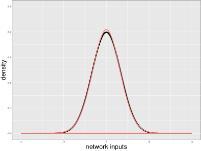
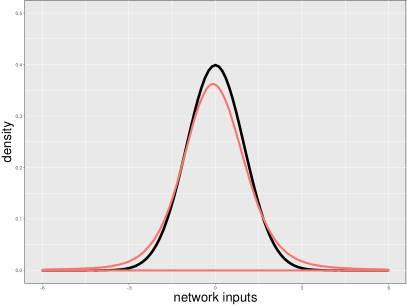
A4.4 HTRU2 data set: Hyperparameters
For the HTRU2 data set, the best hyperparameter setting was determined by a grid-search over all hyperparameter combinations using one of the 9 non-testing folds as validation fold in a nested cross-validation procedure. Concretely, if was the testing fold, we used as validation fold, and for we used fold for validation. The early stopping parameter was determined on the smoothed learning curves of 100 epochs of the validation set. Smoothing was done using moving averages of 10 consecutive values. We tested “rectangular” and “conic” layers – rectangular layers have constant number of hidden units in each layer, conic layers start with the given number of hidden units in the first layer and then decrease the number of hidden units to the size of the output layer according to the geometric progession. All methods had the chance to adjust their hyperparameters to the data set at hand.
| Hyperparameter | Considered values |
|---|---|
| Number of hidden units | {256, 512, 1024} |
| Number of hidden layers | {2, 4, 8, 16, 32} |
| Learning rate | {0.1, 0.01, 1} |
| Dropout rate | { 0, 0.05} |
| Layer form | {rectangular, conic} |
| Hyperparameter | Considered values |
|---|---|
| Number of hidden units | {256, 512, 1024} |
| Number of hidden layers | {2, 4, 8, 16, 32} |
| Learning rate | {0.1, 0.01, 1} |
| Dropout rate | {0, 0.5} |
| Layer form | {rectangular, conic} |
| Hyperparameter | Considered values |
|---|---|
| Number of hidden units | {256, 512, 1024} |
| Number of hidden layers | {2, 4, 8, 16, 32} |
| Learning rate | {0.1, 0.01, 1} |
| Normalization | {Batchnorm} |
| Layer form | {rectangular, conic} |
| Hyperparameter | Considered values |
|---|---|
| Number of hidden units | {256, 512, 1024} |
| Number of hidden layers | {2, 4, 8, 16, 32} |
| Learning rate | {0.1, 0.01, 1} |
| Normalization | {Weightnorm} |
| Layer form | {rectangular, conic} |
| Hyperparameter | Considered values |
|---|---|
| Number of hidden units | {256, 512, 1024} |
| Number of hidden layers | {2, 4, 8, 16, 32} |
| Learning rate | {0.1, 0.01, 1} |
| Normalization | {Layernorm} |
| Layer form | {rectangular, conic} |
| Hyperparameter | Considered values |
|---|---|
| Number of hidden layers | {2, 4, 8, 16, 32} |
| Learning rate | {0.1, 0.01, 1} |
| Dropout rate | {0, 0.5} |
| Hyperparameter | Considered values |
|---|---|
| Number of hidden units | {256, 512, 1024} |
| Number of residual blocks | {2, 3, 4, 8, 16} |
| Learning rate | {0.1, 0.01, 1} |
| Block form | {rectangular, diavolo} |
| Bottleneck | {0.25, 0.5} |
A5 Other fixed points
A similar analysis with corresponding function domains can be performed for other fixed points, for example for and , which leads to a SELU activation function with parameters and .
A6 Bounds determined by numerical methods
In this section we report bounds on previously discussed expressions as determined by numerical methods (min and max have been computed).
| (335) | ||||
| (336) | ||||
A7 References
References
- Abramowitz and Stegun, [1964] Abramowitz, M. and Stegun, I. (1964). Handbook of Mathematical Functions, volume 55 of Applied Mathematics Series. National Bureau of Standards, 10th edition.
- Ba et al., [2016] Ba, J. L., Kiros, J. R., and Hinton, G. (2016). Layer normalization. arXiv preprint arXiv:1607.06450.
- Bengio, [2013] Bengio, Y. (2013). Deep learning of representations: Looking forward. In Proceedings of the First International Conference on Statistical Language and Speech Processing, pages 1–37, Berlin, Heidelberg.
- Blinn, [1996] Blinn, J. (1996). Consider the lowly 22 matrix. IEEE Computer Graphics and Applications, pages 82–88.
- Bradley, [1981] Bradley, R. C. (1981). Central limit theorems under weak dependence. Journal of Multivariate Analysis, 11(1):1–16.
- Cireşan and Meier, [2015] Cireşan, D. and Meier, U. (2015). Multi-column deep neural networks for offline handwritten chinese character classification. In 2015 International Joint Conference on Neural Networks (IJCNN), pages 1–6. IEEE.
- Clevert et al., [2015] Clevert, D.-A., Unterthiner, T., and Hochreiter, S. (2015). Fast and accurate deep network learning by exponential linear units (ELUs). 5th International Conference on Learning Representations, arXiv:1511.07289.
- Dugan et al., [2016] Dugan, P., Clark, C., LeCun, Y., and Van Parijs, S. (2016). Phase 4: Dcl system using deep learning approaches for land-based or ship-based real-time recognition and localization of marine mammals-distributed processing and big data applications. arXiv preprint arXiv:1605.00982.
- Esteva et al., [2017] Esteva, A., Kuprel, B., Novoa, R., Ko, J., Swetter, S., Blau, H., and Thrun, S. (2017). Dermatologist-level classification of skin cancer with deep neural networks. Nature, 542(7639):115–118.
- Fernández-Delgado et al., [2014] Fernández-Delgado, M., Cernadas, E., Barro, S., and Amorim, D. (2014). Do we need hundreds of classifiers to solve real world classification problems. Journal of Machine Learning Research, 15(1):3133–3181.
- Goldberg, [1991] Goldberg, D. (1991). What every computer scientist should know about floating-point arithmetic. ACM Comput. Surv., 223(1):5–48.
- Graves et al., [2013] Graves, A., Mohamed, A., and Hinton, G. (2013). Speech recognition with deep recurrent neural networks. In IEEE International conference on acoustics, speech and signal processing (ICASSP), pages 6645–6649.
- Graves and Schmidhuber, [2009] Graves, A. and Schmidhuber, J. (2009). Offline handwriting recognition with multidimensional recurrent neural networks. In Advances in neural information processing systems, pages 545–552.
- Gulshan et al., [2016] Gulshan, V., Peng, L., Coram, M., Stumpe, M. C., Wu, D., Narayanaswamy, A., Venugopalan, S., Widner, K., Madams, T., Cuadros, J., et al. (2016). Development and validation of a deep learning algorithm for detection of diabetic retinopathy in retinal fundus photographs. JAMA, 316(22):2402–2410.
- Harrison, [1999] Harrison, J. (1999). A machine-checked theory of floating point arithmetic. In Bertot, Y., Dowek, G., Hirschowitz, A., Paulin, C., and Théry, L., editors, Theorem Proving in Higher Order Logics: 12th International Conference, TPHOLs’99, volume 1690 of Lecture Notes in Computer Science, pages 113–130. Springer-Verlag.
- [16] He, K., Zhang, X., Ren, S., and Sun, J. (2015a). Deep residual learning for image recognition. In IEEE Conference on Computer Vision and Pattern Recognition (CVPR).
- [17] He, K., Zhang, X., Ren, S., and Sun, J. (2015b). Delving deep into rectifiers: Surpassing human-level performance on imagenet classification. In Proceedings of the IEEE International Conference on Computer Vision (ICCV), pages 1026–1034.
- Hochreiter and Schmidhuber, [1997] Hochreiter, S. and Schmidhuber, J. (1997). Long short-term memory. Neural Computation, 9(8):1735–1780.
- Huval et al., [2015] Huval, B., Wang, T., Tandon, S., et al. (2015). An empirical evaluation of deep learning on highway driving. arXiv preprint arXiv:1504.01716.
- Ioffe and Szegedy, [2015] Ioffe, S. and Szegedy, C. (2015). Batch normalization: Accelerating deep network training by reducing internal covariate shift. In Proceedings of The 32nd International Conference on Machine Learning, pages 448–456.
- Kahan, [2004] Kahan, W. (2004). A logarithm too clever by half. Technical report, University of California, Berkeley.
- Korolev and Shevtsova, [2012] Korolev, V. and Shevtsova, I. (2012). An improvement of the Berry–Esseen inequality with applications to Poisson and mixed Poisson random sums. Scandinavian Actuarial Journal, 2012(2):81–105.
- Krizhevsky et al., [2012] Krizhevsky, A., Sutskever, I., and Hinton, G. (2012). Imagenet classification with deep convolutional neural networks. In Advances in Neural Information Processing Systems, pages 1097–1105.
- LeCun and Bengio, [1995] LeCun, Y. and Bengio, Y. (1995). Convolutional networks for images, speech, and time series. The handbook of brain theory and neural networks, 3361(10):1995.
- LeCun et al., [2015] LeCun, Y., Bengio, Y., and Hinton, G. (2015). Deep learning. Nature, 521(7553):436–444.
- Loosemore et al., [2016] Loosemore, S., Stallman, R. M., McGrath, R., Oram, A., and Drepper, U. (2016). The GNU C Library: Application Fundamentals. GNU Press, Free Software Foundation, 51 Franklin St, Fifth Floor, Boston, MA 02110-1301, USA, 2.24 edition.
- Lyon et al., [2016] Lyon, R., Stappers, B., Cooper, S., Brooke, J., and Knowles, J. (2016). Fifty years of pulsar candidate selection: From simple filters to a new principled real-time classification approach. Monthly Notices of the Royal Astronomical Society, 459(1):1104–1123.
- Mayr et al., [2016] Mayr, A., Klambauer, G., Unterthiner, T., and Hochreiter, S. (2016). DeepTox: Toxicity prediction using deep learning. Frontiers in Environmental Science, 3:80.
- Muller, [2005] Muller, J.-M. (2005). On the definition of ulp. Technical Report Research report RR2005-09, Laboratoire de l’Informatique du Parallélisme.
- Ren and MacKenzie, [2007] Ren, C. and MacKenzie, A. R. (2007). Closed-form approximations to the error and complementary error functions and their applications in atmospheric science. Atmos. Sci. Let., pages 70–73.
- Sak et al., [2015] Sak, H., Senior, A., Rao, K., and Beaufays, F. (2015). Fast and accurate recurrent neural network acoustic models for speech recognition. arXiv preprint arXiv:1507.06947.
- Salimans and Kingma, [2016] Salimans, T. and Kingma, D. P. (2016). Weight normalization: A simple reparameterization to accelerate training of deep neural networks. In Advances in Neural Information Processing Systems, pages 901–909.
- Schmidhuber, [2015] Schmidhuber, J. (2015). Deep learning in neural networks: An overview. Neural Networks, 61:85–117.
- Silver et al., [2016] Silver, D., Huang, A., Maddison, C., et al. (2016). Mastering the game of Go with deep neural networks and tree search. Nature, 529(7587):484–489.
- Srivastava et al., [2015] Srivastava, R. K., Greff, K., and Schmidhuber, J. (2015). Training very deep networks. In Advances in Neural Information Processing Systems, pages 2377–2385.
- Sutskever et al., [2014] Sutskever, I., Vinyals, O., and Le, Q. V. (2014). Sequence to sequence learning with neural networks. In Advances in Neural Information Processing Systems, pages 3104–3112.
- Wainberg et al., [2016] Wainberg, M., Alipanahi, B., and Frey, B. J. (2016). Are random forests truly the best classifiers? Journal of Machine Learning Research, 17(110):1–5.
Brief index
- Abramowitz bounds §A3.4.6, Lemma 22
- Banach Fixed Point Theorem Theorem 4
- bounds
- central limit theorem Applicability of the central limit theorem and independence assumption.
- complementary error function
- computer-assisted proof §A3.4.5
- contracting variance §A3.4.3
- definitions Normalization and SNNs.
- domain
- dropout New Dropout Technique.
- erf §A3.4.6, §A3.4.6
- erfc §A3.4.6, §A3.4.6
- error function
- expanding variance §A3.4.4
-
experiments §A4, Experiments
- astronomy Astronomy: Prediction of pulsars in the HTRU2 dataset.
-
HTRU2 §A4.4, Astronomy: Prediction of pulsars in the HTRU2 dataset.
- hyperparameters §A4.4
- methods compared Experiments
-
Tox21 §A4.3, Drug discovery: The Tox21 challenge dataset.
- hyperparameters §A4.3, Drug discovery: The Tox21 challenge dataset.
- UCI §A4.1, 121 UCI Machine Learning Repository datasets.
- initialization Initialization.
- Jacobian §A3.4.1, §A3.4.1
-
lemmata §A3.4
- Jacobian bound §A3.4.1
-
mapping Normalization and SNNs., Deriving the Mean and Variance Mapping Function .
- definition §A1
- mapping in domain §A3.4.2
- self-normalizing neural networks Definition 1
- SELU
- Theorem 1 §A2.1, Theorem 1
-
Theorem 2 §A2.2, Theorem 2
- proof §A3.2
-
Theorem 3 §A2.3, Theorem 3
- proof §A3.3