Enhancement of Network Synchronizability via Two Oscillatory System

Abstract

The loss of synchronizability at large coupling strength is of major concern especially in the fields of secure communication and complex systems. Because theoretically, the coupling mode that can surely stabilize the chaotic/hyperchaotic synchronized state is vector coupling (using all the coordinates) which is in contrast to the practical demand of information exchange using lesser number of coordinates (commonly via a single coordinate). In the present work, we propose that if the node dynamics are given by a pair of oscillators (say, two oscillatory system TOS) rather than by a conventional way of single oscillator (say, single oscillatory system SOS), then the information exchange via a single coordinate could be sufficient to stabilize the chaotic/hyperchaotic synchronization manifold at large coupling strength. The frameworks of drive-response system and Master Stability Function (MSF) have been used to study the TOS effect by varying TOS parameters with and without feedback (feedback means quorum sensing conditions). The TOS effect has been found numerically both in the chaotic (Rössler, Chua and Lorenz) and hyperchaotic (electrical circuit) systems. However, since threshold also increases as a side effect of TOS, the extent of $\beta$ enhancement depends on the choice of oscillator model like larger for Rössler, intermediate for Chua and smaller for Lorenz.

I Introduction

Synchronization is not always an obvious emergent behavior of the interacting dynamical systems even in the case when they are identical limit cycle oscillators. For an example, $N$ identical Rössler oscillators (periodic/chaotic) coupled via a single coordinate (scalar coupling) on a ring network in the nearest neighborhood configuration exhibit desynchronization at large coupling strength heagyprl2 ; pecorapre . This desynchronization behavior (known as Short Wavelength Bifurcation SWB heagyprl2 ) arises because the minimum coupling strength (threshold) requires for the synchronization increases with the increase in number of oscillators whereas the synchronization manifold in case of scalar coupling mode, losses its stability (riddle basin behavior heagyprl1 ; pecorachaos ) as the coupling strength ($\gamma$) augments towards a critical value (overload-tolerance). Thus, the small values of overload-tolerance (say $\gamma_{dsyn}$) limit the size of a synchronizable network, e.g. the synchronized state of a ring network having $x_{1}$-coupled chaotic Rössler becomes unstable with the increase in $N$ from $18$ to $19$ at $\gamma_{dsyn}=$1.5. Moreover, since the mechanism which could increment $\gamma_{dsyn}$ has not been developed so far, the network modification methods are generally used to tackle the issue of strong coupling such as (1) adding the additional edges between the nodes deterministically (Pristine World) or/and stochastically (Small World)  barahona , (2) modifying the ring network topology to a synchronizable topology like a unidirectional tree network or a star network (a hub of Scale Free network) kurthpre ; kurthchaos ; kurthphyrep1 . Practically these modifications could be considered as the distribution of overload among the nodes and theoretically these alterations imply the minimization of eigen-ratio ($R$) of the Laplacian/coupling matrix (largest eigenvalue to the smallest nonzero eigenvalue). The concept of $R$ minimization comes from the theory of Master Stability Function (MSF) pecoraprl which says that a complex network of size $N$ is synchronizable if $R<\beta$ where $\beta=\gamma_{dsyn}/\gamma_{syn}$ ($\gamma_{syn}$ means threshold) barahona . Therefore, to study the chaotic complete synchronization behavior in the complex systems, finding the different pathways that could reduce $R$ remain a primary goal for the researchers barahona ; kurthpre ; kurthchaos ; kurthphyrep1 ; pecoraprl ; boccalettiaphyrep ; lin ; Nishikawaprl ; boccalettiaprl ; donetti ; Nishikawapre ; lu ; buldu ; Boccalettipre ; amritkar . However, modification (1) increases the coupling cost of synchronization whereas the modification (2) decreases the robustness by increasing the centralization in a network.

In summary, the primary question which has not been answered yet is “how to achieve the finitely large overload-tolerance in case of scalar coupling as similar to the vector coupling scenario (wherein all coordinates are used), i.e. maximization of $\gamma_{dsyn}$ via scalar coupling”? The importance of this question lies on the fact that getting stability by using all the coordinates is neither useful (as in case of secure communication) nor realistic (as in case of complex system). Moreover, this theoretical problem also appears in many different forms such as: is it possible to stabilize the chaotic/hyperchaotic synchronization manifold? or is it possible to make a large non-centralized chaotic/hyperchaotic synchronizable network? or is it possible to surely stabilize the chaotic/hyperchaotic sub system under local/global parameter fluctuations?, etc. The answer to this question could be considered as a possible solution to the real problems such as overload failure in the real networks like Internet system and power grid system holme ; motter , the stability issue of chaotic/hyperchaotic transmitter-receiver system in the field of secure communication pecorachaos ; pecora ; pecorapra , etc. It should be noted that since large coupling strength means infinite coupling ($\gamma=\infty$) in drive-response system pecorachaos ; pecora ; pecorapra , MSF complements the drive-response formulation by explicitly incorporating $\gamma$ dependence which results into an elegant relation between the node property ($\beta$) of a just two node system (coupled bidirectionally) with the structural property ($R$) of an arbitrary network having $N$ nodes (provided coupling matrix has zero row sum). In other words, if a system is stable in the drive-response framework then at the large coupling strength MSF shows negative values and vice-versa (discussed later).

In the present work, an attempt has been made to answer the primary question of maximization of $\gamma_{dsyn}$ via scalar coupling in case of linear interactions under small perturbations and global parameter fluctuations (each node experiences same fluctuations, i.e. identical node scenario). We argue that $\gamma_{dsyn}$ could be maximized, if the node dynamics are given by a pair of oscillators (say, two oscillatory system TOS) rather than by a conventional way of single oscillator (say, single oscillatory system SOS) as schematic shown in Fig. 1 on a ring network (i.e. a basic non-centralized network). In addition, since the stabilization of synchronization manifold happens only due to the emergence of dissipative factors via TOS (explained later by drive-response framework), to maximize $\gamma_{dsyn}$ the following two conditions should be met: 1. TOS should be in mTOS configuration as dTOS configuration behaves same as SOS (discussed later), 2. only that coordinate can be employed whose self dissipation could stabilize the unstable fixed point by adding its linear dissipative term in the autonomous system (discussed later). According to condition 2, all the three coordinates of Chua chua and Lorenz lorenz oscillators fulfill this criteria whereas only two out of the three coordinates of Rössler rossler (i.e. $x_{1}$ and $x_{2}$) and also only two out of the four coordinates of piecewise electronic hyperchaotic system pecorahyper (i.e. $x_{1}$ and $x_{2}$), satisfy this condition. However, there also exist a possibility when none of the coordinates of an oscillator model like hyperchaotic Rössler rosslerhyper , could meet the condition and hence can not be employed as the oscillatory dynamics for TOS. Furthermore, since threshold increases with the increase in number of oscillators, $\gamma_{syn}$ also increases as the side effect of mTOS along with the incrementation of $\gamma_{dsyn}$. This makes $\beta$ enhancement dependent on the choice of oscillator model like larger for Rössler, intermediate for Chua and smaller for Lorenz.

The paper is organized as follows. In Sec. II, the stability issue of scalar coupling and the theory of TOS are given in terms of MSF and drive-response frameworks along with the equations of the employed oscillator models. The stabilization via TOS for the scenarios of chaotic (Rössler, Chua and Lorenz) as well as hyperchaotic (electrical circuit) oscillators are presented in Sec. III. Finally, the paper is concluded in Sec. IV.

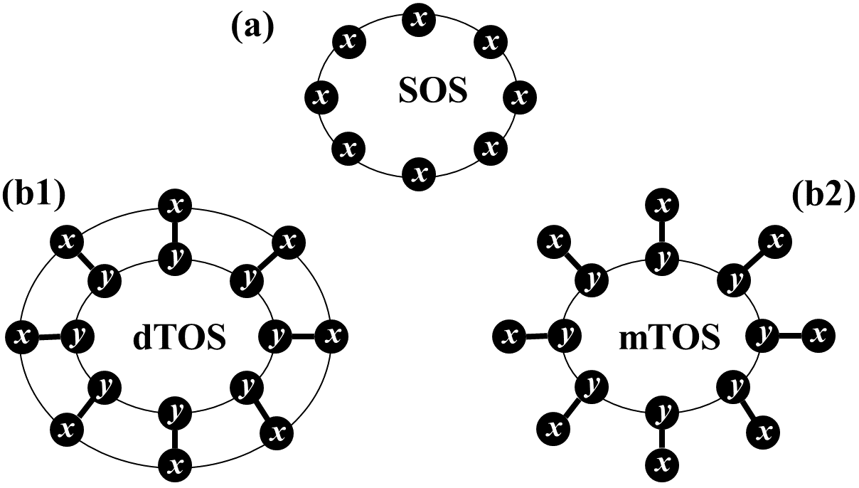
Figure 1: Schematics of a ring network (nearest neighborhood configuration bidirectionally coupled) for two scenarios: each node behaves as (a) conventional single oscillatory system (SOS), (b) proposed two oscillatory system TOS. The subplots (b1) and (b2) depict the implementation of TOS, i.e. by using both the oscillators (dTOS) and one of the oscillator (mTOS), respectively, where ‘d’ means ‘di’ and ‘m’ means ‘mono’. Oscillators $x$ and $y$ are coupled via all the coordinates (vector coupling) whereas oscillators $x$ and $x$ ($y$ and $y$) are coupled via a single coordinate (scalar coupling).

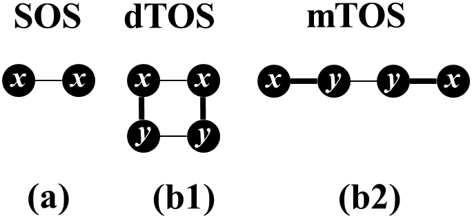
Figure 2: Schematics of a two node network (unidirectional/bidirectional) wherein oscillators $x$ and $y$ are coupled via all the coordinates (vector coupling) whereas oscillators $x$ and $x$ ($y$ and $y$) are coupled via a single coordinate (scalar coupling).

II Theory

Under small perturbations (linear analysis), Master Stability Function (MSF) serves as the necessary and sufficient condition to judge the basin stability at large coupling strength. This is analogous to the drive-response system wherein the conditional Lyapunov exponents surely determine the stability of a sub-system (response) by running the system from the different initial conditions. Therefore, the sub-Jacobian (Jacobian of response) method has been employed to investigate the reason behind the emergence of TOS effect.

II.1 MSF

To understand the formulism of MSF pecoraprl , consider the equations of motion for a complex network having $N$ identical nodes for the conventional single oscillatory system (SOS):
$\dot{x}^{i}=F(x^{i})+\gamma\sum\limits_{j=1}^{N}G_{ij}H(x^{j})$                                   (1)
Where $x^{i}$ is a $m$-dimensional vector of $i^{th}$ node whose autonomous behavior is described by $F(x^{i})$ ($R^{m}\rightarrow R^{m}$). Here, $H(x)$ ($R^{m}\rightarrow R^{m}$) represents $m\times m$ matrix (linear coupling function) which gives the information about the coordinates of $x$ involved in the coupling, i.e. its all other elements are zero except a diagonal element corresponding to the employed coordinate (for more details see ref. pecoraprl ). In Eq. 1, $G$ is a $N\times N$ coupling matrix (captures network’s architect) which could be symmetric or not but it must be real with zero row sum kurthphyrep1 so that synchronous state ($x^{i}=s$, i=1,..,N; $\dot{s}=F(s)$) could become a solution of Eq. 1. For a symmetric case (Laplacian), $G_{ii}=-g_{i}$ ($g_{i}$ is the degree/connections of $i^{th}$ node) and $G_{ij}=1$ if $i^{th}$ node is connected to $j^{th}$ node otherwise $G_{ij}=0$. The parameter $\gamma$($>0$) represents the coupling strength.

The $N$ block diagonalized linear variational equations for Eq. 1 that depict the stability of the synchronous state, i.e. evolution of perturbation ($\eta$), are pecoraprl :
$\dot{\eta}^{k}=\large(DF(s)-\gamma\delta_{k}DH(s))\eta^{k}$                                  (2)
Here $DF(s)$ and $DH(s)$ are the Jacobian matrices evaluated at $\dot{s}=F(s)$. In Eq. 2, $\delta_{k}$ ($k$=1,2,..,N) show $N$ non-negative real eigenvalues of $G$ (symmetric), such that $0=\delta_{1}\leq$$\delta_{2}\leq$..$\leq\delta_{N}$. So, the structural property becomes $R=\delta_{N}/\delta_{2}$, as $\delta_{2}$ is minimum non-zero eigenvalue ($\delta_{min}$) and $\delta_{N}$ is maximum eigenvalue ($\delta_{max}$). Now to check the network’s synchronizability, we need to evaluate node property $\beta$ from Eq. 2. For this, we proceed as follows.

Corresponding to the $N$ eigenvalues, there are $N$ maximum Lyapunov exponents, $\lambda(\gamma\delta_{k})$, wherein $\lambda(\gamma\delta_{1})$ ($\lambda(0)$ or $\lambda_{0}$) describes the state of the synchronized regime as $\lambda_{0}=0$ implies periodic and $\lambda_{0}>0$ means chaotic. The linear stability of this synchronized state is decided by the remaining $N-1$ maximum Lyapunov exponents (transverse), i.e. the given synchronous state is stable if $\lambda(\gamma\delta_{k})<0$ ($k>1$), and these $N-1$ exponents can be found from a single variational equation by using scaling relation ($\gamma\delta_{k}$) pecorapre . This means that at fixed $\gamma$, the variational equation in the presence of $\delta_{max}$ may experience stronger coupling and hence its stabilization or destabilization may occur earlier than the other modes. In other words, $\lambda(\gamma\delta_{max})$ plays a vital role in the stability condition wherein all the modes should be simultaneously stabilized or one could say that $\lambda(\gamma\delta_{max})$ can solely provides the stability of a network which is the case and hence it is called MSF for given $DF(s)$ and $DH(s)$. This is because, as long as $G$ is diagonalizable its eigenvalues corresponding to different network topologies as well as sizes can be found from any topology using scaling relation (for more details see ref. pecorachaos ; pecoraprl ). Therefore, MSF of two bidirectionally coupled nodes, i.e. $\lambda(2\gamma)$, yields same $\beta$ (=$\gamma_{dsyn}$/$\gamma_{syn}$) as an arbitrary network having $N$ nodes does,i.e. $\beta$ (=$\sigma_{dsyn}$/$\sigma_{syn}$) where $\sigma=\gamma\delta_{max}$. Now we can define $\gamma_{syn}$ and $\gamma_{dsyn}$ (similarly $\sigma_{syn}$, $\sigma_{dsyn}$), i.e. $2\gamma_{syn}$ is the minimum coupling strength at which $\lambda(2\gamma)$=$0$ or $\lambda(2\gamma)\rightarrow 0^{+}$ (emergence of synchrony) and $2\gamma_{dsyn}$ is the maximum coupling strength at which $\lambda(2\gamma)$=$0$ or $\lambda(2\gamma)\rightarrow 0^{-}$ (emergence of desynchrony).

II.1.1 Problem of scalar coupling

In contrast to the vector coupling scenario ($\lambda(\sigma\rightarrow\infty)<0$), in case of scalar coupling wherein $\lambda(\sigma)>0$ as $\sigma>\sigma_{dsyn}$ ($\sigma_{dsyn}$ is small), it becomes a challenge to synchronize a ring network topology (Fig. 1(a)) because its $R$ (i.e. $1/sin^{2}(\pi/N)$) grows faster with the increase in $N$ than any other topology, e.g. for a star network $R=N$. Therefore, the previous works on the enhancement of network’s synchronizability using network modification methods could be considered as the work on the minimization of $R=1/sin^{2}(\pi/N)$.

II.2 Drive-Response

To understand the framework of drive-response pecora ; pecorapra , consider the equations of motion for two unidirectionally coupled identical nodes for the conventional single oscillatory system SOS (Fig. 2(a)):
$\dot{x}^{1}=F(x^{1})$                                   
$\dot{x}^{2}=F(x^{2})+\gamma\Gamma(x^{1}-x^{2})$                                   (3)
Where $\Gamma$ depict same information as $H(x)$ does in Eq. 1, e.g. for $m=3$, i.e. $x$=($x_{1}$,$x_{2}$,$x_{3}$): $\Gamma$=diag(1,0,0)_3×3 or diag(0,1,0)_3×3 or diag(0,0,1)_3×3 (scalar coupling). Now we choose $x_{1}$ coordinate for the interactions and assume that the coupling term vanishes, i.e. $x^{2}_{1}\rightarrow x^{1}_{1}$, as $\gamma\rightarrow\infty$ which is only possible if $\dot{x}_{1}^{2}=\dot{x}_{1}^{1}$. This means that $x^{2}$ node instead of generating its own $x_{1}^{2}$ signal must use $x_{1}^{1}$ signal from $x^{1}$ node in order to ensure $x^{2}_{1}=x^{1}_{1}$ ($\gamma=\infty$) for all the time, i.e. even when $x^{2}_{j}\neq x^{1}_{j}$ ($j=2,..,m$). Hence, Eq. 3 becomes $\dot{x}^{2}=F(x^{2},x_{1}^{1})$ and $\dot{x}^{2}$=($\dot{x}_{2}^{2}$,..,$\dot{x}_{m}^{2}$). In this scenario, Eq. 3 depicts $x_{1}$-driving system wherein $x^{1}$ is drive and $x^{2}$ is a response sub system. The maximum conditional Lyapunov exponent ($\lambda^{c}$) of sub system (sub Jacobian) decides the stability of synchronization manifold, i.e. $\lambda^{c}<0$ implies stabilization (for more details see ref. pecorachaos ). Thus, this becomes analogous to the MSF behavior of two bidirectionally $x_{1}$-coupled nodes wherein the condition of stabilized synchronization manifold is $\lambda(2\gamma)<0$. Therefore, by using scaling relation one could also relate with the $N$ nodes scenario, i.e. $\lambda(\gamma\delta_{max})<0$ (as discussed above).

II.2.1 Problem of scalar coupling

Since the practical version of drive-response system is transmitter-receiver system in the field of secure communication, the information transfer via a single coordinate remains a primary concern. But in case of SOS, only the specific coordinates of $x$ can be used as a drive (depending upon the choice of oscillator) which sometimes can not provide the stabilization against the parameter fluctuation as the scenario of $x_{2}$-driving chaotic Rössler (shown in ref pecorapra ). Secondly, to stabilize a hyperchaotic drive-response usually a scalar signal is generated by using BK method peng which requires many parameter ($2m$). Hence, this necessitates some simpler mechanism which could work for both chaotic as well as hyperchaotic scenarios.

II.3 TOS

In contrast to SOS ($\dot{x}=F(x)$), the proposed two oscillatory system (TOS) is made up of two bidirectionally coupled oscillators (identical/nonidentical) by employing their all coordinates (vector coupling) so that the stable synchronization behavior (complete/generalized) could be ensured. Here, one should not confuse the used terminology of two oscillators with two nodes, i.e. in TOS scenario, the dynamics of a single node are generated by a pair of oscillators as:
$\dot{x}=F(x,\mu)+\gamma_{1}\Gamma_{v}(y-x)$
$\dot{y}=F(y,\mu^{\prime})+\gamma_{2}\Gamma_{v}(x-y)$
Similar to $x$, $y$ is also a $m$-dimensional vector whose autonomous behavior is described by same function $F(y)$ ($R^{m}\rightarrow R^{m}$) where $\mu$ and $\mu^{\prime}$ are the intrinsic parameters of the models. The parameters $\gamma_{1}$ and $\gamma_{2}$ represent the intra-coupling constants of TOS and $\Gamma_{v}$ shows the vector coupling scenario between $x$ and $y$, i.e. $\Gamma_{v}$$=$diag(1,..,1)_m×m. For the scenario of $\gamma_{2}$=$\theta\gamma_{1}$ (feedback), TOS could be considered as a two oscillatory representation of the quorum sensing network of $x$ oscillators interacting with each other via a $y$ oscillator (medium) singh . The parameter $\theta$ represents the population density of $x$ at each node of a network whereas $y$ may have periodic/chaotic dynamics, i.e. other than the conventional steady state behavior used in quorum sensing monte ; russo ; singh .

Further, the nodes having TOS dynamics may interact with each other in two ways, i.e. (i) each node uses either its $x$ or $y$ (mTOS, also quorum sensing type) and (ii) each node uses its both $x$ and $y$ (dTOS), as shown in Fig. 1(b) and Fig. 2(b). It has been found that only former way (mTOS) could lead to TOS effect since the latter way (dTOS) behaves same as SOS (found analytically as well as numerically). Moreover, since threshold increases with the increase in number of oscillators, $\gamma_{syn}$ also increases as the side effect of mTOS along with the maximization of $\gamma_{dsyn}$. This situation is more clear in terms of a two node network (Fig. 2) wherein SOS is the case of two oscillators (Fig. 2(a)) whereas mTOS depicts the scenario of four oscillators (Fig. 2(b2)).

To demonstrate the TOS effect in terms of MSF ($\lambda(\sigma\rightarrow\infty)<0$) and drive-response system ($\lambda^{c}<0$) for scalar coupling, we use a ring network of size $N$ (Fig. 1) and a two node network (Fig. 2), respectively. Furthermore, it should be noted that TOS could be applied to any arbitrary network topology since TOS alters only the node dynamics not the network structure, e.g. a ring network of TOS has same $R$ as for SOS, i.e. $R=1/sin^{2}(\pi/N)$ where $\delta^{ring}_{min}=4sin^{2}(\pi/N)$ and $\delta^{ring}_{max}=4$ ($N$ is even pecorapre ).

II.3.1 MSF in case of TOS

The equations of motion for the nodes of a ring network having TOS dynamics (Fig. 1(b)), are:
$\dot{x}^{i}=F(x^{i},\mu)+\gamma_{1}\Gamma_{v}(y^{i}-x^{i})$
      $+\text{\boldmath$\gamma$}{\bf\Gamma(x^{i-1}-2x^{i}+x^{i+1})}$
$\dot{y}^{i}=F(y^{i},\mu^{\prime})+\gamma_{2}\Gamma_{v}(x^{i}-y^{i})$                               (4)
      $+\text{\boldmath$\gamma$}{\bf\Gamma(y^{i-1}-2y^{i}+y^{i+1})}$
 
$\dot{x}^{i}=F(x^{i},\mu)+\gamma_{1}\Gamma_{v}(y^{i}-x^{i})$
$\dot{y}^{i}=F(y^{i},\mu^{\prime})+\gamma_{2}\Gamma_{v}(x^{i}-y^{i})$                               (5)
      $+\text{\boldmath$\gamma$}{\bf\Gamma(y^{i-1}-2y^{i}+y^{i+1})}$
Corresponding to Fig. 1(b1) and (b2), Eq. 4 and Eq. 5 respectively, represent the scenarios of N identical diffusively coupled dTOS and mTOS. The bold terms of Eq. 4-5 show the nearest neighborhood interactions form of $\gamma\sum\limits_{j=1}^{N}G_{ij}H(x^{j})$ (Eq. 1) wherein $\Gamma$ represents scalar coupling scenario (same as Eq. 3).

To understand the different behavior of dTOS and mTOS, consider the block diagonalized linear variational equations of Eq. 4-5 by using technique of spatial Fourier modes (given in ref. heagypre ):
$\dot{\eta}_{x}^{k}=(DF(s,\mu)-\gamma_{1}\Gamma_{v}{\bf-4}\text{\boldmath$\gamma$}{\bf sin^{2}(\pi k/N)\Gamma})\eta_{x}^{k}\newline \hskip 17.07182pt+\gamma_{1}\Gamma_{v}\eta_{y}^{k}$
$\dot{\eta}_{y}^{k}=(DF(y_{s},\mu^{\prime})-\gamma_{2}\Gamma_{v}{\bf-4}\text{\boldmath$\gamma$}{\bf sin^{2}(\pi k/N)\Gamma})\eta_{y}^{k}\newline \hskip 17.07182pt+\gamma_{2}\Gamma_{v}\eta_{x}^{k}$                                                   (6)
 
$\dot{\eta}_{x}^{k}=(DF(s,\mu)-\gamma_{1}\Gamma_{v})\eta_{x}^{k}+\gamma_{1}\Gamma_{v}\eta_{y}^{k}$
$\dot{\eta}_{y}^{k}=(DF(y_{s},\mu^{\prime})-\gamma_{2}\Gamma_{v}{\bf-4}\text{\boldmath$\gamma$}{\bf sin^{2}(\pi k/N)\Gamma})\eta_{y}^{k}\newline \hskip 17.07182pt+\gamma_{2}\Gamma_{v}\eta_{x}^{k}$                                                   (7)
Where $\eta_{x}^{k}=(1/N)\sum\limits_{j=0}^{N-1}\xi_{x}^{j}e^{2\pi ijk/N}$, $\eta_{y}^{k}=(1/N)\sum\limits_{j=0}^{N-1}\xi_{y}^{j}e^{2\pi ijk/N}$ and $\xi_{x}^{i}=x^{i}-s$, $\xi_{y}^{i}=y^{i}-y_{s}$. Moreover, $DF(s,\mu)$ and $DF(y_{s},\mu^{\prime})$ are the Jacobian matrices evaluated at the synchronization manifold: $x=s$, $y=y_{s}$; $\dot{s}=F(s,\mu)+\gamma_{1}\Gamma_{v}(y_{s}-s)$, $\dot{y_{s}}=F(y_{s},\mu^{\prime})+\gamma_{2}\Gamma_{v}(s-y_{s})$. The bold terms of Eq. 6-7 depict the form of $\gamma\delta_{k}DH(s)$ (Eq. 2) in case of ring network topology. Eq. 6 and 7 are corresponding to Eq. 4 (dTOS) and 5 (mTOS), respectively. By using $\eta^{\prime k}=\gamma_{2}\eta_{x}^{k}+\gamma_{1}\eta_{y}^{k}$, Eq. 6 and Eq. 7 become:
$\dot{\eta}^{\prime k}=DF(s,\mu)\gamma_{2}\eta_{x}^{k}+DF(y_{s},\mu^{\prime})\gamma_{1}\eta_{y}^{k}\newline \hskip 17.07182pt{\bf-4}\text{\boldmath$\gamma$}{\bf sin^{2}(\pi k/N)\Gamma}\eta^{\prime k}$                                     (8)
 
$\dot{\eta}^{\prime k}=DF(s,\mu)\gamma_{2}\eta_{x}^{k}+DF(y_{s},\mu^{\prime})\gamma_{1}\eta_{y}^{k}\newline \hskip 17.07182pt{\bf-4}\text{\boldmath$\gamma$}{\bf sin^{2}(\pi k/N)\Gamma}\eta^{\prime k}+\gamma_{2}{\bf 4}\text{\boldmath$\gamma$}{\bf sin^{2}(\pi k/N)\Gamma}\eta_{x}^{k}$
$\dot{\eta}_{x}^{k}=(DF(s,\mu)-(\gamma_{1}+\gamma_{2})\Gamma_{v})\eta_{x}^{k}+\Gamma_{v}\eta^{\prime k}$                  (9)
To simplify, we assume $DF(s,\mu)\approx DF(y_{s},\mu^{\prime})=D$ since TOS due to vector coupling ($\Gamma_{v}$) and strong values of intra-coupling constants ($\gamma_{1}$,$\gamma_{2}$), could behave as a system whose divergence rates from the synchronization manifold (complete/generalized) for both the oscillators could be equal even when $\delta\mu\neq 0$ ($\delta\mu=\mu^{\prime}-\mu$). This assumption is valid for every oscillator model for a given range of $\delta\mu$ (similar type of assumption had also been used previously pecorapar ). Therefore using this assumption, Eq. 8 (dTOS) becomes:
$\dot{\eta}^{\prime k}=(D{\bf-4}\text{\boldmath$\gamma$}{\bf sin^{2}(\pi k/N)\Gamma})\eta^{\prime k}$                             (10)
and Eq. 9 (mTOS) becomes:
$\dot{\eta}^{\prime k}=(D{\bf-4}\text{\boldmath$\gamma$}{\bf sin^{2}(\pi k/N)\Gamma})\eta^{\prime k}\newline \hskip 17.07182pt+\gamma_{2}{\bf 4}\text{\boldmath$\gamma$}{\bf sin^{2}(\pi k/N)\Gamma}\eta_{x}^{k}$                               (11a)
$\dot{\eta}_{x}^{k}=(D-(\gamma_{1}+\gamma_{2})\Gamma_{v})\eta_{x}^{k}+\Gamma_{v}\eta^{\prime k}$                          (11b)
The form of Eq. 10 evidently shows that dTOS behaves same as SOS (Eq. 2). On the contrary, Eq. 11 depicts that in case of mTOS, the perturbation $\eta$ also depends upon its $x$-component ($\eta_{x}$) in addition to coupling strength ($\gamma$) and eigenmodes ($k$). Moreover, since the evolution of $\eta_{x}$ does not depend on $\gamma$ and $k$ (Eq. 11b), it could act as a stability factor. However, this analysis (without numerics) does not provide any hint that $\gamma$-independent Eq. 11b could lead to the maximization of $\gamma_{dsyn}$. Thus, we need to further investigate by using drive-response framework.

Furthermore, it should be noted that since each $k$ is twice degenerate in case of ring network, MSF ($\lambda(\gamma\delta_{max})$) is obtained by solving the perturbation equations (Eq. 10-11) for $k=N/2$ (maximum eigenvalue), i.e. $\lambda(4\gamma)=\lambda(\gamma\delta_{max})$.

II.3.2 Drive-Response in case of TOS

The equations of motion for two unidirectionally coupled identical nodes having TOS dynamics are: $\dot{x}^{1}=F(x^{1},\mu)+\gamma_{1}\Gamma_{v}(y^{1}-x^{1})$, $\dot{y}^{1}=F(y^{1},\mu^{\prime})+\gamma_{2}\Gamma_{v}(x^{1}-y^{1})$
 
$\dot{x}^{2}=F(x^{2},\mu)+\gamma_{1}\Gamma_{v}(y^{2}-x^{2})$
      $+\text{\boldmath$\gamma$}{\bf\Gamma(x^{1}-x^{2}})$
$\dot{y}^{2}=F(y^{2},\mu^{\prime})+\gamma_{2}\Gamma_{v}(x^{2}-y^{2})$
      $+\text{\boldmath$\gamma$}{\bf\Gamma(y^{1}-y^{2}})$                                            (12)
 
$\dot{x}^{2}=F(x^{2},\mu)+\gamma_{1}\Gamma_{v}(y^{2}-x^{2})$
$\dot{y}^{2}=F(y^{2},\mu^{\prime})+\gamma_{2}\Gamma_{v}(x^{2}-y^{2})$
      $+\text{\boldmath$\gamma$}{\bf\Gamma(y^{1}-y^{2}})$                                            (13)
Similar to Eq. 3, the node $x^{1}-y^{1}$ is drive whereas the node $x^{2}-y^{2}$ is response. Eq. 12 and Eq. 13 depict the scenarios of dTOS and mTOS, respectively. Now we choose $x_{1}$, $y_{1}$ coordinates for dTOS whereas $y_{1}$ coordinate in case of mTOS for the interactions and assume that the coupling term vanishes at $\gamma\rightarrow\infty$. Hence, Eq. 12 and 13 become Eq. 14-15 and Eq. 16-17, respectively (same as discussed for Eq. 3):
$\dot{x}^{2}=F(x^{2},x^{1}_{1},\mu)+\gamma_{1}\Gamma_{v}(y^{2}-x^{2})$                         (14)
$\dot{y}^{2}=F(y^{2},y^{1}_{1},\mu^{\prime})+\gamma_{2}\Gamma_{v}(x^{2}-y^{2})$                         (15)
 
$\dot{x}^{2}=F(x^{2},y^{1}_{1},\mu)+\gamma_{1}\Gamma_{v}(y^{2}-x^{2})$                         (16)
$\dot{y}^{2}=F(y^{2},y^{1}_{1},\mu^{\prime})+\gamma_{2}\Gamma_{v}(x^{2}-y^{2})$                         (17)
Eq. 14-15 depict that for dTOS, $x^{2}$ and $y^{2}$ depend only on their respective missing components as $x^{1}_{1}$ only drives $x^{2}$ and $y^{1}_{1}$ only drives $y^{2}$ which is similar to Eq. 3. On the other hand, Eq. 16 shows that in case of mTOS both $x^{2}$ and $y^{2}$ are driven by same $y^{1}_{1}$. Now we need to analyze $y^{1}_{1}$ driving effect on $x^{2}$ (which is missing in dTOS). For this we decompose only Eq. 16 (because Eq. 17 is same as Eq. 15):
$\dot{x}_{1}^{2}=f_{1}(x^{2},\mu)+\gamma_{1}(y^{1}_{1}-x_{1}^{2})$                                  (18)
$\dot{x}_{i}^{2}=f_{i}(x^{2},\mu)+\gamma_{1}(y_{i}^{2}-x_{i}^{2})$                                  (19)
Where $i=2,..,m$. The relevance of $y^{1}_{1}$-drive would clearly emerge when one takes partial derivative of Eq. 18 w.r.t. $x_{1}^{2}$ which results into the addition of $-\gamma_{1}$ in the first element of sub-Jacobian whose counter balance term, i.e. $+\gamma_{1}$, is missing in the non diagonal element (i.e. $0$) because Eq. 17 does not have $\dot{y}_{1}^{2}$. Thus, this uncompensated $-\gamma_{1}$ becomes the source of TOS effect, i.e. $\lambda^{c}<0$ ($\lambda(\sigma\rightarrow\infty)<0$). This is in contrast to the sub-Jacobian for all other cases (Eq. 14-15, 17 and 19) wherein the negative term ($-\gamma_{1}/\gamma_{2}$) of the diagonal elements gets balanced by the positive terms ($\gamma_{1}/\gamma_{2}$) of non-diagonal elements. Therefore, we can say that Eq. 18 demonstrates the role of $\gamma$-independent Eq. 11b towards the maximization of $\gamma_{dsyn}$. In addition, Eq. 18 also explains the need of condition 2 (Sec. I), i.e. $x_{1}$ ($y_{1}$) should stabilize the unstable fixed point of $x$ ($y$) since the TOS effect emerges only due to the additional linear dissipative term ($-\gamma_{1}x_{1}$). Moreover, this also shows the relevance of $\gamma_{1}$, i.e. to induce the TOS effect $\gamma_{1_{01}}\leq\gamma_{1}\leq\gamma_{1_{02}}$ where $\gamma_{1_{01}}$ and $\gamma_{1_{02}}$ depend on the choice of oscillator model. In the present work, the lower bound $\gamma_{1_{01}}$ has been found by exploiting the quorum sensing conditions qs (the upper bound $\gamma_{1_{02}}$ has been located just by scanning the intra-coupling parameter space).

Furthermore, it should also be noted that in case of scalar coupling (like $\Gamma$=diag(1,0..,0)_m×m), the sub-Jacobian matrices sizes for Eq. 3 (SOS), Eq. 12 (dTOS) and Eq. 13 (mTOS) are: $(m-1)\times(m-1)$, $(2m-2)\times(2m-2)$ and $(2m-1)\times(2m-1)$, respectively.

II.4 Oscillator Models

II.4.1 Chaotic

Rössler oscillator rossler : $F(x,\mu)=[-x_{2}-x_{3};x_{1}+0.15x_{2};0.15+x_{3}(x_{1}-d)]^{\prime}$, $F(y,\mu^{\prime})=[-y_{2}-y_{3};y_{1}+\mu_{R}y_{2};\mu_{R}+y_{3}(y_{1}-d)]^{\prime}$ where $d$ and $\mu_{R}$ are the bifurcation parameters.

Chua oscillator chua : $F(x,\mu)=[8.5(x_{2}-x_{1}-g(x_{1}));x_{1}-x_{2}+x_{3};-14.97x_{2}]^{\prime}$ (chaotic behavior), $F(y,\mu^{\prime})=[\mu_{C}(y_{2}-y_{1}-g(y_{1}));y_{1}-y_{2}+y_{3};-14.97y_{2}]^{\prime}$ where $\mu_{C}$ is the bifurcation parameter and $g(x_{1}/y_{1})=mx_{1}/y_{1}+0.5(m_{0}-m)(abs(x_{1}/y_{1}+1)-abs(x_{1}/y_{1}-1))$ ($m$=-0.68;$m_{0}$=-1.31).

Lorenz oscillator lorenz : $F(x,\mu)=[10(x_{2}-x_{1});-x_{1}x_{3}+28x_{1}-x_{2};x_{1}x_{2}-2x_{3}]^{\prime}$ (chaotic behavior), $F(y,\mu^{\prime})=[10(y_{2}-y_{1});-y_{1}y_{3}+28y_{1}-y_{2};y_{1}y_{2}-\mu_{L}y_{3}]^{\prime}$ where $\mu_{L}$ is the bifurcation parameter.

II.4.2 Hyperchaotic

The employed four dimensional electronic system pecorahyper (piecewise linear form of hyperchaotic Rössler rosslerhyper ): $F(x,\mu)=[-0.05x_{1}-0.5x_{2}-0.62x_{3};x_{1}+0.15x_{2}+0.40x_{4};-2x_{3}+f(x_{1});-1.5x_{3}+0.18x_{4}+h(x_{4})]^{\prime}$, $F(y,\mu^{\prime})=[-0.05y_{1}-0.5y_{2}-0.62y_{3};y_{1}+0.15y_{2}+0.40y_{4};-2y_{3}+f(y_{1});-1.5y_{3}+0.18y_{4}+h(y_{4})]^{\prime}$ where $f(x_{1}/y_{1})=10(x_{1}/y_{1}-0.68)\Theta(x_{1}/y_{1}-0.68)$ and $h(x_{4}/y_{4})=-0.41(x_{4}/y_{4}-3.8)\Theta(x_{4}/y_{4}-3.8)$. Here, $\Theta(\cdot)$ is the Heaviside step function.

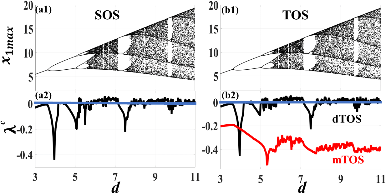
Figure 3: (Color online) For $x_{2}$-driving Rössler, plots depict the stability of two unidirectionally coupled identical nodes (Fig. 2) using $\lambda^{c}$ (a2-b2) at various dynamical regimes of Rössler (a1-b1) generated by its bifurcation parameter $d$. These plots demonstrate that the robustness emerges only for mTOS configuration, i.e. $\lambda^{c}<0$ for all $d$ values. Here, the used TOS parameters are: $\gamma_{1}$=$\gamma_{2}$=$2$ and the model parameter of $y$ is: $\mu_{R}$=$0.15$ (i.e. $y$=$x$, identical TOS scenario). Solid blue line depicts zero base line, i.e. at which $\lambda^{c}=0$.

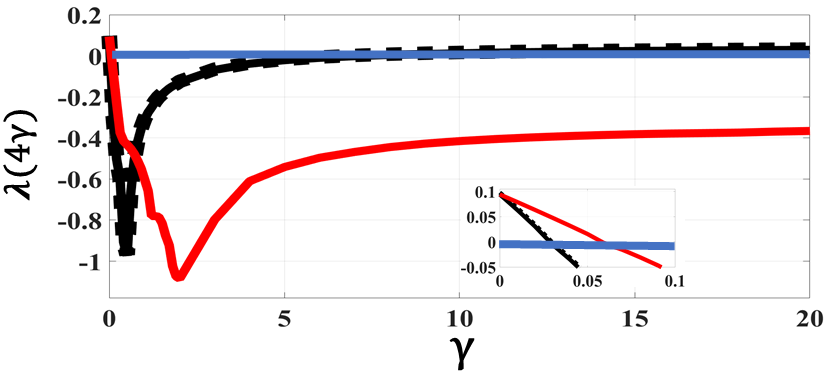
Figure 4: (Color online) Corresponding to $d=6.8$ of Fig. 3, plot depicts the stability of a ring network of $N$ identical nodes (Fig. 1) using $\lambda(4\gamma)$ (MSF) with the increase in coupling strength $\gamma$ for SOS (dotted black), dTOS (solid black) and mTOS (solid red) scenarios. Figure shows that mTOS maximizes $\gamma_{dsyn}$ whereas dTOS behaves qualitatively same as SOS, i.e. small $\gamma_{dsyn}$ (=6.01). Inset plot (magnified version) represents the behavior of MSF at small values of $\gamma$ which shows the increment of $\gamma_{syn}$ (i.e. from 0.03 to 0.06) in case of mTOS. Solid blue line depicts zero base line, i.e. at which $\lambda(4\gamma)=0$.

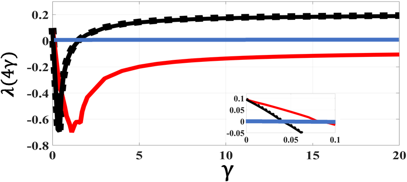
Figure 5: (Color online) For $x_{1}$-coupled chaotic Rössler, plot depicts the stability of a ring network of $N$ identical nodes (Fig. 1) using $\lambda(4\gamma)$ (MSF) with the increase in coupling strength $\gamma$ for SOS (dotted black), dTOS (solid black) and mTOS (solid red) scenarios. Figure shows that mTOS maximizes $\gamma_{dsyn}$ whereas dTOS behaves qualitatively same as SOS, i.e. small $\gamma_{dsyn}$ (=1.5). Inset plot (magnified version) represents the behavior of MSF at small values of $\gamma$ which shows the increment of $\gamma_{syn}$ (i.e. from 0.04 to 0.09) in case of mTOS. The parameters used in this scenario are same as Fig. 3-4 (i.e. identical TOS). Solid blue line depicts zero base line, i.e. at which $\lambda(4\gamma)=0$.

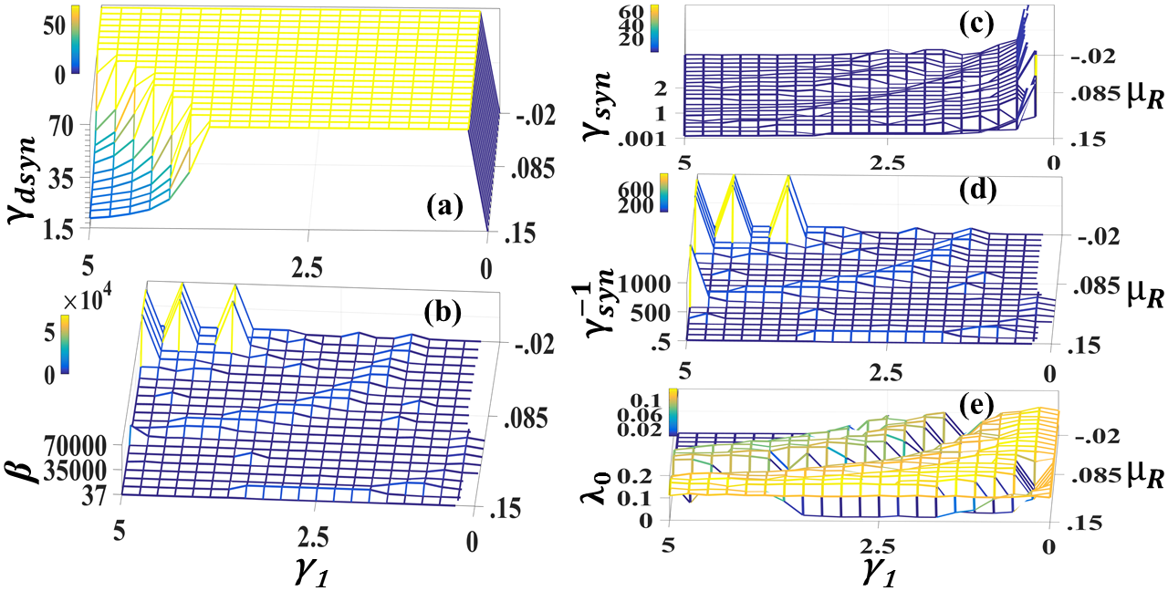
Figure 6: (Color online) Plot depicts the robustness and the side effect of mTOS in case of Fig. 5 at fixed $\gamma_{2}$=5 (no-feedback), i.e. the alterations of $\gamma_{dsyn}$ (a), $\beta$ (b), $\gamma_{syn}$ (c), $\gamma^{-1}_{syn}$ (d) and $\lambda_{0}$ tos (e) against the variation of TOS parameter $\gamma_{1}$ and the model parameter $\mu_{R}$. In subplot (a), the yellow region implies mTOS effect ($\lambda(4\gamma\rightarrow\infty)<0$), blue region shows weak-mTOS effect ($\gamma_{dsyn}>$1.5, $\lambda(4\gamma\rightarrow\infty)>0$) and no-mesh region represents no-mTOS effect ($\gamma_{dsyn}\leq$1.5, i.e. at $\gamma_{1}<\gamma_{1_{01}}$). In subplot (b), yellow region means strong-enhancement ($\beta>>$37) and blue region represents $\beta$ enhancement ($\beta>$37) where no-mesh region depicts no-enhancement ($\beta\leq$37). Subplot (c) depicts the incrementation of $\gamma_{syn}$ via mTOS (no-mesh for large $\gamma_{syn}$ as $\gamma_{1}\rightarrow 0$, $\gamma_{syn}\rightarrow\infty$). Since $\beta=\gamma_{dsyn}\gamma_{syn}^{-1}$, subplot (d) demonstrates that the enhancement as well as no-enhancement regions of subplot (b) depend on the variation of $\gamma_{syn}$. Subplots (e) and (a) show that the state of synchronization manifold $\lambda_{0}$ does not effect $\gamma_{dsyn}$.

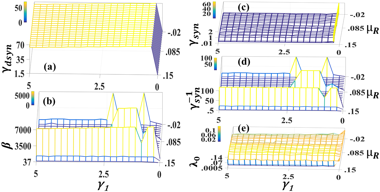
Figure 7: (Color online) Plot depicts the robustness and the side effect of mTOS in case of Fig. 5 at varying $\gamma_{2}$=5$\gamma_{1}$ (feedback), i.e. the alterations of $\gamma_{dsyn}$ (a), $\beta$ (b), $\gamma_{syn}$ (c), $\gamma^{-1}_{syn}$ (d) and $\lambda_{0}$ tos (e) against the variation of TOS parameter $\gamma_{1}$ and the model parameter $\mu_{R}$. In subplot (a), the yellow region implies mTOS effect ($\lambda(4\gamma\rightarrow\infty)<0$), blue region shows weak-mTOS effect ($\gamma_{dsyn}>$1.5, $\lambda(4\gamma\rightarrow\infty)>0$) and no-mesh region represents no-mTOS effect ($\gamma_{dsyn}\leq$1.5, i.e. at $\gamma_{1}<\gamma_{1_{01}}$). In subplot (b), yellow region means strong-enhancement ($\beta>>$37) and blue region represents $\beta$ enhancement ($\beta>$37) where no-mesh region depicts no-enhancement ($\beta\leq$37). Subplot (c) depicts the incrementation of $\gamma_{syn}$ via mTOS (no-mesh for large $\gamma_{syn}$ as $\gamma_{1}\rightarrow 0$, $\gamma_{syn}\rightarrow\infty$). Since $\beta=\gamma_{dsyn}\gamma_{syn}^{-1}$, subplot (d) demonstrates that the enhancement as well as no-enhancement regions of subplot (b) depend on the variation of $\gamma_{syn}$. Subplots (e) and (a) show that the state of synchronization manifold $\lambda_{0}$ does not effect $\gamma_{dsyn}$.

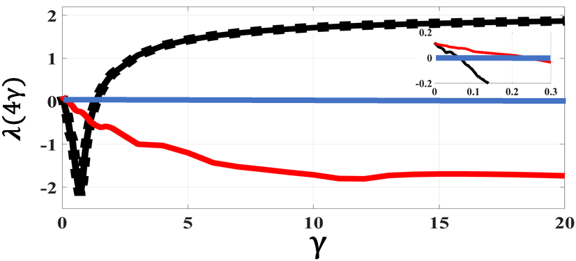
Figure 8: (Color online) For $x_{3}$-coupled chaotic Chua, plot depicts the stability of a ring network of $N$ identical nodes (Fig. 1) using $\lambda(4\gamma)$ (MSF) with the increase in coupling strength $\gamma$ for SOS (dotted black), dTOS (solid black) and mTOS (solid red) scenarios. Figure shows that mTOS maximizes $\gamma_{dsyn}$ whereas dTOS behaves qualitatively same as SOS, i.e. small $\gamma_{dsyn}$ (=1.30). Inset plot (magnified version) represents the behavior of MSF at small values of $\gamma$ which shows the increment of $\gamma_{syn}$ (i.e. from 0.09 to 0.31) in case of mTOS. Here, the used TOS parameters are: $\gamma_{1}$=2, $\gamma_{2}$=5 and the model parameter of $y$ is: $\mu_{C}$=$8.5$ (i.e. $y$=$x$, identical TOS scenario). Solid blue line depicts zero base line, i.e. at which $\lambda(4\gamma)=0$.

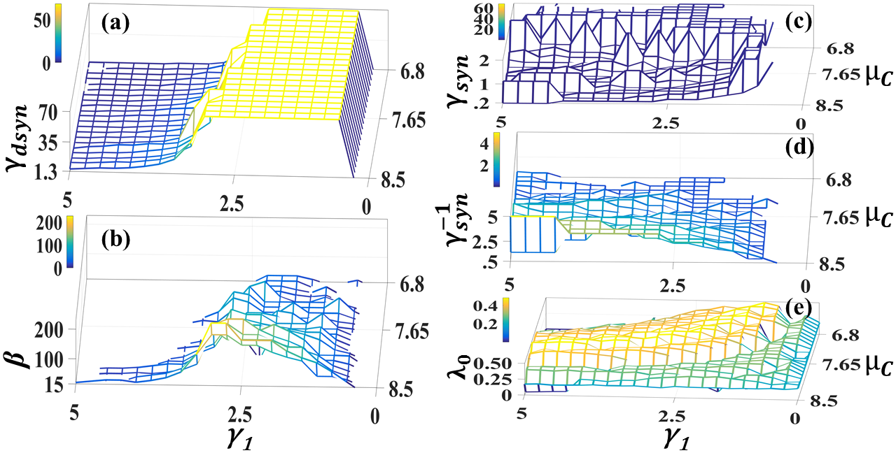
Figure 9: (Color online) Plot depicts the robustness and the side effect of mTOS in case of Fig. 8 at fixed $\gamma_{2}$=5 (no-feedback), i.e. the alterations of $\gamma_{dsyn}$ (a), $\beta$ (b), $\gamma_{syn}$ (c), $\gamma^{-1}_{syn}$ (d) and $\lambda_{0}$ tos (e) against the variation of TOS parameter $\gamma_{1}$ and the model parameter $\mu_{C}$. In subplot (a), the yellow region implies mTOS effect ($\lambda(4\gamma\rightarrow\infty)<0$), blue region shows weak-mTOS effect ($\gamma_{dsyn}>$1.3, $\lambda(4\gamma\rightarrow\infty)>0$) and no-mesh region represent no-mTOS effect ($\gamma_{dsyn}\leq 1.3$, i.e. at $\gamma_{1}<\gamma_{1_{01}}$). In subplot (b), yellow and blue regions represent $\beta$ enhancement ($\beta>$15) where no-mesh region depicts no-enhancement ($\beta\leq$15). Subplot (c) depicts the incrementation of $\gamma_{syn}$ via mTOS (no-mesh for large $\gamma_{syn}$ as $\gamma_{1}\rightarrow 0$, $\gamma_{syn}\rightarrow\infty$). Since $\beta=\gamma_{dsyn}\gamma_{syn}^{-1}$, subplot (d) demonstrates that the enhancement as well as no-enhancement regions of subplot (b) depend on the variation of $\gamma_{syn}$. Subplots (e) and (a) show that the state of synchronization manifold $\lambda_{0}$ does not effect $\gamma_{dsyn}$.

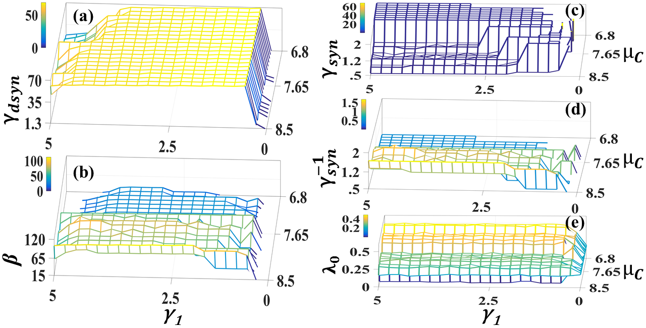
Figure 10: (Color online) Plot depicts the robustness and the side effect of mTOS in case of Fig. 8 at varying $\gamma_{2}$=5$\gamma_{1}$ (feedback), i.e. the alterations of $\gamma_{dsyn}$ (a), $\beta$ (b), $\gamma_{syn}$ (c), $\gamma^{-1}_{syn}$ (d) and $\lambda_{0}$ tos (e) against the variation of TOS parameter $\gamma_{1}$ and the model parameter $\mu_{C}$. In subplot (a), the yellow region implies mTOS effect ($\lambda(4\gamma\rightarrow\infty)<0$), blue region shows weak-mTOS effect ($\gamma_{dsyn}>$1.3, $\lambda(4\gamma\rightarrow\infty)>0$) and no-mesh region represent no-mTOS effect ($\gamma_{dsyn}\leq 1.3$, i.e. at $\gamma_{1}<\gamma_{1_{01}}$). In subplot (b), yellow and blue regions represent $\beta$ enhancement ($\beta>$15) where no-mesh region depicts no-enhancement ($\beta\leq$15). Subplot (c) depicts the incrementation of $\gamma_{syn}$ via mTOS (no-mesh for large $\gamma_{syn}$ as $\gamma_{1}\rightarrow 0$, $\gamma_{syn}\rightarrow\infty$). Since $\beta=\gamma_{dsyn}\gamma_{syn}^{-1}$, subplot (d) demonstrates that the enhancement as well as no-enhancement regions of subplot (b) depend on the variation of $\gamma_{syn}$. Subplots (e) and (a) show that the state of synchronization manifold $\lambda_{0}$ does not effect $\gamma_{dsyn}$.

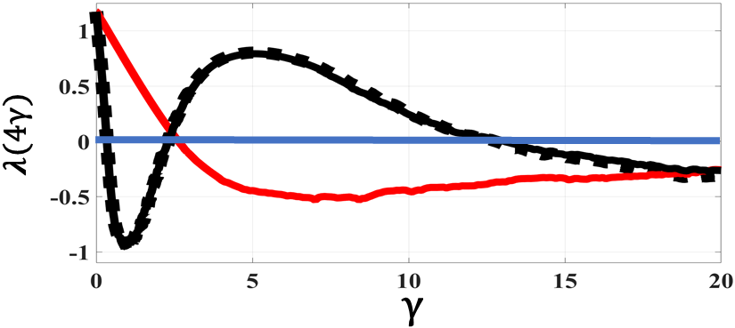
Figure 11: (Color online) For $x_{3}$-coupled chaotic Lorenz, plot depicts the stability of a ring network of $N$ identical nodes (Fig. 1) using $\lambda(4\gamma)$ (MSF) with the increase in coupling strength $\gamma$ for SOS (dotted black), dTOS (solid black) and mTOS (solid red) scenarios. Figure shows the stabilization via mTOS, i.e. the two values of $\gamma_{syn}$ (0.35 and 12.81) in the cases of SOS and dTOS, become a single value (=2.63) and first $\gamma_{dsyn}$ (2.4) is maximized. Here, the used TOS parameters are: $\gamma_{1}$=4, $\gamma_{2}$=20 and the model parameter of $y$ is: $\mu_{L}$=$2$ (i.e. $y$=$x$, identical TOS scenario). Solid blue line depicts zero base line, i.e. at which $\lambda(4\gamma)=0$.

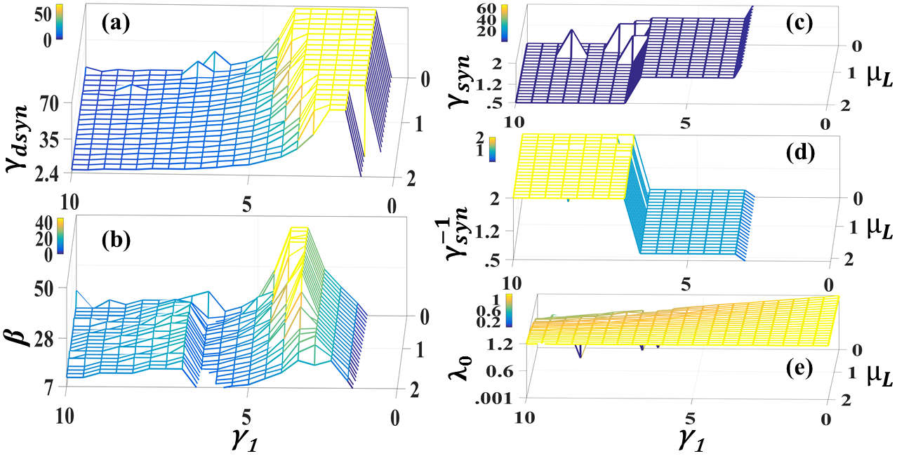
Figure 12: (Color online) Plot depicts the robustness and the side effect of mTOS in case of Fig. 11 at fixed $\gamma_{2}$=10 (no-feedback), i.e. the alterations of $\gamma_{dsyn}$ (a), $\beta$ (b), $\gamma_{syn}$ (c), $\gamma^{-1}_{syn}$ (d) and $\lambda_{0}$ tos (e) against the variation of TOS parameter $\gamma_{1}$ and the model parameter $\mu_{L}$. In subplot (a), the yellow region implies mTOS effect ($\lambda(4\gamma\rightarrow\infty)<0$), blue region shows weak-mTOS effect ($\gamma_{dsyn}>$2.4, $\lambda(4\gamma\rightarrow\infty)>0$) and no-mesh region represent no-mTOS effect ($\gamma_{dsyn}\leq 2.4$, i.e. at $\gamma_{1}<\gamma_{1_{01}}$). In subplot (b), yellow and blue regions represent $\beta$ enhancement ($\beta>$7) where no-mesh region depicts no-enhancement ($\beta\leq$7). Subplot (c) depicts the incrementation of $\gamma_{syn}$ via mTOS ((no-mesh for large $\gamma_{syn}$ as $\gamma_{1}\rightarrow 0$, $\gamma_{syn}\rightarrow\infty$). Since $\beta=\gamma_{dsyn}\gamma_{syn}^{-1}$, subplot (d) demonstrates that the enhancement as well as no-enhancement regions of subplot (b) depend on the variation of $\gamma_{syn}$. Subplots (e) and (a) show that the state of synchronization manifold $\lambda_{0}$ does not effect $\gamma_{dsyn}$.

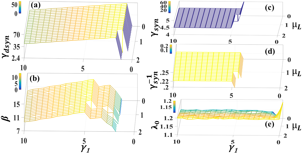
Figure 13: Plot depicts the robustness and the side effect of mTOS in case of Fig. 11 at varying $\gamma_{2}$=10$\gamma_{1}$ (feedback), i.e. the alterations of $\gamma_{dsyn}$ (a), $\beta$ (b), $\gamma_{syn}$ (c), $\gamma^{-1}_{syn}$ (d) and $\lambda_{0}$ tos (e) against the variation of TOS parameter $\gamma_{1}$ and the model parameter $\mu_{L}$. In subplot (a), the yellow region implies mTOS effect ($\lambda(4\gamma\rightarrow\infty)<0$), blue region shows weak-mTOS effect ($\gamma_{dsyn}>$2.4, $\lambda(4\gamma\rightarrow\infty)>0$) and no-mesh region represent no-mTOS effect ($\gamma_{dsyn}\leq 2.4$, i.e. at $\gamma_{1}<\gamma_{1_{01}}$). In subplot (b), yellow and blue regions represent $\beta$ enhancement ($\beta>$7) where no-mesh region depicts no-enhancement ($\beta\leq$7). Subplot (c) depicts the incrementation of $\gamma_{syn}$ via mTOS ((no-mesh for large $\gamma_{syn}$ as $\gamma_{1}\rightarrow 0$, $\gamma_{syn}\rightarrow\infty$). Since $\beta=\gamma_{dsyn}\gamma_{syn}^{-1}$, subplot (d) demonstrates that the enhancement as well as no-enhancement regions of subplot (b) depend on the variation of $\gamma_{syn}$. Subplots (e) and (a) show that the state of synchronization manifold $\lambda_{0}$ does not effect $\gamma_{dsyn}$.

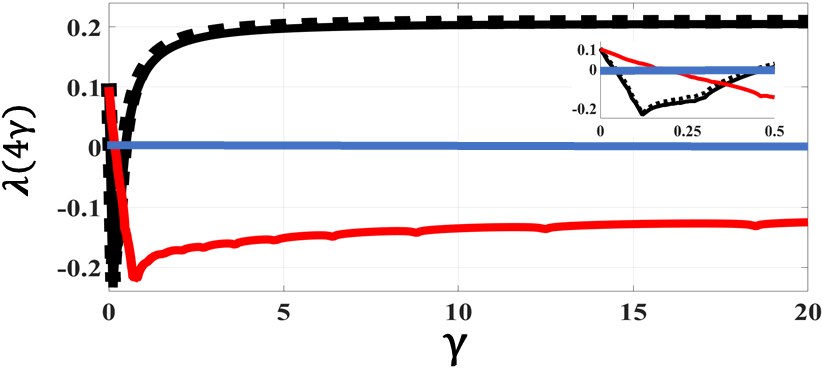
Figure 14: (Color online) For $x_{1}$-coupled hyperchaotic circuit, plot depicts the stability of a ring network of $N$ identical nodes (Fig. 1) using $\lambda(4\gamma)$ (MSF) with the increase in coupling strength $\gamma$ for SOS (dotted black), dTOS (solid black) and mTOS (solid red) scenarios. Figure shows that mTOS maximizes $\gamma_{dsyn}$ whereas dTOS behaves qualitatively same as SOS, i.e. small $\gamma_{dsyn}$ (=0.44). Inset plot (magnified version) represents the behavior of MSF at small values of $\gamma$ which shows the increment of $\gamma_{syn}$ (i.e. from 0.05 to 0.18) in case of mTOS. Here, the used TOS parameters are: $\gamma_{1}$=1, $\gamma_{2}$=3 ($y$=$x$, identical TOS scenario). Solid blue line depicts zero base line, i.e. at which $\lambda(4\gamma)=0$.

III Results and Discussions

In the present work, we employ 5 different scenarios: $x_{1}$ and $x_{2}$-coupled/driving chaotic Rössler, $x_{3}$-coupled/driving chaotic Chua, $x_{3}$-coupled/driving chaotic Lorenz and $x_{1}$-coupled/driving hyperchaotic oscillator, to generalize the TOS effect, i.e. the stabilization of chaotic/hyperchaotic synchronization manifold ($\lambda^{c}<0$) or the maximization of $\gamma_{dsyn}$ ($\lambda(4\gamma\rightarrow\infty)<0$) in case of scalar coupling. To reiterate, since these different scenarios implies different $DF$ and/or $DH$ (Eq. 2), each scenario has its own MSF. In addition, ‘coupled’ term depicts explicit $\gamma$ dependence, i.e. the stability is shown by MSF using $\lambda(4\gamma)$ (ring network) whereas ‘driving’ term shows the drive-response framework wherein the stabilization is given by maximum conditional Lyapunov exponent $\lambda^{c}$ of sub-Jacobian. Furthermore, the robustness of TOS effect has also been shown by varying the TOS parameters ($\gamma_{1}$, $\gamma_{2}$) and the model parameters of Rössler ($\mu_{R}$), Chua ($\mu_{C}$) and Lorenz ($\mu_{L}$). It has been found that the intra-coupling feedback situation (discussed in Sec. IIC) of the TOS parameters provides more robustness but lesser $\beta$ enhancement, in comparison to no feedback situation.

It should be noted that the Lyapunov exponents are calculated by using Wolf’s algorithm wolf and the model equations are integrated by using fourth order Runge-Kutta algorithm (integration step-size=0.01).

III.1 Rössler

The emergent effect of TOS for Rössler dynamics is given in Fig. 3-7 wherein Fig. 3 depicts the stabilization of $x_{2}$-driving Rössler using $\lambda^{c}$ against the variation of its bifurcation parameter $d$ for both SOS and TOS configurations. Fig. 3(a) shows the scenario (which had also been previously reported in figure 10 of ref pecorapra ) wherein the subsystem ($x_{2}$-driven Rössler) loses its stability close to the bifurcation points especially at the periodic windows in case of SOS. In contrast to Fig. 3(a), Fig. 3(b) evidently demonstrates that the mTOS configuration stabilizes the subsystem at all the domains whereas the dTOS configuration exhibits qualitatively similar behavior as of SOS (consistent with the theory). Moreover, Fig. 4 shows the MSF behavior for $x_{2}$-coupled chaotic Rössler (for SOS and TOS) corresponding to $d=6.8$ (chaos) of Fig. 3 at which synchronization manifold is stable for mTOS ($\lambda^{c}<0$) and unstable for SOS ($\lambda^{c}>0$). Now it is evident from Fig. 4 that $\lambda(4\gamma\rightarrow\infty)<0$ only happens for mTOS configuration (where ‘$\infty$’ means finitely large value). This also proves that at the large coupling strength MSF exhibits same information as the corresponding drive-response system does, i.e. $\lambda(4\gamma\rightarrow\infty)\approx\lambda^{c}$. Analogous to Fig. 4, MSF behavior shown in Fig. 5 for $x_{1}$-coupled chaotic Rössler also illustrates that only mTOS stabilizes the chaotic synchronization manifold or maximizes $\gamma_{dsyn}$. Moreover, the insets of Fig. 4 and 5 show the incrementation of $\gamma_{syn}$ as the side effect of mTOS configuration.

Furthermore, the mTOS effect shown in Fig. 5 is studied under parameter fluctuations, i.e. by varying TOS’s critical parameter $\gamma_{1}$ (discussed in Sec. IIC2) and the model parameter $\mu_{R}$ (nonidentical TOS), for no-feedback (Fig. 6) and feedback (Fig. 7) scenarios. In contrast to Fig. 6(a) wherein weak-mTOS effect observed at both small and large values of $\gamma_{1}$, Fig. 7(a) evidently demonstrates the robustness of mTOS effect ($\lambda(4\gamma\rightarrow\infty)<0$) over the broader range of parameter space in case of feedback scenario. Moreover, it also suggests that for the induction of mTOS effect at large $\gamma_{1}$, $\gamma_{1}$ should be less than $\gamma_{2}$ (one can say that the upper bound of $\gamma_{1}$, $\gamma_{1_{02}}$, also depends on $\gamma_{2}$ along with the model parameters). However, the behavior of incrementation of $\gamma_{syn}$ increases with the increase in $\gamma_{2}$ which reduces $\beta$ enhancement as depicted by Fig. 7(b)-(d) in comparison to Fig. 6(b)-(d) wherein $\gamma_{2}$ is fixed. Moreover, it should be noted that the extra strong-enhancement observed only in no-feedback scenario (Fig. 6(b)) is the consequence of decrement of $\gamma_{syn}$ due to the stable periodic synchronization manifold, $\lambda_{0}=0$ (Fig. 6(e)), which emerge at $\gamma_{1}\rightarrow\gamma_{2}$ for $\mu_{R}<0$ (Rössler’s steady state domain). But this behavior is missing in case of feedback scenario (Fig. 7(b)) because $\gamma_{2}$ increases with the increase in $\gamma_{1}$ which results into chaotic dynamics, $\lambda_{0}>0$ (Fig. 7(e)), even at $\mu_{R}<0$.

Furthermore, it is worth noticing that analogous to Fig. 3(b), the independence of $\gamma_{dsyn}$ maximization (Fig. 6(a)-7(a)) from the state of synchronization manifold (Fig. 6(e)-7(e)) clearly depict the potency of mTOS configuration.

III.2 Chua

Analogous to Fig. 5, Fig. 8 demonstrates the mTOS effect for $x_{3}$-coupled chaotic Chua and the robustness of this effect is given in Fig. 9-10 (similar to Fig. 6-7). Here also, the feedback scenario (Fig. 10) provides more robustness but lesser $\beta$ enhancement than the case of no-feedback (Fig. 9). Moreover, by comparing Fig. 9(a) with Fig. 6(a), one could realize the dependence of $\gamma_{1_{02}}$ on the oscillator model whereas Fig. 10(a) depicts that this dependence gets reduced in the presence of feedback (similar to Fig. 7(a)). But the major difference arises due to change in oscillator model from Rössler to Chua, is the extent of $\beta$ enhancement as shown in Fig. 9(b)-10(b) which is lesser in contrast to Fig. 6(b)-7(b). This is because of more augmentation of $\gamma_{syn}$ in case of Chua (Fig. 9(c)-(d) and 10(c)-(d)) than the case of Rössler (Fig. 6(c)-(d) and 7(c)-(d)). Instead of this discrepancy, Fig. 9(a)-10(a) in conjunction with Fig. 9(e)-10(e) clearly demonstrate the independence of $\gamma_{dsyn}$ maximization from the state of synchronization manifold which is similar to the case of Rössler.

III.3 Lorenz

Similar to Rössler and Chua, the case of $x_{3}$-coupled chaotic Lorenz given in Fig. 11-13 also depict more robustness but lesser $\beta$ enhancement in case of feedback (Fig. 13) than the case of no-feedback (Fig. 12). In addition, consistent with Rössler and Chua, Fig. 12(a)-13(a) in conjunction with Fig. 12(e)-13(e), evidently demonstrate the independence of $\gamma_{dsyn}$ maximization from the state of synchronization manifold. Again the difference emerge in the extent of $\beta$ enhancement (Fig. 12(b)-13(b)) which is much smaller in contrast to Rössler because $\gamma_{syn}$ augments much more in case of Lorenz.

III.4 Hyperchaotic

Fig. 14 demonstrates the mTOS effect, $\lambda(4\gamma\rightarrow\infty)<0$, in case of $x_{1}$-coupled hyperchaotic electronic system. Moreover, it is worth noticing that since $\lambda(4\gamma\rightarrow\infty)<0$ implies $\lambda^{c}<0$ (as shown for Rössler), we can say that a hyperchaotic drive-response system could also be stabilized without employing BK method peng . Furthermore, similar to the above chaotic oscillators, in case of hyperchaotic oscillator feedback scenario yields more robustness but lesser $\beta$ enhancement than the scenario of no-feedback and the state of synchronization manifold does not effect the maximization of $\gamma_{dsyn}$ (results not shown).

IV Conclusions

In the present work, without altering the network topology and without employing multi parameter BK method (previous approaches), an effort has been made to stabilize the chaotic as well as hyperchaotic synchronization manifold at large coupling strength in case of scalar coupling, just by modifying the node dynamics from a single oscillator (SOS) to a pair of oscillators (TOS). The impact of modified node configuration for both chaotic and hyperchaotic dynamics, has been studied using Master Stability Function MSF (for a fundamental non-centralized ring network) along with the drive-response framework (for a two node network). The presented results evidently dictates the potency of TOS in mTOS configuration, i.e. maximization of $\gamma_{dsyn}$ or $\lambda(4\gamma\rightarrow\infty)<0$ or $\lambda^{c}<0$, under the broad range of parametric fluctuations. Furthermore, results also demonstrate the enhancement of $\beta$ even when the threshold ($\gamma_{syn}$) augments to large values. Therefore, we believe that the proposed TOS would play a vital role both in the fields of complex system as well as secure communication wherein the network synchronizability at large coupling strength in case of scalar coupling, remains a primary concern especially for the hyperchaotic systems.

V Acknowledgement

Author would like to thank Vandana H. Singh for her valuable suggestions to improve the manuscript presentation. Financial support (501T015013, 502T016522 and TJC23) from Saitama University Japan, is acknowledged.

References

- (1) J. F. Heagy, L. M. Pecora, and T. L. Carroll, Phys. Rev. Lett. 74, 4185 (1995).
- (2) L. M. Pecora, Phys. Rev. E. 58, 347 (1998).
- (3) J. F. Heagy, T. L. Carroll, and L. M. Pecora, Phys. Rev. Lett. 73, 3528 (1994).
- (4) L. M. Pecora, T. L. Carroll, G. A. Johnson, D. J. Mar, and J. F. Heagy, Chaos 7, 520 (1997).
- (5) M. Barahona, and L. M. Pecora, Phys. Rev. Lett. 89, 054101 (2002).
- (6) A. E. Motter, C. Zhou, and J. Kurths, Phys. Rev. E. 71, 016116 (2005).
- (7) C. Zhou, and J. Kurths, Chaos 16, 015104 (2006).
- (8) A. Arenas, A. Díaz-Guilera, J. Kurths, Y. Moreno, and C. Zhoug, Phys. Rep. 469, 93 (2008).
- (9) L. M. Pecora, and T. L. Carroll, Phys. Rev. Lett. 80, 2109 (1998).
- (10) S. Boccalettia, V. Latora, Y. Morenod, M. Chavez, and D.-U. Hwanga, Phys. Rep. 424, 175 (2006).
- (11) W. Lin, H. Fan, Y. Wang, H. Ying, and X. Wang, Phys. Rev. E. 93, 042209 (2016).
- (12) T. Nishikawa, A. E. Motter, Y.-C. Lai, and F. C. Hoppensteadt, Phys. Rev. Lett. 91, 014101 (2003).
- (13) M. Chavez, D.-U. Hwang, A. Amann, H. G. E. Hentschel, and S. Boccaletti, Phys. Rev. Lett. 94, 218701 (2005).
- (14) L. Donetti, P. I. Hurtado, and M. A. Muñoz, Phys. Rev. Lett. 95,1188701 (2005).
- (15) T. Nishikawa, and A. E. Motter, Phys. Rev. E. 73, 065106(R) (2006).
- (16) Y.-F. Lu, M. Zhao, T. Zhou, and B.-H. Wang, Phys. Rev. E. 76, 057103 (2007).
- (17) J. Aguirre, R. Sevilla-Escoboza, R. Gutiérrez, D. Papo, and J. M. Buldú, Phys. Rev. Lett. 112, 248701 (2014).
- (18) R. Sevilla-Escoboza, J. M. Buldú, A. N. Pisarchik, S. Boccaletti, and R. Gutiérrez, Phys. Rev. E. 91, 032902 (2015).
- (19) S. Acharyya, and R. E. Amritkar, Phys. Rev. E. 92, 052902 (2015).
- (20) P. Holme and B.J. Kim, Phys. Rev. E 65, 066109 (2002).
- (21) A. E. Motter, and Y.-C. Lai, Phys. Rev. E 66, 065102(R) (2002).
- (22) L. M. Pecora, and T. L. Carroll, Phys. Rev. Lett. 64, 821(1990).
- (23) L. M. Pecora, and T. L. Carroll, Phys. Rev. A. 44, 2374 (1991).
- (24) L. O. Chua, M. Komuro, and T. Matsumoto, IEEE Transactions on Circuits and Systems 33, 1072 (1986)
- (25) E.N. Lorenz, J. Atmos. SCi. 20, 130 (1983).
- (26) O. E. Rössler, Phys. Lett. 57A, 397 (1976).
- (27) G. A. Johnson, D. J. Mar, T. L. Carroll, and L. M. Pecora, Phys. Rev. Lett. 80, 3956 (1998).
- (28) O. E. Rössler, Phys. Lett. 71A, 155 (1979).
- (29) S. De Monte, F. d’Ovidio, S. Dano, and P. G. Sorensen, Proc. Natl. Acad. Sci. U.S.A. 104, 18377 (2007).
- (30) G. Russo, and J. J. E. Slotine, Phys. Rev. E. 82, 041919 (2010)
- (31) H. Singh, and P. Parmananda, Nonlinear Dynamics 80, 767 (2015).
- (32) J. H. Peng, E. J. Ding and M. Ding, Phys. Rev. Lett. 76, 904(1996).
- (33) If exhibits steady behavior then for and , , i.e. the given network should also exhibit steady state behavior monte ; russo where the magnitude of depends on the chosen model as .
- (34) J. F. Heagy, T. L. Carroll, and L. M. Pecora, Phys. Rev. E. 50, 1874 (1994).
- (35) L. M. Pecora, and T. L. Carroll, Phys. Rev. E. 44, 2374 (1991).
- (36) A. Wolf, J. B. Swift, H. L. Swinney, J. A. Vastano, Physica D 16, 285 (1985).
- (37) The Lyapunov exponent parallel to synchronization manifold, , is same for both dTOS and mTOS since for mode, dTOS and mTOS follow same equation, i.e. .