Learning the structure of Bayesian Networks via the bootstrap

Abstract

Learning the structure of dependencies among multiple random variables is a problem of considerable theoretical and practical interest. Within the context of Bayesian Networks, a practical and surprisingly successful solution to this learning problem is achieved by adopting score-functions optimisation schema, augmented with multiple restarts to avoid local optima. Yet, the conditions under which such strategies work well are poorly understood, and there are also some intrinsic limitations to learning the directionality of the interaction among the variables. Following an early intuition of Friedman and Koller, we propose to decouple the learning problem into two steps: first, we identify a partial ordering among input variables which constrains the structural learning problem, and then propose an effective bootstrap-based algorithm to simulate augmented data sets, and select the most important dependencies among the variables. By using several synthetic data sets, we show that our algorithm yields better recovery performance than the state of the art, increasing the chances of identifying a globally-optimal solution to the learning problem, and solving also well-known identifiability issues that affect the standard approach. We use our new algorithm to infer statistical dependencies between cancer driver somatic mutations detected by high-throughput genome sequencing data of multiple colorectal cancer patients. In this way, we also show how the proposed methods can shade new insights about cancer initiation, and progression.

Code: https://github.com/caravagn/Bootstrap-based-Learning

1 Introduction

Learning statistical structures from multiple joint observations is a crucial problem in statistics and data science. Bayesian Networks (BNs) provide an elegant and effective way of depicting such dependencies by using a graphical encoding of conditional independencies within a set of random variables [1]. This enables a compact and intuitive modelling framework which is both highly explanatory and predictive, and justifies the enduring popularity of BNs in many fields of application [2].

Despite the undoubtable success of BNs, identifying the graphical structure underpinning a BN from data remains a challenging problem [3]. The number of possible graphs scales super-exponentially with the number of nodes [4], effectively ruling out direct search for BNs with more than a handful of nodes. Markov equivalence, the phenomenon by which two distinct graphs can encode identical conditional independence structures [5], necessarily leads to a multimodal objective function, which can be highly problematic for maximum likelihood (ML) optimisation-based and Bayesian methods alike. In practice, reasonable performance can be achieved by greedy methods that search models by their likelihood adjusted for a complexity term [6]. For information-theoretic scoring functions, common approaches are either the Bayesian Information Criterion (BIC) by Schwarz or the Akaike Information Criterion (AIC) by Akaike [7, 8]. For Bayesian scoring functions, popular choices are the Bayesian Dirichlet likelihood-equivalence score (BDE) [9] which combines the multinomial distribution with the Dirichlet prior for discrete-valued networks, or the Bayesian Gaussian equivalent (BGE) [10], which combines the linear Gaussian distribution with the normal-Wishart prior for Gaussian-valued networks, or the K2 score (K2) [9], another particular case of the Bayesian Dirichlet score. All of these approaches select network structures by a greedy optimisation process, either through (regularised) optimisation of the joint parameter/ structure likelihood, or by optimising a collapsed likelihood where the explicit dependence on the conditional parameters is marginalised under a conjugate prior distribution. As with many non-convex optimisation problems, a schema with multiple initial conditions is often used to sample different solutions from the multi-modal fitness landscape. Nevertheless, the conditions under which they should return optimal structures are poorly understood.

This paper presents a new approach to the optimisation problem for BN structural learning. Our method relies on simulating asymptotic conditions via a bootstrap procedure [11]. By bootstrapping we can estimate the frequency of each edge in the model (i.e., a conditional dependence $x\mid y$), but cannot solve the Markov equivalence problem; to address that, we follow an early intuition of Koller and Friedman and devise a data-driven strategy (again based on bootstrap) to estimate a partial ordering on the set of nodes, effectively playing the role of an informative prior over graph structures [12, 13]. Our approach therefore decouples the tasks of restricting the search space to a suitable basin of attraction, and optimising within that basin. Extensive experimentation on simulated data sets shows that the proposed algorithm outperforms several variants of regularised scores , and an experiment on a cancer genomics application shows how the approach can lead to insightful structure discovery on real life data science problems.

2 Background

In this paper we will adopt the following notation. With $\mathbf{D}\in\mathbb{B}^{n\times m}$ we denote the input data matrix with ${n}$ variables and $m$ samples. For each row a variable $\mathbf{x}_{i}$ is associated, with ${\cal X}=\{\mathbf{x}_{1},\ldots,\mathbf{x}_{n}\}$. Domain $\mathbb{B}$ can be either continuous ($\mathbb{R}$, in which case we assume to be working with Gaussian conditionals) or discrete multivariate ($\mathbb{Z}$). We aim at computing a factorization of ${p}\left({\mathbf{x}_{1},\ldots,\mathbf{x}_{n}}\right)$ from $\mathbf{D}$. We will make use of non-parametric bootstrap techniques [11]: with $\mathbf{D}\leadsto_{k}\langle\mathbf{D}_{1},\ldots,\mathbf{D}_{k}\rangle$ we denote $k$ non-parametric bootstrap replicates $\mathbf{D}_{i}\in\mathbb{B}^{n\times m}$ of the input data $\mathbf{D}$.

We are interested in a Bayesian Network (BN, [2]) ${\sf M}=\langle E,\boldsymbol{\theta}\rangle$ over variables $\cal X$, with edges $E\subseteq{\cal X}\times{\cal X}$ and real-valued parameters $\boldsymbol{\theta}$. In our formulation $E$ must induce a direct acyclic graph (DAG) over $\cal X$, that represents factorization

$${p}\left({\mathbf{x}_{1},\ldots,\mathbf{x}_{n}}\right)=\prod_{\mathbf{x}_{i}=1}^{n}{p}\left({{\mathbf{x}_{i}}\mid{\pi_{i}}}\right)\qquad{p}\left({{\mathbf{x}_{i}}\mid{\pi_{i}}}\right)=\boldsymbol{\theta}_{\mathbf{x}_{i}\mid\pi_{i}}$$ (1)

where $\pi_{i}=\{\mathbf{x}_{j}\mid\mathbf{x}_{j}\to\mathbf{x}_{i}\in E\}$ are $\mathbf{x}_{i}$’s parents, and $\boldsymbol{\theta}_{\mathbf{x}_{i}\mid\pi(\mathbf{x}_{i})}$ is a probability density function. The BN log-likelihood of ${\sf M}$ is given by

$${\sf LL}(\mathbf{D}\mid{\sf M})=\log{p}\left({{\mathbf{D}}\mid{E,\boldsymbol{\theta}}}\right)\,.$$ (2)

The model selection task $\mathbf{D}\to_{{\sf f},\Pi}^{k}{\sf M}_{\ast}$, is to compute a BN ${\sf M}_{\ast}=\langle E_{\ast},\boldsymbol{\theta}_{\ast}\rangle$ by solving

$${\sf M}_{\ast}=\arg\max_{{\sf M}=\langle E\subseteq\Pi,\boldsymbol{\theta}\rangle}{\sf LL}(\mathbf{D}\mid{\sf M})-{\sf f}({\sf M},\mathbf{D})$$ (3)

where ${\sf f}$ is a regularization score [2] (e.g., BIC, AIC, BDE, BGE, K2, etc.); notice that in this formulation we are implicitly assuming that the graph induced by the selected edges $E\subseteq\Pi$ is acyclic, i.e., a DAG. This problem is NP-hard and, in general, one can compute a (local) optimal solution to it [3]. In our definition the search-space is constrained by $E\subseteq\Pi$. Without loss of generality, we assume ${\sf M}_{\ast}$ to be estimated by a hill-climbing procedure that starts from $k$ random initial BNs, and returns the highest scoring model. When one uses information-theoretic scoring functions, parameters are maximum-likelihood estimates (MLE) of the conditional distributions [2].

We will make use also of weighted DAGs whose definition is standard; $w_{E}(\mathbf{x}_{i}\to\mathbf{x}_{j})$ will be the weight associated to edge $\mathbf{x}_{i}\to\mathbf{x}_{j}$ in a graph with edges $E$ via function $w:E\to\mathbb{R}$.

Baseline approach.

In what follows we will aim at improving over the baseline approach, which we consider to be the ${\sf f}$-regularized selection with unconstrained search space and $k$ initial conditions

$$\mathbf{D}\to_{{\sf f},\emptyset}^{k}{\sf M}_{\ast}\,.$$

This procedure is greedy, it starts from an initial condition ${\sf M}_{0}$ – e.g., a random DAG – and performs a one-edge change (deletion or insertion of an edge) to exhaustively compute the neighbourhood ${\cal M}_{0}$ of ${\sf M}_{0}$. Then, $\hat{{\sf M}}\in{\cal M}_{0}$ is the new best solution if it has score – according to equation (3) – higher than ${\sf M}_{0}$ and is the maximum-scoring model in the whole neighbourhood. The greedy search then proceed recursively to examine $\hat{{\sf M}}$’s neighbourhood, and stops if the current solution is the highest scoring in all of its neighbourhood. Thus, this search scans a set of solutions $\{{\sf M}_{i}\}_{I}$ by maximising the discrete gradient defined as

$$\nabla_{{\sf M}_{i},\hat{{\sf M}}}=f(\hat{{\sf M}})-f({\sf M}_{i}), \hat{{\sf M}}\in{\cal M}_{i}$$ (4)

where $f({\sf M})={\sf LL}(\mathbf{D}\mid{\sf M})-{\sf f}({\sf M},\mathbf{D})$ is the scoring function in equation (3).

Hill Climbing is known to be suboptimal, and can be improved in several ways. For instance, instead of sampling $k$ uncorrelated initial conditions (random restarts), one can sample a model in the neighbourhood of the last computed solution and proceed through an iterated local search. To navigate iteratively the space of solutions one can take into account structural-equivalence classes, node orderings, and edge reversal moves; see [14, 15, 16, 17, 18] and references therein. Other approaches can guarantee exact Bayesian structure learning by applying either dynamic programming [19, 20] or integer linear programming, [21, 22] nevertheless, the number of valid solutions remains still potentially huge and Markov equivalence still poses challenges. We refer to [23, 24] for recent reviews of approches for structure learning of Bayesian Networks. For simplicity, here we consider the baseline Hill Climbing; it would be straightforward to improve our approach by adopting other search or restart strategies proposed in the literature.

In this paper we consider several common scores for BNs: the BIC, AIC, BDE, BGE and K2. In the Main Text, we discuss results obtained with the information-theoretic scores ${\sf f}\in\{{\sf BIC},{\sf AIC}\}$; ${\sf BIC}$ is derived as the infinite samples approximation to the MLE of the structure and the parameters of the model, and is consistent, while AIC is not. In the Supplementaty Material, we present that analogous results hold for Bayesian scoring functions (${\sf f}\in\{{\sf BDE}{},{\sf BGE}{},{\sf K2}\}$).

Searching for the optimal network requires also to account for the fact that different DAGs can induce the same distributions; this is formalised through the notion of $v$-structures and likelihood equivalence, which are structural properties of BNs introduced in Section 3 (together with one example). Intuitively, if we denote by $K_{\sf M}$ the set of likelihood-equivalent models, even in the case of infinite samples ($m\to+\infty$) asymptotic convergence is up to Markov equivalence. This mean, in practice, that we can at best identify one of the models in the equivalence class $K_{{\sf M}_{\sf T}}$, not necessarily the true one, and therefore the fitness landscape is multi-modal, each mode being one of the elements of $K_{{\sf M}_{\sf T}}$. For finite $m$, model-selection is even more complicated. The landscape induced by the likelihood function is rugged and there could $i)$ be structures scoring higher than the ones in $K_{{\sf M}_{\sf T}}$, and $ii)$ also higher than the models in their neighbourhood (thus suggesting the importance of testing also randomised restarts). Thus, such structures as well as their equivalence classes would create further optima; we present one example of this models in Section 3, and a portrait the associated multi-modal landscape in Figure 2. For this reason, besides the problem of identifying the one true model ${\sf M}_{\sf T}$ within $K_{{\sf M}_{\sf T}}$, a greedy search is likely be trapped into local optima, and heuristics use multiple initial conditions to minimize such an effect.

3 An example

We give an intuitive introduction to the concept of fitness landscape associated with this optimisation problem, and show its computation on a real network.

Definition 3.1 (Fitness).

Consider $\mathcal{M}\subset{\cal X}\times{\cal X}$ the set of all possible non-reflexive edges over variables in set $\cal X$. For a subset $\Pi\subseteq\mathcal{M}$, let ${\cal F}_{\Pi,{\sf f}}:2^{\mathcal{M}}\mapsto\mathbb{R}^{+}$ be the fitness function of the state space $2^{\Pi}$, data $\mathbf{D}$ and regularization ${\sf f}$ and the BN ${\sf M}=\langle E,\boldsymbol{\theta}\rangle$ to be defined by

$${\cal F}_{\Pi,{\sf f}}(E)=\begin{cases}{\sf LL}(\mathbf{D}\mid{\sf M})-{\sf f}({\sf M},\mathbf{D})\,,&\text{if $E\subseteq\Pi$, $E$ acyclic,}\\ 0&\text{otherwise.}\end{cases}$$ (5)

Then, ${\cal F}_{\Pi,{\sf f}}(\cdot)$ defines the fitness landscape which we use to search for a BN model ${\sf M}^{\sf MLE}=\langle E^{\sf MLE},\boldsymbol{\theta}^{\sf MLE}\rangle$ that best explains $\mathbf{D}$ in the sense of equation (3).

So, in practice, a search that constraints the state space by $\Pi$ spans through the subspace of DAGs induced by $2^{\Pi}\subseteq 2^{\mathcal{M}}$. Let us denote the true model as the BN ${\sf M}_{\sf T}=\langle E_{\sf T},\boldsymbol{\theta}_{\sf T}\rangle$, $E_{\sf T}\in 2^{\Pi}$; for $m\to\infty$, the landscape’s MLE structure is $E_{\sf T}$, when ${\sf f}$ is a consistent estimator (${\sf BIC}$ does satisfy this property, if at least one of several models contains the true distribution [25]). Unfortunately, the MLE is not unique even for infinite sample size.

Proposition 3.2 (Likelihood equivalence [2], Figure 2).

For any BN ${\sf M}=\langle E,\boldsymbol{\theta}\rangle$ there exists $K_{\sf M}=\{{\sf M}_{i}=\langle E_{i},\boldsymbol{\theta}_{i}\rangle\}_{I}$ for some index set $I$, such that ${\cal F}_{\mathcal{M},{\sf f}}(E_{i})={\cal F}_{\mathcal{M},{\sf f}}(E_{j})$ for every ${\sf M}_{i},{\sf M}_{j}\in K_{\sf M}$.

We term $K_{\sf M}$ a Markov equivalence (or I-equivalence) class of BNs with equivalent fitness value, but different structure. Thus, we can not expect to identify ${\sf M}_{\sf T}$ among $K_{{\sf M}_{\sf T}}$’s models by looking at ${\cal F}_{\mathcal{M},{\sf f}}(\cdot)$, which leaves us with, at least, $|K_{{\sf M}_{\sf T}}|$ equivalent maxima. Such class exists due to symmetries of the likelihood function that are induced by $v$-structures.

Definition 3.3 ($v$-structure [5], Figure 2).

A triplet $(\mathbf{x}_{i},\mathbf{x}_{j},\mathbf{x}_{k})$ is a $v$-structure in a set of edges $E$ if $\mathbf{x}_{i}\to\mathbf{x}_{k},\mathbf{x}_{j}\to\mathbf{x}_{k}\in E$ but $\mathbf{x}_{i}\to\mathbf{x}_{j},\mathbf{x}_{j}\to\mathbf{x}_{i}\not\in E$.

Figure 1: Exhaustive portrait of the fitness landscape ${\cal F}$ (Definition 3.1) for a random BN with $n=4$ variables, random conditional distributions $\boldsymbol{\theta}$ and $10000$ samples. The scoring function uses BIC. Each node is a candidate BN, whose score is given by the color’s intensity (darker is better). In total, there are $543$ BNs. Each edge represents the maximum of the optimization gradient in equation (4)S, which is followed by a greedy heuristics such as Hill Climbing. Here the neighbourhood of a model is the set of models that differs by one edge. A basin of attraction is a set of initial conditions that lead to the same solution. Here the true model is associated to a mid-size basin of attraction, highlighted in top right of the plot. In Figure 2 we show the local optima, the true model and a way to re-shape ${\cal F}$.

Figure 2: The 13 optima of the fitness landscape shown in Figure 1, with their BIC score. Notice the equivalence classes (discussed in Section 3) and the presence of optima with equivalent score but different structure. The true, i.e., generative, model is not the highest ranked in ${\cal F}$. If we create as poset $\Pi$ the transitive closure of the true model, however, we observe that the landscape reduces to having a unique global optima. In fact, all the optima but the true one have at least one edge not included in $\Pi$. For this $\Pi$, the landscape happens to be unimodal with a maximum at the true model; an experiment with $100$ random networks shows that this happens with high probability.

Example with a simple network.

We begin with an example that inspired the approach that we introduce in Section 4. Let us consider a random BN ${\sf M}$ with $n=4$ discrete nodes (${\cal X}=\{\mathbf{x}_{1},\ldots,\mathbf{x}_{4}\}$, $\mathbb{B}=\{0,1\}$), $|\pi_{i}|\leq 2$, and random conditional distributions $\boldsymbol{\theta}$ (parameters). Despite being small, models of this size show a rich optimization’s landscape and allow for some visualization. In fact, the number of DAGs with $n$ nodes is super-exponential in $n$. Precisely, it is computable as

$$G(n)=\sum_{k=1}^{n}(-1)^{k+1}{n\choose k}2^{k(n-k)}G(n-k)$$

as shown in [4]; in this case leads to $G(n)=543$ models. From ${\sf M}$, we generate $m=10000$ samples and investigate the problem of identifying ${\sf M}$ from such data.

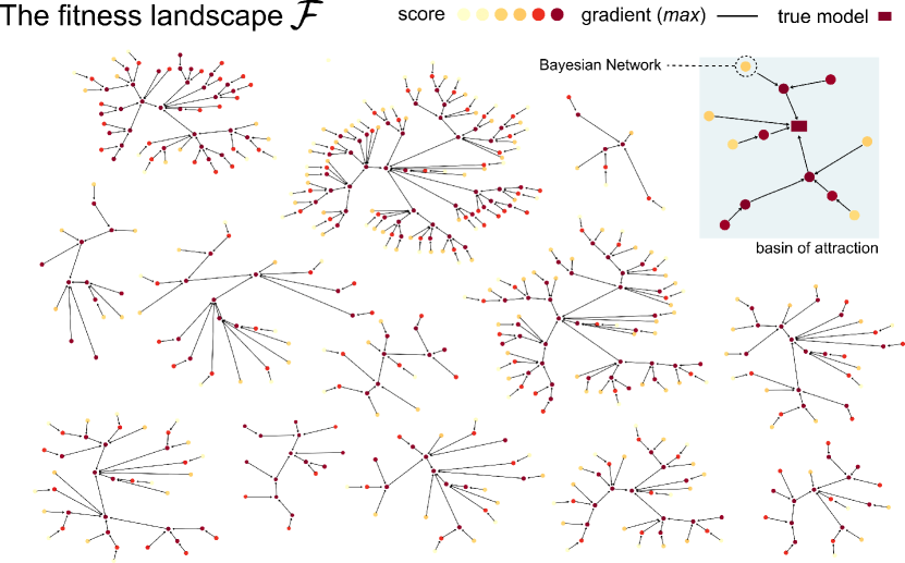
With such a small network we can exhaustively construct the fitness landscape ${\cal F}$ of the discrete optimization, and visualize the gradient in equation (4) used to solve equation (3). The whole landscape of the Hill Climbing with BIC scores is shown in Figure 1, and shows that:

• there are several models with different structure but equivalent BIC score;

• ${\sf M}$’s BIC score is not the highest in this landscape, which has 13 optima;

• the basins of attractions can be fairly large, compared to ${\sf M}$’s one;

We expect the landscape to have multiple modes because of Markov equivalence classes (Definition 3.2), and because we are working with finite $m$. Thus, a search in this landscape could likely be trapped in optima that are not ${\sf M}$.

We now focus on the intuition that searching for the model is generally easier if one constrains the parent sets [2]. This is often done by either setting a cutoff on $|\pi_{i}|$, i.e., limiting the number of $\mathbf{x}_{i}$’s parents, or by specifying a partially ordered set (poset) $\Pi\subseteq{\cal X}\times{\cal X}$ such that $\mathbf{x}_{j}$ can be one of $\mathbf{x}_{i}$’s parents only if $(\mathbf{x}_{j},\mathbf{x}_{i})\in\Pi$. Whatever the case, the algorithmic motivation seems obvious as we drop the search’s combinatorial complexity by pruning possible solutions. However, we are interested in investigating how this affects the shape of the landscape ${\cal F}$.

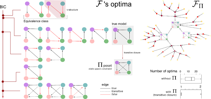
We consider the constraint to be given as a poset $\Pi$ (that, in practice, one has to estimate from data). The search is then limited to analyzing edges in $\Pi$, so $\Pi$ is good if it shrinks the search to visit solutions that are “closer” to ${\sf M}$ – thus, $\Pi$ has to include ${\sf M}$’s edges. In this example we create $\Pi$ by adding to ${\sf M}$ also its transitive edges. In Figure 2 we show that all the models (but ${\sf M}$) that are optima in ${\cal F}$ have at least one edge that is not allowed by $\Pi$. So, they would not be visited by a search constrained by this $\Pi$.

We compute the fitness landscape under $\Pi$, ${\cal F}_{\Pi}$, and find it to have a unique optimum (Figure 2). For this poset, ${\cal F}_{\Pi}$ is unimodal with a maximum at the true model. ${\sf M}$’s basin of attraction in ${\cal F}_{\Pi}$ is larger than in ${\cal F}$, as one might expect. This clearly suggests that we are also enjoying a simplification of the “statistical part” of the problem, which we observe with high probability ($98$ times out of $100$) in a sample of random networks. In two cases, we observed two optima in ${\cal F}_{\Pi}$ (${\sf M}$ and one of its subsets, data not shown). Thus, greedy optimization of equation (3) in this setting would lead to the globally optimal solution ${\sf M}$.

The above considerations are valid for the $\Pi$ derived as transitive closure of ${\sf M}$. In real cases, of course, we do not know ${\sf M}$ and cannot trivially build this $\Pi$. We can, however, try to approximate $\Pi$ from $\mathbf{D}$. In practical cases, of course, the landscape will still be multi-modal under the approximated poset, but one would hope that the number of modes is reduced and the identification of the true model made easier in the reduced search-space.

Algorithm 1 – Model selection for BNs via the bootstrap (Figure 3.)
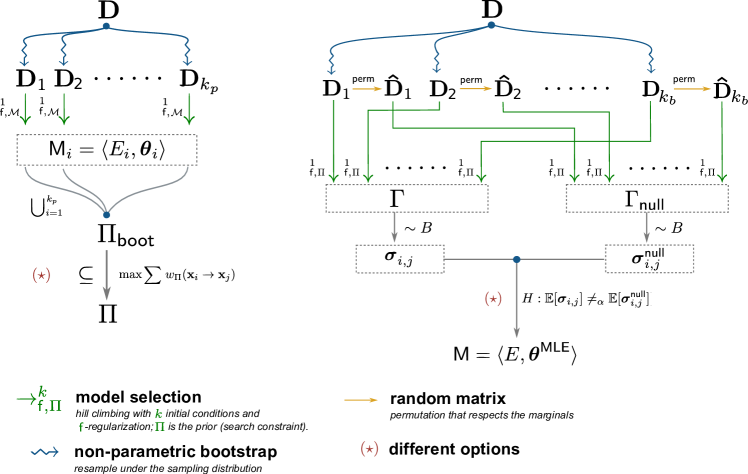
Steps marked with ($\star$) can be implemented in different ways (see Sections 4.1–4.2).

0:  a dataset $\mathbf{D}$ over variables $\cal X$, and two integers $k_{p}$, $k_{b}\gg 1$;

1:  let $\mathbf{D}\leadsto_{k_{p}}\langle\mathbf{D}_{1},\ldots,\mathbf{D}_{k_{p}}\rangle$ be $k_{b}$ bootstrap resamples from $\mathbf{D}$, and $\mathcal{M}\subset{\cal X}\times{\cal X}$ be the set of non-reflexive edges over $\cal X$.

2:  compute the weighted consensus structure $\Pi_{{\sf boot}}$

$$\Pi_{{\sf boot}} =\bigcup_{i=1}^{k_{p}}\Big{\{}E_{i}\mathrel{}|\mathrel{}\mathbf{D}_{i}\to_{{\sf f},\mathcal{M}}^{1}{\sf M}_{i}=\langle E_{i},\boldsymbol{\theta}_{i}\rangle\Big{\}} w_{\Pi_{\sf boot}}(\mathbf{x}_{i}\to\mathbf{x}_{j})=\sum_{w=1}^{k_{p}}\mathbf{1}_{E_{w}}(\mathbf{x}_{i}\to\mathbf{x}_{j})\,;$$ (6)

where by $\mathbf{D}_{i}\to_{{\sf f},\mathcal{M}}^{1}{\sf M}_{i}$ we mean to learn the BN ${\sf M}_{i}$ from the bootstrap sample $\mathbf{D}_{i}$ using a single run, ${\sf f}$-regularisation and scanning all possible edges ($\mathcal{M}$);

3:  ($\star$) remove loops from $\Pi_{{\sf boot}}$ by solving

$$\Pi=\arg\max_{\begin{subarray}{c}\Pi_{\ast}\subseteq\Pi_{\sf boot}\\ \Pi_{\ast}\text{ \sf acyclic}\end{subarray}}\quad\sum_{\mathbf{x}_{i}\to\mathbf{x}_{j}\in\Pi}w_{\Pi}(\mathbf{x}_{i}\to\mathbf{x}_{j})\,;$$ (7)

4:  let $\mathbf{D}\leadsto_{k_{b}}\langle\mathbf{D}_{1},\ldots,\mathbf{D}_{k_{b}}\rangle$, for any $\mathbf{D}_{i}$ generate $\hat{\mathbf{D}}_{i}={\sf perm}(\mathbf{D}_{i})$;

5:  compute $2k_{b}$ BNs under $\Pi$

$$\Gamma =\{{E}_{i}\mid\mathbf{D}_{i}\to_{{\sf f},\Pi}^{1}{\sf M}_{i}=\langle{E}_{i},\boldsymbol{\theta}_{i}\rangle\} \Gamma_{\sf null}=\{{E}_{i}\mid\hat{\mathbf{D}}_{i}\to_{{\sf f},\Pi}^{1}{\sf M}_{i}=\langle{E}_{i},\boldsymbol{\theta}_{i}\rangle\}\,,$$ (8)

Note that here we use $\Pi$ to constrain the search space for each BN;

6:  let $\boldsymbol{\sigma}_{i,j}=[\cdots\mathbf{1}_{x}(\mathbf{x}_{i}\to\mathbf{x}_{j})\cdots]_{x\in\Gamma}$ and $\boldsymbol{\sigma}_{i,j}^{{\sf null}}=[\cdots\mathbf{1}_{x}(\mathbf{x}_{i}\to\mathbf{x}_{j})\cdots]_{x\in\Gamma_{\sf null}}$;

7:  ($\star$) to select $\mathbf{x}_{i}\to\mathbf{x}_{j}$, test $H$ at level $\alpha$ with Multiple Hypotheses Correction (MHC) and output the Bayesian Network ${\sf M}=\langle E,\boldsymbol{\theta}^{\sf MLE}\rangle$ where

$$E =\{\mathbf{x}_{i}\to\mathbf{x}_{j}\mid H:\mathbb{E}[\boldsymbol{\sigma}_{i,j}]\neq_{\alpha}\mathbb{E}[\boldsymbol{\sigma}_{i,j}^{\sf null}]\} \theta^{{\sf MLE}{}}=\arg\max_{\boldsymbol{\theta}\in\Theta}\log{p}\left({{\mathbf{D}}\mid{E,\boldsymbol{\theta}}}\right)\,.$$ (9)

Figure 3: Graphical representation of Algorithm 1. Left: first phase (construction of the poset $\Pi$). Right: second phase (construction of the test under the poset $\Pi$).

4 Model selection for BNs via empirical Bayes

We present our method as Algorithm 1; the algorithm exploits a combination of non-parametric bootstrap estimates, likelihood-fit and hypothesis testing to infer a BN . The algorithm is conceptually divided in two phases (Figure 3) that can be customized, as we discuss in the next subsections.

Phase one: construction of the poset $\Pi$.

The first phase (steps 1–3) uses a bootstrap strategy to estimate an ordering $\Pi$ of the model’s variables; this ordering constraints the factorization in the second phase of the algorithm. The bootstrap is used in the following way. For $k_{p}$ times we sample with repetition a dataset of equal size with respect to the input dataset $\mathbf{D}$ – i.e., this is a classic non-parametric bootstrap scheme. For each bootstrap sample we run the standard model selection strategy: i.e., we denote by $\mathbf{D}_{i}\to_{{\sf f},\mathcal{M}}^{1}{\sf M}_{i}$ the learning of the model ${\sf M}_{i}$ from the bootstrap sample $\mathbf{D}_{i}$ using a single run (no restarts), ${\sf f}$-regularisation and scanning all possible edges ($\mathcal{M}$) to create the model. This steps practically creates $k_{p}$ models.

The union $\Pi_{{\sf boot}}$ of all the $k_{p}$ models’ structures is obtained by merging all the fits from the non-parametric bootstrap replicates. This is a trivial graph union operation which, of course, does not necessarily preserves the acyclic condition required by a BN. This structure is called consensus as it contains the union of all the models that are obtained by a standard regularized likelihood-fit procedure. Notice that each model is obtained from one initial condition, and without restrictions on the set of candidate edges that can populate the models. Each models’ parameters (i.e., the conditional probability tables) are dropped, and $\Pi_{{\sf boot}}$ is instead augmented with the non-parametric bootstrap scores via the set indicator function $\mathbf{1}_{X}(y)=1\iff y\in X$. This is just a way of counting how often each edge is detected across the $k_{p}$ bootstrap resamples; thus $w_{\Pi_{\sf boot}}(\cdot)$ is proportional to the edges’ frequency across the $k_{p}$ bootstrap models.

The graph induced by $\Pi_{{\sf boot}}$ is generally cyclic, and is weighted. In step 3, we render it acyclic by selecting a suitable subset of its edges: $\Pi\subseteq\Pi_{{\sf boot}}$. This loop-breaking strategy is based on the idea of maximizing the scores of the edges in $\Pi$, and is motivated by the intuition that true model edges should have higher bootstrap scores[12]. The optimization problem that determines $\Pi$, equation (7), can be solved in different ways, as we discuss in Section 4.1.

Phase two: using $\Pi$ to construct a final model.

The second phase (steps 4-7) is the actual selection of the final output model. In principle, we could just use the standard regularized likelihood-fit procedure to select a model under $\Pi$. Preliminary tests (data not shown), however, have highlighted an intrinsic bias in the selected ouput model, as a function of the regularizer ${\sf f}$. We would like to reduce to the minimal extent this effect, while enjoying the properties of ${\sf f}$ to minimize overfit. Thus, we exploit $\Pi$ to create an edge-specific statistical test to detect true edges, and create the final output model. Here, if $\Pi$ is a good approximation to the transitive closure of the true model (such as in the example of Section 3), then $\Pi$ will direct the search to get better estimates for the test; therefore in this case, an approximation is “good” if it contains all the true model edges.

The test null hypothesis $H_{0}$ is created from $\mathbf{D}$, again by exploiting a bootstrap procedure. We begin by creating (step 4) $k_{b}$ bootstrap resamples of $\mathbf{D}$, as in step one of the algorithm; from each replicate we generate a permutation matrix $\hat{\mathbf{D}}_{i}\in\mathbb{B}^{n\times m}$, with equivalent empirical marginal distributions. The construction of the matrix depends on the type of distributions that we are modelling; let $p_{i}(\mathbf{x}_{j})$ and $\hat{p}_{i}({\mathbf{x}}_{j})$ be the empirical marginals of $\mathbf{x}_{j}$ in $\mathbf{D}_{i}$ and $\hat{\mathbf{D}}_{i}$. If $\mathbf{x}_{j}$ is discrete multivariate we require $p_{i}(\mathbf{x}_{j})=\hat{p}_{i}({\mathbf{x}}_{j})$. If $\mathbf{x}_{j}$ is continuous, we require the expectation and variance to be equivalent. We achieve this with a shuffling approach: we independently permute $\mathbf{D}_{i}$’s row vectors – in the algorithm denoted by function perm$(\cdot)$. The joint distributions in each $\hat{\mathbf{D}}_{i}$ are random, so for each pair $(\mathbf{x}_{i},\mathbf{x}_{j})$ we have a null model of their statistical independence normalized for their marginal distributions. At this point we have a pair of $2k_{b}$ datasets, half of them are bootstrap resamples, and the other half are matched permutation datasets. We can now fit a model for each on of these datasets; in this case we use the same fitting strategy adopted in the first step of the algorithm, but constraining the edges to include in the mode by using the poste $\Pi$. The obtained $2k_{b}$ models are split into two groups depending on the data we used to generate them (non-permuted versus permuted); the two groups are called $\Gamma$ and $\Gamma_{\sf null}$ (the models from the null hypothesis), and the edges are counted as in the step one of the algorithm. Thus, if we fit a model on ${\mathbf{D}}_{i}$ and $\hat{\mathbf{D}}_{i}$ (step 5) we expect that an edge that represents a true dependency will tend to be more often present in $\Gamma$, rather than in $\Gamma_{\sf null}$.

Steps 6 and 7 perform multiple hypothesis testing for edges’ selection. We use the models computed in step 5 as a proxy to test for the dependencies. The vectors $\boldsymbol{\sigma}_{i,j}$ and $\boldsymbol{\sigma}_{i,j}^{\sf null}$ store how many times $\mathbf{x}_{i}\to\mathbf{x}_{j}$ is detected in $\Gamma$ and $\Gamma_{\sf null}$, respectively, so each $\boldsymbol{\sigma}_{i,j}$ is a sample of a Binomial random variable over $k_{b}$ trials. Then, we can carry out a Binomial test (or, if $k_{b}$ is large, a 2-sided T-test) with confidence $\alpha$ and corrected for multiple testing. We will include every accepted edge $\mathbf{x}_{i}\to\mathbf{x}_{j}$ in the final output model ${\sf M}$, augmented with the MLE of its parameters (estimated from the original dataset $\mathbf{D}$). Notice that ${\sf M}$ is acyclic as, by construction, $\Pi$ is acyclic.

Complexity analysis.

Our procedure has cost dominated by the computation of the bootstrap estimates and likelihood-fits. In particular, for any single run of fits by hill-climbing, the same performance and scalability of standard hill-climbing implementations is to be expected (for that run). However, we note that our algorithm has a design that allows for a simple parallel implementation to compute each estimate (i.e., bootstrap resample and its likelihood-fit). This seems particularly advantageous considering the steady drop for the cost of parallel hardware such as high-performance clusters and graphical processing units. Once all estimates are computed, the cost of loop-breaking is proportional to the adopted heuristics, and the cost of multiple hypothesis testing is standard.

4.1 Removing loops from $\Pi_{\sf boot}$

The problem of determining a DAG (here $\Pi$) from a directed graph with cycles (here $\Pi_{\sf boot}$) is well-known in graph theory [27]. This problem consists in detecting a set of edges which, when removed from the input graph, leave a DAG – this set of edges is called feedback edge set.

In Algorithm 1 edges in $\Pi$ will constrain the search space, so it seems reasonable to remove as few of them as possible. Since the input graph is weighted by the non-parametric bootstrap coefficients, we can also interpret the cost of removing one edge as proportional to its weight. Thus, we need to figure out the minimum-cost edges to remove, which corresponds to the minimum feedback edge set formulation of the problem. In general, this problem is NP-hard and several approximate solutions have been devised (see, e.g., [28]).

We propose two different strategies to solve the optimization problem in equation (7) which are motivated by practical considerations.

1. (confidence heuristic). An approximate solution to the problem can be obtained by a greedy heuristics that breaks loops according to their weight $w_{\Pi_{\sf boot}}$. The approach is rather intuitive: one orders all the edges in $\Pi_{\sf boot}$ based on their weight – lower scoring edges are considered first. Edges are then scanned in order according to their score and removed if they cause any loop in $\Pi_{\sf boot}$. This approach is, in general, sub-optimal.

   The algorithmic complexity of the method depends first on sorting the edges and on the subsequent loop detection. Given a number of $a$ edges in $\Pi_{\sf boot}$, they can be sorted with a sorting algorithm, e.g., quicksort [29], with a worst case complexity of $\mathcal{O}(a^{2})$ (average complexity for quicksort $\mathcal{O}(a\log a)$). Then, for each ordered edge, we evaluate loops, e.g., either by depth-first search or breadth-first search (complexity $\mathcal{O}(n+a)$, with $n$ being the number of vertices[30]). This leads to a total complexity of $\mathcal{O}(a^{2})$ + $\mathcal{O}(n+a)$ in the worst case for removing the loops.

2. (agony). In [31], Gupte et al. define a measure of the hierarchy existing in a directed graph. Given a directed graph $G=(V,E)$, let us consider a ranking function $r:V\rightarrow\mathbb{N}$ for the nodes in $G$, such that $r(u)<r(v)$ expresses the fact that node $u$ is “higher” in the hierarchy than $v$. If $r(u)<r(v)$, then edge $u\rightarrow v$ is expected and does not cause any “agony”. On the contrary, if $r(u)\geq r(v)$ edge $u\rightarrow v$ would cause agony.

   We here remark that any DAG induces a partial order over its nodes, and, hence, it has always zero agony: the nodes of a DAG form a perfect hierarchy. Although the number of possible rankings of a directed graph is exponential, Gupte et al. provide a polynomial-time algorithm for finding a ranking of minimum agony. In a more recent work, Tatti et al. [32] provide a fast algorithm for computing the agony of a directed graph. With $a$ being the number of edges of $G$, the algorithm has a theoretical bound of $\mathcal{O}(a^{2})$ time.

   Therefore, we can compute a ranking over $\Pi_{\sf boot}$ at minimum agony, i.e., a ranking of the nodes with small number of inconsistencies in the bootstrap resampling, thus which maximizes the overall confidence. With such a ranking, we can solve equation (7) by removing from $\Pi_{\sf boot}$ any edge which is inducing agony.

Proposition 4.1.

The poset $\Pi$ built by agony is a superset of the one computed by confidence heuristic. See Figure 4.

4.2 Multiple hypothesis testing

Correction for Multiple Hypotheses Testing (MHC) can be done in two ways: one could correct for false discovery rate (FDR, e.g., Benjamini-Hochberg) or family-wise error rate (FWER, e.g., Holm-Bonferroni). The two strategies have different motivation: FWER corrects for the probability of at least one false positive, while FDR for the proportion of false positives among the rejected null hypotheses. Thus, FWER is a stricter correction than FDR.

Given these premises, it is possible to define a rule of thumb. If one has reason to believe that $\Pi$ is “close” to the true model, i.e., $\Pi$ has few false positives, then a less stringent correction such as FDR could be appropriate. Otherwise, a FWER approach might be preferred.

Multiple hypotheses testing is also influenced by the number of tests that we carry out. We perform $|\Pi|$ tests, and hence FWER scales as $\alpha/|\Pi|$. The theoretical bound on $|\Pi|$ is the size of the biggest direct acyclic graphs over $n$ nodes

$$|\Pi|\leq\left(\sum_{i=0}^{n}n-i\right)-n=\dfrac{n(n+1)-2n}{2}\leq|\Pi_{\sf boot}|={\cal O}(n^{2})\,.$$ (10)

Thus, the size of $\Pi_{\sf boot}$ is a bound to the number of tests. In general, because of the regularization term in the model fit of equation (6), one expects $|\Pi_{\sf boot}|\ll n^{2}$.

5 Case studies

We performed extensive comparisons of our approach to the baseline Hill Climbing by generating synthetic data. Then, we tested the algorithm against a well-known BN benchmark, and against real cancer genomics data. We provide R implementation of all the methods mentioned in this manuscript, as well as sources to replicate all our findings (Supplementary Data). For Hill Climbing, we used the bnlearn package [26].

5.1 Tests with synthetic data

Figure 4: Performance with synthetic data for binary variables with ${\sf f}={\sf BIC}$. In top panel we show precision (${\sf PPV}{}$) and recall (TPR) for BNs with $n$ nodes, density $\delta$, and $m$ samples perturbed at noise rate $\nu$. We compare Hill Climbing with $k=\{0,200\}$ ($\mathbf{D}\to_{{\sf f},\mathcal{M}}^{k}{\sf M}$) against Algorithm 1 with $k_{p}=k_{b}=100$. $100$ BNs for each parameter configuration are generated. The trends suggest a similar PPV but better TPR for Algorithm 1 in all settings. The performance with the confidence $\Pi$ seems independent of multiple hypotheses correction, which instead impacts on the performance with the agony $\Pi$ (FDR $0.2$). Other tests carried out for $n=10$, $\delta=\{0.4,0.6\}$, $m=\{50,100\}$, continuous variables and Bayesian scores confirm these trends (Supplementary Figures S8, S9, S10, and S11). In the bottom-left panel we show the density of the inferred models for different values of $\delta$, highlighting the intrinsic tendency of the plain regularization to low $\delta_{\ast}$. In the bottom-right panel we measure the overlap between the posets $\Pi$ built by confidence or agony, providing evidence to support Proposition 4.1.

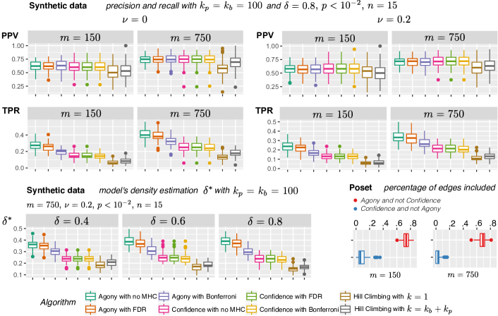
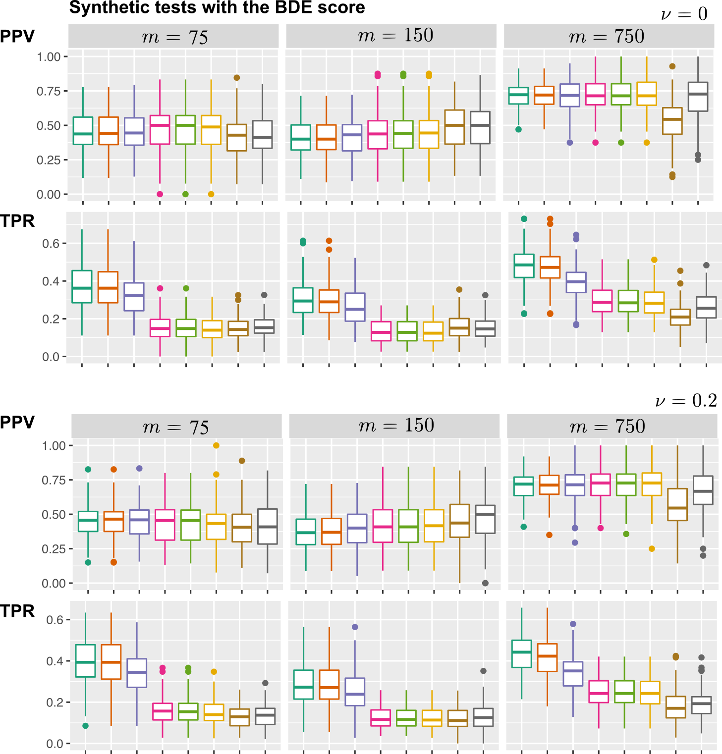
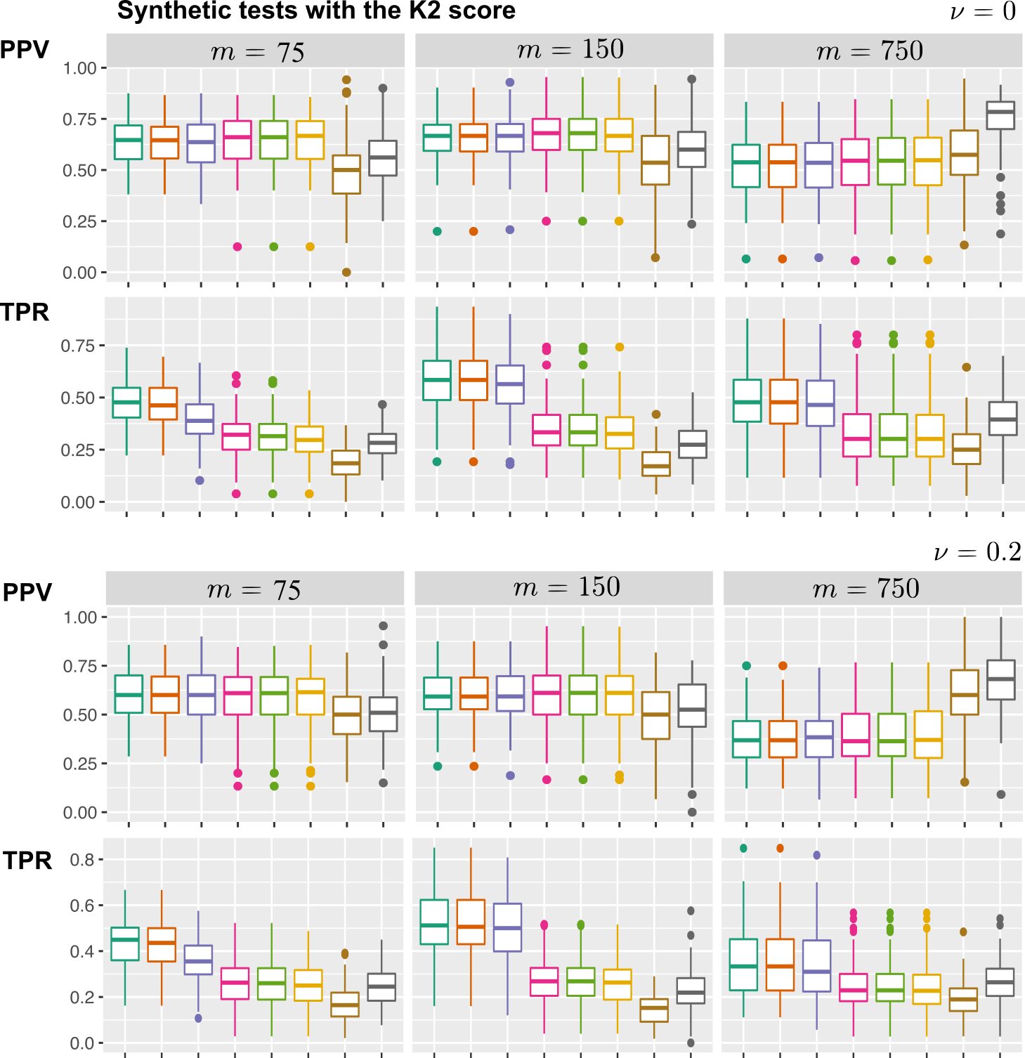
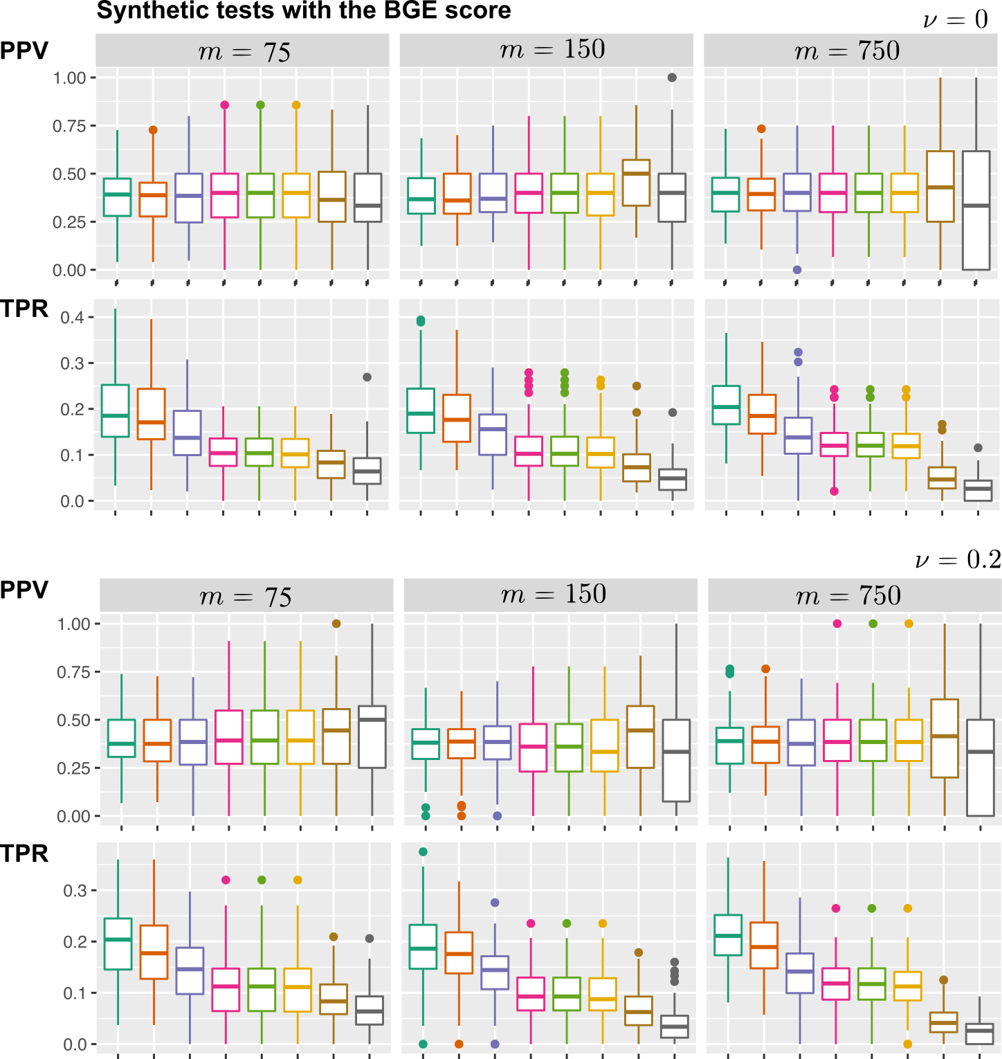
We carried out an extensive performance test that we recapitulate here and in the Supplementary Material. A summary of all the considered configurations is provided in Supplementary Table S1. The aim of the test is to assess which configuration of poset and hypotheses testing performs best for Algorithm 1, and compare its performance against Hill Climbing. We generated random networks (structures and parameteres) with different densities – i.e., number of edges with respect to number of variables – and various number of variables. From those BNs and a random (uniform) probability associated with each edge, we generated several datasets and perturbed them with different rates of false positives and negatives (noise). For each model inferred, we computed standard scores of precision (positive predictive value, ${\sf PPV}{}$) and recall (true positives rate TPR).

Results for discrete networks with the ${\sf f}={\sf BIC}$ are shown in Figure 4. For continuous networks (Gaussian) with also ${\sf f}={\sf AIC}$ in Supplementary Figure S8. Analogous tests for Bayesian scoring functions are in Supplementary Figures S9 (${\sf f}={\sf BDE}$), S10 (${\sf f}={\sf K2}$) and S11 (${\sf f}={\sf BGE}$). The comparison suggests that Algorithm 1 has a similar ability to retrieve true edges of Hill Climbing, PPV, but also a tendency to retrieve models with more edges, TPR. Thus, in all settings Algorithm 1 seems to improve remarkably over the baseline approach. The comparison suggests also that edge-selection by hypotheses testing seems less biased towards returning sparse models than a procedure based only on regularization. However, both approaches seem to converge towards fixed densities of the inferred model, with Algorithm 1 giving almost twice as many edges as Hill Climbing.

The effect of $k$ independent initial conditions for the Hill Climbing procedure does not seem to provide noteworthy improvements. Similarly, strategies for MHC do not seem to increase the performance in a particular way. For for agony, a stringent correction – FWER – seems too reduce TPR, while FDR does not seem to affect the scores. MHC does not seem to have any effect on the confidence poset. Interestingly, the comparison provides evidence that the agony poset is a superset of the confidence one, as the percentage of edges of the latter missing from the former approaches almost $0$. Other tests with these data suggest a minor improvement of performance if we use $1000$ bootstrap resamples, or different configurations of the parameters (data not shown). It is worth also to observe that, concerning the second bootstrap to create the null models, no major changes where detected for larger $k_{b}$; so in practice $k_{b}=100$ could be considered as a suitable value across multiple application domains.

5.2 The alarm network

Figure 5: Model selection for the alarm network with $m=10^{5}$ samples, and ${\sf f}={\sf BIC}$. We compare Hill Climbing with $k=0$ and $k=200$ ($\mathbf{D}\to_{{\sf f},\mathcal{M}}^{k}{\sf M}$) against Algorithm 1 with $k_{p}=k_{b}=100$. The left model of each pair is alarm, the right is ${\sf M}$. Edges are classified by color, depending which kind of false positive or negative they represent, and precision and recall scores are annotated. Algorithm 1 (confidence, FWER) achieves the best scores with Hill Climbing with $k=0$; for $k=200$ the Hill Climbing solution shows overfit. The models inferred by Algorithm 1 are strictly contained, and the confidence poset has higher scores than the agony poset.

Figure 6: For different sample size $m$ we generated $100$ datasets to generalize the comparison of Figure 5. The boxplots show the distributions of ${\sf PPV}{}$ and ${\sf TPR}{}$ for the alarm network with $m$ samples. The log-log plots show the gap of the p-value statistics for the two models computed by Algorithm 1 and shown in Figure 5.

We consider the standard alarm network [33] benchmark, as provided in the bnlearn package [26]. alarm has $n=37$ variables connected through 46 edges, for a total of 509 parameters.

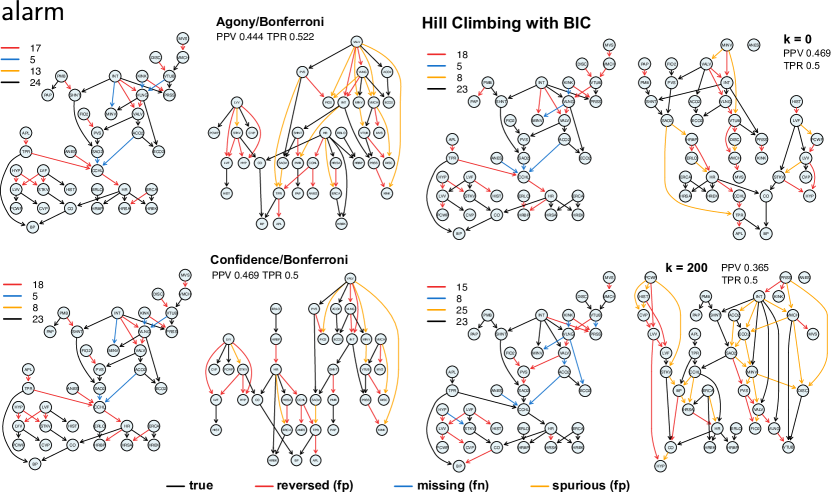
In Figure 5 we show the result of model selection for large samples size and ${\sf f}={\sf BIC}$. The comparison is performed against Hill Climbing with $k=0$ and $k=200$, whereas Algorithm 1 is executed with $k_{p}=k_{b}=100$. For large $m$, most setting seem to achieve the same performance; for lower $m$, highest PPV and TPR are achieved by Algorithm 1 (confidence, FWER). For this model, the use of multiple initial conditions for the Hill Climbing procedure reduces TPR; this is due to the number of spurious edges estimated, as the number of true positives is the same for $k=0$ and $k=200$. The models inferred by Algorithm 1 are strictly contained, and the confidence poset has higher scores than the agony one.

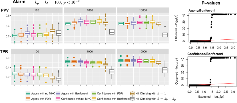
For this particular network we investigated also the effect of different sample size $m$, and the p-value for the statistical test on the performance of the algorithms. In Figure 6 we show boxplots obtained from $100$ datasets generated with different sample sizes. Results suggest minor changes in the performance with $m\geq 10^{3}$, and generalize the findings of Figure 5. Log-log plots show a consistent gap in the p-value statistics for the two models computed by Algorithm 1 shown in Figure 5. This is a phenomenon that we observed in all synthetic tests for sufficiently large $m$ (data not-shown), and that suggests the correctness of the statistical test in Algorithm 1.

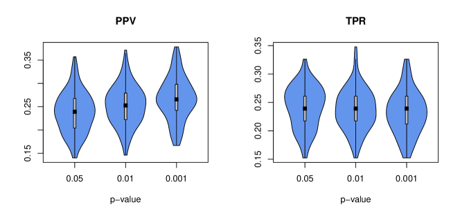
Analysis of the variation of the performance as a function of the p-values’ cutoff – for $p<0.05$, $p<10^{-2}$ and $p<10^{-3}$ with $m=100$ – shows small increase in PPV for lower p-values, but not meaningful changes in TPR scores (Supplementary Figure S12).

As a final remark, we note that with this dataset standard Hill Climbing without multiple restarts seems to achieve a better performance, compared to a search where multiple restarts are performed (see Figure 6). This behaviour might suggest the presence of a non-trivial relation underlying the ruggedness of the fitness landscape of the optimisation problem, and the role of restarts computed from correlated solutions. This kind of relation might require the development of more advanced resampling strategies, which could be approached leveraging on a bootstrap-based framework.

5.3 Modeling cancer evolution from genomic data

Figure 7: We estimated a model of progression of colorectal cancer (CRC) from a set of MSS tumors studied in [34]. Before inference, a set of boolean formulae is computed and added to the input data as new variables. These represent non-linear combinations of mutations and copy numbers alterations (CNAs) in the original genes, as computed in [34]. In top, we show the graphical notation of a formula that involves the genes activating the PI3K pathway; the intuition of a formula is to capture a functional module that is disrupted by mutations/ CNAs differently across all patients. The model is then obtained with $k_{p}=k_{b}=100$ and the same $\Pi_{\sf Suppes}$ estimated in [34] via Wilcoxon test ($p<0.05)$, after the marginal and conditional distributions are assessed with $k_{p}$ bootstrap resamples. In the test construction ($p<0.01$), we also use $100$ correlated restarts of the Hill Climbing to get better estimates for $\Gamma$. The linear progression model is due to Fearon and Vogelstein [35].

Cancers progress by accumulating genetic mutations that allow cancer cells to grow and proliferate out of control [36]. Mutations occur by chance, i.e., as a random process, and are inherited through divisions of cancer cells. The subset of mutations that trigger cancer growth by allowing a clone to expand, are called drivers [37]. Drivers, together with epigenetic alterations, orchestrate cancer initiation and development with accumulation and activation patterns differing between individuals [38]. This huge genotypic diversity – termed tumor heterogeneity – is thought to lead to the emergence of drug-resistance mechanisms and failure of treatments [39].

Major efforts are ongoing to decipher the causes and consequences of tumor heterogenity, and its relation to tumor progression (see, e.g., [40], and references therein). Here, we consider the problem of inferring a probabilistic model of cancer progression that recapitulates the temporal ordering, i.e., qualitative clocks, of the mutations that accumulate during cancer evolution [41]. We do this by scanning snapshots of cancer genomes collected via biopsy samples of several primary tumors; all the patients are untreated and diagnosed with the same cancer type (e.g., colorectal).

In this model-selection problem variables are $n$ somatic mutations detected by DNA sequencing – e.g., single-nucleotide mutations or chromosomal re-arrangements – annotated across $m$ independent samples. Thus, a sample is an $n$-dimensional binary vector: $\mathbb{B}=\{0,1\}$, and $\mathbf{x}_{i}=0$ if the $i$-th lesion is not detected in the patient’s cancer genome. We aim at inferring a model that accounts for the accumulation of the input variables during tumor evolution in different patients.

BNs do not encode explicitly this “cumulative” feature; however, they were recently combined with Suppes’ theory of probabilistic causation [42], which allows to describe cumulative phenomena. Suppes-Bayes Causal Networks (SBCNs, [43]) are BNs whose edges satisfy Suppes’ axioms for probabilistic causation, which mirror an expected “trend of selection” among the lesions, which is at the base of a Darwinian interpretation of cancer evolution [36]. Suppes’ conditions take the form of inequalities over pairs of variables that are evaluated before model-selection via a non-parametric bootstrap procedure. The model-selection’s landscape is then pruned of the edges that do not satisfy such conditions; thus, we can frame this as a poset

$$\Pi_{\sf Suppes}=\{\mathbf{x}_{i}\to\mathbf{x}_{j}\mid p(\mathbf{x}_{i})>p(\mathbf{x}_{j})\wedge p(\mathbf{x}_{j}\mid\mathbf{x}_{i})>p(\mathbf{x}_{j}\mid\neg\mathbf{x}_{i})\}$$ (11)

that we estimate from $\mathbf{D}$, along the lines of [44]. The parameters $\boldsymbol{\theta}$ of a SBCN will encode these conditions implicitly, rendering them suitable to model cumulative diseases such as cancer or other diseases [43].

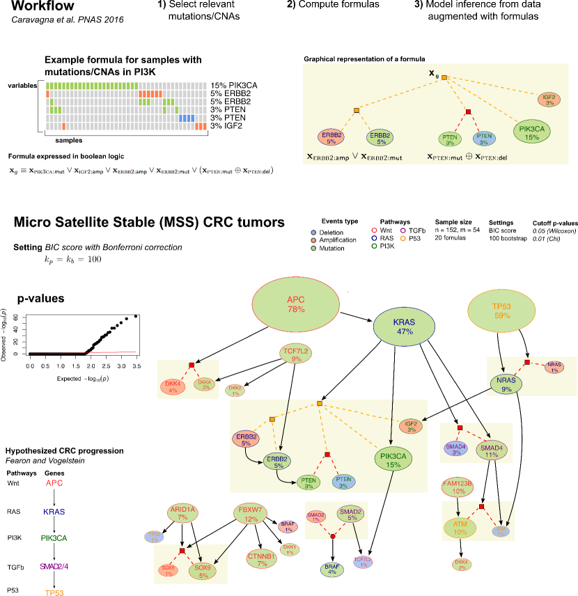
We will use data from [34], which collected and pre-processed high-quality genomics profiles from The Cancer Genome Atlas (TCGA). We consider a dataset of $m=152$ samples and $n=54$ variables, which refers to colorectal cancer patients with clinical Microsatellite Stable Status (MSS). The input data for MSS tumors consists in mutations (mut, mostly missense etc.) and copy numbers (amp, high-level amplifications; del, homozygous deletions) detected in $21$ genes of 5 pathways that likely drive colon cancer progression [45]. 20 out of $54$ variables are obtained as non-linear combinations of mutations and copy numbers in the original genes. For instance,

$$\mathbf{x}_{g}\equiv\mathbf{x}_{\text{\sc pik3ca}:{}\sf mut}\vee\mathbf{x}_{\text{\sc igf2}:{\sf amp}}\vee\mathbf{x}_{\text{\sc erbb2}:{\sf amp}}\vee\mathbf{x}_{\text{\sc erbb2}:{\sf mut}}\vee(\mathbf{x}_{\text{\sc pten}:{\sf mut}}\oplus\mathbf{x}_{\text{\sc pten}:{\sf del}})$$

is a variable $\mathbf{x}_{g}$ associated to the combination (in disjunctive $\vee$ and exclusive $\oplus$ form) of the events associated to the driver genes of the pi3k pathway pik3ca, igf2, erbb2 and pten. These new variables are called formulas (see [34] for a full list) and are included in $\mathbf{D}$ before assessment of Suppes’ conditions for two reasons. They capture the inter-patient heterogenity observed across the TCGA cohort (i.e., as biological “priors”). They limit the confounding effects of attempting inferences from hetergenous populations (i.e., as statistical “priors”).

We execute only the second part of our algorithm, i.e., the test, and compare the inferred model against the one obtained by Hill Climbing constrainted by $\Pi_{\sf Suppes}$ and with one initial condition (Figure 4 in [34]). In Figure 7 we show the model obtained with $k_{p}=k_{b}=100$ and the same $\Pi_{\sf Suppes}$ estimated in [34] via Wilcoxon test ($p<0.05)$ after the marginal and conditional distributions are assessed with $k_{p}$ bootstrap resamples. In the test construction ($p<0.01)$, we also use $100$ correlated restarts of the Hill Climbing to get better estimates for $\Gamma$.

We observe how our model is capable of capturing a lot of known features of MSS tumors as described in the seminal work of [35]. In fact, we find APC as the main gene starting the progression followed by KRAS. Afterward, we observe multiple branches, yet involving genes from the PI3K (i.e., PIK3CA) and TGFb (i.e., SMAD2 and SMAD4) pathways, which are suggested to be later events during tumorigenesis of MSS tumors. While TP53 is not inferred to be a late event in the progression, we still find the P53 pathway to be involved in advanced tumors with ATM being one of the final nodes in one branch of the model. We remark that this tumor type shows considerable heterogeneity across different patients [46], and evidences of TP53 as an early event in this cancer’s progression have been found [47].

6 Conclusions

In this paper we consider the identification of a factorization of a BN without hidden variables. This model-selection task is central to problems in statistics that require the learning of a joint distribution made compact by retaining only the relevant conditional dependencies in the data.

A common approach to it consists of a heuristic search over the space of factorizations, the result being the computation of the MLE of the structure and the parameters of the model, or of a marginalised likelihood over the structures. Surprisingly, the simple Hill-Climbing search strategy augmented with a regularized score function, provides satisfactory baseline performance [6].

Here, we derive an algorithm based on bootstrap and multiple hypothesis testing that, compared to baseline greedy optimization, achieves consistently better model estimates. This result can stimulate further studies on the theoretical relation between the $\log$-likelihood function of a BN and greedy optimization, and attempts also at unifying two streams of research in BN model-selection.

On one side, we draw inspiration from the seminal works by Friedman et al. which investigated whether we can assess “if the existence of an edge between two nodes is warranted”, or if we “can say something of the ordering of two variables” [12]. Precisely, Friedman et al. answered to these questions by showing that high-confidence estimates on certain structural features, when assessed by a non-parametric bootstrap strategy, can be “indicative of the existence of these features in the generative model”.

On the other side, we follow the suggestion by Teyssier and Koeller on the well-known fact that the best network consistent with a given node ordering can be found very efficiently [13]. Teyssier and Koeller consider BNs of bounded in-degree, and “propose a search not over the space of structures, but over the space of orderings, selecting for each ordering the best network consistent with it”. Their motivation is driven by algorithmic an argument: “[the orderings’] search space is much smaller, makes more global search steps, has a lower branching factor, and avoids costly acyclicity checks”.

Here, we connect the two observations in one framework. We first estimate orderings via non-parametric bootstrap, combined with greedy estimation of the model in each resample. Then, after rendering the model acyclic, we use it to select one final model that is consistent with the orderings. Our approach improves regardless of the information-theoretic or Bayesian scoring function adopted. To this extent, we use the orderings as an empirical Bayes prior over model structures, and compute the maximum a posteriori estimate of the model. The parameters are then the MLE estimates for the selected structure. Our result is based on a refinement of the original observation by Teyssier and Koller: when we know the ordering, besides improving complexity we enjoy a systematic reduction in the “statistical” complexity in the problem of identifying true dependencies. We postulate this after observing that with the best possible ordering – i.e., a transitive closure of the generative model – the fitness landscape becomes unimodal.

Acknowledgement.

Both the authors wish to thank Guido Sanguinetti and Dirk Husmeier for useful discussions on a preliminary version of this manuscript.

Appendix A Supplementary Tables

The following tables are provided.

$\#$Simulations	Variables	$\#$Node	Sample Size	Density	Noise Level
$100$	Binary	$15$	$\{75,150,750\}$	$\{0.4,0.6,0.8\}$	$\{0.0,0.2\}$
$100$	Binary	$10$	$\{50,100\}$	$\{0.4,0.6\}$	$\{0.0,0.2\}$
$100$	Continuous	$10$	$\{50,100\}$	$\{0.4,0.6\}$	$\{0.0,0.2\}$

Table S1: Performed synthetic tests. In this table we summarize the performed simulations. Namely, we considered $3$ settings; the first two for Bayesian Networks respectively of $10$ and $15$ binary variables, different sample sizes and network densities. In the third experiment, we considered a similar configuration to experiment $2$ but we now simulate continuous variables. For all datasets, we considered both the noise free case and the one with $20\%$ noise. We performed 100 independent simulations for each configuration. This led us to a total of $3400$ synthetic datasets.

Appendix B Supplementary Figures

The following figures are provided.

• Figure S8: synthetic tests with different settings from Figure 4.

• Figure S9, S10 and S11: synthetic tests analogous to the ones from Figure 4 for Bayesian scoring functions.

• Figure S12: the effects of different p-values on the model-selection for the alarm network.

Figure S8: Synthetic tests with different settings from Figure 4: top, f=AIC, mid, $\delta=0.4$, and bottom, continuous variables. In left, for $n$ the number of nodes in the model, we generate $10*n$ samples, in right $50*n$.

Figure S9: Synthetic tests with binary variables for the BDE Bayesian score. We observe that these simulations, as well as those for other Bayesian scores (Supplementary Figures S10 and S11) show similar trends to the ones discussed in the main text for information-theoretic scoring functions.

Figure S10: Synthetic tests with binary variables for the K2 Bayesian score.

Figure S11: Synthetic tests with Gaussian variables for the BGE Bayesian score.

Figure S12: Violin plots for different p-values $p$ on the model-selection for the alarm network with the agony poset and Bonferroni correction. $100$ random datasets are generated with $m=100$ samples. The same settings of Figure 6 are used.

References

- [1] Judea Pearl. Probabilistic reasoning in intelligent systems: networks of plausible inference. Morgan Kaufmann, 1988.
- [2] Daphne Koller and Nir Friedman. Probabilistic graphical models: principles and techniques. MIT press, 2009.
- [3] David Maxwell Chickering, David Heckerman, and Christopher Meek. Large-sample learning of Bayesian Networks is NP-hard. The Journal of Machine Learning Research, 5:1287–1330, 2004.
- [4] Robert W Robinson. Counting unlabeled acyclic digraphs. In Combinatorial mathematics V, pages 28–43. Springer, 1977.
- [5] Judea Pearl and Thomas S Verma. A theory of inferred causation. Studies in Logic and the Foundations of Mathematics, 134:789–811, 1995.
- [6] José A Gámez, Juan L Mateo, and José M Puerta. Learning Bayesian networks by hill climbing: efficient methods based on progressive restriction of the neighborhood. Data Mining and Knowledge Discovery, 22(1):106–148, 2011.
- [7] Gideon Schwarz. Estimating the dimension of a model. The annals of statistics, 6(2):461–464, 1978.
- [8] Hirotogu Akaike. Information theory and an extension of the maximum likelihood principle. In Selected Papers of Hirotugu Akaike, pages 199–213. Springer, 1998.
- [9] Gregory F Cooper and Edward Herskovits. A Bayesian method for the induction of probabilistic networks from data. Machine learning, 9(4):309–347, 1992.
- [10] Dan Geiger and David Heckerman. Learning gaussian networks. In Proceedings of the Tenth international conference on Uncertainty in artificial intelligence, pages 235–243. Morgan Kaufmann Publishers Inc., 1994.
- [11] Bradley Efron and Robert J Tibshirani. An Introduction to the Bootstrap. CRC press, 1994.
- [12] Nir Friedman, Moises Goldszmidt, and Abraham Wyner. Data analysis with Bayesian Networks: a bootstrap approach. In Proceedings of the Fifteenth conference on Uncertainty in artificial intelligence, pages 196–205. Morgan Kaufmann Publishers Inc., 1999.
- [13] Marc Teyssier and Daphne Koller. Ordering-based search: A simple and effective algorithm for learning Bayesian Networks. arXiv preprint arXiv:1207.1429, 2012.
- [14] David Maxwell Chickering. Learning equivalence classes of Bayesian Network structures. Journal of machine learning research, 2(Feb):445–498, 2002.
- [15] Nir Friedman and Daphne Koller. Being Bayesian about network structure. a Bayesian approach to structure discovery in Bayesian Networks. Machine learning, 50(1-2):95–125, 2003.
- [16] Marco Grzegorczyk and Dirk Husmeier. Improving the structure mcmc sampler for bayesian networks by introducing a new edge reversal move. Machine Learning, 71(2):265–305, 2008.
- [17] Robert JB Goudie and Sach Mukherjee. A gibbs sampler for learning dags. The Journal of Machine Learning Research, 17(1):1032–1070, 2016.
- [18] Jack Kuipers and Giusi Moffa. Partition mcmc for inference on acyclic digraphs. Journal of the American Statistical Association, 112(517):282–299, 2017.
- [19] Mikko Koivisto and Kismat Sood. Exact bayesian structure discovery in bayesian networks. Journal of Machine Learning Research, 5(May):549–573, 2004.
- [20] Daniel Eaton and Kevin Murphy. Exact bayesian structure learning from uncertain interventions. In Artificial intelligence and statistics, pages 107–114, 2007.
- [21] James Cussens. Bayesian network learning with cutting planes. arXiv preprint arXiv:1202.3713, 2012.
- [22] James Cussens, Matti Järvisalo, Janne H Korhonen, and Mark Bartlett. Bayesian network structure learning with integer programming: Polytopes, facets and complexity. Journal of Artificial Intelligence Research, 58:185–229, 2017.
- [23] Marco Scutari, Catharina Elisabeth Graafland, and José Manuel Gutiérrez. Who learns better bayesian network structures: Accuracy and speed of structure learning algorithms. International Journal of Approximate Reasoning, 115:235–253, 2019.
- [24] Mauro Scanagatta, Antonio Salmerón, and Fabio Stella. A survey on bayesian network structure learning from data. Progress in Artificial Intelligence, pages 1–15, 2019.
- [25] Dominique MA Haughton et al. On the choice of a model to fit data from an exponential family. The Annals of Statistics, 16(1):342–355, 1988.
- [26] Marco Scutari. Learning Bayesian Networks with the bnlearn R package. Journal of Statistical Software, 35(i03), 2010.
- [27] Richard M Karp. Reducibility among combinatorial problems. In Complexity of computer computations, pages 85–103. Springer, 1972.
- [28] Viggo Kann. On the approximability of NP-complete optimization problems. PhD thesis, Royal Institute of Technology Stockholm, 1992.
- [29] Charles AR Hoare. Quicksort. The Computer Journal, 5(1):10–16, 1962.
- [30] Thomas H Cormen. Introduction to algorithms. MIT press, 2009.
- [31] Mangesh Gupte, Pravin Shankar, Jing Li, Shanmugauelayut Muthukrishnan, and Liviu Iftode. Finding hierarchy in directed online social networks. In Proceedings of the 20th international conference on World wide web, pages 557–566. ACM, 2011.
- [32] Nikolaj Tatti. Hierarchies in directed networks. In Data Mining (ICDM), 2015 IEEE International Conference on, pages 991–996. IEEE, 2015.
- [33] Ingo A Beinlich, Henri J Suermondt, R Martin Chavez, and Gregory F Cooper. The ALARM monitoring system: A case study with two probabilistic inference techniques for belief networks. Springer, 1989.
- [34] Giulio Caravagna, Alex Graudenzi, Daniele Ramazzotti, Rebeca Sanz-Pamplona, Luca De Sano, Giancarlo Mauri, Victor Moreno, Marco Antoniotti, and Bud Mishra. Algorithmic methods to infer the evolutionary trajectories in cancer progression. Proceedings of the National Academy of Sciences, 113(28):E4025–E4034, 2016.
- [35] Eric R Fearon, Bert Vogelstein, et al. A genetic model for colorectal tumorigenesis. Cell, 61(5):759–767, 1990.
- [36] Peter C Nowell. The clonal evolution of tumor cell populations. Science, 194(4260):23–28, 1976.
- [37] Bert Vogelstein and Kenneth W Kinzler. Cancer genes and the pathways they control. Nature Medicine, 10(8):789–799, 2004.
- [38] Franziska Michor, Yoh Iwasa, and Martin A Nowak. Dynamics of cancer progression. Nature Reviews Cancer, 4(3):197–205, 2004.
- [39] Charles Swanton. Intratumor heterogeneity: evolution through space and time. Cancer research, 72(19):4875–4882, 2012.
- [40] Andriy Marusyk and Kornelia Polyak. Tumor heterogeneity: causes and consequences. Biochimica et Biophysica Acta (BBA)-Reviews on Cancer, 1805(1):105–117, 2010.
- [41] Niko Beerenwinkel, Roland F Schwarz, Moritz Gerstung, and Florian Markowetz. Cancer evolution: mathematical models and computational inference. Systematic biology, 64(1):e1–e25, 2015.
- [42] Patrick Suppes. A probabilistic theory of causation, 1970.
- [43] Daniele Ramazzotti, Alex Graudenzi, Giulio Caravagna, and Marco Antoniotti. Modeling cumulative biological phenomena with suppes-bayes causal networks, 2017.
- [44] Daniele Ramazzotti, Giulio Caravagna, Loes Olde Loohuis, Alex Graudenzi, Ilya Korsunsky, Giancarlo Mauri, Marco Antoniotti, and Bud Mishra. Capri: efficient inference of cancer progression models from cross-sectional data. Bioinformatics, 31(18):3016–3026, 2015.
- [45] The Cancer Genome Atlas Network et al. Comprehensive molecular characterization of human colon and rectal cancer. Nature, 487(7407):330–337, 2012.
- [46] Justin Guinney, Rodrigo Dienstmann, Xin Wang, Aurélien de Reyniès, Andreas Schlicker, Charlotte Soneson, Laetitia Marisa, Paul Roepman, Gift Nyamundanda, Paolo Angelino, et al. The consensus molecular subtypes of colorectal cancer. Nature medicine, in print, 2015.
- [47] Noa Rivlin, Ran Brosh, Moshe Oren, and Varda Rotter. Mutations in the p53 tumor suppressor gene important milestones at the various steps of tumorigenesis. Genes & cancer, 2(4):466–474, 2011.