Sparse Wavelet Estimation in Quantile Regression with Multiple Functional Predictors

Abstract

In this manuscript, we study quantile regression in partial functional linear model where response is scalar and predictors include both scalars and multiple functions. Wavelet basis are adopted to better approximate functional slopes while effectively detect local features. The sparse group lasso penalty is imposed to select important functional predictors while capture shared information among them. The estimation problem can be reformulated into a standard second-order cone program and then solved by an interior point method. We also give a novel algorithm by using alternating direction method of multipliers (ADMM) which was recently employed by many researchers in solving penalized quantile regression problems. The asymptotic properties such as the convergence rate and prediction error bound have been established. Simulations and a real data from ADHD-200 fMRI data are investigated to show the superiority of our proposed method.

Keywords: Functional data analysis; Sparse group lasso; ADMM; Convergence rate; Prediction error bound; ADHD

1 Introduction

Functional data analysis (FDA) is about the analysis of information on curves, images, functions, or more general objects. It has become a major branch of nonparametric statistics and is a fast evolving area as more data has arisen where the primary object of observation can be viewed as a function (Ramsay, 2006; Wang et al., 2015; Morris, 2015). A standard functional linear model with scalar response and functional covariate is

$$y=\alpha+\int_{0}^{1}x(t)\beta(t)dt+\varepsilon,$$ (1)

where the coefficient $\beta(t)$ is a function, and $\varepsilon$ is a random error. To estimate the functional coefficient $\beta(t)$, we can use functional basis to approximate it. There are three major choices of functional basis: general basis such as B-spline basis and wavelet basis (Cardot et al., 2003; Zhao et al., 2012), functional principal component basis (Cardot et al., 1999; Cai and Hall, 2006; Müller and Yao, 2008; Kong et al., 2016), and partial least square basis (Delaigle and Hall, 2012). Recently in imaging analysis, Zhao et al. (2012), Wang et al. (2014) and Zhao et al. (2015) successfully adopted wavelet basis with regularizations to estimate the functional slope where the functional covariates are image features located in 1D, 2D and 3D domains respectively.

The functional linear model (1) can be extended to a partial functional linear model with multiple functional covariates

$$y=\alpha+\int_{0}^{1}\bm{x}^{T}(t)\bm{\beta}(t)dt+\bm{u}^{T}\bm{\gamma}+\varepsilon,$$ (2)

where covariates $\bm{u}$ are scalars and $\bm{\gamma}$ are the coefficients. The functional coefficients $\bm{\beta}(t)$ can be estimated by using regularization techniques. In particular, penalized principal component basis has been an especially popular choice (Gertheiss et al., 2013; Lian, 2013). Recently, Kong et al. (2016) successfully applied such technique to model (2) in the setting of ultrahigh-dimensional scalar predictors.

In recent years, quantile regression, which was introduced by the seminal work of Koenker and Bassett (1978), has been well developed and recognized in functional linear regression, with many mainly focusing on the functional linear quantile regression model:

$$Q_{\tau}(y|x(t))=\alpha_{\tau}+\int_{0}^{1}x(t)\beta_{\tau}(t)dt,$$ (3)

where $Q_{\tau}(y|x(t))$ is the $\tau$-th conditional quantile of response $y$ given a functional covariate $x(t)$ for a fixed quantile level $\tau\in(0,1)$. As an alternative to least squares regression, the quantile regression method is more efficient and robust when the responses are non-normal, errors are heavy tailed or outliers are present. It is also capable of dealing with the heteroscedasticity issues and providing a more complete picture of the response (Koenker, 2005). To estimate the functional coefficient $\beta_{\tau}(t)$, functional basis can as well be used to approximate it; for instance, general basis like B-spline basis (Cardot et al., 2005; Sun, 2005), functional principle component basis (Kato, 2012; Lu et al., 2014; Tang and Cheng, 2014) and partial quantile basis (Yu et al., 2016).

In this article, we extend model (3) to a partial functional linear quantile regression model with multiple functional covariates

$$Q_{\tau}(y|~{}\bm{u},\bm{x}(t))=\alpha_{\tau}+\int_{0}^{1}\bm{x}^{T}(t)\bm{\beta}_{\tau}(t)dt+\bm{u}^{T}\bm{\gamma}_{\tau},$$ (4)

where $Q_{\tau}(y|~{}\bm{u},\bm{x}(t))$ is the $\tau$-th conditional quantile of $y$ given scalar covariates $\bm{u}$ and multiple functions $\bm{x}(t)$. To our best knowledge, only a few works have studied this model; for example, Yu et al. (2016) used partial quantile basis while Yao et al. (2017) used penalized principal component basis. Inspired by the success of wavelet basis with regularization in functional linear model (Zhao et al., 2012; Wang et al., 2014; Zhao et al., 2015), we use it to approximate the functional coefficients $\bm{\beta}_{\tau}(t)$ in model (4). Wavelet basis can provide a good representation of functional coefficients by using only a small number of basis and are particularly useful for capturing localized functional features. Moreover, the wavelet transform is computationally efficient and hence suitable for dealing with multiple functional predictors.

The penalization we impose is sparse group lasso (Zhao et al., 2014, Simon et al., 2013), which is motivated by the attention deficit hyperactivity disorder (ADHD) study from the ADHD-200 Sample Initiative Project. Our goal is to predict ADHD index at various quantile levels by using both demographic information and functional magnetic resonance imaging (fMRI) data, where the fMRI data consists of $116$ functional features, each of which represents a single region of interests (ROI) of human brain. The sparse group lasso technique, by imposing a convex combination of lasso and group lasso penalties, can select important ROIs while capture shared information among them. More specifically, the group lasso penalty makes a sparse selection out of $116$ functional features of ROIs, while the lasso penalty induces a sparse representation of each feature. Common wavelet basis is used to represent different features so that the shared information among them can be captured.

There are five major contributions of this paper. First, our conditional quantile framework provides a more suitable modelling of reality especially when the response is heavy tailed (Yao et al., 2017). It is also a compelling choice of dealing with heteroscedasticity issues and can provide a more complete picture of the response (Koenker, 2005). Second, the wavelet basis we adopt provides a good approximation of functional coefficients while effectively detects the local features. The wavelet transform we use is computationally efficient and hence can be easily extended to deal with multiple functional predictors. Third, the proposed sparse group lasso method selects important functional predictors and retains shared information among them as well. It is extremely useful in ADHD-200 fMRI study so that both individual and common information can be captured among the different ROIs. Fourth, the estimation problem is in fact a penalized quantile regression problem, which can be reformulated into a second-order cone program and then easily solved by an interior point method implemented by a powerful R package: Rmosek. We also propose a novel algorithm to solve it by using alternating direction method of multipliers (ADMM). Fifth, we successfully derive the asymptotic properties including the convergence rate and prediction error bound which theoretically warrants good performance of our estimates.

The rest of paper is organized as follows. In Section 2, we review some necessary background on wavelets and provide the penalized quantile objective function with sparse group lasso penalty. The asymptotic properties such as the convergence rate and predictor error bound are established in Section 3. In Section 4, the quantile penalization problem is reformulated into a second-order cone program (SOCP) and solved by an interior point method by using a powerful R package: Rmosek. We also propose a novel algorithm using alternating direction method of multipliers (ADMM). Finite sample simulations and a real data from ADHD-200 fMRI data are investigated in Section 5 to illustrate the superiority of our proposed method.

2 Wavelet-based Sparse Group Lasso

In this section, we first review some necessary background on wavelets. We then provide the penalized quantile objective function with sparse group lasso penalty where the functional coefficients are approximated by wavelet basis. This leads to the sparsities of both the selection and representation of functional features. More specifically, the group lasso selects a sparse set from available functional features, while the lasso induces a sparse representation of the selected functional features.

2.1 Some Background on Wavelets

Wavelets are basis function that can provide a good approximation of functional coefficients while effectively capture the local features (Zhao et al., 2012). Moreover, the wavelet transform is computationally efficient and hence can be easily extended to deal with multiple functional predictors (Daubechies, 1990). For a given $\tau\in(0,1)$, let $\beta_{l\tau}(t)$ be one component of $\bm{\beta}_{\tau}(t)$ in (4), where $\bm{\beta}_{\tau}(t)=(\beta_{1\tau}(t),\ldots,\beta_{m\tau}(t))^{T}$. Suppose that $\beta_{l\tau}(t)$ is in $L^{2}[0,1]$. We can approximate it using wavelet basis. For any wavelet basis in $L^{2}[0,1]$, they can be derived by dilating and translating two orthonormal basic functions: a scaling function and a wavelet function, namely $\phi(t)$ and $\psi(t)$ respectively:

$$\varphi_{jk}(t)=\sqrt{2^{j}}\varphi(2^{j}t-k),\ \ \ \ \psi_{jk}(t)=\sqrt{2^{j}}\psi(2^{j}t-k),$$

where $j$ and $k$ are integers, $\int_{0}^{1}\varphi(t)=1$ and $\int_{0}^{1}\psi(t)=0$. In particular, given a primary resolution level $j_{0}$, the wavelet basis are

$$\{\varphi_{j_{0},k}\}_{0\leq k\leq 2^{j_{0}}-1}\quad\rm{and}\quad\{\psi_{j,k}\}_{j_{0}\leq j,\ 0\leq k\leq 2^{j}-1}.$$ (5)

Therefore, $\beta_{l\tau}(t)$ can be approximated by

$$\beta_{l\tau}(t)=\sum_{k=0}^{2^{j_{0}}-1}a_{j_{0}k}^{l}\varphi_{j_{0}k}(t)+\sum_{j=j_{0}}^{\infty}\sum_{k=0}^{2^{j}-1}d_{jk}^{l}\psi_{jk}(t),\ \ \ \ \ \rm{for}~{}~{}l=1,\dots,m,$$ (6)

where $a_{j_{0}k}^{l}=\int_{0}^{1}\beta_{l\tau}(t)\varphi_{j_{0},k}(t)dt$ is the approximation coefficients at the coarsest resolution $j_{0}$, and $d_{jk}^{l}=\int_{0}^{1}\beta_{l\tau}(t)\psi_{jk}(t)dt$ is the detail coefficients characterizing the fine structures.

In practice, the functional covariates $\bm{x}(t)=(x_{1}(t),\ldots,x_{m}(t))^{T}$ are discretely observed, for instance without loss of generality, at $N=2^{J}$ equally spaced points of $[0,1]$ with $0=t_{1}<t_{2}<\cdots<t_{N}=1$. Let $\bm{X}=(\bm{x}_{1},\ldots,\bm{x}_{m})$ and $\bm{\beta}_{\tau}=(\bm{\beta}_{1\tau},\ldots,\bm{\beta}_{m\tau})$, where $\bm{x}_{l}=(x_{1}(t_{1}),\ldots,x_{m}(t_{N}))^{T}$, $\bm{\beta}_{l\tau}=(\beta_{l\tau}(t_{1}),\ldots,\beta_{l\tau}(t_{N}))^{T}$ and $l=1,\ldots,m$. We represent $\bm{X}$ and $\bm{\beta}_{\tau}$ by the wavelet coefficients through discrete wavelet transform (DWT). In particular, let $\bm{W}$ be an $N\times N$ matrix associated with orthonormal wavelet basis derived from DWT. Suppose $\bm{C}$ and $\bm{B}$ are the corresponding wavelet coefficients of $\bm{X}$ and $\bm{\beta}_{\tau}$. Then we have $\bm{X}=\bm{W}^{T}\bm{C}$, $\bm{\beta}_{\tau}=\bm{W}^{T}\bm{B}_{\tau}$, and the integration in model (4):

$$\int_{0}^{1}\bm{x}^{T}(t)\bm{\beta}_{\tau}(t)dt\approx\rm{vec}(\bm{X})^{T}\rm{vec}(\bm{\beta}_{\tau})/N=\rm{vec}(\bm{W}^{T}\bm{C})^{T}\rm{vec}(\bm{W}^{T}\bm{B})/N=\rm{vec}(\bm{C})^{T}\rm{vec}(\bm{B})/N.$$

The last equality holds due to the orthonormality of $\mathbf{W}$. From now on, we denote $\bm{v}=\rm{vec}(\bm{C})^{T}/N$ and $\bm{\theta}_{\tau}=\rm{vec}(\bm{B})$ where $\bm{C}=(\bm{c}_{1},\ldots,\bm{c}_{m})$ and $\bm{B}=(\bm{b}_{1\tau},\ldots,\bm{b}_{m\tau})$.

2.2 Model Estimation

Using wavelet basis by DWT, model (4) becomes

$$Q_{\tau}(y|\bm{u},\bm{x}(t))\approx\alpha_{\tau}+\bm{v}^{T}\bm{\theta}_{\tau}+\bm{u}^{T}\bm{\gamma}_{\tau}.$$ (7)

Given $n$ identical copies of data triplets $(\bm{X}_{i},\bm{u}_{i},y_{i})$, where $\bm{X}_{i}$ and $\bm{u}_{i}$ are the observed functional and scalar covariates respectively, and $y_{i}$ is the corresponding response, the parameters in (7) can be estimated by minimizing a regular quantile loss function. However, to find the important functional covariates in predicting responses while preserve a desired sparse representation of the coefficients, an appropriate penalty has to be imposed. In this paper, we propose to use the sparse group lasso penalty

$$P_{\lambda_{1},\lambda_{2}}(\bm{\theta})=\lambda_{1}\sum_{l=1}^{m}||\bm{b}_{l}||_{1}+\lambda_{2}\sum_{l=1}^{m}||\bm{b}_{l}||_{2},$$ (8)

where $||\cdot||_{1}$ and $||\cdot||_{2}$ represent the $L_{1}$ and $L_{2}$ norms respectively, and $\lambda_{1}$ and $\lambda_{2}$ are two nonnegative tuning parameters. The sparse group lasso penalty includes two components, namely a lasso and a group lasso penalties, where the lasso penalty $||\cdot||_{1}$ induces sparsity in each functional coefficient and the group lasso penalty $||\cdot||_{2}$ selects functional coefficients. Common information among functional covariates can be retained by using the same wavelet basis to approximate the functional coefficients. Moreover, the sparse group lasso warrants the selection of important functional coefficients while captures distinct traits carried by individual functional covariates. Specifically, the parameters $\alpha_{\tau}$, $\bm{\gamma}_{\tau}$, and $\bm{\theta}_{\tau}$ can be estimated by

$$(\hat{\alpha}_{\tau},\hat{\bm{\gamma}}_{\tau},\hat{\bm{\theta}}_{\tau})=\underset{\alpha,\bm{\gamma},\bm{\theta}}{\arg\min}\sum_{i=1}^{n}\rho_{\tau}\big{(}y_{i}-\alpha-\bm{u}_{i}^{T}\bm{\gamma}-\bm{v}_{i}^{T}\bm{\theta}\big{)}+P_{\lambda_{1},\lambda_{2}}(\bm{\theta}),$$ (9)

where $\rho_{\tau}(x)=x(\tau-\mathbf{1}(x<0))$ is the quantile check function (Koenker, 2005).

To combine information from different quantiles, Zou and Yuan (2008) proposed composite quantile regression, which simultaneously considers multiple regression quantiles at different levels. With homoscedasticity assumption, where all conditional regression quantiles have the same slope, the composite quantile estimate is more efficient than the one from a single level and has in recent years begun to gain its popularity in many fields (Kai et al., 2010; Fan and Lv, 2010; Bradic et al., 2011, Kai et al., 2011; Yu et al., 2016). In this paper, we propose to use composite quantile regression with sparse group lasso penalty in our functional data analysis framework. Let $0<\tau_{1}<\dots<\tau_{k}<1$ denote the selected quantile levels and then the parameters ${\bm{\alpha}},{\bm{\gamma}}$ and ${\bm{\theta}}$ can be estimated by

$$(\hat{\bm{\alpha}},\hat{\bm{\gamma}},\hat{\bm{\theta}})=\underset{{\bm{\alpha}},{\bm{\gamma}},{\bm{\theta}}}{\arg\min}\sum_{k=1}^{K}\sum_{i=1}^{n}{\rho}_{\tau_{k}}(y_{i}-\alpha_{k}-\bm{u}_{i}^{T}\bm{\gamma}-\bm{v}_{i}^{T}\bm{\theta})+P_{\lambda_{1},\lambda_{2}}(\bm{\theta}),$$ (10)

where $\bm{\alpha}=(\alpha_{1}.\dots,\alpha_{{K}})$ is a vector of intercepts. Typically, we can choose $K=9$ and use equally spaced quantiles (Kai et al., 2010; Zou and Yuan, 2008). Note that quantile estimate (9) at a single level is just a special case of composite quantile estimate (10) with $K=1$. In the following, we will focus on the composite quantile regression case of (10).

3 Asymptotics

In this section, we investigate the asymptotic properties of our proposed estimates when both the sample size $n$ and the number of discrete points $N_{n}$ tend to infinity. Let $\lambda_{1,n}$ and $\lambda_{2,n}$ denote the tuning parameters when the sample size is $n$. To derive the asymptotic properties, we impose the following conditions:

1. A1.   The model errors $\varepsilon_{1},\ldots,\varepsilon_{n}$ are independently following a distribution $F$, with density $f$ to be bounded away from zero and infinity, and its derivative $f^{\prime}$ to be continuous and uniformly bounded.

2. A2.    There exist two constants $c_{1}$ and $c_{2}$ such that

   $$0<c_{1}<\varrho_{\min}(\frac{1}{n}\bm{A}_{n}^{T}\bm{A}_{n})\leq\varrho_{\max}(\frac{1}{n}\bm{A}_{n}^{T}\bm{A}_{n})<c_{2}<\infty,$$

   where $\bm{A}_{n}=(\bm{a}_{1},\ldots,\bm{a}_{n})^{T}$ is the design matrix with $\bm{a}_{i}=(1,\bm{v}_{i}^{T},\bm{u}_{i}^{T})^{T}$, and $\varrho_{\min}(\cdot)$ and $\varrho_{\max}(\cdot)$ are the smallest and largest eigenvalues of $\frac{1}{n}\bm{A}_{n}^{T}\bm{A}_{n}$ respectively.

3. A3.    There exists a constant $M$ such that $||\bm{a}_{i}||_{2}<M$ for all $i$.

4. A4.    The functional slope $\beta_{l}(t)$s are $d$ times differentiable in the Sobolev sense, and the wavelet basis has $w$ vanishing moments, where $w>d.$

5. A5.   $\lambda_{1,n}=O(\sqrt{n})$ and  $\lambda_{2,n}=O(\sqrt{n})$.

6. A6.   $N_{n}/n\to 0$.

These regularity conditions might not be the weakest ones but are commonly assumed among literatures of quantile regression and functional linear model. Condition (A1) is standard for quantile regression (Koenker, 2005; Zhao et al., 2014), which regulates the behavior of the conditional density of the response in a neighborhood of the conditional quantile and is crucial to the asymptotic properties of quantile estimators (Koenker and Bassett, 1978). Condition (A2) is a classical condition in functional linear regression literature (Delaigle and Hall, 2012). It ensures the eigenvalues of the covariance matrix go to neither zero nor infinity too quickly. Similar conditions as (A3) - (A6) can be found in Zhao et al. (2012) and Zhao et al. (2015), among others. Condition (A4) guarantees that the space spanned by the wavelet basis can well approximate the functional slopes with small approximation errors. Condition (A6) implies that to allow for estimation of $\beta$ with appropriate asymptotic properties, $n$ should grow faster than $N_{n}$. Note the wavelet basis has $w$ vanishing moments if and only if its scaling function $\varphi$ can generate polynomials of degree at most $w$.

Theorem 3.1.

Let $\hat{\beta}_{l,n}$ be the estimator resulting from (10) and $\beta_{l}$ is the true coefficient function. If Conditions (A1)-(A6) hold, then

$$||\hat{\beta}_{l,n}-\beta_{l}||_{2}^{2}=O_{p}\left({\frac{N_{n}}{n}}\right)+o_{p}\left(\frac{1}{N_{n}^{2d}}\right).$$

A detailed proof of this theorem is provided in the Appendix. The accuracy of $\hat{\beta}$ relies on both $n$ and $N_{n}$. The approximation error rate of $\hat{\beta}$ towards $\beta$ are controlled by two terms. The first term is of the same order of $N_{n}/n$ which is a typical result of estimating, while the second term is of the lower order of $1/N_{n}^{2d}$ which is mainly due to approximation by wavelets. In particular, the approximation error rate is dominated by the second term if $N_{n}^{2d+1}$ is of the lower order of $n$. Otherwise, it is dominated by the first term. Under some further conditions, we can have the following theorem for the prediction error bound:

Theorem 3.2.

Suppose $x_{l}(t)$ is square integrable on $[0,1]$ and $\bm{F}^{-1}(\tau)=0$. If Conditions (A1)-(A6) hold and $F^{-1}(\tau_{k})=0$, then

$$||\hat{y}-y||_{2}^{2}=O_{p}({\frac{N_{n}}{n}})+o_{p}(\frac{1}{N_{n}^{2d}}),$$

where $y$ is the true response and $\hat{y}$ is estimated $\tau_{k}$’s conditional quantile.

The proof follows that from Theorem 3.1 and the Cauchy-Schwarz inequality, the details of which are omitted in this paper. Similarly as in Theorem 3.1, $L_{2}$ prediction error rate depends on the same two terms from estimating and approximation by wavelets respectively, while the estimation errors caused by $\hat{\alpha}_{k}$ and $\hat{\gamma}$ is absorbed by the first term.

4 Implementations

Due to the non-smoothness of loss function, quantile estimator does not enjoy the nice asymptotic properties, as well as computational easiness, as what ordinary least square estimator does. After illustrating asymptotic theory of the proposed quantile estimator, it becomes of great importance to have an efficient algorithm to obtain it. In this section, we reformulate the optimization problem (10) into a second-order cone program (SOCP) and implement it by interior point method using a powerful R package: Rmosek (Aps, 2015). Alternatively we propose a novel algorithm to solve problem (10) by using alternating direction method of multipliers (ADMM) which was a technique recently employed by many researchers in solving penalized quantile regression problems. In the end, we discuss some practical rules to choose tuning parameters.

4.1 A Second-Order Cone Program

Let the superscripts ⁺ and ^- denote the positive and negative parts of a vector. For unknown parameter $\bm{\theta}$ in (10), we write: $\bm{\theta}=\bm{\theta}^{+}-\bm{\theta}^{-}$ and $||\bm{\theta}||_{1}=||\bm{\theta}^{+}||_{1}+||\bm{\theta}^{-}||_{1}$. Similarly, we have $\bm{b}=\bm{b}^{+}-\bm{b}^{-}$ and $||\bm{b}||_{1}=||\bm{b}^{+}||_{1}+||\bm{b}^{-}||_{1}$. Then problem (10) can be reformulated as the following standard second-order cone program:

$${}\min \sum_{k=1}^{K}\sum_{i=1}^{n}(\tau_{k}r_{ki}^{+}+(1-\tau_{k})r_{ki}^{-})+\lambda_{1}\sum_{l=1}^{m}(||\bm{b}^{+}_{l}||_{1}+||\bm{b}^{-}_{l}||_{1})+\lambda_{2}\sum_{l=1}^{m}z_{l}$$

subject to $$-r_{ki}^{-}\leq y_{i}-\alpha_{k}-\bm{u}_{i}^{T}\bm{\gamma}-\bm{v}_{i}^{T}(\bm{\theta}^{+}-\bm{\theta}^{-})\leq r_{ki}^{+}$$

$$\sqrt{||\bm{b}^{+}_{l}||_{2}^{2}+||\bm{b}_{l}^{-}||_{2}^{2}}\leq z_{l}$$

$$\bm{\theta}^{+}\succeq 0,~{}\bm{\theta}^{-}\succeq 0,~{}z_{l}\geq 0,~{}r_{ki}^{+}\geq 0,\ r_{ki}^{-}\geq 0.$$

where $r_{ki}^{+}$, $r_{ki}^{-}$ and $z_{l}$ are three nonnegative slack variables, and the contraint $\sqrt{||\bm{b}^{+}_{l}||_{2}^{2}+||\bm{b}_{l}^{-}||_{2}^{2}}\leq z_{l}$ implies a second order cone of dimension $2N+1$ (Lobo et al., 1998) denoted as

$$\mathbb{Q}^{2N+1}_{l}=\bigg{\{}(z_{l},\bm{b}^{+}_{l},\bm{b}^{-}_{l})\in\mathbb{R}^{2N+1}\big{|}\ z_{l}\geq\sqrt{||\bm{b}^{+}_{l}||_{2}^{2}+||\bm{b}_{l}^{-}||_{2}^{2}}\bigg{\}}.\$$

The reformulation is guaranteed by the fact that for each component of optimal $\bm{b}_{l}$, either $b^{+}_{l,j}=0$ or $b^{-}_{l,j}=0$ would be held. Otherwise, for optimal $\bm{b}_{l}$, if there exist $l$ and $j_{0}$ such that $b^{+}_{l,{j_{0}}}>0$ and $b^{-}_{l,{j_{0}}}>0$, we can replace $b^{+}_{l,{j_{0}}}$ and $b^{-}_{l,{j_{0}}}$ by $b^{\rm{(new)}+}_{l,{j_{0}}}$ and $b^{\rm{(new)}-}_{l,{j_{0}}}$ respectively with

$$b^{\rm{(new)}+}_{l,{j_{0}}}=\left\{\begin{array}[]{ll}0&if\ b^{+}_{l,{j_{0}}}<b^{-}_{l,{j_{0}}},\\ b^{+}_{l,{j_{0}}}-b^{-}_{l,{j_{0}}}&\rm{otherwise},\end{array}\right.\ \ \ b^{\rm{(new)}-}_{l,{j_{0}}}=\left\{\begin{array}[]{ll}0&if\ b^{+}_{l,{j_{0}}}>b^{-}_{l,{j_{0}}},\\ b^{-}_{l,{j_{0}}}-b^{+}_{l,{j_{0}}},&\rm{otherwise}.\end{array}\right.$$

As a result, the objective function in (4.1) decreases, which contradicts with the fact that $\bm{b}_{l}$ being optimal.

Various optimization strategies can be applied to solve SOCP (4.1) such as interior point method (Koenker and Park, 1996) and the simplex method (Koenker, 2005). In this paper, we choose to use interior point method. The R package we use is Rmosek (Aps, 2015). The technique proposed to reformulate our problem into a SOCP can be easily adapted to other penalized quantile regression problems; for example, quantile ridge regression (Wu and Liu, 2009).

4.2 ADMM Algorithm

Although problem (10) is convex, solving it can be very slow partially due to large scale data in the application and the non-smooth terms in the objective that prevent fast gradient method being applied. However, with non-smooth terms in the objective and very large scale data, these methods can be very slow. In this section, we explore the additive structure of the objective function, namely, decompose it into two sub convex problems, and then propose a novel and efficient algorithm by using alternating direction method of multipliers (ADMM) (Gabay and Mercier, 1976). This powerful tool was originated in 1950s and developed during 1970s (Hestenes, 1969; Gabay and Mercier, 1976). It has been popularized in recent years among quantile regression literature (Boyd et al., 2011; Gao and Kong, 2015; Kong et al., 2015).

Denote $L_{n}({\bm{\alpha},{\bm{\theta}},{\bm{\gamma}}})=\sum_{k=1}^{K}\sum_{i=1}^{n}{\rho}_{\tau_{k}}(y_{i}-\alpha_{k}-\bm{u}_{i}^{T}\bm{\gamma}-\bm{v}_{i}^{T}\bm{\theta})$. The minimization problem (10) can be rewritten as

min $$L_{n}({\bm{\alpha},{\bm{\theta}},{\bm{\gamma}}})+P_{\lambda_{1},\lambda_{2}}(\bm{\theta}^{*})$$

subject to $${\bm{\theta}}={\bm{\theta^{*}}},$$

where $L_{n}(\cdot)$ and $P_{\lambda_{1},\lambda_{2}}(\cdot)$ are two convex functions. Applying augmented lagrangian (Hestenes, 1969), we have

$$L_{n,\eta}({\bm{\alpha},{\bm{\theta}},{\bm{\gamma}},\bm{\theta}^{*},\bm{\mu}})= L_{n}({\bm{\alpha},{\bm{\theta}},{\bm{\gamma}}})+P_{\lambda_{1},\lambda_{2}}(\bm{\theta}^{*})+\bm{\mu}^{T}(\bm{\theta}-\bm{\theta}^{*})+\frac{\eta}{2}\|\bm{\theta}-\bm{\theta}^{*}\|_{2}^{2}.$$ (12)

Let $\bm{w}=\bm{\mu}/\eta.$ The ADMM algorithm to obtain the minimizer of (12) follows a three-step iterative scheme:

$$({\bm{\alpha}^{(l+1)},{\bm{\theta}}^{(l+1)},{\bm{\gamma}}^{(l+1)}}) = \underset{\bm{\alpha},{\bm{\theta}},{\bm{\gamma}}}{\text{argmin}}\ L_{n}({\bm{\alpha},{\bm{\theta}},{\bm{\gamma}}})+\frac{\eta}{2}\|{\bm{\theta}}-{\bm{\theta}}^{*(l)}+\bm{w}^{(l)}\|_{2}^{2}$$

$$\bm{\theta}^{*(l+1)} = \underset{\theta^{*}}{\text{ argmin}}\ P_{\lambda_{1},\lambda_{2}}(\bm{\theta}^{*})+\frac{\eta}{2}\|{\bm{\theta}}^{(l+1)}-{\bm{\theta}}^{*}+\bm{w}^{(l)}\|_{2}^{2}$$

$$\bm{w}^{(l+1)} = \bm{w}^{(l)}+\eta({\bm{\theta}}^{(l+1)}-{\bm{\theta}}^{*(l+1)}).$$ (13)

For the first step of (4.2), it can be reformulated as a SOCP:

min $$\sum_{k=1}^{K}\sum_{i=1}^{n}\rho_{\tau_{k}}(r_{ik})+\frac{\eta}{2}\|{\bm{\theta}}-{\bm{\theta}}^{*(l)}+\bm{w}^{(l)}\|_{2}^{2}$$

subject to $${y_{i}-\alpha_{k}-\bm{u}_{i}^{T}\bm{\gamma}-\bm{v}_{i}^{T}\bm{\theta}=r_{ik}},\ \ \rm{for}\ i=1,\dots,n;\ \ k=1,\ \dots,\ K,$$

which can be easily solved by following an ADMM scheme:

$$r_{ik}^{(j+1)} = \underset{r_{ik}}{\text{ argmin }}\rho_{\tau_{k}}(r_{ik})+\frac{\eta_{1}}{2}(y_{i}-\alpha_{k}^{(j)}-\bm{u}_{i}^{T}\bm{\gamma}^{(j)}-\bm{v}_{i}^{T}\bm{\theta}^{(j)}-r_{ik}+z^{(j)}_{ik})^{2}$$

$$({\bm{\alpha}^{(j+1)},{\bm{\theta}}^{(j+1)},{\bm{\gamma}}^{(j+1)}}) = \underset{\bm{\alpha},{\bm{\theta}},{\bm{\gamma}}}{\text{argmin}}\frac{\eta}{2}\|{\bm{\theta}}-{\bm{\theta}}^{*(l)}+\bm{w}^{(l)}\|_{2}^{2}+\frac{\eta_{1}}{2}\sum_{k=1}^{K}\sum_{i=1}^{n}(y_{i}-\alpha_{k}-\bm{u}_{i}^{T}\bm{\gamma}-\bm{v}_{i}^{T}\bm{\theta}-r_{ik}^{(j+1)}+z^{(j)}_{ik})^{2}$$

$$z^{(j+1)}_{ik} = z^{(j)}_{ik}+\eta_{1}(y_{i}-\alpha_{k}^{(j+1)}-\bm{u}_{i}^{T}\bm{\gamma}^{(j+1)}-\bm{v}_{i}^{T}\bm{\theta}^{(j+1)}-z_{ik}^{(j+1)}).$$ (14)

The first step of (4.2) can be explicitly solved by the soft thresholding operator. The second step can be easily approximated by a standard ridge regression therefore has a closed form.

The second step of (4.2) can be simplified by the soft thresholding operator. That is,

$$\bm{\upsilon}^{*} = \ sgn({\bm{\theta}}^{(l+1)}+\bm{w}^{(l)})\cdot\max(|\bm{\theta}^{(l+1)}+\bm{w}^{(l)}|-\frac{\lambda_{1}}{\eta},\ 0)$$

$$\bm{\theta}^{*(l+1)} = \ \frac{\bm{\upsilon}^{*}}{||\bm{\upsilon}^{*}||_{2}}\max(||\bm{\upsilon}^{*}||_{2}-\frac{\lambda_{2}}{\eta},0),$$

where $sgn(\cdot)$ is the sign function.

A typical stopping criterion with primal and dual residuals denoted respectively by $r_{\rm{primal}}$ and $r_{\rm{dual}}$ (Boyd et al., 2011) can be chosen as :

$$||\bm{\theta}^{(l)}-\bm{\theta}^{*(l)}||_{2}\leq r_{\rm{primal}}\,\,\,\,\,\text{and }\,\,\,\,\|\eta(\bm{\theta}^{*(l)}-\bm{\theta}^{*(l-1)})\|_{2}\leq r_{\rm{dual}},$$

with

$$r_{\rm{primal}} = \sqrt{mN}\epsilon_{\rm{abs}}+\epsilon_{\rm{rel}}\cdot\max\,\{\|\bm{\theta}^{(l)}\|_{2},\,\|\bm{\theta}^{*(l)}\|_{2}\},$$

$$r_{\rm{dual}} = \sqrt{mN+q+K}\epsilon_{\rm{abs}}+\epsilon_{\rm{rel}}\cdot\|\bm{w}^{(l)}\|_{2},$$

where $q$ is the dimension of $\bm{\gamma}$, and parameters $\epsilon_{\rm{abs}}$ and $\epsilon_{\rm{rel}}$ are two predefined absolute and relative tolerances which can be set as $10^{-4}$ and $10^{-2}$ respectively.

Instead of tackling the original problem directly, ADMM decompose it into several sub convex problems then deal with them separately by iteration. In each iteration, the sub problem can be easily and efficiently solved by the soft thresholding operator or approximated to have a closed form. Therefore, the ADMM algorithm derived is much faster and more efficient than other general techniques.

4.3 Selection of Tuning Parameters

The proposed method involves selection of two nonnegative tuning parameters, namely $\lambda_{1}$ and $\lambda_{2}$, which control the severity of penalization towards model complexity. Specifically, $\lambda_{1}$ controls sparsity in each functional coefficient while $\lambda_{2}$ controls the number of selected functional coefficients. Although many options exist for selecting tuning parameters, such as AIC, BIC and cross validation, there is no agreed-upon selection criterion in general. After showing that AIC and cross validation may fail to consistently identify the true model, Zhang et al. (2010) proposed to use the generalized information criterion (GIC), encompassing the commonly used AIC and BIC, and illustrated the corresponding asymptotic consistency. More recently, Zheng et al. (2015) used the GIC to make consistent model selection for quantile regression in ultra-high dimensional settings. In this paper, we propose to use the GIC:

$$(\hat{\lambda}_{1},\hat{\lambda}_{2})=\underset{\lambda_{1},\lambda_{2}}{\arg\min}\frac{1}{K}\sum_{k=1}^{K}\ln\left(\frac{1}{n}\sum_{i=1}^{n}\rho_{\tau_{k}}\left(y_{i}-\hat{y}_{ki}\right)\right)+\phi_{n}||\hat{\bm{\theta}}_{{\lambda}_{1},{\lambda}_{2}}||_{0},$$ (15)

where $\hat{\bm{\theta}}_{{\lambda}_{1},{\lambda}_{2}}$ is a solution of problem (10), $||\cdot||_{0}$ denotes $L_{0}$ norm (total number of non-zero elements in a vector), $\phi_{n}$ is a sequence converging to zero with $n$ goes to infinity, and $\hat{y}_{ki}$ is calculated from $(\ref{quantile:discrete})$ with $\tau=\tau_{k}$.

In addition, we can also use the validation set (Li et al., 2007, Wu and Liu, 2009) to select gold standard $\lambda_{1}$ and $\lambda_{2}$ that minimize the prediction error. Simulations in Section 5 demonstrate a satisfactory behavior of the proposed criterion compared with the validation set method.

5 Numerical Studies

In this section, we compare performances of the proposed sparse group lasso method with group lasso and lasso methods using simulations and a real data from ADHD-200 fMRI sample (Mennes et al., 2013). We also compare the tuning parameters selected by the GIC approach we proposed and the validation set approach. In our numerical studies, we employ least-asymmetric wavelets of Daubechies with 6 vanishing moments and fix the tuning parameter ratio ${\lambda_{1}}/{\lambda_{2}}=0.5$ (Simon et al., 2013). To simplify notations, we use qSGL, qL and qGL to represent the quantile sparse group lasso, lasso and group lasso methods respectively.

5.1 Simulations

Our data are randomly generated using $12$ functional covariates and $2$ scalar covariates in a setting similar to Collazos et al. (2016). In particular, the model is of the form:

$$y_{i} = \alpha+\bm{u}_{i}^{T}\bm{\gamma}+\int_{0}^{1}\bm{x}_{i}(t)^{T}\bm{\beta}(t)dt+\sigma\varepsilon_{i}\ \ \ \textrm{for}\ i=1\dots,n,$$

where $\bm{u}_{i}=(u_{i1},u_{i2})^{T}$ with $u_{i1}\sim N(0,1)$ and $u_{i2}\sim\textrm{Bernoulli}\left(0.5\right)$, and the coefficients $\bm{\gamma}=(0.32/256,\ 0.32/256)^{T}$. The functional covariates $\bm{x}_{i}(t)=(x_{i1}(t),\ldots,x_{i12}(t))^{T}$ are observed on an equally spaced grid of $N=256$ points on $[0,1]$ with

$$x_{i1}(t) = \sqrt{.84}\omega_{i1}(t)+.4\omega_{i6}(t),\ \ \ x_{i2}(t)=\sqrt{.98}\omega_{i2}(t)+.1\omega_{i1}(t)+.1\omega_{i5}(t),$$

$$x_{i3}(t) = \sqrt{.84}\omega_{i3}(t)+.4\omega_{i4}(t),\ \ \ x_{i5}(t)=\sqrt{.99}\omega_{i5}(t)+.1\omega_{i2}(t),$$

$$x_{il}(t) = \omega_{il}(t)\ \ \ \ \ \textrm{for}\ \ l=4,6,7,\dots,12;$$

where

$$\omega_{il}(t)=z_{il}(t)+\epsilon_{il},~{}\epsilon_{il}\sim N\left(0,\left(.05r_{x_{il}}\right)^{2}\right),\ \ \ \textrm{for}\ l=1\dots,12,$$

with $r_{x_{il}}=\underset{i}{\max}\left(z_{il}(t)\right)-\underset{i}{\min}\left(z_{il}(t)\right)$ and

$$\ z_{i1}(t) = \cos(2\pi(t-a_{1}))+a_{2},\mathbb{T}_{1}=[0,~{}1],~{}a_{1}\sim N(-4,~{}3^{2}),~{}a_{2}\sim N(7,~{}1.5^{2}),$$

$$\ z_{i2}(t) = b_{1}t^{3}+b_{2}t^{2}+b_{3}t,\mathbb{T}_{2}=[-1,~{}1],~{}b_{1}\sim N(-3,~{}1.2^{2}),~{}b_{2}\sim N(2,.5^{2}),~{}b_{3}\sim N(-2~{},1),$$

$$\ z_{i3}(t) = \sin(2(t-c_{1}))+c_{2}t,\mathbb{T}_{3}=[0,~{}\pi/3],~{}c_{1}\sim N(-2,~{}1),~{}c_{2}\sim N(3,1.5^{2}),$$

$$\ z_{i4}(t) = d_{1}\cos(2t)+d_{2}t,\mathbb{T}_{4}=[-2,~{}1],~{}d_{1}\sim U(2,~{}7),~{}d_{2}\sim N(2,.4^{2}),$$

$$\ z_{i5}(t) = e_{1}\sin(\pi t)+e_{2},\mathbb{T}_{5}=[0,~{}\pi/3],~{}e_{1}\sim U(3,~{}7),~{}e_{2}\sim N(0,1),$$

$$\ z_{i6}(t) = f_{1}e^{-t/3}+f_{2}t+f_{3},\mathbb{T}_{6}=[-1,~{}1],~{}f_{1}\sim N(4,~{}2^{2}),~{}f_{2}\sim N(-3,.5^{2}),~{}f_{3}\sim N(1,1),$$

$$\ z_{il}(t) = 5\sqrt{2}\sum\nolimits_{j=1}^{49}\cos(j\pi t)g_{j}+5h,\mathbb{T}_{l}=[0,~{}1],~{}g_{j}\sim N\left(0,~{}\left({j+1}\right)^{-2}\right),~{}h\sim N(0,1),\ \textrm{for}\ l=7,\dots,12.$$

The functional coefficients $\bm{\beta}(t)$ are generated based on the following 4 functions:

$$f_{1}(t) = .03f(t,20,60)-.05f(t,50,20),$$

$$f_{2}(t) = 4\sin(4\pi x)-\textrm{sign}(x-.3)-\textrm{sign}(.72-x),$$

$$f_{3}(t) = -3\cos(2\pi t)+3e^{t^{2}}/(t^{3}+1),$$

$$f_{4}(t) = .1\sin(2\pi t)+.2\cos(2\pi t)+.3\sin^{2}(2\pi t)+.4\cos^{3}(2\pi t)+.5\sin^{3}(2\pi t),$$

where $f(t,\alpha,\beta)$ is the density function for beta distribution: $\rm{Beta}(\alpha,\beta)$. Note $f_{1}(t)$ has also been considered by Zhao et al. (2012); the second function $f_{2}$, the so-called “Heavi-Sine” function, is one of test functions from Donoho and Johnstone (1994) which is very popular among wavelet literature (Antoniadis et al., 2001); and $f_{4}$ was proposed by Lin et al. (2013).

To generate the functional slopes $\beta_{1}(t),\dots\beta_{4}(t)$, we first apply DWT for $f_{1},\dots,f_{4}$ and select the wavelet coefficients with absolute values greater than .1; and based on the inverse DWT of the selected coefficients, we generate normalized $\beta_{1}(t),\dots\beta_{4}(t)$, each of which possesses sparsity and is shown in Figure 1. The rest of slopes are set to be zero, i.e., $\beta_{l}(t)=0$ for $l=5,\ \dots,\ 12.$

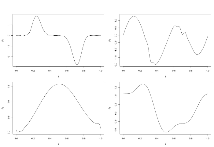
Figure 1: Slope functions of $\bm{\beta}_{1}$ to $\bm{\beta}_{4}$.

The error term $\varepsilon_{i}$ is drawn from the following distributions: 1) Standard normal : $N(0,1)$; 2) Mixed-variance: $.95N(0,1)+.05N(0,10)$; 3) t distribution with 3 degrees of freedom: $t_{3}$; 4) Standard Cauchy: $C(0,1)$. The signal-to-noise (SNR) ratio, defined as ${\mu}/{\sigma}$ in this paper, is chosen from three different levels: $\rm{SNR}=1,5,10$, where $\mu$ is the mean of signal and $\sigma$ is the standard deviation of the noise.

The sizes of the training, tuning and testing data sets are $n$, $n$ and $10n$ respectively. We select the tuning parameters via a grid search using the GIC and validation set methods through the tuning data set. In GIC, $\phi_{n}$s are $5p_{n}$, $5p_{n}$ and $p_{n}$ for the quantile sparse group lasso, lasso and group lasso methods respectively, while $p_{n}=\log\left(\log(n)\right)\log\left(\log(p)\right)/\left(10n\right)$. The validation set method is used to select the gold standard (GS) tuning parameters that minimize the prediction error of tuning data sets (Li et al., 2007, Zou and Yuan, 2008, Wu and Liu, 2009).

In our simulations, we choose $n=200$, $400$, set $\tau=0.5$, and use $100$ Monte Carlo repititions. We use the following five criteria of the performance, namely, the group accuracy (GA), variable accuracy (VA), mean absolute prediction error (MAPE), mean integrated square errors (MISE) and individual integrated square errors (ISE). The group accuracy (GA) is the proportion of correctly picked up and dropped off functional components, that is $\textrm{GA}=E\left(\left({|\widehat{M}\cap M_{0}|+|\widehat{M}^{c}\cap M_{0}^{c}|}\right)/{12}\right)$ with $M_{0}=\{l:{\beta}_{l}(t)\neq 0\}$ and $\widehat{M}=\{l:\hat{\beta}_{l}(t)\neq 0\}$. The variable accuracy (VA) is defined similarly as GA by simply replacing the $M_{0}$ and $\widehat{M}$ as the true and estimated index sets of non-zero wavelet coefficients. The mean absolute prediction error (MAPE) is MAPE$=E(|\hat{y}-y|)$. The mean integrated square errors (MISE) of the $12$ estimated functional coefficients:

$$\textrm{MISE}={\frac{1}{12}\sum_{l=1}^{12}\int_{0}^{1}(\hat{\beta}_{l}(t)-\beta_{l}(t))^{2}}dt,$$

as well as the individual integrated square error (ISE):

$$\textrm{ISE}_{l}={\int_{0}^{1}(\hat{\beta}_{l}(t)-\beta_{l}(t))^{2}}dt,$$

is used to measure the estimation accuracy of functional coefficients.

Due to space limit, we only discuss the results of SNR $=5$. The results for the other two SNRs are both in favor of our method and deferred to the Appendix. As shown in Table 1, in general, the performance of qSGL method is better than the qL and qGL methods in terms of mean integrated square errors (MISEs) and mean absolute prediction errors (MAPEs). For different error types, our proposed GIC approach is only slightly outperformed by the gold standards. As the sample size increases, the MISEs and MAPEs decrease, which is consistent with our theoretical results. For group accuracy (GA), qGL performs better than the other methods in most cases, while qL performs quite well in terms of variable accuracy (VA). However, in the case of GIC, the sparse group lasso method outperforms the two competitors regarding both GA and VA, especially for larger sample sizes. In Table 2, it shows that the ISEs of sparse group lasso are smaller than the other two methods. It also shows that the ISE of $\hat{\beta}_{1}(t)$ is always less than the other three slope functions in most cases regardless the methods used. It might be due to the fact that $\beta_{1}(t)$ is smoother than the other slopes; see Figure 1.

				GS				GIC
n	Noise	Method	MISE	GA	VA	MAPE	MISE	GA	VA	MAPE
		qSGL	1.449	0.930	0.934	2.600	1.522	0.594	0.840	2.851
	1	qL	3.230	0.919	0.961	2.871	3.159	0.482	0.904	3.205
		qGL	1.835	1.000	0.082	2.862	2.121	0.970	0.343	4.763
		qSGL	1.372	0.960	0.934	2.466	1.516	0.623	0.835	2.796
	2	qL	3.023	0.932	0.960	2.749	3.086	0.496	0.905	3.142
		qGL	1.802	1.000	0.082	2.781	2.068	0.973	0.326	4.476
200		qSGL	0.598	1.000	0.911	1.436	0.932	0.871	0.857	1.953
	3	qL	1.420	0.985	0.945	1.671	2.487	0.686	0.909	2.654
		qGL	1.630	1.000	0.065	2.386	1.735	0.993	0.140	2.836
		qSGL	1.284	0.972	0.934	2.326	1.497	0.617	0.829	2.755
	4	qL	2.826	0.927	0.958	2.625	3.135	0.490	0.907	3.145
		qGL	1.775	1.000	0.075	2.656	2.043	0.976	0.295	4.225
		qSGL	0.925	0.989	0.915	2.095	1.224	0.911	0.920	2.220
	1	qL	1.774	0.944	0.946	2.187	2.125	0.617	0.898	2.371
		qGL	1.581	1.000	0.054	2.393	2.246	0.958	0.569	5.240
		qSGL	0.842	0.995	0.911	1.954	1.105	0.967	0.937	2.058
	2	qL	1.640	0.965	0.947	2.040	1.853	0.729	0.912	2.190
		qGL	1.549	1.000	0.056	2.306	2.263	0.957	0.582	5.294
400		qSGL	0.157	1.000	0.875	1.001	0.272	1.000	0.930	1.108
	3	qL	0.285	1.000	0.908	1.026	0.481	0.991	0.943	1.108
		qGL	1.255	1.000	0.050	1.996	1.438	0.992	0.155	2.472
		qSGL	0.738	0.996	0.909	1.785	0.995	0.983	0.939	1.910
	4	qL	1.469	0.978	0.947	1.860	1.737	0.735	0.906	2.052
		qGL	1.505	0.999	0.054	2.194	2.102	0.969	0.499	4.490

Table 1: Simulation summary of SNR=5. The first column $n$ is the size of training data. The second column is the type of noise. The third column is the method we used, qSGL for the quantile sparse group lasso, qL for the quantile Lasso, and qGL for the quantile group lasso. GS means $\lambda$ was selected by the validation method (gold standard). GIC means $\lambda$ selected via the GIC criterion. MISE stands for mean integrated errors. MAPE, GA and VA indicate mean absolute prediction error, group accuracy and variable accuracy, respectively.

				GS				GIC
n	Noise	Method	ISE1	ISE2	ISE3	ISE4	ISE1	ISE2	ISE3	ISE4
		qSGL	0.116	0.585	0.331	0.385	0.133	0.550	0.322	0.387
	1	qL	0.289	0.758	1.386	0.734	0.318	0.618	1.136	0.732
		G	0.351	0.675	0.359	0.447	0.372	0.728	0.370	0.648
		qSGL	0.116	0.540	0.322	0.368	0.137	0.560	0.318	0.377
	2	qL	0.283	0.674	1.302	0.703	0.336	0.631	1.049	0.740
		qGL	0.348	0.665	0.349	0.438	0.367	0.714	0.362	0.621
200		qSGL	0.051	0.162	0.163	0.214	0.077	0.311	0.221	0.267
	3	qL	0.105	0.204	0.614	0.468	0.238	0.460	0.939	0.610
		qGL	0.332	0.605	0.297	0.395	0.342	0.632	0.313	0.446
		qSGL	0.104	0.498	0.304	0.354	0.129	0.551	0.328	0.367
	4	qL	0.248	0.628	1.211	0.679	0.318	0.613	1.157	0.707
		qGL	0.345	0.657	0.343	0.427	0.367	0.709	0.366	0.597
		qSGL	0.074	0.321	0.217	0.293	0.091	0.470	0.265	0.353
	1	qL	0.141	0.318	0.729	0.532	0.155	0.377	0.719	0.575
		qGL	0.325	0.590	0.285	0.381	0.363	0.731	0.399	0.752
		qSGL	0.071	0.274	0.207	0.273	0.088	0.421	0.248	0.331
	2	qL	0.117	0.279	0.695	0.508	0.139	0.324	0.675	0.519
		qGL	0.321	0.577	0.278	0.372	0.364	0.736	0.401	0.761
400		qSGL	0.010	0.018	0.063	0.065	0.016	0.045	0.094	0.115
	3	qL	0.012	0.017	0.139	0.110	0.018	0.034	0.234	0.187
		G	0.295	0.446	0.205	0.308	0.311	0.504	0.244	0.375
		qSGL	0.057	0.220	0.195	0.253	0.071	0.366	0.233	0.312
	4	qL	0.096	0.218	0.643	0.478	0.116	0.273	0.631	0.515
		qGL	0.319	0.555	0.266	0.363	0.354	0.700	0.383	0.664

Table 2: Individual funtional $L_{2}$ error of SNR=5. The first column n is the size of training data. The second column is the noise type. The third column is the method we used. ISE1: $||\hat{\beta}_{1}-\beta_{1}||_{2}^{2}$; ISE2: $||\hat{\beta}_{2}-\beta_{2}||_{2}^{2}$; ISE3: $||\hat{\beta}_{3}-\beta_{3}||_{2}^{2}$; ISE4: $||\hat{\beta}_{4}-\beta_{4}||_{2}^{2}$.

5.2 Real Data

The real data we use is a subset of the ADHD-200 Sample Initiative Project (Mennes et al., 2013), which studies attention deficit hyperactivity disorder (ADHD), the most commonly diagnosed mental disorder of childhood which may persist into adulthood. ADHD is characterized by problems related to paying attention, hyperactivity, or impulsive behavior. The dataset is a filtered preprocessed resting state fMRI data from New York University Child Study Centre using the Anatomical Automatic Labeling (AAL) atlas (Tzourio-Mazoyer et al., 2002). In the dataset, there are 172 equally spaced time courses in the filtering and AAL contains 116 Regions of Interests (ROIs) fractionated into functional space using nearest-neighbor interpolation. Each of 172 time courses is then smoothed to 64 equally to apply DWT. After cleaning the raw data that fails in quality control or has missing data, we have 120 individuals in final analysis. Grouping ROIs in terms of their anatomical functions and averaging within each group the corresponding time courses, we have 59 averaged time courses of grouped ROIs serving as functional predictors, each of which has 64 equally spaced time points. In addition, 8 scalar covariates are considered, including gender, age, handedness, diagnosis status, medication status, Verbal IQ, Performance IQ and Full4 IQ. The response of interest is the ADHD index, a measurement of severity of mental disorder.

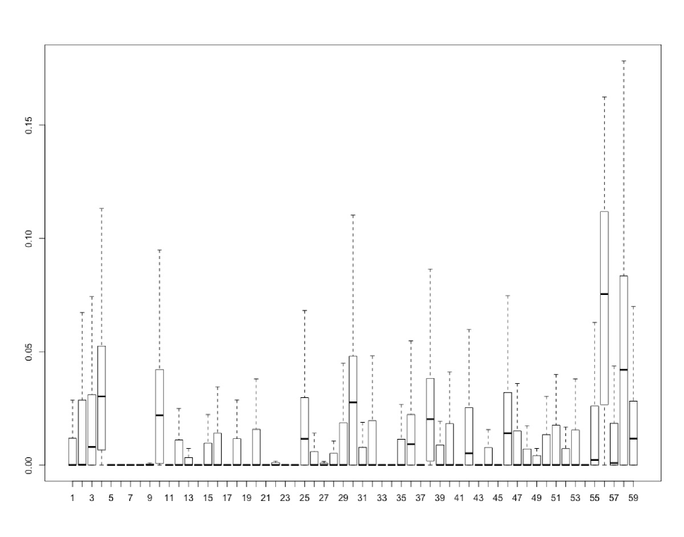
Figure 2: Boxplot of $L_{2}$ norm for each slope function, by using the quantile spare group lasso method.

We apply partial functional linear quantile regression model (4) with $59$ functional covariates and $8$ scalar covariates. In order to select the significant functional covariates from $59$ ROIs, we use the procedure proposed by Meinshausen and Bühlmann (2010) to obtain stable selections from $100$ bootstrap samples. The tuning parameters are chosen by GIC. The boxplots of $L_{2}$ norms of the estimated slope functions from bootstrap samples are shown in Figure 2, 3 and 4 in the Appendix. The selection criterion is that the median of corresponding $L_{2}$ norm should be greater than $10^{-5}$.

In neurological science literature on ADHD, it has been shown that the $7$ regions of cerebellum, temporal, vermis, parietal, occipital, cingulum and frontal are commonly discovered to be significantly related to ADHD symptoms from various studies ( Max et al., 2005; Konrad and Eickhoff, 2010; Tomasi and Volkow, 2012). We first evaluate the performances of qSGL, qL and qGL methods in terms of the selection of these 7 regions, which are essentially 14 ROIs including the left and right parts. In Table 3 and 4, we list the selected ROIs from three different methods. In particular, qSGL, qL and qGL select 15, 20 and 9 ROIs respectively. In terms of those 7/14 commonly discovered regions/ROIs, Both our proposed qSGL and qGL methods have lower false discovery rates ($33\%$) than the qL method ($55\%$), while our method is superior to the qGL as it identifies more true positives ($10$ vs $6$). Moreover, “Occipital R”, the right occipital region, can only be identified by our method. While both Table 3 and 4 confirm that most of the selected ROIs are coming from the 7/14 mostly discovered regions/ROIs, the three methods also suggest three other common ROIs: “Olfactory R”, “Supramarginal R”, and “Caudate R”, namely right olfactory, right supramarginal, and right caudate regions respectively, which have been evidently important as suggested by some ADHD studies. For instance, Schrimsher et al. (2002) revealed a relationship between caudate asymmetry and some symptoms related to ADHD. The findings of Sidlauskaite et al. (2015) imply the supramarginal gyrus is associated with the ADHD symptom scores.

Method	Significant ROIs
	“Temporal R”  “Cerebelum R”   “Frontal R”   “Occipital R”   “Olfactory R”
qSGL	“SupraMarginal R”   “Caudate R”   “Vermis”  “Cuneus L”   “Parietal R”
	“Frontal L”   “Precuneus R”   “Temporal L”   “Cerebelum L”   “Precentral R”
	“Frontal R”   “Caudate R”   “Temporal R”   “Cuneus L”   “SupraMarginal R”
	“Parietal R”   “Lingual L”   “Frontal L”   “Precuneus R”   “Vermis”
qL	“Fusiform R”   “Pallidum L”   “Olfactory R”   “Precentral R”   “Cingulum L”
	“Cuneus R”   “Parietal L”   “Temporal L”   “Angular L”   “Cerebelum R”
	“Caudate R”   “Frontal R”   “Cerebelum R”   “Vermis”   “Olfactory R”
qGL	“Temporal R”   “Precentral R”   “SupraMarginal R”   “Frontal L”

Table 3: Selected ROIs for the ADHD-200 fMRI Dataset.

Significant regions	qSGL	qL	qGL
Cerebellum	R L	R	R
Temporal	R L	R L	R
Vermis	R L	R L	R L
Parietal	R	R L
Occipital	R
Cingulum		L
Frontal	R L	L	R L

Table 4: Selected ROIs for the suggested 7 regions, ‘R’ and ‘L’ indicate the region is selected from the right brain and left brain, respectively. Blank means the brain region is not chosen.

6 Discussion

This article studies quantile regression in partial functional linear model where response is scalar and predictors include both scalars and multiple functions. We adopt wavelet basis to well approximate functional slopes while effectively detect local features. A sparse group lasso method is proposed to select important functional predictors while capture shared information among them. We reformulate the proposed problem into a standard second-order cone program and then solve it by an interior point method. A novel and efficient algorithm by using alternating direction method of multipliers (ADMM) is utilized to solve the optimization problem. In addition, we successfully derive the asymptotic properties including the convergence rate and prediction error bound which guarantee a good theoretical performance of the proposed method. Simulation studies demonstrate that our proposed method is more effective in estimating coefficients and making predictions while capable of identifying non-zero functional components and wavelet coefficients. We analyze a real data from ADHD-200 fMRI data set and show the superiority of our method. Moreover, our analysis makes some new discovery about other brain regions that are evidently important in making diagnosis.

There are several topics that merit further research. Other asymptotic properties, such as the model selection consistency and asymptotic normality, of our proposed method could be developed. The technique proposed to reformulate our problem into a second order cone program (SOCP) could be further adapted to other penalized quantile regression problems; for example, quantile ridge regression (Wu and Liu, 2009). Moreover, to estimate the functional slopes, the wavelet-based technique can also be used together with principal component analysis or partial least squares methods (Reiss et al., 2015).

7 Appendix

				GS				GIC
n	Noise	Method	MISE	GA	VA	MAPE	MISE	GA	VA	MAPE
		qSGL	2.426	0.860	0.959	9.557	6.361	0.480	0.854	11.720
	1	qL	5.885	0.965	0.972	9.553	17.062	0.358	0.891	13.134
		qGL	2.601	0.852	0.118	9.637	4.091	0.708	0.406	12.728
		qSGL	2.322	0.876	0.958	8.833	6.013	0.509	0.857	10.968
	2	qL	5.592	0.968	0.971	8.844	16.564	0.363	0.891	12.760
		qGL	2.619	0.870	0.123	8.973	4.473	0.704	0.374	11.844
200		qSGL	1.063	0.994	0.930	4.200	1.594	0.891	0.908	4.774
	3	qL	2.462	0.978	0.958	4.491	7.252	0.547	0.911	7.466
		qGL	1.741	1.000	0.073	4.776	3.699	0.857	0.330	7.875
		qSGL	2.252	0.925	0.958	7.967	5.795	0.510	0.856	10.353
	4	qL	5.332	0.983	0.971	8.012	15.874	0.365	0.891	12.401
		qGL	2.402	0.920	0.113	8.099	4.152	0.751	0.404	11.165
		qSGL	2.186	0.935	0.954	8.699	2.427	0.959	0.974	9.529
	1	qL	5.246	0.981	0.971	8.756	5.916	0.966	0.970	8.906
		qGL	2.336	0.944	0.106	8.788	3.450	0.877	0.667	11.703
		qSGL	2.126	0.954	0.954	8.083	2.414	0.963	0.976	9.030
	2	qL	4.962	0.983	0.970	8.153	5.175	1.000	0.974	8.206
		qGL	2.234	0.973	0.102	8.182	2.742	0.898	0.718	11.403
400		qSGL	0.492	1.000	0.883	3.630	1.004	0.999	0.951	3.985
	3	qL	1.035	0.995	0.934	3.698	1.855	0.994	0.965	4.018
		qGL	1.415	1.000	0.052	4.305	2.394	0.932	0.551	7.679
		qSGL	2.008	0.962	0.950	7.301	2.338	0.965	0.975	8.258
	4	qL	4.602	0.983	0.970	7.394	5.991	0.967	0.968	7.634
		qGL	2.133	0.983	0.102	7.376	3.250	0.888	0.692	10.880

Table 5: Simulation summary of SNR=1, as for Table 1.

				GS				GIC
n	Noise	Method	ISE1	ISE2	ISE3	ISE4	ISE1	ISE2	ISE3	ISE4
		qSGL	0.186	0.822	0.673	0.684	0.270	2.415	0.749	0.654
	1	qL	0.629	1.004	3.197	0.987	1.073	3.883	3.019	2.129
		qGL	0.407	0.901	0.537	0.693	0.529	1.851	0.555	0.868
		qSGL	0.181	0.810	0.642	0.635	0.264	2.494	0.712	0.640
	2	qL	0.592	0.973	2.974	0.989	1.078	4.370	2.808	1.825
		qGL	0.411	0.971	0.521	0.660	0.530	2.198	0.583	0.861
200		qSGL	0.087	0.394	0.252	0.315	0.112	0.646	0.322	0.383
	3	qL	0.197	0.520	1.067	0.640	0.575	1.677	1.619	1.045
		qGL	0.342	0.645	0.330	0.422	0.438	1.729	0.497	0.737
		qSGL	0.165	0.816	0.646	0.589	0.243	2.383	0.764	0.641
	4	qL	0.552	0.961	2.781	0.986	0.982	4.010	2.891	1.769
		qGL	0.396	0.858	0.511	0.605	0.509	1.989	0.544	0.862
		qSGL	0.163	0.830	0.593	0.565	0.189	0.801	0.616	0.817
	1	qL	0.565	0.973	2.692	0.966	0.549	1.176	2.773	1.060
		qGL	0.387	0.837	0.492	0.598	0.453	1.339	0.422	1.041
		qSGL	0.165	0.814	0.579	0.540	0.194	0.795	0.619	0.803
	2	qL	0.513	0.966	2.501	0.938	0.523	0.970	2.679	0.982
		qGL	0.383	0.797	0.476	0.563	0.420	0.900	0.375	1.007
400		qSGL	0.038	0.133	0.137	0.177	0.070	0.393	0.241	0.298
	3	qL	0.065	0.147	0.456	0.350	0.123	0.404	0.814	0.500
		qGL	0.312	0.516	0.242	0.344	0.383	0.778	0.405	0.802
		qSGL	0.146	0.794	0.540	0.502	0.176	0.799	0.604	0.758
	4	qL	0.414	0.952	2.281	0.919	0.461	1.269	2.478	1.140
		qGL	0.376	0.771	0.448	0.527	0.433	1.177	0.412	1.041

Table 6: Individual funtional $L_{2}$ error when SNR=1, as for Table 2.

				GS				GIC
n	Noise	Method	MISE	GA	VA	MAPE	MISE	GA	VA	MAPE
		qSGL	0.907	0.988	0.906	1.617	0.920	0.935	0.839	1.683
	1	qL	1.962	0.917	0.939	1.835	1.964	0.792	0.910	1.917
		qGL	1.679	1.000	0.064	2.195	1.743	0.994	0.132	2.578
		qSGL	0.898	0.992	0.912	1.576	0.913	0.943	0.840	1.662
	2	qL	1.866	0.932	0.942	1.784	1.917	0.790	0.912	1.888
		qGL	1.669	1.000	0.067	2.172	1.779	0.989	0.161	2.857
200		qSGL	0.498	1.000	0.903	1.124	0.709	0.943	0.849	1.482
	3	qL	1.203	0.993	0.943	1.325	1.756	0.828	0.914	1.867
		qGL	1.603	1.000	0.062	2.170	1.659	0.995	0.109	2.465
		qSGL	0.842	0.992	0.915	1.502	0.911	0.943	0.843	1.656
	4	qL	1.774	0.952	0.944	1.709	1.928	0.792	0.913	1.904
		qGL	1.656	1.000	0.065	2.116	1.722	0.996	0.125	2.420
		qSGL	0.499	0.999	0.892	1.142	0.610	0.963	0.874	1.222
	1	qL	0.981	0.965	0.932	1.187	1.029	0.838	0.879	1.278
		qGL	1.371	1.000	0.051	1.684	1.557	0.998	0.208	2.183
		qSGL	0.458	1.000	0.890	1.069	0.565	0.981	0.897	1.145
	2	qL	0.902	0.975	0.933	1.114	0.927	0.867	0.894	1.190
		qGL	1.361	1.000	0.052	1.665	1.567	0.996	0.216	2.275
400		qSGL	0.096	1.000	0.874	0.602	0.167	1.000	0.918	0.671
	3	qL	0.151	1.000	0.903	0.617	0.299	0.999	0.941	0.681
		qGL	1.220	1.000	0.050	1.679	1.260	1.000	0.081	1.759
		qSGL	0.410	1.000	0.891	0.981	0.515	0.978	0.899	1.067
	4	qL	0.837	0.988	0.934	1.025	0.866	0.898	0.898	1.105
		qGL	1.336	1.000	0.050	1.627	1.494	0.997	0.175	2.075

Table 7: Simulation summary of SNR=10, as for Table 1.

				GS				GIC
n	Noise	Method	ISE1	ISE2	ISE3	ISE4	ISE1	ISE2	ISE3	ISE4
		qSGL	0.080	0.298	0.220	0.286	0.082	0.292	0.222	0.284
	1	qL	0.166	0.340	0.819	0.570	0.165	0.317	0.799	0.569
		qGL	0.334	0.625	0.312	0.407	0.338	0.637	0.318	0.449
		qSGL	0.081	0.299	0.216	0.282	0.087	0.294	0.218	0.277
	2	qL	0.158	0.315	0.776	0.559	0.177	0.321	0.746	0.565
		qGL	0.334	0.621	0.310	0.403	0.342	0.641	0.318	0.477
200		qSGL	0.040	0.117	0.146	0.188	0.061	0.206	0.182	0.233
	3	qL	0.077	0.148	0.540	0.415	0.141	0.265	0.737	0.512
		qGL	0.330	0.597	0.289	0.387	0.333	0.607	0.296	0.423
		qSGL	0.072	0.270	0.211	0.271	0.080	0.293	0.227	0.273
	4	qL	0.137	0.293	0.751	0.543	0.171	0.308	0.788	0.549
		qGL	0.333	0.618	0.306	0.397	0.337	0.630	0.319	0.435
		qSGL	0.038	0.119	0.145	0.188	0.050	0.164	0.156	0.214
	1	qL	0.052	0.109	0.440	0.349	0.056	0.119	0.415	0.334
		qGL	0.307	0.501	0.229	0.333	0.316	0.562	0.279	0.400
		qSGL	0.036	0.100	0.141	0.173	0.046	0.146	0.157	0.202
	2	qL	0.044	0.094	0.412	0.327	0.050	0.099	0.385	0.309
		qGL	0.305	0.498	0.227	0.330	0.316	0.560	0.278	0.413
400		qSGL	0.005	0.007	0.043	0.040	0.008	0.017	0.069	0.072
	3	qL	0.007	0.007	0.076	0.059	0.009	0.013	0.154	0.121
		qGL	0.291	0.430	0.198	0.301	0.294	0.445	0.209	0.312
		Q	0.028	0.080	0.135	0.160	0.038	0.122	0.150	0.191
	4	qL	0.039	0.076	0.397	0.306	0.043	0.085	0.380	0.294
		qGL	0.302	0.485	0.223	0.325	0.311	0.532	0.263	0.388

Table 8: Individual funtional $L_{2}$ error when SNR=10, as for Table 2.

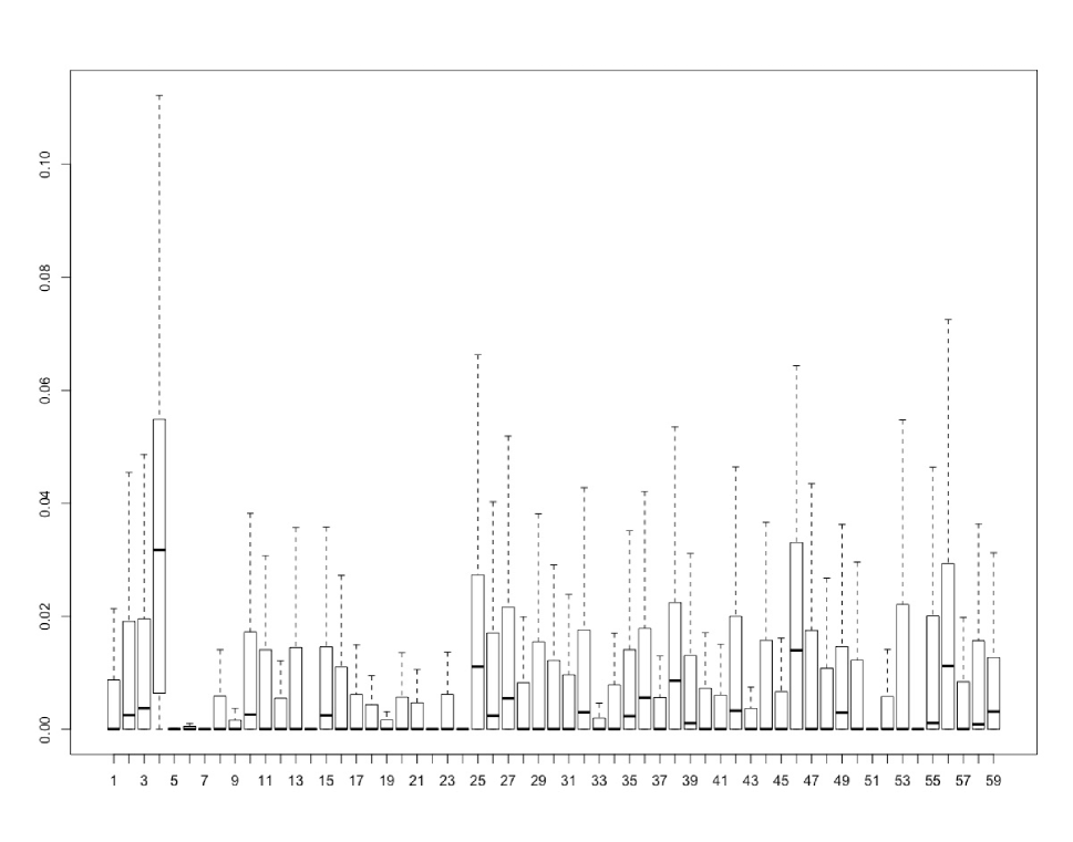
Figure 3: Boxplot of $L_{2}$ norm for each slope function, by using the quantile lasso method.

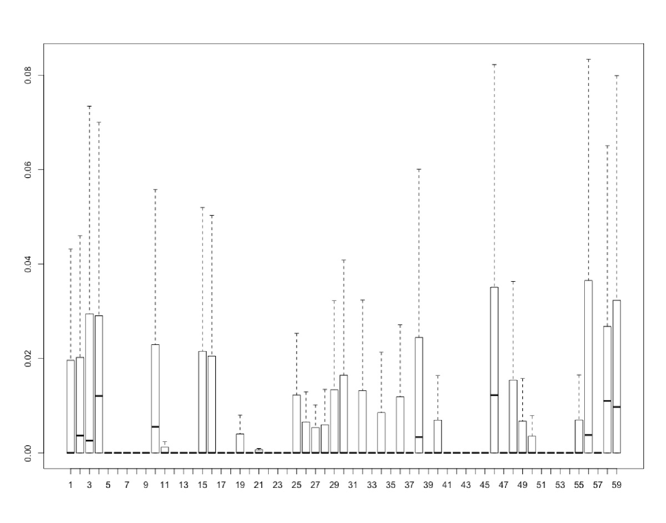
Figure 4: Boxplot of $L_{2}$ norm for each slope function, by using the quantile group lasso method.

7.1 Proof of Theorem 1

Proof.

First, we introduce some notation. The orthonormal wavelet basis set of $L^{2}[0,1]$ is defined as $\{\varphi_{j_{0}k},k=1,\dots,2^{j_{0}}\}\cup\{\psi_{jk},\ j\geq j_{0},\ k=1,\dots,2^{j}\}$. Without loss of generality, the wavelet basis are ordered according to the scales from the coarsest level $J_{0}$ to the finest one. Let $\mathbb{V}_{N_{n}}:=\textrm{Span}\{\bm{\varphi}_{1},\ \dots,\ \bm{\varphi}_{N_{n}}\}$ be the space spanned by the first $N_{n}$ basis function, for example, if $N_{n}=2^{j_{0}+t}$, then the collection of $\{\varphi_{j_{0}k},k=1\dots,2^{j_{0}}\}\cup\{\psi_{jk},j_{0}\leq j\leq j_{0}+t-1,\ k=1,\dots,\ 2^{j}\}$ is the basis of $\mathbb{V}_{N_{n}}$. Let $\bm{b}_{N_{n}}^{j}$ be an $N_{n}\times 1$ parameter vector with elements $b_{k}^{j}=\langle\beta_{j}(t),\varphi_{k}\rangle$. In addition, let $\beta_{N_{n}}^{j}$ be the functions reconstructed from the vector $\bm{b}_{N_{n}}^{j}$. Here $\beta_{N_{n}}^{j}$ is a linear approximation to $\beta_{j}$ by the first $N_{n}$ wavelet coefficients, while $\hat{\beta}_{j}$ denotes the function reconstructed from the wavelet coefficients $\hat{\bm{b}}_{j}$ from (10).

By the Parseval theorem, we have $||\hat{\beta}_{j}-\beta_{j}||_{L_{2}}^{2}=||\hat{b}^{j}_{N_{n}}-b^{j}_{N_{n}}||_{2}^{2}+\sum_{k={N_{n}}+1}^{\infty}{\theta_{k}^{j}}^{2}$. To derive the convergence rate of $\hat{\beta_{j}}$ to $\beta_{j}$, we bound the error in estimating $\beta_{N_{n}}^{j}$ by $\hat{\beta_{j}}$ and the error in approximating $\beta_{j}$ by $\beta_{N_{n}}$. By the Theorem 9.5 of Mallat (2008), the linear approximation error goes to zero as

$$\sum_{k={N_{n}}+1}^{\infty}{b_{k}^{j}}^{2}=o(N_{n}^{-2d}).$$ (16)

Let $\Upsilon^{0}=(\bm{\alpha}^{0},\bm{\gamma}^{0},\bm{\theta}^{0})$ be the true coefficients with $\bm{\theta}^{0}=\rm{vec}^{T}\left(\bm{b}_{N_{n}}^{1},\dots,\bm{b}_{N_{n}}^{m}\right)$. To obtain the result, we show that for any given $\varepsilon>0$, there exists a constant $C$ such that

$$\textrm{Pr}\left\{\inf_{||\bm{z}||=C}L_{n}\left(\Upsilon^{0}+r_{n}\bm{z}\right)+P_{\lambda_{1},\lambda_{2}}\left(\bm{\theta}^{0}+r_{n}\bm{z}_{\theta}\right)>L_{n}\left(\Upsilon^{0}\right)+P_{\lambda_{1},\lambda_{2}}\left(\bm{\theta}^{0}\right)\right\}\geq 1-\varepsilon,$$ (17)

where $r_{n}=\sqrt{{N_{n}}/{n}}$ and $\bm{z}=(z_{1},\dots,z_{k},\bm{z}_{\bm{\gamma}},\bm{z}_{\bm{\theta}})$ is a vector with the same length of vector $\Upsilon^{0}$. This implies that there exists a local minimizer in the ball $\{\Upsilon^{0}+r_{n}z:||z||\leq C\}$ with probability at least $1-\varepsilon$. Hence, there is a local minimizer $\widehat{\Upsilon}$ such that $||\widehat{\Upsilon}-\Upsilon^{0}||=O_{p}(r_{n})$.

To show (17), we compare $L_{n}(\bm{\Upsilon}^{0})+P_{n}(\bm{\theta}^{0})$ with $L_{n}(\bm{\Upsilon}^{0}+r_{n}\bm{z})+P_{n}(\theta^{0}+r_{n}\bm{z}_{\theta})$. By using the Knight identity,

$$\rho_{\tau}(u-v)-\rho_{\tau}(u)=-v\varrho_{\tau}(u)+\int_{0}^{v}(I(u\leq t)-I(u\leq 0))dt,$$

where $\varrho_{\tau}(u)=\tau-I(u<0)$, we have

$$I := L_{n}(\bm{\Upsilon}^{0}+r_{n}\bm{v})-L_{n}(\bm{\Upsilon}^{0})$$

$$= \sum_{k=1}^{K}\sum_{i=1}^{n}[{\rho}_{\tau_{k}}(e_{ki}-d_{ki})-{\rho}_{\tau_{k}}(e_{ki})]$$

$$= -\sum_{k=1}^{K}\sum_{i=1}^{n}[-d_{ki}\varrho_{\tau_{k}}(e_{ki})]+\sum_{k=1}^{K}\sum_{i=1}^{n}\int_{0}^{d_{ki}}(I(e_{ki}\leq t)-I(e_{ki}\leq 0))dt$$

$$= I_{1}+I_{2},$$

where $e_{ki}=y_{i}-\alpha_{\tau_{k}}^{0}-\bm{u}_{i}^{T}\bm{\gamma}^{0}-\bm{v}_{i}^{T}\bm{\theta}^{0}$ and $b_{ki}=r_{n}z_{k}+r_{n}\bm{u}_{i}^{T}\bm{z}_{u}+r_{n}\bm{v}_{i}^{T}\bm{z}_{\theta}$. Note that $e_{ki}=\varepsilon_{i}-F^{-1}(\tau_{k})+o(N_{n}^{-2d})$, hence we have $E(\varrho_{\tau_{k}}(e_{ki})=o(N_{n}^{-2d})$. By the definition of $d_{ki}$, we obtain $I_{1}\leq{r_{n}}||\bm{z}||(\sum_{k=1}^{s}||\sum_{i=1}^{n}\varrho_{\tau_{k}}(e_{ki})\bm{A}_{i}^{T}||)$ and

$$E||\sum_{i=1}^{n}\varrho_{\tau_{k}}(e_{ki})\bm{A}_{i}||^{2} = E||\sum_{j=1}^{mN_{n}+1}\sum_{i=1}^{n}\sum_{l=1}^{n}a_{ij}a_{lj}\psi_{\tau_{k}}(e_{ki})\psi_{\tau_{k}}(e_{kl})||$$

$$= O_{p}(nN_{n}),$$

which leads to $E(I_{1})\leq O_{p}({r_{n}}\sqrt{nN_{n}})||\bm{z}||=O_{p}(nr_{n}^{2})||\bm{z}||$.

Now, we consider the expectation of $I_{2}$. Using the expression of $e_{ki}$, we get

$$E(I_{2}) = \sum_{k=1}^{K}\sum_{i=1}^{n}\int_{0}^{d_{ki}}(\textrm{Pr}(e_{ki}\leq t)-\textrm{Pr}(e_{ki}\leq 0))dt$$

$$= \sum_{k=1}^{K}\sum_{i=1}^{n}\int_{0}^{d_{ki}}(F(F^{-1}(\tau_{k})+o(N_{n}^{-2d})+t)-F(F^{-1}(\tau_{k})+o(N_{n}^{-2d})))dt$$

$$= \sum_{k=1}^{K}\sum_{i=1}^{n}\int_{0}^{d_{ki}}(f(F^{-1}(\tau_{k})+o(N_{n}^{-2d}))t+\frac{f^{\prime}(\xi)}{2}t^{2})dt,$$

where $\xi$ lies between $F^{-1}(\tau_{k})+o(N_{n}^{-2d})$ and $F^{-1}(\tau_{k})+o(N_{n}^{-2d})+d_{ki}$. Since there exists $M$ such that $||A_{i}||_{2}^{2}<M$, we have

$$\max_{1\leq i\leq n}|r_{n}z_{k}+r_{n}\bm{v}_{i}^{T}\bm{z}_{\theta}|\to 0.$$

Then, the lower bound of $E(I_{2})$ is of the form

$$E(I_{2}) = \frac{1}{2}r_{n}^{2}\sum_{k=1}^{K}\{[f(F^{-1}(\tau_{k})+o(N_{n}^{-2d}))+o_{p}(1)](\bm{g}_{k}^{T}A^{T}A\bm{g}_{k})\}$$

$$\geq \frac{c_{1}nr_{n}^{2}}{2}||\bm{z}||^{2}_{2}\min_{k}\{f(F^{-1}(\tau_{k})+o(N_{n}^{-2d}))+o_{p}(1)\},$$

where $\bm{g}_{k}$ is a vector, such as $\bm{g}_{k}=(z_{k},\bm{z}_{\theta}^{T},\bm{z}_{u}^{T})^{T}$. Finally, since $r_{n}\to 0$ and $||\bm{z}||_{2}\leq C$, we have

$$II:=P_{n}(\theta^{0}+r_{n}\bm{z}_{\theta})-P_{n}(\theta^{0}) \leq \lambda_{1}r_{n}||\bm{z}_{\theta}||_{1}+\lambda_{2}r_{n}\sum_{j=1}^{m}||\bm{z}_{\theta_{j}}||_{2}$$

$$\leq \lambda_{1}r_{n}\sqrt{mN}||\bm{z}_{\theta}||_{2}+\lambda_{2}r_{n}m||\bm{z}_{\theta}||_{2}$$

$$= O_{p}(nr_{n}^{2}||\bm{z}_{\theta}||_{2}).$$

Since $II$ is bounded by $r_{n}^{2}||\bm{z}_{\theta}||_{2}$ ,we can choose a $C$ such that the II is dominated by the term $I_{2}$ on $||u||=C$ uniformly. So $Q_{n}(\Sigma^{0}+r_{n}u)-Q_{n}(\Sigma^{0})>0$ holds uniformly on $||u||=C$. This completes the proof. ∎

References

- Antoniadis et al. (2001) Antoniadis, A., J. Bigot, and T. Sapatinas (2001). Wavelet estimators in nonparametric regression: a comparative simulation study. Journal of Statistical Software 6, pp–1.
- Aps (2015) Aps, M. (2015). Rmosek: The r to mosek optimization interface. URL http://rmosek. r-forge. r-project. org/, http://www. mosek. com/. R package version 7(2).
- Boyd et al. (2011) Boyd, S., N. Parikh, E. Chu, B. Peleato, and J. Eckstein (2011). Distributed optimization and statistical learning via the alternating direction method of multipliers. Foundations and Trends® in Machine Learning 3(1), 1–122.
- Bradic et al. (2011) Bradic, J., J. Fan, and W. Wang (2011). Penalized composite quasi-likelihood for ultrahigh dimensional variable selection. Journal of the Royal Statistical Society: Series B (Statistical Methodology) 73(3), 325–349.
- Cai and Hall (2006) Cai, T. T. and P. Hall (2006). Prediction in functional linear regression. The Annals of Statistics 34(5), 2159–2179.
- Cardot et al. (2005) Cardot, H., C. Crambes, and P. Sarda (2005). Quantile regression when the covariates are functions. Nonparametric Statistics 17(7), 841–856.
- Cardot et al. (1999) Cardot, H., F. Ferraty, and P. Sarda (1999). Functional linear model. Statistics and Probability Letters 45(1), 11 – 22.
- Cardot et al. (2003) Cardot, H., F. Ferraty, and P. Sarda (2003). Spline estimators for the functional linear model. Statistica Sinica 13(3), 571–592.
- Collazos et al. (2016) Collazos, J. A., R. Dias, and A. Z. Zambom (2016). Consistent variable selection for functional regression models. Journal of Multivariate Analysis 146, 63–71.
- Daubechies (1990) Daubechies, I. (1990). The wavelet transform, time-frequency localization and signal analysis. IEEE transactions on information theory 36(5), 961–1005.
- Delaigle and Hall (2012) Delaigle, A. and P. Hall (2012). Methodology and theory for partial least squares applied to functional data. The Annals of Statistics 40(1), 322–352.
- Donoho and Johnstone (1994) Donoho, D. L. and J. M. Johnstone (1994). Ideal spatial adaptation by wavelet shrinkage. Biometrika 81(3), 425–455.
- Fan and Lv (2010) Fan, J. and J. Lv (2010). A selective overview of variable selection in high dimensional feature space. Statistica Sinica 20(1), 101.
- Gabay and Mercier (1976) Gabay, D. and B. Mercier (1976). A dual algorithm for the solution of nonlinear variational problems via finite element approximation. Computers & Mathematics with Applications 2(1), 17–40.
- Gao and Kong (2015) Gao, J. and L. Kong (2015). Quantile, composite quantile regression and regularized versions [r package cqrreg version 1.2].
- Gertheiss et al. (2013) Gertheiss, J., A. Maity, and A.-M. Staicu (2013). Variable selection in generalized functional linear models. Stat 2(1), 86–101.
- Hestenes (1969) Hestenes, M. R. (1969). Multiplier and gradient methods. Journal of optimization theory and applications 4(5), 303–320.
- Kai et al. (2010) Kai, B., R. Li, and H. Zou (2010). Local composite quantile regression smoothing: an efficient and safe alternative to local polynomial regression. Journal of the Royal Statistical Society: Series B (Statistical Methodology) 72(1), 49–69.
- Kai et al. (2011) Kai, B., R. Li, and H. Zou (2011). New efficient estimation and variable selection methods for semiparametric varying-coefficient partially linear models. Annals of statistics 39(1), 305.
- Kato (2012) Kato, K. (2012). Estimation in functional linear quantile regression. Annals of Statistics 40(6), 3108–3136.
- Koenker (2005) Koenker, R. (2005). Quantile regression. Cambridge university press.
- Koenker and Bassett (1978) Koenker, R. and G. Bassett (1978). Regression quantiles. Econometrica: journal of the Econometric Society 46(1), 33–50.
- Koenker and Park (1996) Koenker, R. and B. J. Park (1996). An interior point algorithm for nonlinear quantile regression. Journal of Econometrics 71(1), 265–283.
- Kong et al. (2016) Kong, D., K. Xue, F. Yao, and H. H. Zhang (2016). Partially functional linear regression in high dimensions. Biometrika, asv062.
- Kong et al. (2015) Kong, L., H. Shu, G. Heo, and Q. C. He (2015). Estimation for bivariate quantile varying coefficient model. arXiv preprint arXiv:1511.02552.
- Konrad and Eickhoff (2010) Konrad, K. and S. B. Eickhoff (2010). Is the adhd brain wired differently? a review on structural and functional connectivity in attention deficit hyperactivity disorder. Human brain mapping 31(6), 904–916.
- Li et al. (2007) Li, Y., Y. Liu, and J. Zhu (2007). Quantile regression in reproducing kernel hilbert spaces. Journal of the American Statistical Association 102(477), 255–268.
- Lian (2013) Lian, H. (2013). Shrinkage estimation and selection for multiple functional regression. Statistica Sinica, 51–74.
- Lin et al. (2013) Lin, C.-Y., H. Bondell, H. H. Zhang, and H. Zou (2013). Variable selection for non-parametric quantile regression via smoothing spline analysis of variance. Stat 2(1), 255–268.
- Lobo et al. (1998) Lobo, M. S., L. Vandenberghe, S. Boyd, and H. Lebret (1998). Applications of second-order cone programming. Linear algebra and its applications 284(1-3), 193–228.
- Lu et al. (2014) Lu, Y., J. Du, and Z. Sun (2014). Functional partially linear quantile regression model. Metrika 77(2), 317–332.
- Mallat (2008) Mallat, S. (2008). A Wavelet Tour of Signal Processing, Third Edition: The Sparse Way (3rd ed.). Academic Press.
- Max et al. (2005) Max, J. E., F. F. Manes, B. A. Robertson, K. Mathews, P. T. Fox, and J. Lancaster (2005). Prefrontal and executive attention network lesions and the development of attention-deficit/hyperactivity symptomatology. Journal of the American Academy of Child & Adolescent Psychiatry 44(5), 443–450.
- Meinshausen and Bühlmann (2010) Meinshausen, N. and P. Bühlmann (2010). Stability selection. Journal of the Royal Statistical Society: Series B (Statistical Methodology) 72(4).
- Mennes et al. (2013) Mennes, M., B. B. Biswal, F. X. Castellanos, and M. P. Milham (2013). Making data sharing work: the fcp/indi experience. Neuroimage 82, 683–691.
- Morris (2015) Morris, J. S. (2015). Functional regression. Annual Review of Statistics and its Applications 2.
- Müller and Yao (2008) Müller, H.-G. and F. Yao (2008). Functional additive models. Journal of the American Statistical Association 103(484), 1534–1544.
- Ramsay (2006) Ramsay, J. O. (2006). Functional data analysis. Wiley Online Library.
- Reiss et al. (2015) Reiss, P. T., L. Huo, Y. Zhao, C. Kelly, and R. T. Ogden (2015). Wavelet-domain regression and predictive inference in psychiatric neuroimaging. The annals of applied statistics 9(2), 1076.
- Schrimsher et al. (2002) Schrimsher, G. W., R. L. Billingsley, E. F. Jackson, and B. D. Moore (2002). Caudate nucleus volume asymmetry predicts attention-deficit hyperactivity disorder (ADHD) symptomatology in children. Journal of Child Neurology 17(12), 877–884.
- Sidlauskaite et al. (2015) Sidlauskaite, J., K. Caeyenberghs, E. Sonuga-Barke, H. Roeyers, and J. R. Wiersema (2015). Whole-brain structural topology in adult attention-deficit/hyperactivity disorder: Preserved global - disturbed local network organization. NeuroImage: Clinical 9, 506 – 512.
- Simon et al. (2013) Simon, N., J. Friedman, T. Hastie, and R. Tibshirani (2013). A sparse-group lasso. Journal of Computational and Graphical Statistics 22(2), 231–245.
- Sun (2005) Sun, Y. (2005). Semiparametric efficient estimation of partially linear quantile regression models. Annals of Economics and Finance 6(1), 105.
- Tang and Cheng (2014) Tang, Q. and L. Cheng (2014). Partial functional linear quantile regression. Science China Mathematics 57(12), 2589–2608.
- Tomasi and Volkow (2012) Tomasi, D. and N. D. Volkow (2012). Abnormal functional connectivity in children with attention-deficit/hyperactivity disorder. Biological psychiatry 71(5), 443–450.
- Tzourio-Mazoyer et al. (2002) Tzourio-Mazoyer, N., B. Landeau, D. Papathanassiou, F. Crivello, O. Etard, N. Delcroix, B. Mazoyer, and M. Joliot (2002). Automated anatomical labeling of activations in SPM using a macroscopic anatomical parcellation of the MNI MRI single-subject brain. Neuroimage 15(1), 273–289.
- Wang et al. (2015) Wang, J.-L., J.-M. Chiou, and H.-G. Müller (2015). Review of functional data analysis. Annual Review of Statistics and its Applications 1, 41.
- Wang et al. (2014) Wang, X., B. Nan, J. Zhu, and R. Koeppe (2014). Regularized 3D functional regression for brain image data via haar wavelets. The Annals of Applied Statistics 8(2), 1045.
- Wu and Liu (2009) Wu, Y. and Y. Liu (2009). Variable selection in quantile regression. Statistica Sinica 19(2), 801.
- Yao et al. (2017) Yao, F., S. Sue-Chee, and F. Wang (2017). Regularized partially functional quantile regression. Journal of Multivariate Analysis 156, 39–56.
- Yu et al. (2016) Yu, D., L. Kong, and I. Mizera (2016). Partial functional linear quantile regression for neuroimaging data analysis. Neurocomputing 195, 74–87.
- Zhang et al. (2010) Zhang, Y., R. Li, and C.-L. Tsai (2010). Regularization parameter selections via generalized information criterion. Journal of the American Statistical Association 105(489), 312–323.
- Zhao et al. (2014) Zhao, W., R. Zhang, and J. Liu (2014). Sparse group variable selection based on quantile hierarchical lasso. Journal of Applied Statistics 41(8), 1658–1677.
- Zhao et al. (2015) Zhao, Y., H. Chen, and R. T. Ogden (2015). Wavelet-based weighted lasso and screening approaches in functional linear regression. Journal of Computational and Graphical Statistics 24(3), 655–675.
- Zhao et al. (2012) Zhao, Y., R. T. Ogden, and P. T. Reiss (2012). Wavelet-based lasso in functional linear regression. Journal of Computational and Graphical Statistics 21(3), 600–617.
- Zheng et al. (2015) Zheng, Q., L. Peng, and X. He (2015). Globally adaptive quantile regression with ultra-high dimensional data. Annals of Statistics 43(5), 2225.
- Zou and Yuan (2008) Zou, H. and M. Yuan (2008). Composite quantile regression and the oracle model selection theory. Annals of Statistics 36(3), 1108–1126.