Resampling Strategy in Sequential Monte Carlo for Constrained Sampling Problems

Abstract

Sequential Monte Carlo (SMC) methods are a class of Monte Carlo methods that are used to obtain random samples of a high dimensional random variable in a sequential fashion. Many problems encountered in applications often involve different types of constraints. These constraints can make the problem much more challenging. In this paper, we formulate a general framework of using SMC for constrained sampling problems based on forward and backward pilot resampling strategies. We review some existing methods under the framework and develop several new algorithms. It is noted that all information observed or imposed on the underlying system can be viewed as constraints. Hence the approach outlined in this paper can be useful in many applications.

Keywords: Backward sampling, Constrained sampling, Pilot, Priority score, Resampling, Sequential Monte Carlo

1 Introduction

Stochastic dynamic systems are used to model the dynamic behavior of random variables in a wide range of applications in physics, finance, engineering and other fields. One of the important problems of studying complex dynamic systems is to sample paths following the underlying stochastic process. Such paths can be used for statistical inferences under the Monte Carlo framework. In practice, a stochastic system often comes with observable information, including direct/indirect measurements, external constraints and others. For example, in a state-space model, noisy measurements of the underlying latent states are observed. In a diffusion bridge sampling problem, the start and end points of the diffusion process are fixed. In this paper, we take the view that the underlying system is given and all available information is treated as imposed constraints.

The Sequential Monte Carlo (SMC) methods are a class of sampling methods that utilize the sequential nature of the underlying process. It has a wide range of applications (Kong et al., 1994; Avitzour, 1995; Liu and Chen, 1995; Kitagawa, 1996; Kim et al., 1998; Pitt and Shephard, 1999; Chen et al., 2000; Doucet et al., 2001; Fong et al., 2002; Godsill et al., 2004). The sequential importance sampling with resampling (SISR) scheme embedded in SMC enables sampling from complex target distributions (Gordon et al., 1993; Kong et al., 1994; Liu and Chen, 1998). However, the choice of proposal distribution and the choice of priority score for resampling in SISR are crucial to sample quality and inference efficiency. For example, in a diffusion bridge sampling problem, where the start and end points of a diffusion process are exactly enforced, Pedersen (1995) proposed to generate the samples through the underlying diffusion process without considering the endpoint constraint and then force the samples to connect with the fixed point at the end. It may not be efficient due to the large deviation of the end of the forward paths from the enforced end point. Durham and Gallant (2002) proposed a method based on SMC with linear interpolation as the proposal distribution. It ignores the drift term of the underlying diffusion process and may not be efficient for non-linear processes. Lin et al. (2010) generated bridge samples based on a backward pilot resampling strategy. In their procedure, a pilot run is conducted backward from the fixed end point to determine the priority scores for resampling in a forward SISR procedure. The backward pilot resampling strategy achieves good efficiency. This approach improves the forward sampling by bringing future information and constraints for effective sampling, especially with minimum additional computational costs.

In this article, we extend the procedure of Lin et al. (2010) to more general settings. Specifically, the problem of simulating a stochastic process under constraints is more formally stated in a general setting that contains many problems as its special cases, including the standard state space models. The general setting also allows the discussion of a formal guidance for improving efficiency in developing SMC implementations for such problems. Under the setting, we propose a general framework for constrained sampling problems with measure theoretic interpretations. Resampling strategies based on forward pilots and backward pilots are developed under such a framework. Several types of constraints are discussed along with their corresponding SMC implementations. Links to the existing procedures are also discussed. The developed approaches are demonstrated with several examples.

The rest of this paper is organized as follows. In Section 2, the constrained sampling problem is formally stated and a general framework of the constrained SMC (cSMC) method is proposed. Section 3 introduces some special constrained problems with their corresponding implementations under the cSMC framework. Section 4 presents several methods to estimate the priority scores used in the resampling step of cSMC. Three examples are used to demonstrate performance of the proposed methods in Section 5. Section 6 concludes.

2 Constrained Sampling Problems

2.1 Stochastic Dynamic System with Constraints

The stochastic system we consider contains a sequence of unobservable random states $x_{0:T}=\{x_{0},x_{1},\cdots,x_{T}\}$, whose dynamics is governed by an initial state distribution $p(x_{0})$ and a known forward propagation distribution $p(x_{t}\,|\,x_{0:t-1})$. In addition, a compounded information/constraint set $\mathcal{I}_{0:T}$ imposed on the latent states is given, where $\mathcal{I}_{0:T}=\mathcal{I}_{0}\cap\mathcal{I}_{1}\cap\cdots\cap\mathcal{I}_{T}$ and $\mathcal{I}_{t}$ is the new available information at time $t$. For example, if we have a noisy measurement $y_{t}=g(x_{t},\varepsilon_{t})$ at time $t$, then $\mathcal{I}_{t}=\{y_{t}\}$. If $x_{t}$ is a fixed point via prior knowledge or design, we have $\mathcal{I}_{t}=\{x_{t}=c\}$. When there is no additional information at time $t$, we define $\mathcal{I}_{t}=\{x_{t}\in\mathcal{X}\}$, a trivial constraint, where $\mathcal{X}$ is the support of the state variable. We further assume that

$$p(x_{t},\mathcal{I}_{t}\,|\,x_{0:t-1},\mathcal{I}_{0:t-1})=p(x_{t},\mathcal{I}_{t}\,|\,x_{0:t-1})$$

for any $t$, that is, the past constraints only affect the future through the past states.

We focus on simulating the full path of $x_{0:T}$ under the forward propagation distribution $p(x_{t}\,|\,x_{0:t-1})$ and the given constraint set $\mathcal{I}_{0:T}$. The posterior joint distribution of $x_{0:T}$ can then be written as

$$p(x_{0:T}\,|\,\mathcal{I}_{0:T})=p(x_{0}\,|\,\mathcal{I}_{0:T})\prod_{t=1}^{T}p(x_{t}\,|\,x_{0:t-1},\mathcal{I}_{0:T}).$$

It induces a sequence of marginal posterior probability measures $\mathbb{P}_{0},\mathbb{P}_{1},\dots,\mathbb{P}_{T}$ with densities

$$\mathbb{P}_{t}(x_{0:t})=p(x_{0:t}\,|\,\mathcal{I}_{0:T})=p(x_{0}\,|\,\mathcal{I}_{0:T})\prod_{s=1}^{t}p(x_{s}\,|\,x_{0:s-1},\mathcal{I}_{0:T})$$ (1)

for $t=0,1,\dots,T$. Note that $\mathbb{P}_{t}(x_{0:t})$ is defined under the full information set $\mathcal{I}_{0:T}$. The recursion relationship $\mathbb{P}_{t}(x_{0:t})=\mathbb{P}_{t-1}(x_{0:t-1})\cdot p(x_{t}\,|\,x_{0:t-1},\mathcal{I}_{0:T})$ reveals a way to update samples to $x_{0:t}=(x_{0:t-1},x_{t})$ given $x_{0:t-1}$. However, under this sequence of measures, the conditional distribution $p(x_{t}\,|\,x_{0:t-1},\mathcal{I}_{0:T})$ is usually difficult to sample from, since it involves the entire information set from $t=0$ to $T$. Hence such a direct sequential sampling procedure cannot be practically applied under this setting.

2.2 Constrained Sequential Monte Carlo

For a given sequence of forward propagation probability measures $\mathbb{Q}_{0},\mathbb{Q}_{1},\cdots,\mathbb{Q}_{T}$ with densities $\mathbb{Q}_{0}(x_{0})$, $\mathbb{Q}_{1}(x_{0:1})$, $\cdots$, $\mathbb{Q}_{T}(x_{0:T})$, the sequential Monte Carlo (SMC) approach (Kitagawa, 1996; Liu and Chen, 1998; Doucet et al., 2001) proposes to generate samples $x_{0}^{(i)},x_{1}^{(i)},\cdots$, $i=1,\cdots,n$, sequentially from a series of proposal conditional distributions $q(x_{t}\,|\,x_{0:t-1})$, $t=0,1,\cdots$, and update the corresponding importance weights by

$$w_{t}^{(i)} = \frac{\mathbb{Q}_{t}(x_{0:t}^{(i)})}{q(x_{0}^{(i)})\prod_{s=1}^{t}q(x_{s}^{(i)}\,|\,x_{0:s-1}^{(i)})}=w_{t-1}^{(i)}u_{t}^{(i)},$$

where $w_{0}^{(i)}=\mathbb{Q}_{0}(x_{0}^{(i)})/q(x_{0}^{(i)})$ and

$$u_{t}^{(i)}=\frac{\mathbb{Q}_{t}(x_{0:t}^{(i)})}{\mathbb{Q}_{t-1}(x_{0:t-1}^{(i)})q(x_{t}^{(i)}\,|\,x_{0:t-1}^{(i)})},\quad t=1,2,\cdots,$$

which is called the incremental weight. Under the principle of importance sampling, when $\mathbb{Q}_{s}(x_{0:t})$ is absolutely continuous with respect to $q(x_{0})\prod_{s=1}^{t}q(x_{s}\,|\,x_{0:s-1})$, the sample set $\{(x_{0:t}^{(i)},w_{t}^{(i)})\}_{i=1,\cdots,n}$ is properly weighted with respect to $\mathbb{Q}_{t}$ at each time $t$, that is,

$$\frac{\sum_{i=1}^{n}w_{t}^{(i)}h(x_{0:t}^{(i)})}{\sum_{i=1}^{n}w_{t}^{(i)}}\stackrel{{\scriptstyle a.s.}}{{\longrightarrow}}\mathbb{E}_{\mathbb{Q}_{t}}\big{[}h(x_{0:t})\big{]}$$

as $n\rightarrow\infty$ for any measurable function $h(\cdot)$ with finite expectation under $\mathbb{Q}_{t}$. The choice of the proposal distribution $q(x_{t}\,|\,x_{0:t-1})$ has a direct impact on the efficiency. Kong et al. (1994) and Liu and Chen (1998) proposed to choose

$$q_{t}(x_{t}\,|\,x_{0:t-1})=\mathbb{Q}_{t}(x_{t}\,|\,x_{0:t-1})$$

to minimize the variance of the incremental weight $u_{t}$ conditional on $x_{0:t-1}$. In this case, we have $u_{t}=\mathbb{Q}_{t}(x_{0:t-1})/\mathbb{Q}_{t-1}(x_{0:t-1})$.

To use the SMC approach, we note that if at the ending time $T$, the forward propagation measure $\mathbb{Q}_{T}$ agrees with the posterior measure $\mathbb{P}_{T}$ defined in (1), we can obtain sample paths $x^{(i)}_{0:T}$ properly weighted with respect to the target distribution $p(x_{0:T}|\mathcal{I}_{0:T})$ through sequentially generating samples according to $\mathbb{Q}_{0},\mathbb{Q}_{1},\cdots,\mathbb{Q}_{T}$.

Conventional SMC approaches (Gordon et al., 1993; Liu and Chen, 1998) set the forward propagation measures $\mathbb{Q}_{t}(x_{0:t})$ to

$$\mathbb{P}^{0}_{t}(x_{0:t})=p(x_{0:t}|\mathcal{I}_{0:t}),\qquad t=0,1,\dots,T,$$ (2)

using only the information up to time $t$. Under this setting, the recursion relationship of the forward propagation measures becomes

$$\mathbb{P}^{0}_{t}(x_{0:t})\propto\mathbb{P}^{0}_{t-1}(x_{0:t-1})\cdot p(x_{t}\,|\,x_{0:t-1})p(\mathcal{I}_{t}\,|\,x_{0:t}),$$

and the incremental weight is calculated by

$$u_{t}^{(i)}\propto\frac{p(x_{t}^{(i)}\,|\,x_{0:t-1}^{(i)})p(\mathcal{I}_{t}\,|\,x_{0:t}^{(i)})}{q(x_{t}^{(i)}\,|\,x_{0:t-1}^{(i)})}.$$

Here $p(x_{t}^{(i)}\,|\,x_{0:t-1}^{(i)})$ and $p(\mathcal{I}_{t}\,|\,x_{0:t}^{(i)})$ are usually specified by the model and are easy to work with.

In a constrained problem, sampling with respect to the forward sampling measure $\mathbb{P}^{0}_{t}$ in (2) fails to correct the sample proactively, since it does not use any future information and constraints. It is not efficient, especially when future information imposes strong constraints on the current state. To overcome this drawback, we propose another sequence of probability measures $\mathbb{P}^{*}_{t}$ which uses part of future information to correct the Monte Carlo samples proactively. Define $\mathbb{P}_{t}^{*}$ as the measure with density

$$\mathbb{P}^{*}_{t}(x_{0:t})=p(x_{0:t}\,|\,\mathcal{I}_{0:t_{+}}),\qquad t=0,1,\dots,T,$$

where $t_{+}\geqslant t$ is the next time when a strong constraint is imposed after time $t$ (inclusive). If there is no strong constraint after time $t$, we define $t_{+}=t$. Whether a constraint is ”strong” depends on specific problems and is user-defined. In later sections, we will show some examples of strong constraints.

Note that $\mathbb{P}_{t}^{*}$ agrees with $\mathbb{P}_{t}$ and $\mathbb{P}^{0}_{t}$ at time $T$ since $T_{+}=T$ by definition. The sequence of measures $\mathbb{P}_{t}^{*}$ is a compromise between the marginal posterior measure $\mathbb{P}_{t}$ and the forward propagation measure $\mathbb{P}^{0}_{t}$, where the former considers the whole information set and the latter ignores all future constraints. When $\mathcal{I}_{t}$ is trivial, measure $\mathbb{P}^{*}_{t}$ seeks the next available strong constraint $\mathcal{I}_{t+}$ for guidance, but not the entire future information set as the measure $\mathbb{P}_{t}$ would require. In most cases, the next available strong constraint $\mathcal{I}_{t_{+}}$ plays an important role in shaping the path distribution. Hence the measure $\mathbb{P}^{*}_{t}$ is expected to approximate the marginal posterior measure $\mathbb{P}_{t}$ reasonably well.

To use measure $\mathbb{P}_{t}^{*}$, the challenges are to draw samples from the “optimal” proposal distribution $q(x_{t}\,|\,x_{0:t-1})=\mathbb{P}_{t}^{*}(x_{t}\,|\,x_{0:t-1})=p(x_{t}\,|\,x_{0:t-1},\mathcal{I}_{0:t_{+}})$ and to evaluate the incremental weights, especially when $t_{+}$ is far away from $t$. Notice that $\mathbb{P}_{t}^{*}(x_{0:t})\propto\mathbb{P}^{0}_{t}(x_{0:t})$ $p(\mathcal{I}_{t+1:t+}|x_{0:t})$, where $\mathcal{I}_{t+1:t+}=\mathcal{I}_{t+1}\cap\cdots\cap\mathcal{I}_{t+}$ when $t_{+}\geq t+1$ and $p(\mathcal{I}_{t+1:t_{+}}\,|\,x_{0:t})=1$ when $t_{+}=t$. A properly weighted sample set under measure $\mathbb{P}^{0}_{t}$ can be easily changed to the measure $\mathbb{P}_{t}^{*}$ by multiplying the weights by $p(\mathcal{I}_{t+1:t+}|x_{0:t})$ or conducting a resampling step with priority scores proportional to $p(\mathcal{I}_{t+1:t+}|x_{0:t})$. We choose to use the resampling approach since it is often difficult to obtain the exact values of $p(\mathcal{I}_{t+1:t+}|x_{0:t})$ except in the case $t_{+}=t$ and the resampling approach is less sensitive to using the approximate values of $p(\mathcal{I}_{t+1:t+}|x_{0:t})$. Specifically, we propose to track the exact weight $w_{t}^{(i)}$ under measure $\mathbb{P}^{0}_{t}$, but use a resampling step with priority score

$$\beta_{t}^{(i)}=w_{t}^{(i)}p(\mathcal{I}_{t+1:t+}\,|\,x_{0:t}^{(i)})$$ (3)

to adjust the distribution of samples, where $p(\mathcal{I}_{t+1:t+}\,|\,x_{0:t}^{(i)})$ can be replaced by an approximated value. We will discuss how to approximate $p(\mathcal{I}_{t+1:t+}\,|\,x_{0:t}^{(i)})$ in Section 4. Then the samples generated under $\mathbb{P}_{t}^{0}$ will approximately follow measure $\mathbb{P}_{t}^{*}$ after resampling. We refer to this method as the constrained sequential Monte Carlo (cSMC) method. The details of the algorithm are depicted in Figure 1.

Figure 1: Constrained Sequential Monte Carlo (cSMC) Algorithm • At times $t=0,1,\cdots,T$: – Propagation: For $i=1,\cdots,n$, * Draw $x_{t}^{(i)}$ from distribution $q(x_{t}|x^{(i)}_{0:t-1})$ and let $x_{0:t}^{(i)}=(x_{0:t-1}^{(i)},x_{t}^{(i)})$. * Update weights by setting $\displaystyle w_{t}^{(i)}\leftarrow w_{t-1}^{(i)}\cdot\frac{p(x_{t}^{(i)}\,|\,x_{0:t-1}^{(i)})p(\mathcal{I}_{t}\,|\,x_{0:t}^{(i)})}{q(x_{t}^{(i)}\,|\,x_{0:t-1}^{(i)})}.$ – Resampling (optional): * Assign a priority score $\beta_{t}^{(i)}=w_{t}^{(i)}\hat{p}(\mathcal{I}_{t+1:t_{+}}\,|\,x_{0:t}^{(i)})$ to each sample $x^{(i)}_{0:t}$, $i=1,2,\dots,n$. * Draw samples $\{J_{1},\dots,J_{n}\}$ from the set $\{1,\dots,n\}$ with replacement, with probabilities proportional to $\{\beta_{t}^{(i)}\}_{i=1,\dots,n}$. * Let $x_{0:t}^{*(i)}=x_{0:t}^{(J_{i})}$ and $w_{t}^{*(i)}=w_{t}^{(J_{i})}/\beta_{t}^{(J_{i})}=1/\widehat{p}(\mathcal{I}_{t+1:t_{+}}\,|\,x_{0:t}^{(J_{i})})$. * Return the new set $\{(x_{0:t}^{(i)},w_{t}^{(i)})\}_{i=1,\dots,n}\leftarrow\{(x_{0:t}^{*(i)},w_{t}^{*(i)})\}_{i=1,\dots,n}$. • Return the weighted sample set $\{(x_{0:T}^{(i)},w_{T}^{(i)})\}_{i=1,\dots,n}$.

The key step in cSMC is the resampling step with priority score $\beta_{t}^{(i)}=w_{t}^{(i)}p(\mathcal{I}_{t+1:t+}|x_{0:t})$. In general, resampling is done to prevent the samples from weight collapse (Kong et al., 1994; Liu and Chen, 1998; Liu, 2001). After a resampling step with resampling probabilities proportional to a set of priority scores, the samples assigned with low priority scores tend to be replaced by those with high priority scores (Chen et al., 2005; Doucet et al., 2006; Fearnhead, 2008). In our case, we can regard the priority scores as the sampler’s preferences over different sample paths. In cSMC, we use priority scores that take future constraints into consideration. Resampling with this choice of priority scores tends to keep paths with larger tendencies to comply with the next strong constraint, and eliminate the unlikely paths proactively.

Figure 2 demonstrates the resampling step at time $t=10$ in cSMC for a non-linear Markovian stochastic process with fixed start and end points at $X_{0}=1$ and $X_{20}=30$. The right side of the figure shows the heatmap of $p({\cal I}_{t+1:t_{+}}\,|\,x_{0:t})=p({\cal I}_{t+1:t_{+}}\,|\,x_{t})$ as a function of $t$ and $x_{t}$, which is estimated by the backward pilot approach described in Section 4.3. The high and low density regions of $p({\cal I}_{t+1:t_{+}}\,|\,x_{0:t})$ are colored by red and blue accordingly. The left side of the figure shows several forward paths $x_{0:t}^{(i)}$, to be resampled according to the priority score $\beta_{t}^{(i)}=w_{t}^{(i)}p({\cal I}_{t+1:t_{+}}\,|\,x_{0:t}^{(i)})$. The paths reaching the low density region (blue) at $t=10$ are assigned with relatively lower priority scores and are more likely to be replaced by other paths that reaching the high density region (red) in the resampling step.

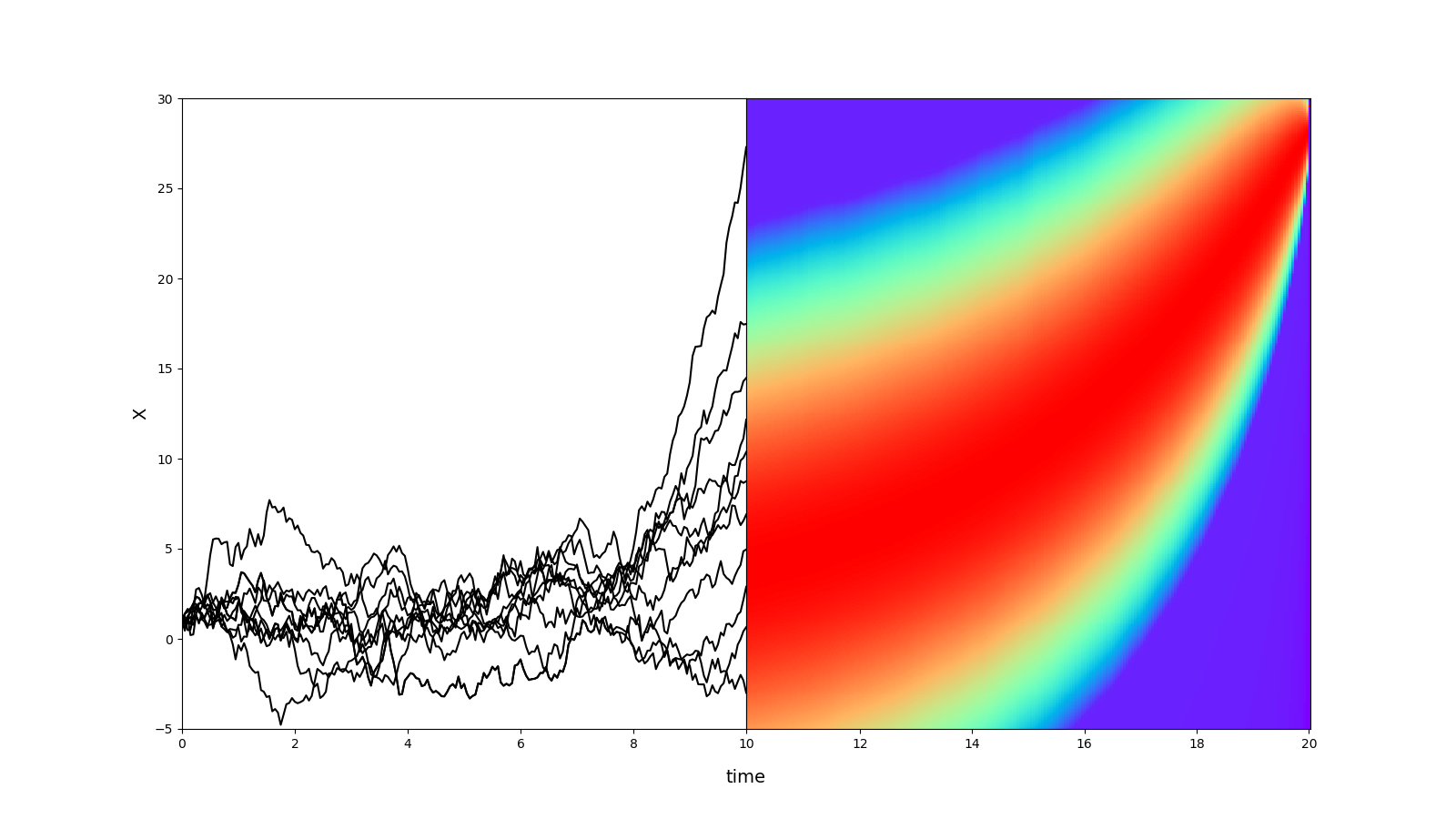
Figure 2: Illustration of the resampling step at time $t=10$ in cSMC. The left side shows several forward paths $x_{0:t}^{(i)}$ to be resampled, and the right side shows the heatmap of $p({\cal I}_{t+1:t_{+}}\,|\,x_{0:t})$.

In the proposed cSMC algorithm, we point out that the sample set $\{(x_{t}^{(i)},w_{t}^{(i)})\}_{i=1,\cdots,n}$ obtained at each time $t<T$ is properly weighted with respect to $\mathbb{P}^{0}_{t}$, not the desired $\mathbb{P}_{t}^{*}$. However, $\big{\{}(x_{t}^{(i)},w_{t}^{(i)}p(\mathcal{I}_{t+1:t+}|x_{0:t}^{(i)})\big{\}}_{i=1,\cdots,n}$ is properly weighted with respect to $\mathbb{P}_{t}^{*}$. Unfortunately it is not operational since one would need to be able to calculate $p(\mathcal{I}_{t+1:t+}|x_{0:t})$ precisely.

As pointed out by Liu and Chen (1998), conducting resampling at every time $t$ is not necessary. It increases computational costs and introduces additional variation to the current sample set. Liu and Chen (1998) proposed to carry out the resampling step at a pre-determined schedule, say, performing resampling at $t=k,2k,\cdots$, or when the effective sample size is below a certain threshold. The effective sample size (ESS) at time $t$ is defined as

$$\text{ESS}_{t}=\frac{n}{1+\widehat{\text{var}}(\beta_{t})/\overline{\beta}_{t}^{2}}=\frac{\left(\sum_{i=1}^{n}\beta_{t}^{(i)}\right)^{2}}{\sum_{i=1}^{n}(\beta_{t}^{(i)})^{2}},$$ (4)

where $\overline{\beta}_{t}=\frac{1}{n}\sum_{i=1}^{n}\beta_{t}^{(i)}$ and $\widehat{\text{var}}(\beta_{t})=\frac{1}{n}\sum_{i=1}^{n}\big{(}\beta_{t}^{(i)}-\overline{\beta}_{t}\big{)}^{2}$. Here the ESS_t measures the variation of the priority scores $\{\beta_{t}^{(i)}\}_{i=1,\cdots,n}$.

3 Special Cases

In this section, we discuss several special cases of constrained sampling problems. All these problems can be effectively solved under the cSMC Algorithm in Figure 1, by specifying $\mathcal{I}_{t}$ and the ”ideal” priority score $\beta_{t}^{(i)}$ in (3). We will discuss how to approximate $\beta_{t}^{(i)}$ in Section 4.

3.1 Frequent Constrained Problems – the State Space Model

Consider a type of frequent constraint problems where $x_{0:T}=(x_{0},x_{1},\cdots,x_{T})$ is a stochastic process governed by a forward propagation equation $p(x_{t}|x_{t-1})$ and at each time $t$, we observe $y_{t}$ which is related to $x_{t}$ with uncertainty. Suppose that the distribution of $y_{t}$ is entirely determined by $x_{t}$ through a conditional distribution $p(y_{t}\,|\,x_{t})$. Such a system is often called a state space model. The observed sequence $y_{0:T}=(y_{0},\cdots,y_{T})$ can be viewed as a set of frequent constraints.

This problem can be solved by sampling $x_{0:T}$ first using the forward propagation equation, and then re-weighting the paths by $p(y_{0:T}|x_{0:T})=\prod_{t=0}^{T}p(y_{t}\,|\,x_{t})$, though it is not efficient. The standard SISR method recursively utilizes the information $\mathcal{I}_{t}=\{y_{t}\}$ during the propagation. It has been shown to be extremely useful and efficient if implemented properly. A variety of SISR implementations are actually special cases of cSMC.

Similar to the algorithm in Figure 1, the Bayesian bootstrap filter proposed in Gordon et al. (1993) uses $q(x_{t}|x_{0:t-1})=p(x_{t}|x_{t-1})$ for propagation and the weights are updated by $w_{t}^{(i)}=w_{t-1}^{(i)}p(y_{t}|x_{t}^{(i)})$. Kong et al. (1994) and Liu and Chen (1998) adopted a proposal distribution $q(x_{t}|x_{0:t-1})$ $\propto p(x_{t}|x_{t-1})p(y_{t}\,|\,x_{t})$, which incorporates the current information ${\cal I}_{t}=\{y_{t}\}$ for sampling. When the current observation contains strong information about $x_{t}$, Lin et al. (2005) proposed to draw state samples from $q(x_{t}|x_{0:t-1})\propto p(y_{t}\,|\,x_{t})$. All above methods use $\beta_{t}^{(i)}=w_{t}^{(i)}$ for resampling, which is the case that $t_{+}$ always equals $t$ in cSMC. The auxiliary particle filter (APF) proposed in Pitt and Shephard (1999) uses a different approach. The APF conducts resampling with the priority score $\beta_{t}^{(i)}=w_{t}^{(i)}p(y_{t+1}\,|\,x_{t}^{(i)})$, which is the case $t_{+}=t+1$ in cSMC. They showed that it is often more efficient to incorporate the future information $\mathcal{I}_{t+1}=\{y_{t+1}\}$ for resampling. Chen et al. (2000) and Lin et al. (2013) proposed the delayed sampling method, in which the priority score $\beta_{t}^{(i)}=w_{t}^{(i)}p(y_{t+1},\dots,y_{t+\Delta}\,|\,x_{t}^{(i)})$ uses future information up to a fixed delay of $\Delta$ time units. In this case, $t_{+}=t+\Delta$.

3.2 Strong Constrained Problems

A constraint set $\mathcal{I}_{0:T}$ is said to be extremely strong if the likelihood function $p(\mathcal{I}_{0:T}|x_{0:T})=0$ almost surely under the system dynamics $p(x_{0:T})$. That is, the constraints will never be satisfied if we use the system dynamics to generate samples.

One example with extremely strong constraints is the diffusion bridge sampling problem considered in Pedersen (1995); Durham and Gallant (2002) and Lin et al. (2010). Suppose that a continuous-time process $\{X_{\lambda}\}_{0\leq\lambda\leq\Lambda}$ is governed by a diffusion stochastic differential equation

$$dX_{\lambda}=\mu(X_{\lambda},{\lambda})d{\lambda}+\sigma(X_{\lambda},{\lambda})dW_{\lambda},$$ (5)

where $\mu(X_{\lambda},\lambda)$ and $\sigma(X_{\lambda},\lambda)$ are the corresponding drift and diffusion coefficients, and $\{W_{\lambda}\}_{0\leq\lambda\leq\Lambda}$ is a standard Brownian motion. We want to generate bridge samples that connect two fixed end points $X_{0}=a$ and $X_{\Lambda}=b$.

Let $0=\tau_{0}<\tau_{1}<\cdots<\tau_{T-1}<\tau_{T}=\Lambda$ be a sequence of equally-spaced intermediate points and let $\delta=\tau_{t}-\tau_{t-1}$. By the Euler-Maruyama method, system (5) can be approximated by

$$X_{\tau_{t}}=X_{\tau_{t-1}}+\mu(X_{\tau_{t-1}},\tau_{t-1})\delta+\sigma(X_{\tau_{t-1}},\tau_{t-1})(W_{\tau_{t}}-W_{\tau_{t-1}})+o_{p}\big{(}\sqrt{\delta}\big{)},$$

where $o_{p}\big{(}\sqrt{\delta}\big{)}$ denotes the error term in discretization. High accuracy can be achieved by increasing the number of intermediate points at the cost of additional computational burden. In most applications, choosing the appropriate number of intermediate points is a compromise between the discretization error and the computational efficiency.

The continuous-time stochastic process $\{X_{\lambda}\}_{0\leq\lambda\leq\Lambda}$ now is approximated by the discrete-time process $x_{0:T}$, where $x_{t}=X_{\tau_{t}}$ and $p(x_{t}\,|\,x_{t-1})\sim N\big{(}x_{t-1}+\mu(x_{t-1},\tau_{t-1})\delta,\sigma^{2}(x_{t-1},\tau_{t-1})\delta\big{)}$. Thus, it becomes a sampling problem with the highly constrained target distribution $p(x_{0:T}\,|\,x_{0}=a,x_{T}=b)$. Pedersen (1995) used $q(x_{t}\mid x_{0:t-1})=p(x_{t}\,|\,x_{t-1})$ to generate sample paths, and all paths are forced to connect to the fixed end point in the last step. Durham and Gallant (2002) proposed a method based on SMC with linear interpolation as the proposal distribution. Lin et al. (2010) developed a method under the cSMC framework with $t_{+}=T$ for all $t$. In their method, a backward pilot approach is used to approximate the term $p(I_{t+1:t_{+}}\,|\,x_{t})=p(x_{T}=b\,|\,x_{t})$ in (3). Lin et al. (2010) showed that using a priority score based on the end point constraint can effectively improve the sampling efficiency.

3.3 Systems with Intermediate Constraints

The cSMC algorithm can also be applied to the cases with sparse intermediate constraints, which are infrequent but relatively strong. Suppose the stochastic process $x_{0:T}$ is Markovian and is governed by $p(x_{t+1}\,|\,x_{t})$, and noisy observations come in periodically. For simplicity, we assume that $T=KM$, and $y_{k}$ is a noisy measurement of $x_{kM}$ for $k=1,\cdots,K$. Here we propose a sampling procedure for $x_{0:T}$ given the information set $y_{1:K}$ under the general cSMC framework.

The intermediate observations split the whole path into $K$ segments as shown in Figure 3. In the first segment, the path $(x_{0},x_{1},\cdots,x_{M},y_{1})$ can be viewed as a new system, in which $y_{1}$ is part of the stochastic process and the observation equation $p(y_{1}\,|\,x_{M})$ for $y_{1}$ works as the state equation of $y_{1}$ conditioned on $x_{M}$. Under such a setting, $y_{1}$ is now the fixed-point constraint at $t=M+1$. We can first draw initial samples from $q(x_{0})=p(x_{0})$, then propagate to $x_{M}$ based on a procedure similar to sampling diffusion bridges in Section 3.2. In the end, we can obtain samples from distribution $p(x_{0:M}\,|\,y_{1})$. These samples of $x_{0:M}$ can be used as the initial samples for the next segment, repeated until reaching the last segment, at which time the weighted sample set $\big{\{}(x_{0:T}^{(i)},w_{T}^{(i)})\big{\}}_{i=1,\dots,n}$ follows the desired distribution $p(x_{0:T}\,|\,y_{1},\dots,y_{K})$.

Figure 3: Segmentation of a stochastic process with intermediate observations.

3.4 Systems with Multilevel Constraints

The cSMC strategy can also be used to solve problems with multiple levels of constraints, including those with a hierarchical structure, such as one level of weak but frequent constraints and another level of strong but infrequent constraints. A special case is a standard state space model with two fixed endpoint constraints. Specifically, suppose a state space model is governed by the state dynamics $p(x_{t}\,|\,x_{t-1})$ and the observation equation $p(y_{t}\,|\,x_{t})$. In addition, two fixed endpoint constraints are imposed on $x_{0:T}$ with $x_{0}=a$ and $x_{T}=b$. Again, we want to draw samples from the conditional distribution $p(x_{0:T}\,|\,x_{0}=a,y_{1:T-1},x_{T}=b)$.

The routine observations $y_{1},\cdots,y_{T-1}$ can be viewed as a layer of weak constraints and the fixed point constraints are viewed as a layer of strong constraints. To utilize the cSMC method, we can suppress the weak constraints layer and define $t_{+}=T$ for $t>0$. That is, the priority score is chosen as $\beta_{t}^{(i)}=w_{t}^{(i)}\,p(y_{t+1:T-1},\,x_{T}=b\,|\,x_{t}^{(i)})$ in the resampling step.

4 Approximation of the Priority Score in cSMC

We consider the evaluation of the term $p(\mathcal{I}_{t+1:t_{+}}\,|\,x_{0:t})$ in the priority score (3). Let the time stamps of the strong constraints be $T_{0}<T_{1}<\cdots<T_{K}$. For the ease of presentation, we always assume that $T_{0}=0$ in the following. Here we omit the trivial case that $t_{+}=t$, in which $p(\mathcal{I}_{t+1:t_{+}}\,|\,x_{0:t})=1$, and focus on the case that $T_{k-1}<t<T_{k}$ for some $k$. Then

$$p(\mathcal{I}_{t+1:t+}|x_{0:t})=p(\mathcal{I}_{t+1:T_{k}}|x_{0:t})=\int\cdots\int\prod_{s=t+1}^{T_{K}}p(x_{s}\,|\,x_{0:s-1})p(\mathcal{I}_{s}\,|\,x_{0:s})dx_{t+1}\cdots dx_{T_{K}}.$$ (6)

The integrand is often well-defined by the model, but in most cases the integration does not have a closed-form solution. In this section, we present several different methods to approximate $p(\mathcal{I}_{t+1:t_{+}}|x_{0:t})$.

4.1 Optimized Parametric Priority Scores

Based on some prior information, one may assume a parametric form for $p(\mathcal{I}_{t+1:t+}|x_{0:t})$. Zhang et al. (2007) and Lin et al. (2008) used the cSMC approach with $t_{+}=T$ to generate protein conformation samples satisfying certain residue distance constraints. The parametric functions they used to approximate $p(\mathcal{I}_{t+1:t+}|x_{0:t})$ are based on residue distance information of the partial chain $x_{0:t}$.

The particle efficient importance sampling (PEIS) method of Scharth and Kohn (2016) uses locally optimized parametric priority scores. Here we present PEIS under cSMC framework and notations. When the stochastic dynamic system is Markovian, that is,

$$p(x_{t}\,|\,x_{0:t-1})=p(x_{t}\,|\,x_{t-1})\quad\text{and}\quad p(\mathcal{I}_{t}\,|\,x_{0:t})=p(\mathcal{I}_{t}\,|\,x_{t}),$$

for all $t$, PEIS approximates $p(\mathcal{I}_{t+1:T}|x_{0:t})$ and finds a series of proposal distributions $q(x_{t}\,|\,x_{t-1})$ close to $p(x_{t}\,|\,x_{t-1},\mathcal{I}_{t:T})$ for $t=0,1,\cdots,T$. Specifically, PEIS sets

$$q(x_{t}\,|\,x_{t-1};\theta_{t})=\psi_{t}(x_{t},x_{t-1};\theta_{t})/\chi_{t}(x_{t-1};\theta_{t}),$$

where $\psi_{t}(x_{t},x_{t-1};\theta_{t})$ is in a parametric family with parameter $\theta_{t}$, and $\chi_{t}(x_{t-1};\theta_{t})=\int\psi_{t}(x_{t},x_{t-1};\theta_{t})\,dx_{t}$ is the normalizing term. Then the importance weight at time $T$ becomes

$$w_{T}(x_{0:T}) = \frac{p(x_{0:T}\,|\,\mathcal{I}_{0:T})}{q(x_{0};\theta_{0})\prod_{t=1}^{T}q(x_{t}\,|\,x_{t-1};\theta_{t})}$$ (7)

$$\propto \frac{p(x_{0})p(\mathcal{I}_{0}\,|\,x_{0})\prod_{t=1}^{T}p(x_{t}\,|\,x_{t-1})p(\mathcal{I}_{t}\,|\,x_{t})}{q(x_{0};\theta_{0})\prod_{t=1}^{T}q(x_{t}\,|\,x_{t-1};\theta_{t})}$$

$$\propto \frac{p(x_{0})\chi_{1}(x_{0};\theta_{1})}{\psi_{0}(x_{0};\theta_{0})}\left[\prod_{t=1}^{T-1}\frac{p(x_{t}\,|\,x_{t-1})p(\mathcal{I}_{t}\,|\,x_{t})\chi_{t+1}(x_{t};\theta_{t+1})}{\psi_{t}(x_{t},x_{t-1};\theta_{t})}\right]\frac{p(x_{T}\,|\,x_{T-1})p(\mathcal{I}_{T}\,|\,x_{T})}{\psi_{T}(x_{T},x_{T-1};\theta_{T})},$$

where the initial $\psi_{0}(x_{0};\theta_{0})$ is also restricted in a parametric family. To ensure that the difference between the target distribution $p(x_{0:T}\,|\,\mathcal{I}_{0:T})$ and the proposal distribution $q(x_{0};\theta_{0})\prod_{t=1}^{T}q(x_{t}\,|\,x_{t-1};\theta_{t})$ is small, Equation (7) suggests to minimize the variation of each term in the product. Hence, we start with an optimal $\theta_{T}$ that minimizes the variation of the ratio

$$\frac{p(x_{T}\,|\,x_{T-1})p(\mathcal{I}_{T}\,|\,x_{T})}{\psi_{T}(x_{T},x_{T-1};\theta_{T})}.$$

Then going backward recursively, for $t=T-1,\dots,1$, we find $\theta_{t}$ that minimizes the variation of

$$\frac{p(x_{t}\,|\,x_{t-1})p(\mathcal{I}_{t}\,|\,x_{t})\chi_{t+1}(x_{t};\theta_{t+1})}{\psi_{t}(x_{t},x_{t-1};\theta_{t})}.$$

The PEIS method can be easily adapted to our settings to approximate $p(\mathcal{I}_{t+1:t+}|x_{0:t})$. The algorithmic steps to find the “optimal” parameters are presented in Figure 4. We repeat the optimization procedure for each time interval from $T_{k-1}+1$ to $T_{k}$ to find the “optimal” parameter $\theta_{t}$ for every $T_{k-1}<t\leq T_{k}$. Then the normalizing term $\chi_{t+1}(x_{t};\theta_{t+1})$ can be used as an approximation of $p(\mathcal{I}_{t+1:t+}|x_{0:t})$. We note that the performance of this method greatly depends on the choice of the parametric family for $\psi_{t}(x_{t},x_{t-1};\theta_{t})$.

Figure 4: PEIS Parameter Optimization Algorithm under cSMC Framework • For $k=1,\cdots,K$: – Initialize the parameters $\theta_{t}^{[0]}$ for $t=T_{k-1}+1,\cdots,T_{k}$. – Update the parameters iteratively as follows. * Generate samples $x_{T_{k-1}:T_{k}}^{(j)}$, $j=1,\cdots,m$, from the proposal distribution $\displaystyle q(x_{T_{k-1}})\prod_{t=T_{k-1}+1}^{T_{k}}q(x_{t}\,|\,x_{t-1};\theta_{t}^{[l-1]}),$ where $q(x_{T_{k-1}})$ is a distribution close to $p(\mathcal{I}_{T_{k-1}}\,|\,x_{T_{k-1}})$. * Calculate the weights $\displaystyle w_{T_{k}}^{(j)}=\frac{p(\mathcal{I}_{T_{k-1}}\,|\,x_{T_{k-1}}^{(j)})}{q(x_{T_{k-1}}^{(j)})}\prod_{t=T_{k-1}+1}^{T_{k}}\frac{p(x_{t}^{(j)}\,|\,x_{t-1}^{(j)})p(\mathcal{I}_{t}\,|\,x_{t}^{(j)})}{q(x_{t}^{(j)}\,|\,x_{t-1}^{(j)};\theta_{t}^{[l-1]})}$ * For $t=T_{k},T_{k}-1,\cdots,T_{k-1}+1$, solve the minimization problem $\displaystyle(\theta_{t}^{[l]},b_{t}^{[l]})=\arg\min_{\theta,\gamma}\sum_{j=1}^{m}w_{T_{k}}^{(j)}\Big{\{}\log\big{[}p(x_{t}^{(j)}\,|\,x_{t-1}^{(j)})p(\mathcal{I}_{t}\,|\,x_{t}^{(j)})\chi_{t+1}(x_{t}^{(j)};\theta_{t+1}^{[l]})\big{]}$ $\displaystyle\hskip 213.39566pt-\gamma-\log\big{[}\psi_{t}(x_{t}^{(j)},x_{t-1}^{(j)};\theta)\big{]}\Big{\}}^{2},$ where $\chi_{t+1}(x_{t};\theta_{t+1})$ is set to a constant when $t=T_{K}$. * Stop the iteration until the parameters converge. Let $\theta_{t}^{*}$, $t=T_{k-1}+1,T_{k}-1,\cdots,T_{k}$, denote the converged parameters. • Return the estimated functions $\Big{\{}\widehat{p}(\mathcal{I}_{t+1:t_{+}}\,|\,x_{0:t})=\chi_{t+1}(x_{t};\theta_{t+1}^{*})\Big{\}}_{t=T_{k-1}+1,\cdots,T_{k}-1;k=1,\cdots,K}$ to compute the priority scores in Figure 1.

4.2 Priority Scores Based on Forward Pilots

When it is not easy to choose an appropriate parametric family for $p(x_{t},\mathcal{I}_{t}\,|\,x_{0:t-1})$, we may consider to send out pilot samples to estimate the integration (6) by nonparametric methods. The pilot sample idea has been proposed by Wang et al. (2002) and Zhang and Liu (2002), and is used for delayed estimation in SMC (Lin et al., 2013). Specifically, suppose at time $t$ we have the samples $\{(x_{0:t}^{(i)},w_{t}^{(i)})\}_{i=1,\cdots,n}$ properly weighted with respect to $\mathbb{P}^{0}_{t}$. For each sample $x_{0:t}^{(i)}$, the pilot samples $\widetilde{x}_{t+1:t_{+}}^{(i,j)}=(\widetilde{x}_{t+1}^{(i,j)},\cdots,\widetilde{x}_{t_{+}}^{(i,j)})$, $j=1,\cdots,J$, are generated from a proposal distribution $\prod_{s=t+1}^{t_{+}}g(x_{s}\,|\,x_{0:t}^{(i)},x_{t+1:s-1})$ and are weighted by $U_{t}^{(i,j)}=\prod_{s=t+1}^{t_{+}}u_{s}^{(i,j)}$ with

$$u_{s}^{(i,j)}=\frac{p(\widetilde{x}_{s}^{(i,j)}\,|\,x_{0:t}^{(i)},\widetilde{x}_{t+1:s-1}^{(i,j)})p(\mathcal{I}_{s}\,|\,x_{0:t}^{(i)},\widetilde{x}_{t+1:s}^{(i,j)})}{g(\widetilde{x}_{s}^{(i,j)}\,|\,x_{0:t}^{(i)},\widetilde{x}_{t+1:s-1}^{(i,j)})}.$$

It is easy to see that $E(U_{t}^{(i,j)}\,|\,x_{0:t}^{(i)})=p(\mathcal{I}_{t+1:t+}|x_{0:t}^{(i)})$. Hence we can use $\widehat{p}(\mathcal{I}_{t+1:t_{+}}\,|\,x_{0:t}^{(i)})=\frac{1}{J}\sum_{j=1}^{J}U_{t}^{(i,j)}$ to approximate $p(\mathcal{I}_{t+1:t+}|x_{0:t}^{(i)})$. However, the computational cost of this method is relatively high since it requires the generation of pilot samples for every path $x_{0:t}^{(i)}$ at every time $t$.

Suppose there exists a low dimensional statistic $S(x_{0:t})$ that summarizes $x_{0:t}$ such that

$$p(x_{t}\,|\,x_{0:t-1})=p\big{(}x_{t}\,|\,S(x_{0:t-1})\big{)}\quad\text{and}\quad p(\mathcal{I}_{t}\,|\,x_{0:t})=p\big{(}\mathcal{I}_{t}\,|\,S(x_{0:t})\big{)}$$ (8)

for all $t$, and suppose we have a function $\phi(\cdot)$ such that $S(x_{0:t})=\phi\big{(}S(x_{0:t-1}),x_{t}\big{)}$. Then, $p(\mathcal{I}_{t+1:t+}\,|\,x_{0:t})$ $=p(\mathcal{I}_{t+1:t+}\,|\,S(x_{0:t}))$ is a function of $S(x_{0:t})$. The idea is to use a smoothing technique on the low dimensional $S(x_{0:t})$ to reduce the computational cost. The algorithm is presented in Figure 5. Note that for $U_{t}^{(j)}=\prod_{s=t+1}^{T_{k}}\widetilde{u}_{s}^{(j)}$ defined in Figure 5, we have

$$E(U_{t}^{(j)}\,|\,S_{t}^{(j)}=S)=p(\mathcal{I}_{t+1:t+}|S(x_{0:t})=S).$$

Therefore, we can use $\big{\{}(U_{t}^{(j)},S_{t}^{(j)})\big{\}}_{j=1,\cdots,m}$ to estimate $p\big{(}\mathcal{I}_{t+1:t+}|S(x_{0:t})\big{)}$ by the nonparametric histogram function (9) in Figure 5. We choose not to use the kernel smoothing method here in order to control the computational cost, because $\widehat{p}(\mathcal{I}_{t+1:t_{+}}|S(x_{0:t}))$ needs to be evaluated for all $x_{0:t}^{(j)},j=1,\dots,n$ and at each time $t$. Compared with the pilot sampling method proposed in Wang et al. (2002), this algorithm only need to be conducted once to obtain $\widehat{p}\big{(}\mathcal{I}_{t+1:t_{+}}\,|\,S(x_{0:t})\big{)}$ for all $t$.

The accuracy of $\widehat{p}\big{(}\mathcal{I}_{t+1:t_{+}}\,|\,S(x_{0:t})\big{)}$ depends on the choice of the proposal distribution $g(x_{s}\,|\,x_{0:t}^{(i)},$ $x_{t+1:s-1})$ to generate the pilots. Since $\mathcal{I}_{T_{k}}$ is a strong constraint, when generating pilot samples from $T_{k-1}+1$ to $T_{k}$, we need to incorporate the information from $\mathcal{I}_{T_{k}}$ in the proposal distribution $g(\cdot)$, so that the pilot samples will have a reasonable large probability to satisfy the constraint $\mathcal{I}_{T_{k}}$.

Figure 5: Forward Pilot Smoothing Algorithm • For $k=1,\cdots,K$: – Initialization: For $j=1,\cdots,m$, draw samples $S_{T_{k-1}}^{(j)}$ from a proposal distribution $g(S)$ that covers the support of $S(x_{0:T_{k-1}})$. – For $t=T_{k-1}+1,\cdots,T_{k}$, draw pilot samples forwardly as follows. * Generate samples $\widetilde{x}_{t}^{(j)}$ from a proposal distribution $g(\widetilde{x}_{t}\,|\,S_{t-1}^{(j)})$, and calculate $S_{t}^{(j)}=\phi(S_{t-1}^{(j)},\widetilde{x}_{t}^{(j)})$ for $j=1,\cdots,m$. * Calculate the incremental weights $\displaystyle\widetilde{u}_{t}^{(j)}=\frac{p(\widetilde{x}_{t}^{(j)}\,|\,S(\widetilde{x}_{0:t-1}^{(j)})=S_{t-1}^{(j)})p(\mathcal{I}_{t}\,|\,S(\widetilde{x}_{0:t}^{(j)})=S_{t}^{(j)})}{g(\widetilde{x}_{t}^{(j)}\,|\,S_{t-1}^{(j)})},\quad j=1,\cdots,m.$ – For $t=T_{k-1}+1,\cdots,T_{k}-1$: * Compute $U_{t}^{(j)}=\prod_{s=t+1}^{T_{k}}\widetilde{u}_{s}^{(j)}$ for $j=1,\cdots,m$. * Let $\mathcal{S}_{1}\cup\cdots\cup\mathcal{S}_{D}$ be a partition of the support of $S(x_{0:t})$. Estimate $p(\mathcal{I}_{t+1:t_{+}}\,|\,x_{0:t})=p(\mathcal{I}_{t+1:t_{+}}|S(x_{0:t}))$ by $\displaystyle f_{t}(S(x_{0:t}))=\sum_{d=1}^{D}\xi_{t,d}\mathbb{I}\big{(}S(x_{0:t})\in\mathcal{S}_{d}\big{)}$ (9) with $\displaystyle\xi_{t,k}=\frac{\sum_{j=1}^{m}U_{t}^{(j)}\mathbb{I}\big{(}S_{t}^{(j)}\in\mathcal{S}_{d}\big{)}}{\sum_{j=1}^{m}\mathbb{I}\big{(}S_{t}^{(j)}\in\mathcal{S}_{d}\big{)}}.$ where $\mathbb{I}(\cdot)$ is the indicator function. • Return the estimated functions $\Big{\{}\widehat{p}(\mathcal{I}_{t+1:t_{+}}\,|\,x_{0:t})=f_{t}(S(x_{0:t}))\Big{\}}_{t=T_{k-1}+1,\cdots,T_{k}-1;k=1,\cdots,K}$ to compute the priority scores in Figure 1.

4.3 Priority Scores Based on Backward Pilots

When the stochastic dynamic system is Markovian, we can extend the backward pilot sampling method proposed in Lin et al. (2010) to the cSMC settings. In this sampling method, the pilot samples are generated in the opposite time direction, starting from the highly constrained time point $T_{k}$ and propagating backward. The algorithm is presented in Figure 6.

In this algorithm, the weight for the backward pilot $\widetilde{x}_{t:t_{+}}$ is

$$\widetilde{w}_{t}=\frac{p(\widetilde{x}_{t+1:t_{+}},\mathcal{I}_{t+1:t_{+}}\,|\,\widetilde{x}_{t})}{r(\widetilde{x}_{t:t_{+}})},$$

where $r(\widetilde{x}_{t:t_{+}})$ is the proposal distribution to generate the backward pilots. Taking expectation conditional on $\widetilde{x}_{t}$, we have

$$E(\widetilde{w}_{t}\,|\,\widetilde{x}_{t}) = \int\cdots\int\frac{p(\widetilde{x}_{t+1:t_{+}},\mathcal{I}_{t+1:t_{+}}\,|\,\widetilde{x}_{t})}{r(\widetilde{x}_{t},\widetilde{x}_{t+1:t_{+}})}\,r(\widetilde{x}_{t+1:t_{+}}\,|\,\widetilde{x}_{t})d\widetilde{x}_{t+1:t_{+}}$$

$$= p(\mathcal{I}_{t+1:t+}|\widetilde{x}_{t})/r(\widetilde{x}_{t}^{(j)}),$$

where $r(\widetilde{x}_{t+1:t_{+}}\,|\,\widetilde{x}_{t})$ and $r(\widetilde{x}_{t})$ are the conditional distribution and the marginal distribution induced from $r(\widetilde{x}_{t:t_{+}})$, respectively. Therefore,

$$p(\mathcal{I}_{t+1:t+}|\widetilde{x}_{t})=r(\widetilde{x}_{t})E(\widetilde{w}_{t}\,|\,\widetilde{x}_{t}).$$

Again, we can use the pilot samples $\big{\{}(\widetilde{x}_{t}^{(j)},\widetilde{w}_{t}^{(j)})\big{\}}_{j=1,\cdots,m}$ to estimate $r(\widetilde{x}_{t})$ and $E(\widetilde{w}_{t}\,|\,\widetilde{x}_{t})$ by nonparametric smoothing. A histogram estimator is

$$\widehat{p}(\mathcal{I}_{t+1:t+}|x_{t}) = \widehat{r}(x_{t})\widehat{E}(\widetilde{w}_{t}\,|\,x_{t})$$

$$= \sum_{d=1}^{D}\frac{\sum_{j=1}^{m}\mathbb{I}\big{(}\widetilde{x}_{t}^{(j)}\in\mathcal{X}_{d}\big{)}}{m|\mathcal{X}_{d}|}\mathbb{I}\big{(}x_{t}\in\mathcal{X}_{d}\big{)}\cdot\sum_{d=1}^{D}\frac{\sum_{j=1}^{m}\widetilde{w}_{t}^{(j)}\mathbb{I}\big{(}\widetilde{x}_{t}^{(j)}\in\mathcal{X}_{d}\big{)}}{\sum_{j=1}^{m}\mathbb{I}\big{(}\widetilde{x}_{t}^{(j)}\in\mathcal{X}_{d}\big{)}}\,\mathbb{I}\big{(}x_{t}\in\mathcal{X}_{d}\big{)}$$

$$= \sum_{d=1}^{D}\frac{\sum_{j=1}^{m}\widetilde{w}_{t}^{(j)}\mathbb{I}\big{(}\widetilde{x}_{t}^{(j)}\in\mathcal{X}_{d}\big{)}}{m|\mathcal{X}_{d}|}\,\mathbb{I}\big{(}x_{t}\in\mathcal{X}_{d}\big{)},$$

where $\mathcal{X}_{1}\cup\mathcal{X}_{2}\cup\cdots\cup\mathcal{X}_{D}$ is a partition of the support of $x_{t}$ and $|\mathcal{X}_{d}|$ denotes the volume of $\mathcal{X}_{d}$.

Compared with the forward pilot method, the backward pilots here are generated backward, starting from the constrained time point $T_{k}$. The strong constraint $\mathcal{I}_{T_{K}}$ is automatically incorporated in the proposal distribution to generate $\widetilde{x}_{T_{k}}$ at the beginning. Hence it is often expected to have a more accurate approximation estimation of $p(\mathcal{I}_{t+1:t+}|x_{t})$. However, it requires the system to be Markovian to apply this method.

Figure 6: Backward Pilot Smoothing Algorithm • For $k=1,\cdots,K$: – Initialization: For $j=1,\cdots,m$, draw samples $\widetilde{x}_{T_{k}}^{(j)}$ from a proposal distribution $r(x_{T_{k}})$ and set $\widetilde{w}_{T_{k}}^{(j)}=1/r(\widetilde{x}_{T_{k}}^{(j)})$. – For $t=T_{k}-1,\cdots,T_{k-1}+1$, draw pilot samples backward as follows. * Generate samples $\widetilde{x}_{t}^{(j)}$, $j=1,\cdots,m$, from a proposal distribution $r(\widetilde{x}_{t}\,|\,\widetilde{x}_{t+1}^{(j)})$. * Update weights by $\displaystyle\widetilde{w}_{t}^{(j)}=\widetilde{w}_{t+1}^{(j)}\frac{p(\widetilde{x}_{t+1}^{(j)}\,|\,\widetilde{x}_{t}^{(j)})p(\mathcal{I}_{t+1}\,|\,\widetilde{x}_{t+1}^{(j)})}{r(\widetilde{x}_{t}^{(j)}\,|\,\widetilde{x}_{t+1}^{(j)})},\quad j=1,\cdots,m.$ * Let $\mathcal{X}_{1}\cup\cdots\cup\mathcal{X}_{D}$ be a partition of the support of $x_{t}$. Estimate $p(\mathcal{I}_{t+1:t_{+}}\,|\,x_{0:t})=p(\mathcal{I}_{t+1:t_{+}}\,|\,x_{t})$ by $\displaystyle f_{t}(x_{t})=\sum_{d=1}^{D}\eta_{t,d}\mathbb{I}\big{(}x_{t}\in\mathcal{X}_{d}\big{)},$ where $\displaystyle\eta_{t,d}=\frac{1}{m|\mathcal{X}_{d}|}\sum_{j=1}^{m}\widetilde{w}_{t}^{(j)}\mathbb{I}(\widetilde{x}_{t}^{(j)}\in\mathcal{X}_{d}),$ and $|\mathcal{X}_{d}|$ denotes the volume of the subset $\mathcal{X}_{d}$. • Return the estimated functions $\Big{\{}\widehat{p}(\mathcal{I}_{t+1:t_{+}}\,|\,x_{0:t})=f_{t}(x_{t})\Big{\}}_{t=T_{k-1}+1,\cdots,T_{k}-1;k=1,\cdots,K}$ to compute the priority scores in Figure 1.

5 Examples

5.1 Computing Long-Run Marginal Expected Shortfall

It is important to measure the systemic risk of a firm for risk control. Acharya et al. (2012) proposed to use the long-run marginal expected shortfall (LRMES) as a systemic risk index, which is defined as the expected capital shortfall of a firm during a financial crisis. Particularly, if the market index falls by 40% in the next six months (126 trading days), it is viewed as a financial crisis. Let $x_{m,t}$ and $x_{f,t}$ be the daily logarithmic prices of the market and the firm at time $t$, respectively. The LRMES of the firm is defined as

$$\text{LRMES}=E\big{(}1-e^{x_{f,T}-x_{f,0}}\,|\,e^{x_{m,T}-x_{m,0}}<0.6\big{)}$$

with $T=126$.

Following Brownlees and Engle (2012) and Duan and Zhang (2016), we assume that $\{(x_{m,t},x_{f,t})\}_{t=0,1,\cdots,T}$ follows a bivariate GJR-GARCH model. Without loss of generality, let $x_{m,0}=x_{f,0}=0$ and

$$x_{m,t} = x_{m,t-1}+\sigma_{m,t}\epsilon_{m,t},$$ (10)

$$\sigma_{m,t}^{2} = \omega_{m}+\big{[}\alpha_{m}+\gamma_{m}\mathbb{I}(\epsilon_{m,t-1}<0)\big{]}(\sigma_{m,t-1}\epsilon_{m,t-1})^{2}+\beta_{m}\sigma_{m,t-1}^{2},$$

$$x_{f,t} = x_{f,t-1}+\sigma_{f,t}\epsilon_{f,t}=x_{f,t-1}+\sigma_{f,t}\left(\rho_{f,t}\epsilon_{m,t}+\sqrt{1-\rho_{f,t}^{2}}\,\xi_{f,t}\right),$$

$$\sigma_{f,t}^{2} = \omega_{f}+\big{[}\alpha_{f}+\gamma_{f}\mathbb{I}(\epsilon_{f,t-1}<0)\big{]}(\sigma_{f,t-1}\epsilon_{f,t-1})^{2}+\beta_{f}\sigma_{f,t-1}^{2},$$

where $\epsilon_{m,t}\sim N(0,1)$ and $\xi_{f,t}\sim N(0,1)$; $\{\epsilon_{m,t}\}_{t=1,\cdots,T}$ and $\{\xi_{f,t}\}_{t=1,\cdots,T}$ are independent with each other and independent over time. The time-varying correlation coefficients $\{\rho_{f,t}\}_{t=1,\cdots,T}$ are modeled by the dynamic conditional correlation (DCC) approach. To be specified, let $Q_{f,1},\cdots,Q_{f,T}$ be a sequence of $2\times 2$ covariance matrices satisfying

$$Q_{f,t} = (1-\alpha_{C}-\beta_{C})\overline{Q}_{f}+\alpha_{C}\left(\begin{array}[]{c}\sigma_{m(t-1)}\epsilon_{m(t-1)}\\ \sigma_{f(t-1)}\epsilon_{f(t-1)}\\ \end{array}\right)\left(\begin{array}[]{c}\sigma_{m(t-1)}\epsilon_{m(t-1)}\\ \sigma_{f(t-1)}\epsilon_{f(t-1)}\\ \end{array}\right)^{\prime}+\beta_{C}Q_{f(t-1)},$$ (15)

and $\rho_{f,t}$ is defined as the correlation coefficient induced by $Q_{f,t}$.

To set parameters in (10) and (15) for our simulation, we apply the model to S&P500 index and the stock prices of Citigroup from January 2, 2012 to December 31, 2017. The maximum likelihood estimates of the parameters are $\omega_{m}=3.35\times 10^{-6}$, $\alpha_{m}=3.35\times 10^{-6}$, $\gamma_{m}=0.152$, $\beta_{m}=0.858$, ,$\omega_{f}=4.22\times 10^{-6}$, $\alpha_{f}=0.0148$, $\gamma_{f}=0.0542$, $\beta_{f}=0.935$, $\alpha_{C}=0.0755$, $\beta_{C}=0.862$, $\sigma_{m,1}=0.0113$, $\sigma_{f,1}=0.03$, $r_{f,1}=0.705$, and

$$\overline{Q}_{f}=\left(\begin{array}[]{cc}\sigma_{m,1}^{2}&r_{f,1}\sigma_{m,1}\sigma_{f,1}\\ r_{f,1}\sigma_{m,1}\sigma_{f,1}&\sigma_{f,1}^{2}\\ \end{array}\right).$$

In the following, we will use $p(\cdot)$ to denote the distribution law under model (10) and (15) with the parameters obtained above. If we draw samples $\{(x_{m,0:T}^{(i)},x_{f,0:T}^{(i)},w_{T}^{(i)})\}_{i=1,\cdots,n}$ properly weighted with respect to the distribution $p(x_{m,1:T},x_{f,1:T}\,|\,x_{m,0}=0,x_{f,0}=0,x_{m,T}<c)$ with $c=\log 0.6$, then the LRMES can be estimated by

$$\frac{\sum_{i=1}^{n}w_{T}^{(i)}\left(1-e^{x_{f,T}^{(i)}}\right)}{\sum_{i=1}^{n}w_{T}^{(i)}}.$$

Notice that

$$p(x_{m,1:T},x_{f,1:T}\,|\,x_{m,0},x_{f,0},x_{m,T}<c) \propto I(x_{m,T}<c)p(x_{m,1:T},x_{f,1:T}\,|\,x_{m,0},x_{f,0})$$

$$= I(x_{m,T}<c)p(x_{m,1:T}\,|\,x_{m,0})p(x_{f,1:T}\,|\,x_{m,0:T},x_{f,0})$$

$$= I(x_{m,T}<c)\prod_{t=1}^{T}p(x_{m,t}\,|\,x_{m,0:t-1})\prod_{t=1}^{T}p(x_{f,t}\,|\,x_{m,0:t},x_{f,0:t-1}).$$

Once we obtain a set of samples $\{(x_{m,0:T}^{(i)},w_{T}^{(i)})\}_{i=1,\cdots,n}$ properly weighted with respect to the distribution $p(x_{m,1:T},\,|\,x_{m,0},x_{m,T}<c)\propto I(x_{m,T}<c)\prod_{t=1}^{T}p(x_{m,t}\,|\,x_{m,0:t-1})$, the samples $\{x_{f,1:T}^{(i)}\}_{i=1,\dots,n}$ from $p(x_{f,1:T}\,|\,x_{m,0},x_{m,1:T}^{(i)},x_{f,0})=\prod_{t=1}^{T}p(x_{f,t}\,|\,x_{m,0:t},x_{f,0:t-1})$ can be easily drawn. Hence, here we only focus on sampling $x_{m,0:T}$.

The following methods are used to generate samples from the distribution $p(x_{m,1:T}\,|\,x_{m,0},x_{m,T}<c)$ and are compared.

1. The rejection method (Rejection): We generate samples from the distribution $p(x_{m,1:T},\,|\,x_{m,0})$ without considering the constraint. The sample is accepted if $x_{m,T}<c$. Stop sampling until we obtain $n$ sample paths satisfying $x_{m,T}^{(i)}<c$.

2. SMC with drift method (SMC): We generate $x_{m,1:T}^{(i)}$, $i=1,\cdots,n$, based on the equation

   $$x_{m,t} = x_{m,t-1}+\frac{c}{T}+\sigma_{m,t}\epsilon_{m,t},$$ (17)

   $$\sigma_{m,t+1}^{2} = \omega_{m}+\big{[}\alpha_{m}+\gamma_{m}\mathbb{I}(x_{m,t}-x_{m,t-1}<0)\big{]}(x_{m,t}-x_{m,t-1})^{2}+\beta_{m}\sigma_{m,t}^{2},$$

   with $\epsilon_{m,t}\sim N(0,1)$ and $t=1,\cdots,T-1$. Here we add a drift term $\frac{c}{T}$ to the true propagation equation to force $x_{m,t}$ to have a downward trend. The samples are weighted by

   $$w_{T}^{(i)}=\frac{I(x_{m,T}^{(i)}<c)\prod_{t=1}^{T}p(x_{m,t}^{(i)}\,|\,x_{m,0:t-1}^{(i)})}{\prod_{t=1}^{T}q(x_{m,t}^{(i)}\,|\,x_{m,1:t-1}^{(i)})},$$

   where $q(x_{m,t}\,|\,x_{m,1:t-1})$ is the conditional distribution defined by (17). No resampling step will be performed in this method, since once being resampled using the original weight under $\mathbb{P}^{0}_{t}$, the sample paths after resampling will follow the original forward distribution $\mathbb{P}^{0}_{t}$ without the drift term. (Note that in the cSMC approach, resampling is always done with a priority score that incorporates future information, and not by the weight induced by $\mathbb{P}^{0}_{t}$.)

3. The cSMC method with parametric priority score function (cSMC-PA): We consider the cSMC algorithm in Figure 1. The propagation equation (10) is used as the proposal distribution $q(x_{m,t}\,|\,x_{m,1:t-1})$ for $t=1,\cdots,T-1$ to generate sample paths. In this example, we set $t_{+}=T$ for all $t$. The priority score used in the resampling step is $\beta_{t}^{(i)}=w_{t}^{(i)}\widehat{p}(x_{m,T}<c\,|\,x_{0:t}^{(i)})$. Note that the value of $p(x_{m,T}<c\,|\,x_{0:t}^{(i)})$ depends on the entire historical path $x_{0:t}^{(i)}$ in this model, the algorithm in Figure 4 is difficult to apply to obtain the optimized parametric priority scores. Instead, the parametric function we choose here is

   $$\widehat{p}(x_{m,T}<c\,|\,x_{0:t}^{(i)})=\Phi\big{(}c;x_{t}^{(i)},(T-t)\overline{\sigma}_{m}^{2}\big{)},$$

   where $\Phi(c;\mu,\sigma^{2})$ is the cumulative distribution function of $N(\mu,\sigma^{2})$ evaluated at the value $c$ and $\overline{\sigma}_{m}^{2}$ is the long-term average of $\sigma_{m,t}^{2}$.

4. The cSMC method with priority scores based on forward pilots (cSMC-FP): Similarly, we consider the cSMC algorithm and use the propagation equation (10) as the proposal distribution for $t=1,\cdots,T-1$ to generate sample paths. The term $p(\mathcal{I}_{t+1:T}\,|\,x_{m,0:t}^{(i)})=p(x_{m,T}<c\,|\,x_{m,0:t}^{(i)})$ in the resampling priority score is estimated by forward pilots. Although the model is not Markovian, we have $p(x_{m,T}<c\,|\,x_{m,0:t})=p(x_{m,T}<c\,|\,x_{m,t},\sigma_{m,t+1})$. By treating $(x_{m,t},\sigma_{m,t+1})$ as a summary statistic $S(x_{m,0:t})$, the condition (8) is satisfied, and the algorithm in Figure 5 can be applied. Furthermore, since $p(x_{m,T}<c\,|\,x_{m,t},\sigma_{m,t+1})=p(x_{m,T}-x_{m,t}<c-x_{m,t}\,|\,\sigma_{m,t+1})$, we only need to estimate the conditional cumulative distribution function $p(x_{m,T}-x_{m,t}<\Delta\,|\,\sigma_{m,t+1})$ for all $\Delta$. Equation (17) is used to generate forward pilot samples. To save computational cost, we use histogram estimator for $p(x_{m,T}-x_{m,t}<\Delta\,|\,\sigma_{m,t+1})$ with partition $\mathcal{S}_{\sigma}=\cup_{d}\{0.005(d-1)<\sigma_{m,t+1}\leq 0.005d\}$.

In all above approaches, we force the samples to satisfy the constraint $x_{i,T}<T$ in the last step at time $T$. To be specific, we generate $x_{m,T}^{(i)}$ from a normal distribution $N\left(x_{m,T-1}^{(i)},\left(\sigma_{T}^{(i)}\right)^{2}\right)$ truncated by $x_{m,T}^{(i)}<c$. An efficient method to draw samples from a truncated normal distribution can be found in the Appendix of Liu and Chen (1998).

The numbers of Monte Carlo samples in different methods are adjusted so that each method takes approximately the same CPU time. More specifically, we set the surviving sample sizes to $n=15,000$ for SMC with drift, $n=12,000$ for cSMC-PA, $n=10,000$ for cSMC-FP and $n=5$ for the rejection method. Moreover, $m=1,000$ forward pilots are sent out to construct the resampling priority scores in cSMC-FP. In cSMC-PA and cSMC-FP, we perform resampling every 5 steps. The acceptance rate of the rejection method is about 0.0001, due to the fact that this is a highly constrained sampling problem. This is the reason that we can only obtain $n=5$ surviving samples with the same amount of computation time as the others. Once $\{(x_{m,0:T}^{(i)},w_{T}^{(i)})\}_{i=1,\cdots,n}$ is obtained, $x_{f,1:T}^{(i)}$ is sampled from $p(x_{f,1:T}\,|\,x_{m,0},x_{m,1:T}^{(i)},x_{f,0})$ for $i=1,\cdots,n$, and the corresponding LRMES is estimated. The boxplots of 100 independent estimates of LRMES using different methods are reported in Figure 7. It shows that cSMC-FP performs slightly better than cSMC-PA, the parametric method, and much better than the rejection method and SMC with drift.

Figure 8 and Figure 9 plot 50 sample paths of $x_{m,0:T}$ and $x_{f,0:T}$ generated using different methods before weight adjustment, respectively. That is, the 50 sample paths are chosen from the generated sample set with equal probabilities, without considering the weights. Note that the sample paths generated by the rejection method exactly follow the true target distribution. The figures show that, with the resampling step, cSMC-FP can generate samples close to the true target distribution.

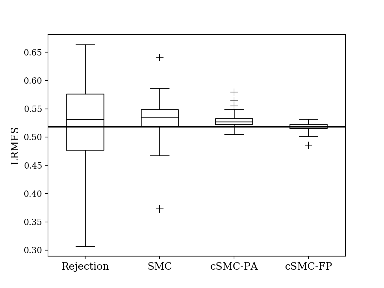
Figure 7: Boxplots of 100 independent estimates of LRMES using different methods. The horizontal line is the “true” LRMSE estimated using 100,000 samples generated by the rejection method.

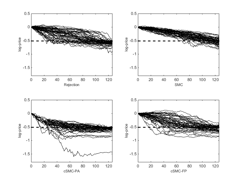
Figure 8: Sample paths of $X_{m,0:T}$ generated by different methods before weight adjustment. The horizontal line denotes a 40% price drop.

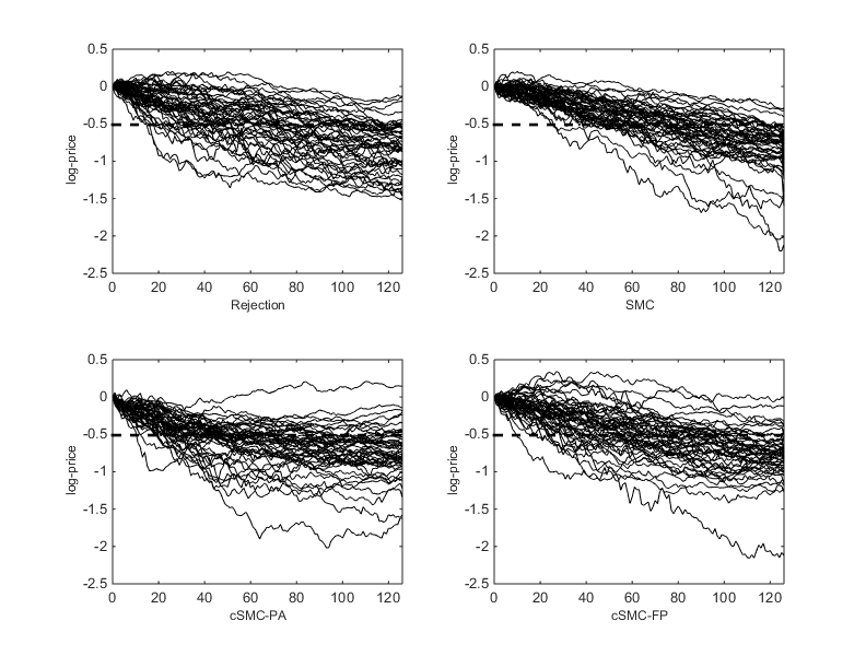
Figure 9: Sample paths of $x_{f,0:T}$ generated by different methods before weight adjustment. The horizontal line denotes a 40% price drop.

5.2 System with Intermediate Observations

Consider a diffusion process $\{X_{\lambda}\}_{0\leq\lambda\leq 90}$ governed by the following stochastic differential equation (Beskos et al., 2006)

$$dX_{\lambda}=\sin(X_{\lambda}-\pi)d\lambda+dW_{\lambda},$$

where $W_{\lambda}$ is a standard Brownian motion. The continuous-time diffusion process can be discretized by inserting intermediate time points with interval $\delta$. Let $x_{t}=X_{t\delta}$ for $t=0,1,\cdots,T$ with $T=90/\delta$. Using the Euler-Maruyama approximation, we have

$$x_{t}=x_{t-1}+\delta\sin(x_{t-1}-\pi)+\varepsilon_{t},$$ (18)

where $\varepsilon_{t}\sim N(0,\delta)$. We take $\delta=0.1$ in this example.

In this simulation study, two noisy observations of $X_{\lambda}$ are made at times $\lambda=30$ and $\lambda=60$. That is,

$$Y_{30}\sim N(X_{30},\sigma^{2})\quad\text{and}\quad Y_{60}\sim N(X_{60},\sigma^{2}).$$

We also fix the two endpoints at $X_{0}=a$ and $X_{90}=b$. The discretized time points $T_{0}=0$, $T_{1}=30/\delta$, $T_{2}=60/\delta$ and $T_{3}=90/\delta$ are considered to have strong constraints. The cSMC-BP method is applied to generate sample paths of $x_{0:T}$ conditional on the constraints $(X_{0},Y_{30},Y_{60},X_{90})$. That is, we use cSMC in Figure 1 to generate samples, and the backward pilot smoothing algorithm in Figure 6 is used to compute the resampling priority scores. We take equation (18) as the proposal distribution in generating forward paths. The backward pilots are generated according to the algorithm in Figure 6 with the proposal distribution $r(\widetilde{x}_{t}\mid\widetilde{x}_{t+1})\sim N\big{(}\widetilde{x}_{t+1}-\delta\sin(\widetilde{x}_{t+1}-\pi),\delta\big{)}$. Resampling is conducted dynamically when the ESS in (4) is less than $0.3n$. In this example, the time line is split into three segments. The segmental sampling procedure is demonstrated in Figure 10.

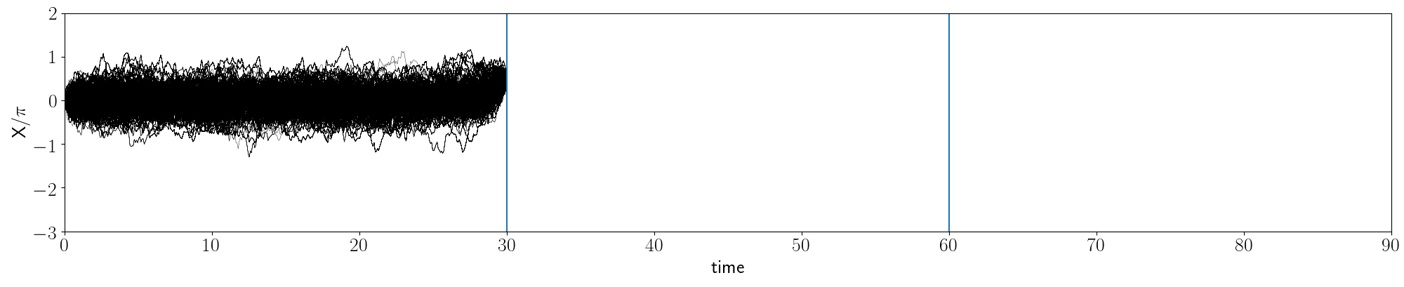
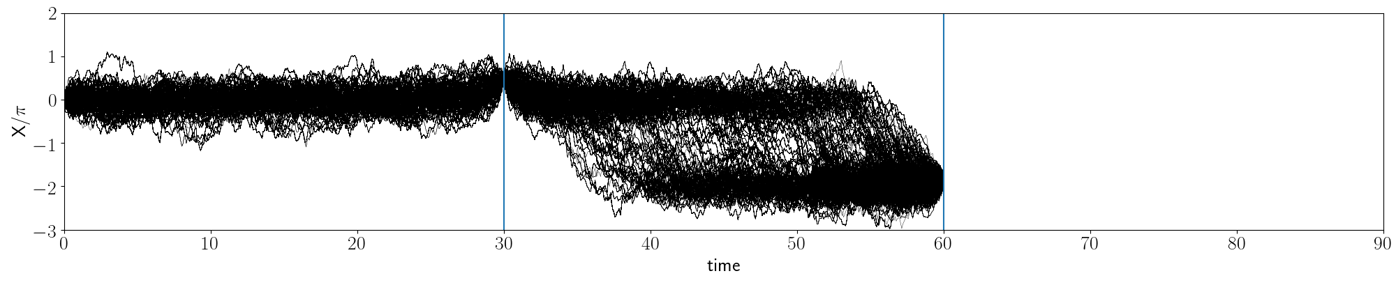
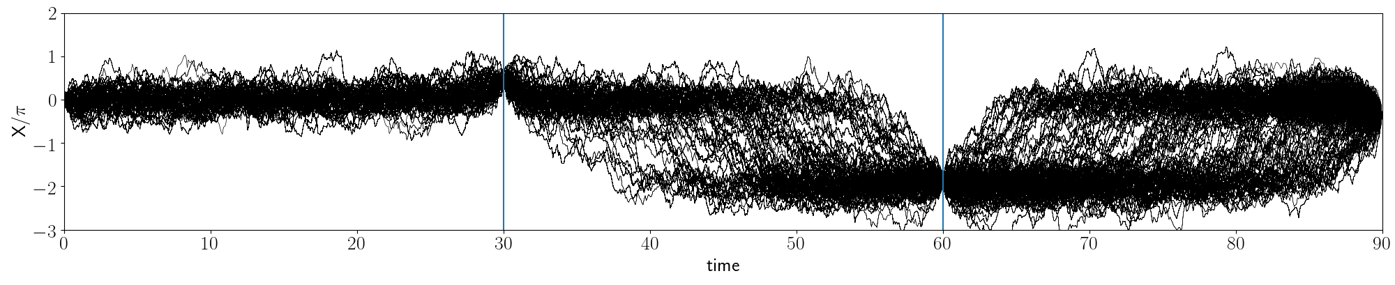
Figure 10: Illustration of the segmental sampling procedure.

In the first experiment, we set $X_{0}=0$, $Y_{30}=1.49$, $Y_{60}=-5.91$ and $X_{90}=-1.17$. Note that this process shows a jump behavior among the stable levels at $X_{\lambda}=2k\pi$, $k=0,\pm 1,\pm 2,\cdots$ (Lin et al., 2010). The four observations correspond to the stable levels 0, 0, $-2\pi$ and 0 accordingly. The process is likely to fluctuate around the stable level 0 during the first period. Then, it jumps to stable level $-2\pi$ in the second period and eventually jumps back to stable level 0 in the third period.

Three levels of measurement errors for the observations $Y_{30}$ and $Y_{60}$ are investigated: $\sigma=0.01$ for very accurate observations, $\sigma=1$ for moderate accurate observations and $\sigma=2$ for untrusted observations. Note that in this experiment we fix the observations $Y_{30}$ and $Y_{60}$ but changes the underlying assumption of their distributions to reflect the strength and accuracy of the observations. A total number of $1,000$ forward paths are generated, and $300$ backward pilots are used to estimate the resampling priority scores. Figure 11 plots the generated sample paths before weight adjustment for each level of error. Figure 12 shows the histogram of the marginal samples of $X_{60}=x_{60/\delta}$ before weight adjustment, which is obtained from the generated sample set $\{x_{0:T}^{(i)}\}_{i=1,\cdots,n}$ without considering the weights. It can be seen that when the observations are accurate ($\sigma=0.01$), the two observations act like fixed-point constraints that force all sample paths to pass through the observations. When the observation error is large ($\sigma=2$), a high proportion of sample paths remains at the original stable level while only a small proportion of paths is drawn towards the observations. The moderate error case ($\sigma=1$) is a compromise between these two cases. The marginal distributions of $X_{60}$ show clear differences in the above three cases. Samples from all three levels of error retain the jumping nature of underlying process and the cSMC-BP approach is capable of dealing with different levels of observational errors.

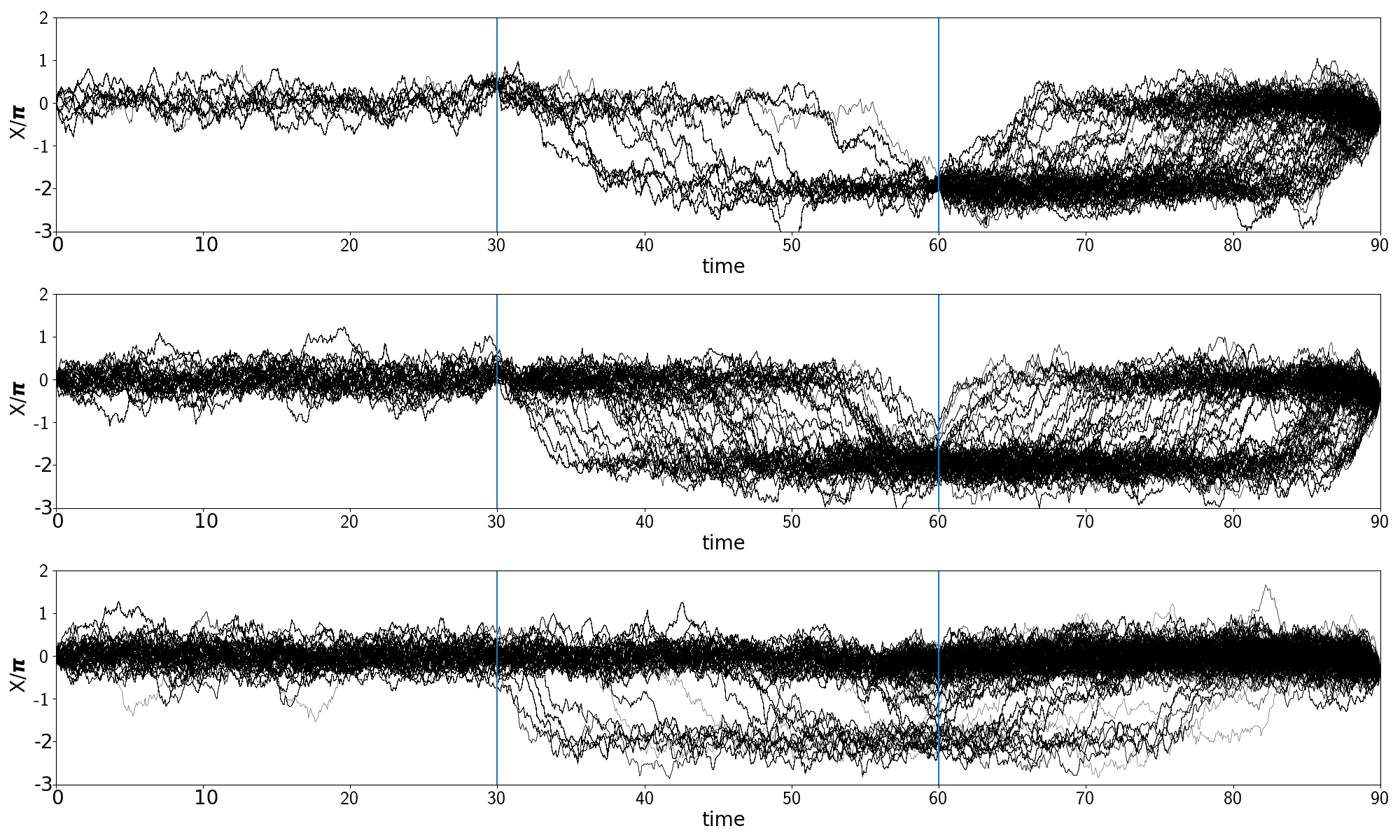
Figure 11: Sampled paths before weight adjustment for $\sigma=0.01$ (top panel), $\sigma=1.0$ (middle panel) and $\sigma=2.0$ (bottom panel) when $X_{0}=0$, $Y_{30}=1.49$, $Y_{60}=-5.91$ and $X_{90}=-1.17$

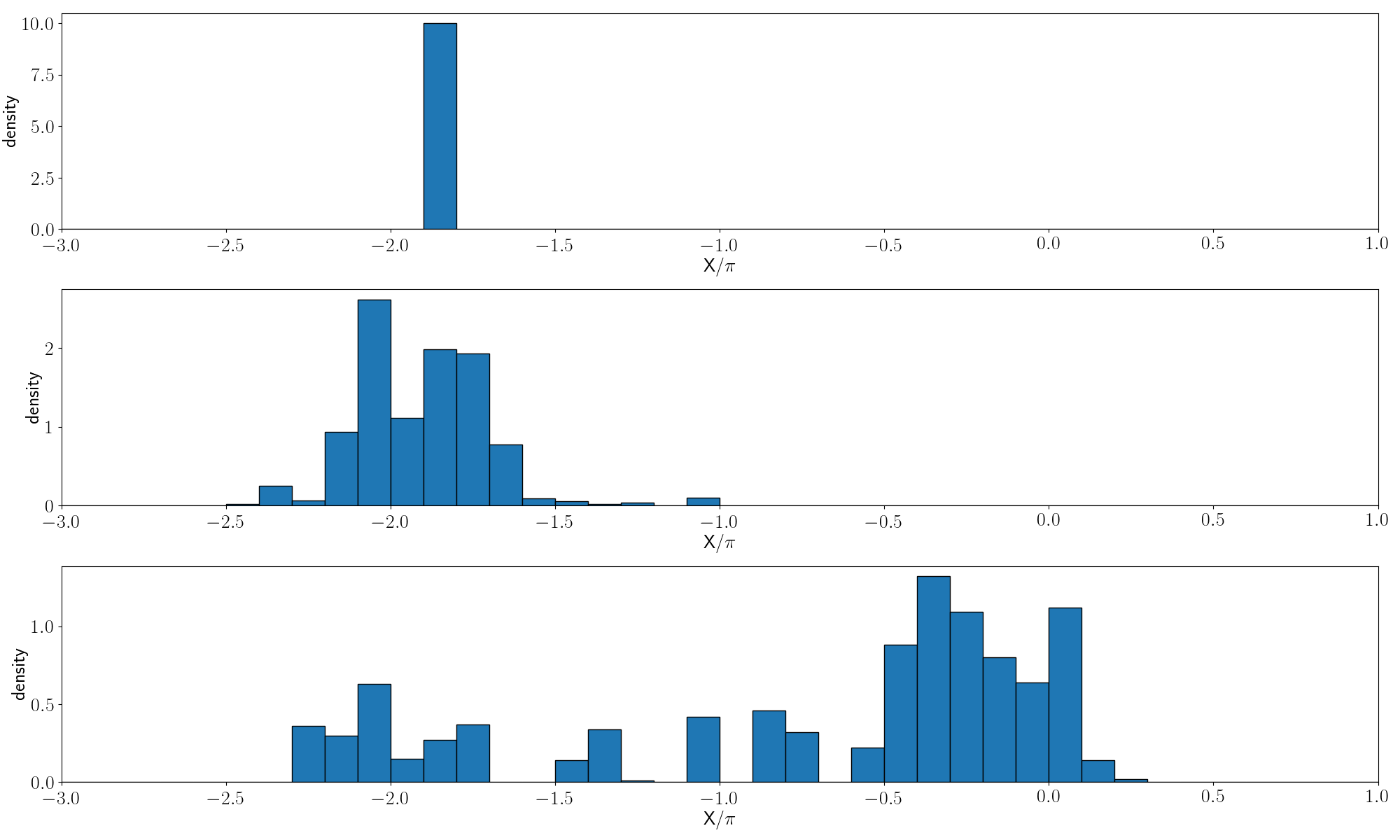
Figure 12: Histogram of the marginal samples of $X_{60}$ before weight adjustment for $\sigma=0.01$ (top panel), $\sigma=1.0$ (middle panel) and $\sigma=2.0$ (bottom panel) when $X_{0}=0$, $Y_{30}=1.49$, $Y_{60}=-5.91$ and $X_{90}=-1.17$.

Next, we use the same settings as above except that setting $Y_{30}=6.49$. Now the four observations $X_{0}=0$, $Y_{30}=6.49$, $Y_{60}=-5.91$ and $X_{90}=-1.17$ correspond to the stable levels 0, $2\pi$, $-2\pi$ and $0$, respectively. Since $Y_{30}$ and $Y_{60}$ differ by a gap of two stable levels, this is a very rare event. In this case, the Monte Carlo sample size is increased to 5,000 in order to overcome the degeneracy and to capture the rare event. Sample paths before weight adjustment and histograms of $X_{60}$ samples for different levels of error are shown in Figures 13 and Figures 14, respectively. In the large error case ($\sigma=2$), most samples are concentrated around the stable level 0. As the error level decreases, the observation induced constraints become stronger, hence more sample paths are drawn towards the observations. Those figures provide the evidence that the priority scores estimated by the backward pilots are effective for different error levels under this extreme setting.

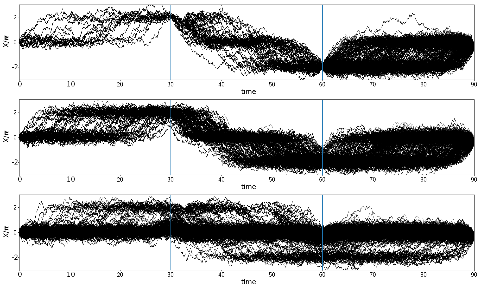
Figure 13: Sampled paths before weight adjustment for $\sigma=0.01$ (top panel), $\sigma=1.0$ (middle panel) and $\sigma=2.0$ (bottom panel) when $X_{0}=0$, $Y_{30}=6.49$, $Y_{60}=-5.91$ and $X_{90}=-1.17$.

Figure 14: Histogram of the marginal samples of $X_{60}$ before weight adjustment for $\sigma=0.01$ (top panel), $\sigma=1.0$ (middle panel) and $\sigma=2.0$ (bottom panel) when $X_{0}=0$, $Y_{30}=6.49$, $Y_{60}=-5.91$ and $X_{90}=-1.17$.

5.3 Sampling Constrained Trading Paths

In asset portfolio management, the optimal trading path problem is a class of optimization problems which typically maximizes certain utility function of the trading path (Markowitz, 1959). This optimization problem is often complicated, especially when trading costs are considered. Kolm and Ritter (2015) turned such an optimization problem into a state space model and explored Monte Carlo methods to numerically solve it.

More specifically, let $x_{0:T}=(x_{0},x_{1},\dots,x_{T})$ be a trading path where $x_{t}$ represents the holding position of an asset in shares at time $t$. In practice, a starting position $x_{0}$ and a target end position $x_{T}$ are often imposed for optimal execution of a large order with minimum market impact. Without loss of generality, we impose two endpoints at $x_{0}=0$ and $x_{T}=0$, respectively. Then it becomes an optimization problem to maximize the utility function

$$u(x_{0:T})=-\sum_{t=1}^{T}c_{t}(x_{t}-x_{t-1})-\sum_{t=1}^{T-1}h_{t}(y_{t}-x_{t})$$ (19)

given $x_{0}=0$ and $x_{T}=0$, where $(y_{1},y_{1},\dots,y_{T-1})$ is a predetermined optimal trading path in an ideal world without trading costs, typically obtained by maximizing the risk-adjusted expected return under the Markowitz mean-variance theory (Markowitz, 1959). Here $c_{t}(\cdot)$ is the trading cost function and $h_{t}(\cdot)$ stands for the utility loss due to the departure of the realized path from the ideal path. An emulating state space model can be implemented with the state equation $p(x_{t}\,|\,x_{t-1})\propto\exp\{-c_{t}(x_{t}-x_{t-1})\}$ and the observation equation $p(y_{t}\,|\,x_{t})\propto\exp\{-h_{t}(y_{t}-x_{t})\}$. The joint posterior distribution of such a state space model is

$$p(x_{1:T-1}\,|\,x_{0},y_{1:T-1},x_{T}) \propto \prod_{t=1}^{T}p(x_{t}\,|\,x_{t-1})\prod_{t=1}^{T-1}p(y_{t}\,|\,x_{t})$$ (20)

$$\propto \exp\left\{-\left[\sum_{t=1}^{T}c_{t}(x_{t}-x_{t-1})+\sum_{t=1}^{T-1}h_{t}(y_{t}-x_{t})\right]\right\}.$$

Thus, it is a state space model with fixed point constraints as described in Section 3.4.

Following Kolm and Ritter (2015), we set $T=20$. The ideal trading path is given by

$$y_{t}=25\exp\{-(t+1)/8\}-40\exp\{-(t+1)/4\}.$$

The trading cost function and the utility loss due to tracking error are set to

$$c_{t}(x_{t}-x_{t-1})=\frac{1}{2\sigma_{x}^{2}}\big{[}(x_{t}-x_{t-1})^{2}+2\alpha|x_{t}-x_{t-1}|\big{]}\quad\text{and}\quad h_{t}(y_{t}-x_{t})=\frac{1}{2\sigma_{y}^{2}}(y_{t}-x_{t})^{2},$$ (21)

respectively, where $\sigma_{x}^{2}=0.25$ and $\sigma_{y}^{2}=1$. Here the trading cost is assumed to be a quadratic function of the trade size $|x_{t}-x_{t-1}|$, and $\alpha$ is a non-negative constant related to volatility and liquidity of the asset (Kyle and Obizhaeva, 2011), which we will specify in the following.

It can be seen that maximizing the utility function (19) is equivalent to find the maximize-a-posterior (MAP) path of distribution (20). We use a two-step method to find the optimal trading path. First, we draw samples from the highly constrained conditional distribution (20) with the settings specified in (21). Then we discretize the space of $x_{t}$, $t=1,\cdots,T-1$, based on the generated sample paths. The Viterbi algorithm (Viterbi, 1967; Forney, 1973) is applied to find an optimal path that maximizes the utility function (19) within the discretized state spaces. In general, the closer the generated sample paths are to the optimal one, the better trading path the Viterbi algorithm will produce.

We investigate two cases of $\alpha$ in (21): $\alpha=0$ and $\alpha=0.5$. In both cases, we compare the performance of cSMC-BP with a standard SMC. The state equation $p(x_{t}\,|\,x_{t-1})\propto\exp\{-c_{t}(x_{t}-x_{t-1})\}$ is used to generate forward paths in both methods. However, the standard SMC uses $\beta_{t}^{(i)}=w_{t}^{(i)}$ as the resampling priority scores, but cSMC-BP uses $\beta_{t}^{(i)}=w_{t}^{(i)}\widehat{p}(y_{t+1:T-1},x_{T}\,|\,x_{t}^{(i)})$ estimated by the backward pilot method in Figure 6 for resampling, which takes the future information into account. The backward pilots are generated from the proposal distribution

$$r(\widetilde{x}_{t}|\widetilde{x}_{t+1})\propto\exp\left\{-\frac{1}{2\sigma_{x}^{2}}\big{[}(\widetilde{x}_{t}-\widetilde{x}_{t+1})^{2}+2\alpha|\widetilde{x}_{t}-\widetilde{x}_{t+1}|\big{]}\right\}.$$

We use $m=300$ backward pilots and generate $n=2,000$ forward sample paths from cSMC-BP. For the purpose of comparison, the standard SMC draws $n=2,300$ forward paths such that both methods have a similar computational cost. In both methods, a resampling step is conducted when the ESS in (4) is less than $0.3n$.

5.3.1 Case 1: $\alpha=0$

It can be seen that the state space model is linear and Gaussian when $\alpha=0$. Hence, the Kalman filter (Kalman, 1960) can be applied to obtain an exact optimal solution. The sample paths generated from the standard SMC and cSMC-BP before weight adjustment, along with the exact optimal path and the 95% point-wise confidence intervals obtained by the Kalman filter are plotted in Figure 15. The samples from the standard SMC in the left panel have a much larger variance and most of them lie outside the 95% confidence region, while most samples from cSMC-BP in the right panel stay within the 95% confidence region. In cSMC-BP, the backward pilots bring the information from the future and guide the forward sample paths by resampling. On the other hand, without using any future information, the standard SMC sampler propagates blindly and suffers a large divergency between the sampling distribution and the target distribution in the end.

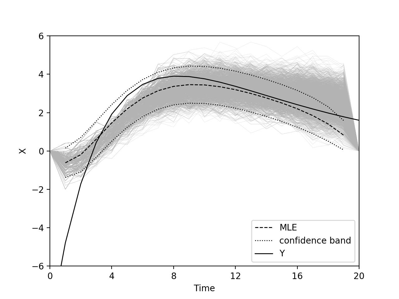
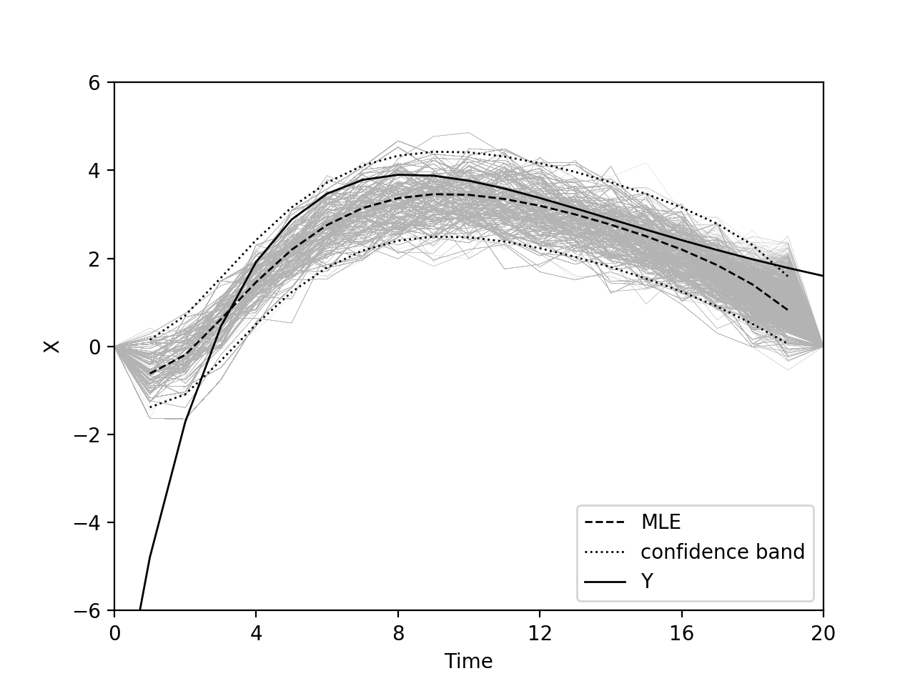
Figure 15: Sample paths from the standard SMC method (left panel) and from the cSMC-BP method (right panel) before weight adjustment when $\alpha=0$.

Figure 16 shows the marginal densities of the samples generated by the standard SMC and cSMC-BP before weight adjustment (left column) and after weight adjustment (right column) at time $t=4,12,19$. Both methods produce properly weighted samples, as the marginal densities for the samples after weight adjustment are close to the true one. However, the sampling distribution for $x_{19}$ before weight adjustment under the standard SMC method has a large divergence from the true distribution, which results in a low efficiency for inference.

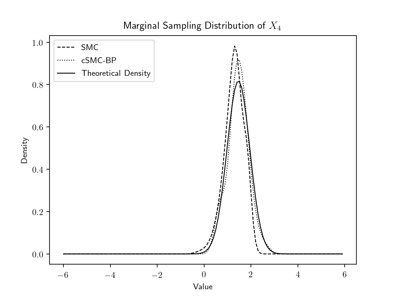
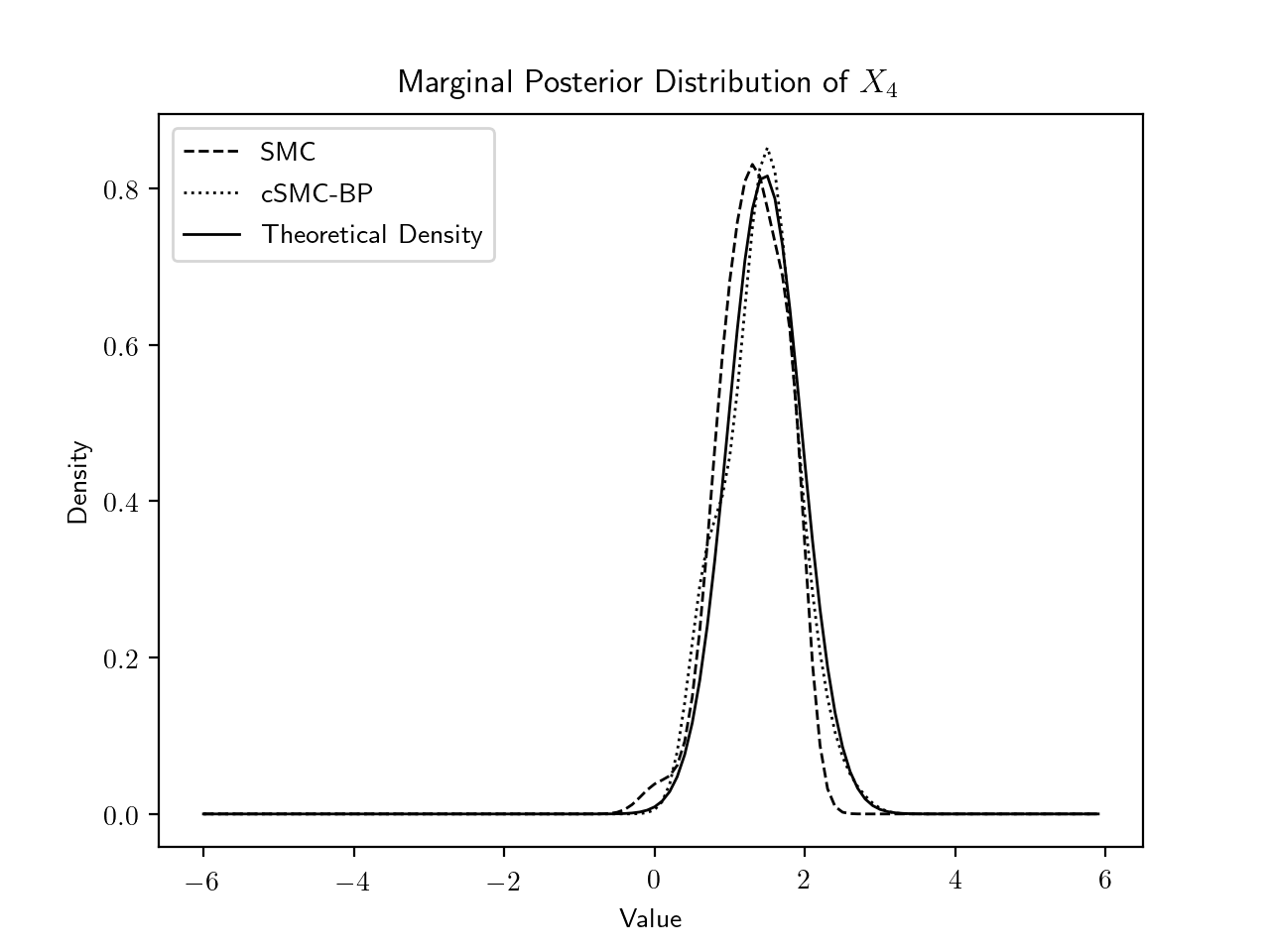
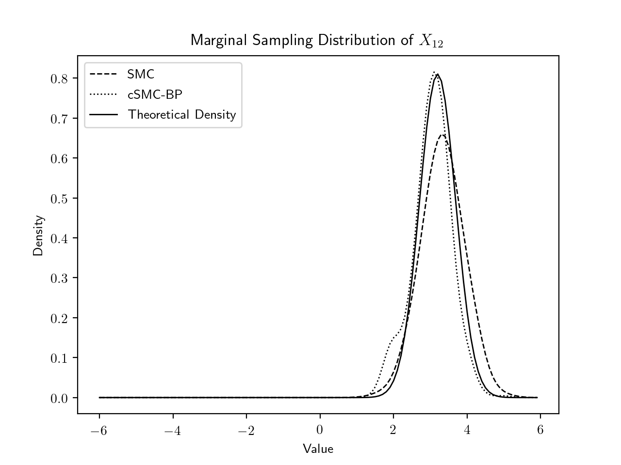
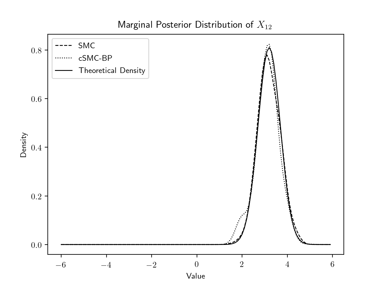
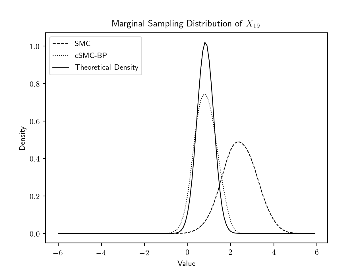
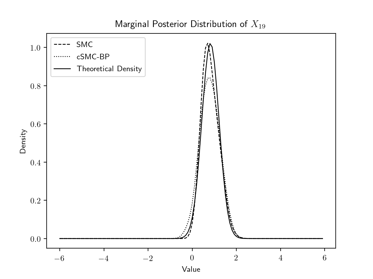
Figure 16: Marginal densities of the samples generated by SMC and cSMC-BP before weight adjustment (left column) and after weight adjustment (right column) at time $t=4$ (row 1), $t=12$ (row 2) and $t=19$ (row 3) when $\alpha=0$.

Figure 17 reports the mean squared errors (MSE) defined by

$$\text{MSE}(t)=\frac{1}{L}\sum_{l=1}^{L}\left[\widehat{E}^{[l]}(x_{t}\,|\,x_{0},y_{1:T-1},x_{T})-E(x_{t}\,|\,x_{0},y_{1:T-1},x_{T})\right]^{2},$$ (22)

where $E(x_{t}\,|\,x_{0},y_{1:T-1},x_{T})$ is the true conditional mean obtained from the Kalman filter, and $\widehat{E}^{[l]}(x_{t}\,|\,x_{0},y_{1:T-1},x_{T})$ is the conditional mean estimated by SMC or cSMC-BP in the $l$-th replication. We use $L=1,000$ replications to compute the MSE’s. It shows that in the period $8\leqslant t\leqslant 17$ where the fixed points have limited impacts, SMC and cSMC-BP have similar performance. But in the period $1\leqslant t\leqslant 7$ where the observation $y_{t}$ changes over time dramatically, cSMC-BP results in a smaller MSE than SMC as the future information is incorporated in its resampling step. In the period $t=18$ and $19$ where the end point constraint takes effect, the cSMC-BP approach also has a smaller MSE.

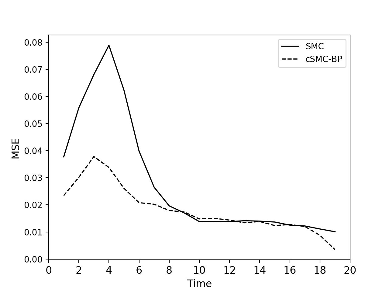
Figure 17: Mean squared error curves for SMC and cSMC-BP when $\alpha=0$.

5.3.2 Case 2: $\alpha=0.5$

When $\alpha=0.5$, the state space model is non-Gaussian, hence there is no analytic solution to maximize the utility function (19). In this case, we run a standard SMC sampling with $n=1,000,000$ sample paths to obtain the most likely sample path, the sample path with the largest likelihood value, together with 95% point-wise confidence intervals. The sample paths generated by SMC and cSMC-BP before weight adjustment, along with the most likely path and the 95% confidence region are plotted in Figure 18. Guided by the priority scores with future information, most samples generated by the cSMC-BP method stay within the 95% confidence region.

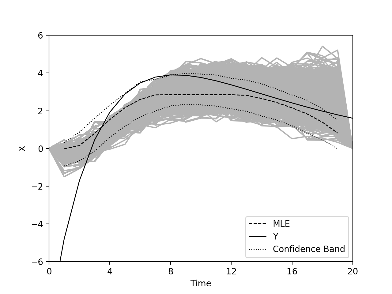
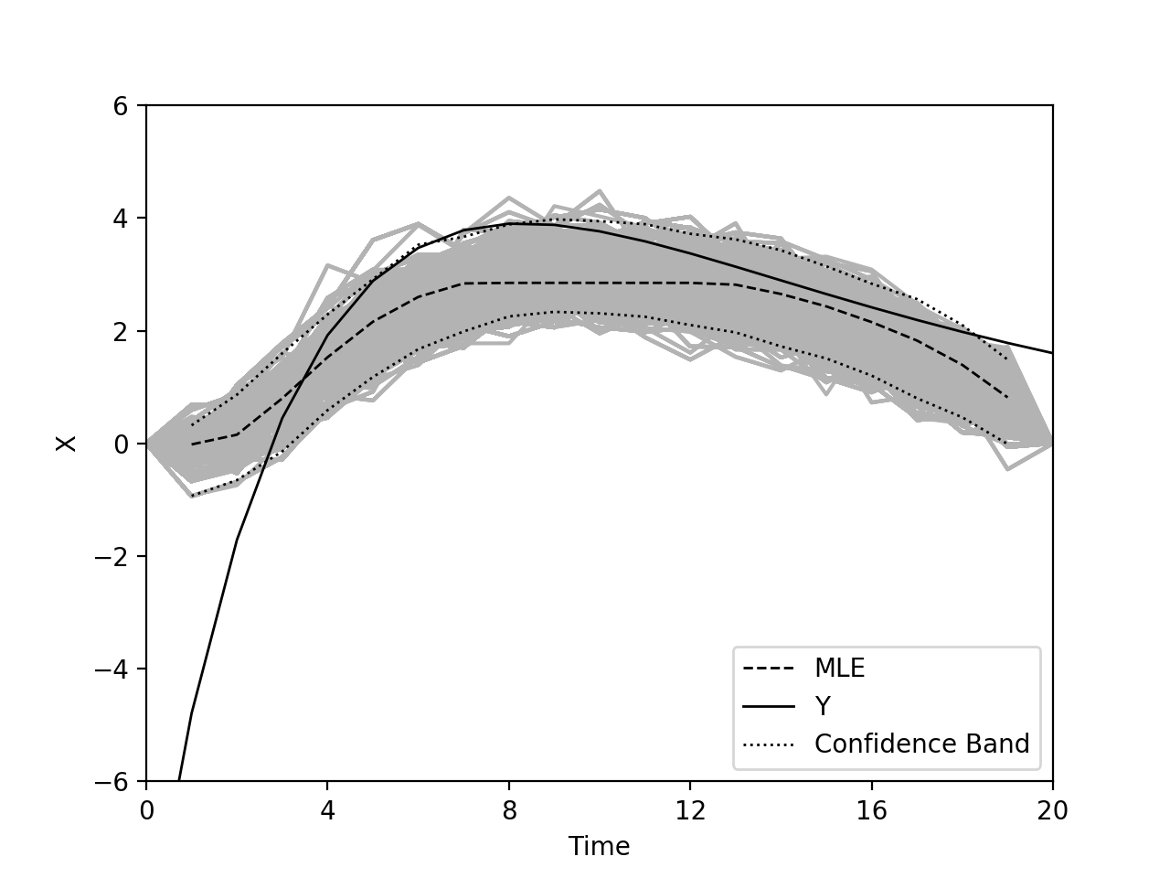
Figure 18: Sample paths from the standard SMC method (left panel) and from the cSMC-BP method (right panel) before weight adjustment when $\alpha=0.5$.

Figure 19 plots the marginal densities of the sample paths before weight adjustment (left column) and after weight adjustment (right column). The true marginal posterior distribution $p(x_{t}\,|\,x_{0},y_{1:T-1},x_{T})$ is estimated from the same $n=1,000,000$ SMC sample paths. At time $t=19$, the distribution of cSMC-BP samples is much closer to the target one than that of SMC samples. Figure 20 plots the MSE’s defined in (22). The results suggest that cSMC-BP reduces MSE at most times, especially in the periods $1\leqslant t\leqslant 7$ and $13\leqslant t\leqslant 19$.

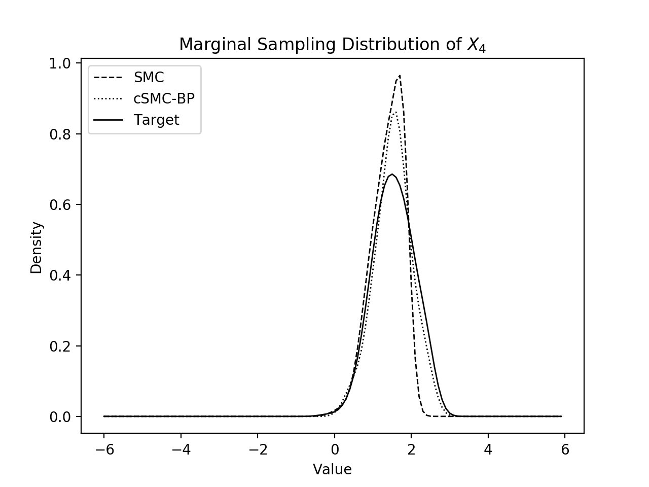
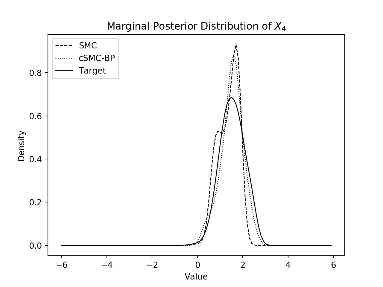
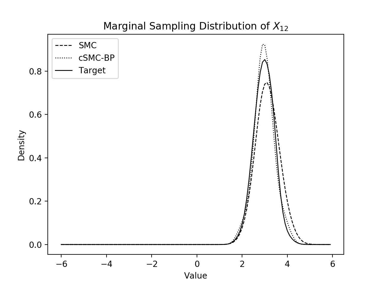
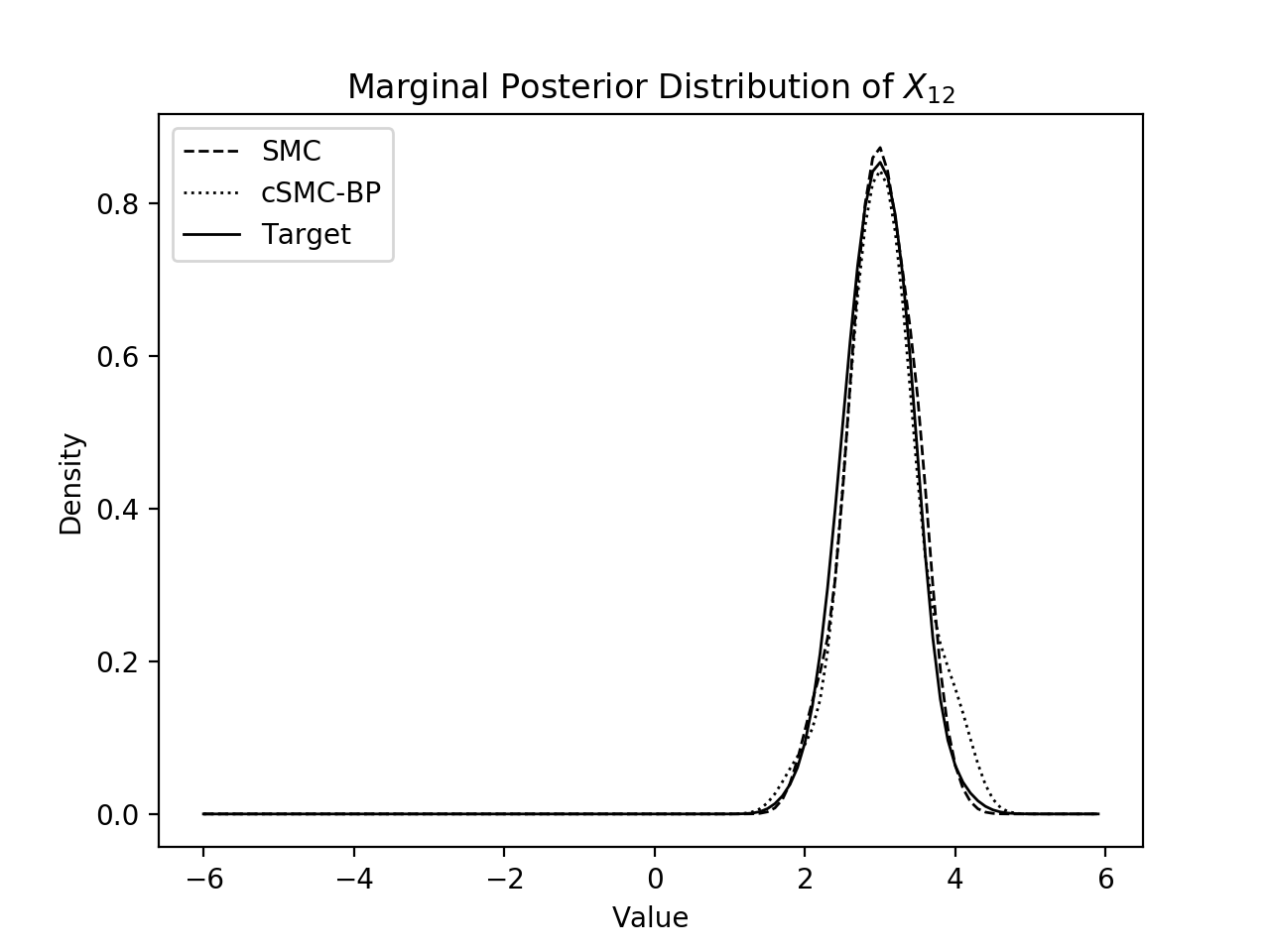
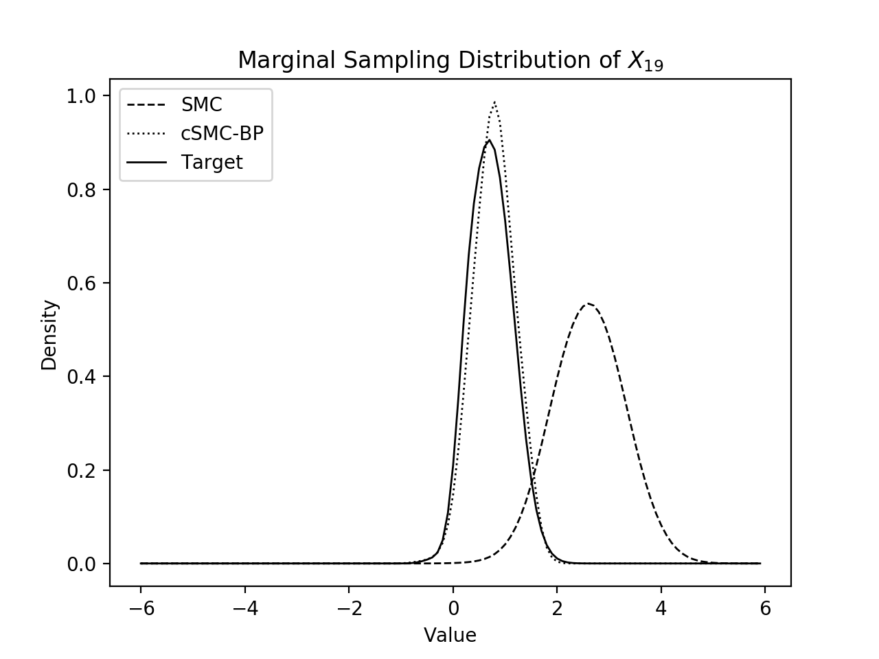
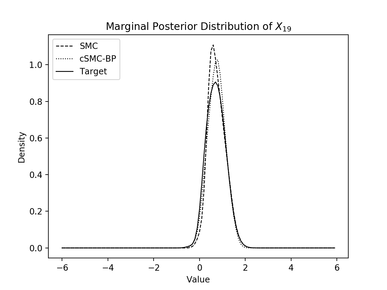
Figure 19: Marginal densities of the samples generated by SMC and cSMC-BP before weight adjustment (left column) and after weight adjustment (right column) at time $t=4$ (row 1), $t=12$ (row 2) and $t=19$ (row 3) when $\alpha=0.5$.

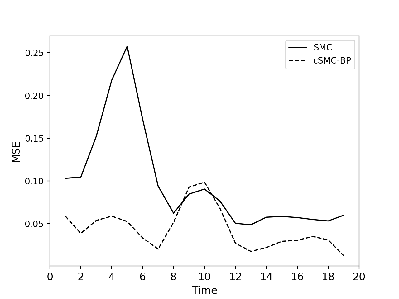
Figure 20: Mean squared error curves for SMC and cSMC-BP when $\alpha=0.5$.

5.3.3 Optimizing the Utility Function

The Viterbi algorithm (Viterbi, 1967; Forney, 1973) is a dynamic programming algorithm to find the most likely trajectory in a finite-state hidden Markov model. In this example, we discretize the state space based on the generated Monte Carlo state samples to utilize the Viterbi algorithm to find the optimal path and the optimal value of the utility function $u(x_{0:T})$ in (19). Specifically, given $\mathcal{X}_{t}=\{x_{t}^{(i)}\}_{i=1,\cdots,n}$ being the collection of samples of $x_{t}$ generated by SMC or cSMC-BP, the optimal path $(\hat{x}_{1},\cdots,\hat{x}_{T-1})$ is found by solving the following optimization problem

$$(\hat{x}_{1},\cdots,\hat{x}_{T-1})=\operatorname*{arg\,max}_{x_{1}\in\mathcal{X}_{1},\dots,x_{T-1}\in\mathcal{X}_{T-1}}u(x_{0:T})$$

with the Viterbi algorithm.

In this experiment, we use $m=300$ backward pilots and generate $n=500$ Monte Carlo forward samples from cSMC-BP. For comparison, $n=800$ samples are generated from the standard SMC method. The experiment is replicated 1,000 times. The optimal values of the utility function (up to a constant) solved by the Viterbi algorithm based on SMC samples and cSMC-BP samples respectively are reported in the boxplots in Figure 21. The true optimal value is marked by the horizontal lines. When $\alpha=0.0$, the true optimal value is obtained by the Kalman filter. When $\alpha=0.5$, the ”true” optimal value is computed by the Viterbi algorithm based on a large number ($n=10,000$) of SMC samples. Compared to the standard SMC method, the cSMC-BP method generates more samples around the true optimal path in the same amount of computation time by incorporating future information through resampling, hence it creates a better discrete state space for the Viterbi algorithm. As a result, the Viterbi algorithm based on cSMC-BP samples can produce trading paths with larger utility function values for both $\alpha=0$ and $\alpha=0.5$ cases.

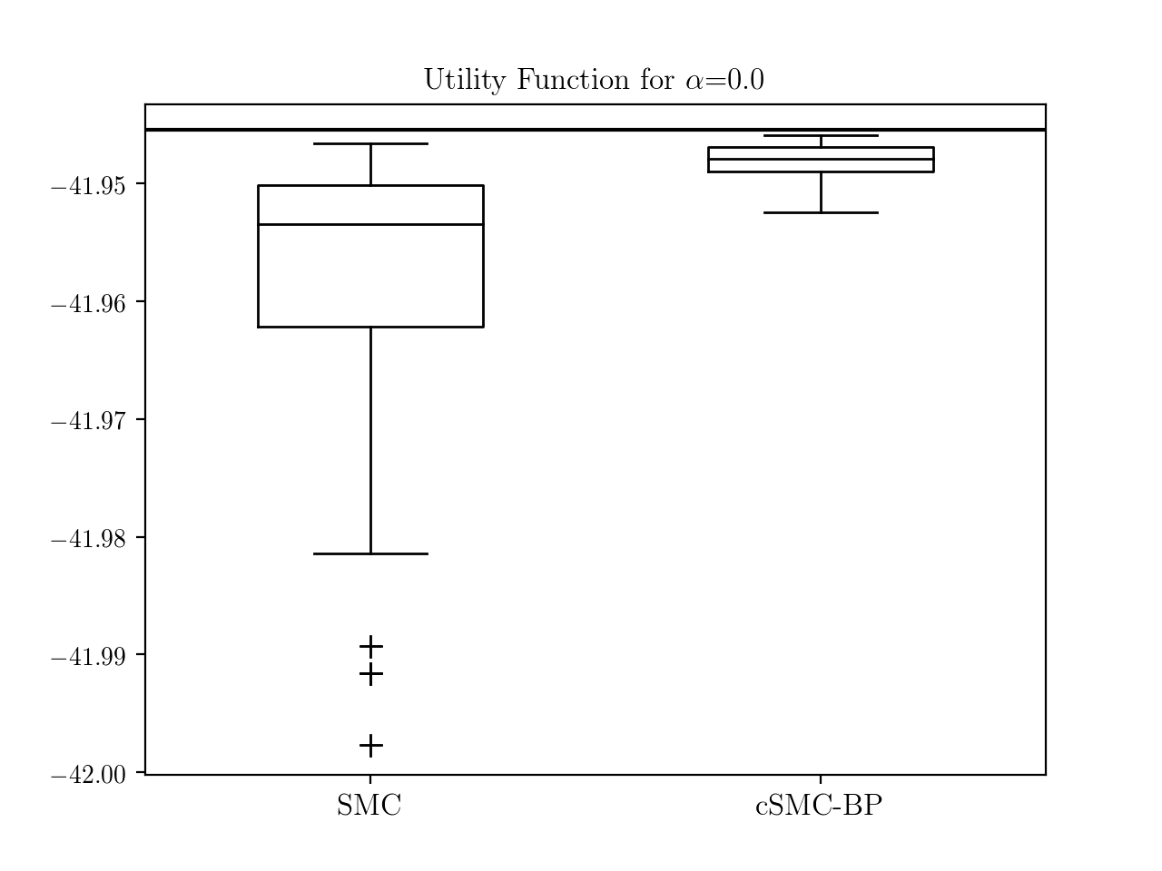
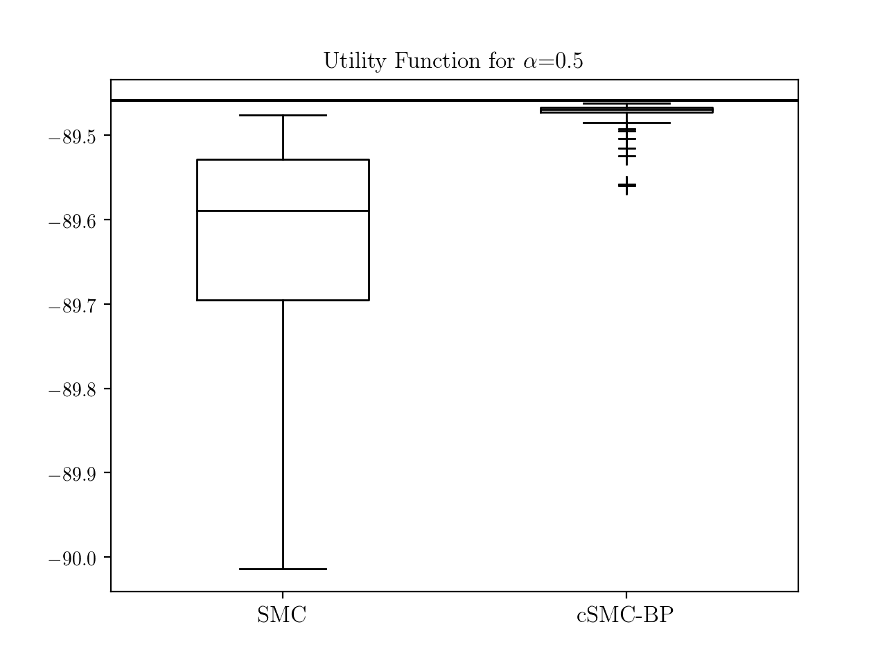
Figure 21: Boxplots of optimal values of utility function (19) solved by the Viterbi algorithm based on SMC samples and cSMC-BP samples when $\alpha=0$ (left panel) and $\alpha=0.5$ (right panel). The horizontal lines are the true optimal values.

6 Summary

In this article, we formulate the constrained sampling problem for general stochastic processes and proposed a general framework of cSMC algorithms. The key idea is to use the next available strong information $\mathcal{I}_{t_{+}}$ to adjust the sampling distribution at each intermediate point $t$ by choosing appropriate priority scores for resampling. We show that effective priority scores can be obtained from either forward pilot samples or backward pilot samples.

This framework is compatible with previous studies on state space model and diffusion bridge sampling problems as they can be viewed as special cases of the constrained sampling problems. The sampling procedure of cSMC coincides with the standard SMC approach for a state space model and Lin et al. (2010)’s algorithm in the diffusion bridge sampling problem.

Our framework can deal with a wider range of constraints. Three examples are demonstrated in Section 5: one with a subset constraint on the end point, one with noisy intermediate observation constraints and the other with multilevel constraints. These constraints go beyond the scope of fixed points, but can still be solved using cSMC.

Compared with the standard SMC algorithm, cSMC reduces the divergence between the sampling distribution and the true underlying target distribution by taking future information into consideration at each intermediate step. The additional computational cost is limited. Consequently, cSMC achieves a smaller estimation error with the same amount of computation time than the standard SMC implementation, as illustrated in the synthetic examples.

References

- Acharya et al. (2012) Acharya, V., Engle, R., and Richardson, M. (2012), “Capital shortfall: a new approach to ranking and regulating systemic risks,” American Economic Review: Papers & Proceedings, 102, 59–64.
- Avitzour (1995) Avitzour, D. (1995), “Stochastic simulation Bayesian approach to multitarget tracking,” IEE Proceedings-Radar, Sonar and Navigation, 142, 41–44.
- Beskos et al. (2006) Beskos, A., Papaspiliopoulos, O., Roberts, G. O., and Fearnhead, P. (2006), “Exact and computationally efficient likelihood-based estimation for discretely observed diffusion processes (with discussion),” Journal of the Royal Statistical Society: Series B (Statistical Methodology), 68, 333–382.
- Brownlees and Engle (2012) Brownlees, C. and Engle, R. (2012), “Volatility, correlation and tails for systemic risk measurement,” Tech. rep., SSRN 1611229.
- Chen et al. (2000) Chen, R., Wang, X., and Liu, J. S. (2000), “Adaptive joint detection and decoding in flat-fading channels via mixture Kalman filtering,” IEEE Transactions on Information Theory, 46, 2079–2094.
- Chen et al. (2005) Chen, Y., Xie, J., and Liu, J. S. (2005), “Stopping-time resampling for sequential Monte Carlo methods,” Journal of the Royal Statistical Society: Series B (Statistical Methodology), 67, 199–217.
- Doucet et al. (2006) Doucet, A., Briers, M., and Sénécal, S. (2006), “Efficient block sampling strategies for sequential Monte Carlo methods,” Journal of Computational and Graphical Statistics, 15, 693–711.
- Doucet et al. (2001) Doucet, A., De Freitas, N., and Gordon, N. (2001), “An introduction to sequential Monte Carlo methods,” in Sequential Monte Carlo Methods in Practice, Springer, pp. 3–14.
- Duan and Zhang (2016) Duan, J. and Zhang, C. (2016), “Non-Gaussian bridge sampling with an application,” Tech. rep., National University of Singapore.
- Durham and Gallant (2002) Durham, G. B. and Gallant, A. R. (2002), “Numerical techniques for maximum likelihood estimation of continuous-time diffusion processes,” Journal of Business & Economic Statistics, 20, 297–338.
- Fearnhead (2008) Fearnhead, P. (2008), “Computational methods for complex stochastic systems: a review of some alternatives to MCMC,” Statistics and Computing, 18, 151–171.
- Fong et al. (2002) Fong, W., Godsill, S. J., Doucet, A., and West, M. (2002), “Monte Carlo smoothing with application to audio signal enhancement,” IEEE Transactions on Signal Processing, 50, 438–449.
- Forney (1973) Forney, G. D. (1973), “The Viterbi algorithm,” Proceedings of the IEEE, 61, 268–278.
- Godsill et al. (2004) Godsill, S. J., Doucet, A., and West, M. (2004), “Monte Carlo smoothing for nonlinear time series,” Journal of the American Statistical Association, 99, 156–168.
- Gordon et al. (1993) Gordon, N. J., Salmond, D. J., and Smith, A. F. (1993), “Novel approach to nonlinear/non-Gaussian Bayesian state estimation,” IEE Proceedings F (Radar and Signal Processing), 140, 107–113.
- Kalman (1960) Kalman, R. E. (1960), “A new approach to linear filtering and prediction problems,” Journal of Basic Engineering, 82, 35–45.
- Kim et al. (1998) Kim, S., Shephard, N., and Chib, S. (1998), “Stochastic volatility: likelihood inference and comparison with ARCH models,” The Review of Economic Studies, 65, 361–393.
- Kitagawa (1996) Kitagawa, G. (1996), “Monte Carlo filter and smoother for non-Gaussian nonlinear state space models,” Journal of Computational and Graphical Statistics, 5, 1–25.
- Kolm and Ritter (2015) Kolm, P. N. and Ritter, G. (2015), “Multiperiod portfolio selection and bayesian dynamic models,” Risk, available at SSRN: https://ssrn.com/abstract=2472768.
- Kong et al. (1994) Kong, A., Liu, J. S., and Wong, W. H. (1994), “Sequential imputations and Bayesian missing data problems,” Journal of the American statistical association, 89, 278–288.
- Kyle and Obizhaeva (2011) Kyle, A. and Obizhaeva, A. (2011), “Market microstructure invariants: Theory and implications of calibration,” Available at SSRN: https://ssrn.com/abstract=1978932.
- Lin et al. (2013) Lin, M., Chen, R., and Liu, J. S. (2013), “Lookahead strategies for sequential Monte Carlo,” Statistical Science, 28, 69–94.
- Lin et al. (2010) Lin, M., Chen, R., and Mykland, P. (2010), “On generating Monte Carlo samples of continuous diffusion bridges,” Journal of the American Statistical Association, 105, 820–838.
- Lin et al. (2008) Lin, M., Lu, H.-M., Chen, R., and Liang, J. (2008), “Generating properly weighted ensemble of conformations of proteins from sparse or indirect distance constraints,” The Journal Of Chemical Physics, 129,094101, 1–13.
- Lin et al. (2005) Lin, M. T., Zhang, J. L., Cheng, Q., and Chen, R. (2005), “Independent particle filters,” Journal of the American Statistical Association, 100, 1412–1421.
- Liu (2001) Liu, J. S. (2001), Monte Carlo Strategies in Statistical Computing, Springer, New York.
- Liu and Chen (1995) Liu, J. S. and Chen, R. (1995), “Blind deconvolution via sequential imputations,” Journal of the American Statistical Association, 90, 567–576.
- Liu and Chen (1998) — (1998), “Sequential Monte Carlo methods for dynamic systems,” Journal of the American statistical association, 93, 1032–1044.
- Markowitz (1959) Markowitz, H. (1959), “Portfolio Selection, Cowles Foundation Monograph No. 16,” John Wiley, New York, 32, 263–74.
- Pedersen (1995) Pedersen, A. R. (1995), “Consistency and asymptotic normality of an approximate maximum likelihood estimator for discretely observed diffusion processes,” Bernoulli, 257–279.
- Pitt and Shephard (1999) Pitt, M. K. and Shephard, N. (1999), “Filtering via simulation: auxiliary particle filters,” Journal of the American statistical association, 94, 590–599.
- Scharth and Kohn (2016) Scharth, M. and Kohn, R. (2016), “Particle efficient importance sampling,” Journal of Econometrics, 190, 133–147.
- Viterbi (1967) Viterbi, A. (1967), “Error bounds for convolutional codes and an asymptotically optimum decoding algorithm,” IEEE Transactions on Information Theory, 13, 260–269.
- Wang et al. (2002) Wang, X., Chen, R., and Guo, D. (2002), “Delayed-pilot sampling for mixture Kalman filter with application in fading channels,” IEEE Transactions on Signal Processing, 50, 241–254.
- Zhang et al. (2007) Zhang, J., Lin, M., Chen, R., Liang, J., and Liu, J. S. (2007), “Monte Carlo sampling of near-native structures of proteins with applications,” Proteins: Structure, Function, and Bioinformatics, 66, 61–68.
- Zhang and Liu (2002) Zhang, J. L. and Liu, J. S. (2002), “A new sequential importance sampling method and its application to the two-dimensional hydrophobic–hydrophilic model,” The Journal of Chemical Physics, 117, 3492–3498.