Testing the simplifying assumption in high-dimensional vine copulas
Abstract
Testing the simplifying assumption in high-dimensional vine copulas is a difficult task. Tests must be based on estimated observations and check constraints on high-dimensional distributions. So far, corresponding tests have been limited to single conditional copulas with a low-dimensional set of conditioning variables. We propose a novel testing procedure that is computationally feasible for high-dimensional data sets and that exhibits a power that decreases only slightly with the dimension. By discretizing the support of the conditioning variables and incorporating a penalty in the test statistic, we mitigate the curse of dimensionality by looking for the possibly strongest deviation from the simplifying assumption. The use of a decision tree renders the test computationally feasible for large dimensions. We derive the asymptotic distribution of the test and analyze its finite sample performance in an extensive simulation study. An application of the test to four real data sets is provided.
doi:
10.1214/154957804100000000keywords:
1 Introduction
Vine copulas [24, 4, 1] are a popular tool to model multivariate dependence. An extensive literature concerning vine copulas has been based on the simplifying assumption [11, 19, 25, 28, 34]. This assumption states that every conditional copula in the vine copula does not vary in its conditioning arguments [21]. Multivariate distributions which can be represented as simplified vine copulas have been identified in early papers [21, 44]. More recently, the simplifying assumption has again attracted a lot of attention [10, 17, 18, 27, 32, 34, 43]. In the context of (bivariate) conditional copulas non- and semiparametric tests for the simplifying assumption have been developed [2, 17, 18]. See Derumigny and Fermanian [10] for a survey. In these studies the simplifying assumption is tested for one single conditional copula with a low-dimensional conditioning vector. The assumption is not tested for a vine copula where several conditional copulas with a possibly high-dimensional conditioning vector need to be checked.
We propose a framework for testing the simplifying assumption in high-dimensional vine copulas. By means of the partial vine copula, we introduce a novel stochastic interpretation of the simplifying assumption which is useful for testing it in high dimensions. We test the null hypothesis that the conditional correlation of the partial probability integral transforms associated with an edge of a vine is constant w.r.t. the conditioning variables. A rejection of this hypothesis implies that the simplifying assumption can be rejected as well. To obtain a test which is still powerful in high dimensions, we discretize the support of the conditioning variables into a finite number of subsets and incorporate a penalty in the test statistic. To render the test computationally feasible in high dimensions, we apply a decision tree to find the possibly largest difference in the set of conditional correlations. The test can be applied in high dimensions which is demonstrated in real data applications and in simulation studies with up to 12-dimensional data sets. An accompanying R-package pacotest [29] is publicly available and has been applied to even higher-dimensional data sets [27]. The test can be used to detect building blocks of a vine copula where the simplifying assumption does not seem to be adequate and the estimation of a conditional copula that is varying in its conditioning variables can improve the modeling [40]. It can also be applied to construct new methods for the structure selection of vine copulas [27].
The organization of the paper is as follows. The partial vine copula and stochastic interpretations of the simplifying assumption are discussed in Section 2. In Section 3 we present the test for constant conditional correlations and derive its asymptotic distribution. A decision tree algorithm for searching for the largest deviation from the simplifying assumption is proposed in Section 4. An extensive analysis of the finite sample performance of the test is provided in Section 5. In Section 6 a hierarchical procedure to test the simplifying assumption in vine copulas is presented and applied to simulated and real data. Concluding remarks are given in Section 7.
Throughout the paper we use the following notation and assumptions. The cdf of a -dimensional random vector is denoted by . The distribution function or copula of a random vector with uniform margins is denoted by . For simplicity, we assume that all random variables are real-valued and absolutely continuous. If and are stochastically independent we write . For the indicator function we use if is true, and otherwise. denotes the gradient w.r.t. and if is a -dimensional function then is the partial derivative w.r.t. the -th element. All proofs are deferred to the Appendix.
2 The partial vine copula and stochastic interpretations of the simplifying assumption
In this section, we first introduce concepts that are required for the remainder of this paper. Thereafter, we establish a new stochastic interpretation of the simplifying assumption to check its validity.
Let be a random vector where , are random variables and is a vector of dimension at least 1. For let , , and be the corresponding conditional distributions of , , and given , respectively.
Definition 1 (CPIT, bivariate conditional and partial copula)
While the bivariate conditional copula is the conditional distribution of a pair of uniform CPITs, the partial copula is the bivariate unconditional distribution of a pair of uniform CPITs. Sometimes, the function is constant for all , e.g., if the distribution of is multivariate normal. In this case, all conditional copulas , are equal to the partial copula . The bivariate conditional copula , of the bivariate conditional distribution arises if one expresses the cdf as follows
| (2.1) |
A complete decomposition of the corresponding multivariate copula into bivariate conditional copulas of bivariate conditional distributions is given by an R-vine copula. The underlying graphical structure of an R-vine copula is an R-vine.
Definition 2 (R-vine – Bedford and Cooke [3])
The sequence of trees is an R-vine on elements if
-
(i)
is a tree with nodes and set of edges .
-
(ii)
For : is a tree with nodes and set of edges .
-
(iii)
Proximity condition for : If two nodes in are joined by an edge, the nodes (being edges in ) must share a common node in .
The complete union associated with the edge in tree is defined as
The conditioning set of the edge in tree is given by and always consists of elements. The conditioned sets associated with the edge in tree are defined as and and are by construction singleton indices. We denote the set of all edges of the R-vine from tree on as so that the constraint set of the R-vine is given as .
The representation of a multivariate copula in terms of an R-vine copula arises if one assigns the corresponding bivariate copulas , of the bivariate distributions to the edges of the first tree and the corresponding bivariate conditional copulas , of the bivariate conditional distributions to the edges of higher trees [3]. Using (2.1) for uniform margins and multiple times for different dimensions of and taking all partial derivatives to get the density, the following 1 can be shown.
Proposition 1
(R-vine copula representation – Bedford and Cooke [3])
Let and be a uniform random vector with cdf .
Consider an R-vine structure (Definition 2).
Define for , and denote the conditional copula of by (Definition 1).
For we set with and .
The density of can be expressed as
In general, the estimation of an R-vine copula density is a difficult task if the dimension is not low. In order to simplify the modeling process and to overcome the curse of dimensionality, it is commonly assumed that the simplifying assumption holds for the data generating vine copula.
Assumption 1
1 characterizes the simplifying assumption in terms of restrictions that are placed on the functional form of bivariate conditional copulas of bivariate conditional distributions. That is, the simplifying assumption holds if each -dimensional111For , is a -dimensional function because it maps to a value of the density of the conditional distribution of given . function only depends on its first two arguments, but the other arguments have no effect for all edges , .
Note that the building blocks of the R-vine copula in 1 are determined by . The other way round, we can assign arbitrary bivariate conditional copulas to the edges of an R-vine to construct a multivariate copula. It is also possible to assign bivariate copulas to the edges of an R-vine to construct a multivariate copula. In this case, we call the resulting construction a simplified vine copula which is given as follows.
Definition 3
(Simplified vine copula (SVC) or pair-copula construction – Joe [23], Aas et al. [1])
Let and consider an R-vine structure .
For , let be a bivariate copula which we call a pair-copula.222We denote the building blocks
, of a simplified vine copula as pair-copulas to avoid any confusion with the bivariate copulas , in the first tree of the vine, or the
bivariate conditional copulas of bivariate conditional distributions in higher trees,
where is a conditional distribution of .
Let for .
For , , define
recursively as
| (2.2) |
with and where is selected such that .333 By the proximity condition of the R-vine (Definition 2) there exists a such that either or with and w.l.o.g. the definition in equation (2.2) is restricted to the first case – otherwise one can use the identity . The density of the resulting simplified vine copula is given by
Note that for , , in 3 is a function of 444It would be more explicit to write instead of . However, the shortened notation is commonly used in the vine copula literature and simplifies the notation. and that the density is specified by pair-copulas . From the second tree on, each of these pair-copulas, i.e., for , together with , specifies the conditional distribution of . Moreover, determines the bivariate conditional copula of the bivariate conditional distribution which is given by
If the data generating R-vine copula does not satisfy the simplifying assumption, a simplified vine copula can be used as an approximation. The partial vine copula is a special simplified vine copula which minimizes the Kullback-Leibler divergence from the data generating copula in a tree-wise fashion (Spanhel and Kurz [43]). Moreover, it gives rise to a stochastic interpretation of the simplifying assumption which is useful for testing the assumption in high dimensions. In order to define the partial vine copula (PVC) we have to construct partial probability integral transforms and higher-order partial copulas.
Definition 4
(Partial probability integral transforms and higher-order partial copulas – Spanhel and Kurz [43])
Let and be a uniform random vector with cdf .
Consider an R-vine structure (Definition 2).
For we define the first-order partial copula as
| (2.3) |
Define the partial probability integral transforms (PPITs) as for with and for , , as
| (2.4) |
with and where is selected such that .
For , , the -th order partial copula is defined as
| (2.5) |
Note that a first-order partial copula in (2.3) equals the corresponding partial copula for . However, a higher-order partial copula in (2.5) is, in general, not equal to the corresponding partial copula for , . The partial vine copula is now constructed by assigning the specific first-order and higher-order partial copulas to the edges of an R-vine.
Definition 5 (Partial vine copula (PVC) – Spanhel and Kurz [43])
Let and be a uniform random vector with cdf . Consider an R-vine structure (Definition 2). denotes the partial vine copula (PVC) of and its density is given by
where is the density of defined in (2.3) for and (2.5) for , . For we set .
To illustrate non-simplified vine copulas, simplified vine copulas and the partial vine copula, we consider a special case of Example 4.2 in Spanhel and Kurz [43]. For this purpose, let us introduce the following notation. If denotes a parametric copula family with dependence parameter and cdf we write , where , if for all . Moreover, , where is a bivariate copula with cdf , if for all .
Example 1
Let be the product copula with cdf and be the FGM copula with parameter and cdf . The building-blocks of the four-dimensional vine copula are chosen to be
The density of the data generating R-vine copula defined in Example 1 is given by
where the second equality holds because the copulas in the first and third tree are product copulas. For this data generating process, all building blocks of the vine copula are product copulas except for the second tree . In tree , both and depend on the conditioning variables and , respectively. Thus, the simplifying assumption does not hold. The building blocks of the non-simplified vine copula defined in Example 1 are illustrated in the left panel of Figure 1.
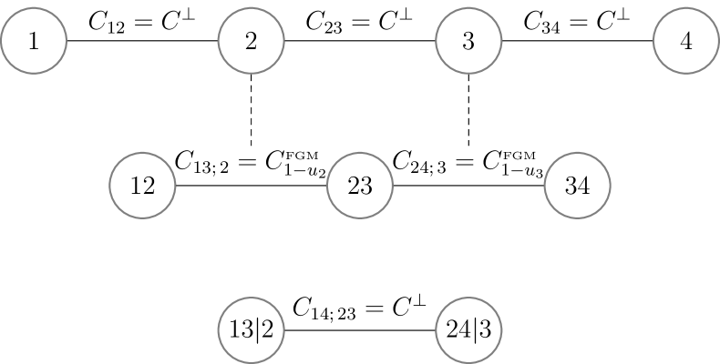
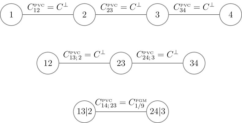
In order to approximate the non-simplified copula by a simplified vine copula one could assign arbitrary pair-copulas to the edges of the vine. For example the corresponding partial copulas. One can easily check that the partial copulas in the second tree are given by product copulas. Moreover, the partial copulas in the other trees are also given by product copulas. Thus, the resulting simplified vine copula model is the four-dimensional product copula with density given by
A better approximation, in terms of Kullback-Leibler divergence minimization, is given by the PVC (see Example 4.2 in Spanhel and Kurz [43]) with density
where the second equality holds because the copulas in the first and second tree of the PVC are product copulas. Note that the PVC approximates and in the second tree by the first-order partial copula which, by definition, always equals the partial copula. Thus, just like the previous approximation, the second tree is modeled by product copulas. However, the second-order partial copula in the third tree is a FGM copula with positive dependence and not equal to the corresponding partial copula , which is the product copula. Consequently, the four-dimensional approximation given by the PVC is not the four-dimensional product copula. The building blocks of the PVC corresponding to Example 1 are illustrated in the right panel of Figure 1.
The partial copula as well as the PVC give rise to the following stochastic interpretations of the simplifying assumption.
Theorem 1
(Stochastic interpretations of the simplifying assumption)
Let and be a uniform random vector.
Consider a fixed R-vine structure and the corresponding R-vine copula decomposition stated in 1.
The following statements are equivalent:
-
(i)
The R-vine copula satisfies the simplifying assumption (1).
-
(ii)
-
(iii)
1 highlights that the simplifying assumption is equivalent to vectorial independence assumptions. Note that in (ii) can be replaced by and that in (iii) can be replaced by . While the different stochastic interpretations (ii) and (iii) are equivalent in theory, (iii) is much more useful for testing the simplifying assumption. In practice, observations from the pair of CPITs or the pair of PPITs are not observable and have to be estimated from data. Observations from the CPIT can be obtained by estimating the -dimensional conditional distribution function of given , which is not an easy task. For , , the PPIT is a composition of pair-copulas which belong to the building blocks of the corresponding PVC given in equation (2.4) of 4. Thus, for observations from a PPIT one can sequentially estimate a sequence of pair-copulas which is much simpler. Therefore, we use (iii) to construct a test which is based on pseudo-observations from the PPITs.
To illustrate the practical advantage of testing the simplifying assumption with PPITs ((iii) in 1) instead of CPITs ((ii) in 1) let us reconsider Example 1. In this case, the simplifying assumption can be formulated either as
| or | |||
For the four-dimensional Example 1, both formulations (ii) and (iii) consist of three vectorial independencies, all of which must be true to be equivalent to the simplifying assumption, see 1. In tree , the required conditions are identical for both (ii) and (iii). Since the copulas in tree are given by bivariate FGM copulas with a varying parameter, these vectorial independencies do not hold. Thus, the simplifying assumption does not hold according to both (ii) and (iii). Note that the difference between (ii) and (iii) becomes only apparent after the second tree. In the third tree, the vectorial independencies stated in (ii) and (iii) are quite different. For the data generating vine copula (Example 1) the statement in tree is obviously true for (ii). However, it is false for (iii) because and, as can be readily verified, is false.
If the data generating vine copula is unknown, it is more practical to base a test on (iii) than on (ii). In order to check whether the pair of CPITs are jointly independent from in (ii), one has to estimate the unknown conditional distribution functions and . The specification of a flexible parametric model for such conditional distributions is difficult. Non-parametric estimation might be sensible if the conditioning vector is very low-dimensional but suffers from the curse of dimensionality if the conditioning vector is high-dimensional. On the other side, (iii) just requires the estimation of pair-copulas, irrespective of the dimension of the conditioning vector. That is because both PPITs can be written as a composition of pair-copulas. For instance,
so that only the estimation of and are required to estimate . In many applications, it might be feasible to find good parametric models for these pair-copulas in order to obtain an appropriate estimate of .
3 Constant conditional correlation (CCC) test for
Before we consider testing the simplifying assumption, we first develop in this and the next section tests for the null hypothesis for some . The main challenge is that the dimension of can be rather large so that the power of consistent tests is not satisfying in higher trees. For instance, a consistent test could be obtained using a Cramér-von Mises test for vectorial independence (Kojadinovic and Holmes [26] and Quessy [39]). However, as it is pointed out by Gijbels, Omelka and Veraverbeke [17] and shown in our simulation, the power of such a consistent test rapidly approaches the significance level if the dimension increases. Our focus is on a test that exhibits a power that is high for alternatives that one encounters in practical applications and that is quite robust to the dimension of the data set. For this reason, we consider the null hypothesis that the conditional correlation of the PPITs associated with one edge of a vine is constant w.r.t. the conditioning variables . A rejection of this hypothesis implies that the simplifying assumption can be rejected as well. To obtain a test whose power does not collapse substantially with the dimension of the conditioning vector, we now discretize the support of the conditioning vector into a finite number of subsets.
3.1 CCC test with known observations
For the ease of exposition, we introduce the main idea of the test without a reference to vine copulas. Let , be uniform random variables and be a random vector with uniform margins. We want to check the null hypothesis . Let , with , and with . We call a partition of the support of into two disjoint subsets.555The idea of discretization has some similarity to the boxes approach of Derumigny and Fermanian [10] but differs substantially. We only discretize the support of the conditioning vector and the rejection of our null hypothesis is still a rejection of the simplifying assumption which is not always true for the approach of Derumigny and Fermanian [10]. Moreover, we present a data-driven approach to select the partition so that the idea of discretization can also be applied in high-dimensional settings without the need to impose strong a priori assumptions on the form of the partition. We are interested in the correlation between and in the two subgroups determined by , i.e.,
for . Under , it follows that
i.e., the conditional correlations are constant w.r.t. the conditioning event. As estimate for the correlation in the -th group we use the sample version of the conditional correlation which we denote by .
A statistic for testing the equality of the correlations in the two samples is given by
where is a consistent estimator (see Section A.2) for the asymptotic variance of . By construction of the estimators, the asymptotic covariance between and is zero. Thus, under regularity conditions and it can be readily verified that .
In a more general setting, one can also use a partition of the support into pairwise disjoint subsets and test whether
For this purpose, denote the vector of sample correlations in the groups by . Further, define the diagonal matrix , with diagonal elements and a first-order difference matrix so that . A statistic to test the equality of correlations in groups is then defined by the quadratic form666 The statistic also follows from , where is the average correlation, is defined in Section A.2 as the fraction of data corresponding to the subset and with an appropriately defined matrix .
with asymptotic distribution under .
3.2 CCC test with estimated pseudo-observations from the PPITs
In order to test the simplifying assumption, we have to test null hypotheses of the form . In practice, if is the data generating process, we cannot directly observe a sample of but have to estimate such observations on the basis of a sample of . To obtain these pseudo-observations, we use a semi-parametric approach. First, we use normalized ranks to obtain pseudo-observations from for . We then consider a fixed R-vine structure and assume that there is a parametric simplified vine copula model for the PVC of with so that . Finally, we use the common stepwise ML estimator [20] to construct pseudo-observations from . The asymptotic distribution of the resulting test statistic with these estimated pseudo-observations is stated in Proposition 2.
Proposition 2
Let be independent copies of and be the copula of . Consider a fixed R-vine structure (Definition 2) and assume there is a parametric simplified vine copula model for the PVC of with so that . Let be fixed. Assume that the regularity conditions stated in Theorem 1 in Hobæk Haff [20] hold 777 Note that the results in Hobæk Haff [20] are written up for D-vine copulas but can be generalized to R-vine copulas [20]. The entries of the matrices needed to compute the standard errors of the sequentially estimated parameters of R-vine copulas can for example be found in Stöber and Schepsmeier [45].and that the partition , where , satisfies
-
(i)
, for with ,
-
(ii)
with for all .
Let be the vector of sample correlations that are computed using the pseudo-observations from the PPITs and where is defined in equation (A.8) in Section A.2. Construct the test statistic
| (3.1) |
Under it holds that
The matrices and quantify the change in the asymptotic covariance due to the estimation of pseudo-observations from the PPITs. If the marginal distributions are known and we don’t have to estimate ranks to obtain pseudo-observations from it follows that . If the PVC of is known it follows that . Note that, in general, the off-diagonal elements of , i.e., the asymptotic covariances between estimated correlations in different groups, are no longer zero if observations from the PPITs are estimated.
3.3 CCC test with a combination of partitions
The selected partition has an influence on how well a varying conditional correlation is detected by the test. To illustrate this and to motivate a test based on the combination of several partitions, we use the following Example 2.
Example 2
Let and be the Clayton and Frank copula with parameter , respectively. The building-blocks of the four-dimensional D-vine copula are chosen to be
with and , where is the value of Kendall’s of the bivariate margins in the first tree.888 The parameter function is a generalization of the function used by Acar, Craiu and Yao [2] for a Frank copula with a one-dimensional conditioning set, where the conditioning variable is assumed to be uniformly distributed on the interval . The parameters of the bivariate Clayton copulas in the first and second tree are specified in a way that Example 2 can be considered as a four-dimensional Clayton copula where the copula in the last tree is replaced by a Frank copula with varying parameter.
For the illustration we set in Example 2 and and simulate a sample of size . For instance, if we choose and , then and the power of the test is asymptotically equal to the level of the test. Instead, we could use partitions such as or . In Figure 2, we illustrate the resulting tests and .
The upper row corresponds to the first partition where the difference of the correlations in the two groups is , yielding a test statistic value of . In contrast, if we consider the second partition shown in the lower row of Figure 2, we get and .
In order to increase the probability that the test detects a varying conditional correlation, it seems naturally to consider several partitions , , where each partition is a collection of subsets of the support . A test statistic using a combination of partitions is given by
| (3.2) |
where is a penalty function and is the base partition whose corresponding test statistic is the only one that is not penalized. The construction of such a test has some similarity to the approach of Lavergne and Patilea [30]. The idea is that by choosing an appropriate penalty function, under , the asymptotic distribution of and should be equivalent. Moreover, if is not true, then should have more power than because, by construction, . Precise conditions are given in the following proposition.
Proposition 3
Assume that the conditions stated in Proposition 2 hold and that the partitions fulfill the conditions stated for in Proposition 2. Additionally, let be a penalty function such that
-
(i)
for ,
-
(ii)
for .
Set , where is defined like in equation (3.1) in Proposition 2 with replaced by . Under it holds that
where is the number of subsets of . If there is a partition , such that it follows that
Thus, the critical value of under asymptotically (as , for fixed ) only depends on the number of elements in but not on . In finite samples, however, the distribution of under also depends on and the usage of asymptotic critical values derived from the limiting distribution may result in an empirical size that is not close to the theoretical level.999 In extensive simulation studies in Section 5 and Section 6.1 it is demonstrated that the empirical size is often comparable to the theoretical level and the choice of the penalty function is analyzed in a simulation study in Appendix A.6 Moreover, if there is a partition such that the corresponding correlations are not identical, i.e., , the power of the test approaches 1 if the sample size goes to infinity. Possible choices of the partitions and their selection will be discussed in the next section.
4 A data-driven algorithm for testing with a high-dimensional conditioning vector
Both constant conditional correlation (CCC) tests, and , are based on partitions of . We will first illustrate why an a priori determination of such partitions is problematic and then show how such partitions can be selected in a data-driven fashion.
4.1 A priori defined partitions
As a naive approach one could use the sample median of each conditioning variable to split the observations into groups and then consider the partition that results from the combinations of these groups. For instance, for in the third tree, we obtain the following four subsets forming a partition
Such an approach is however only feasible for a low-dimensional conditioning vector, since the number of subsets increases exponentially with the dimension of the conditioning vector. Moreover, the number of observations that are contained in a single subset might get too small. Alternatively, one could use the mean of the conditioning variables for , , and consider the sample median of as split point to obtain the following partition of the support :
| (4.1) |
However, in practice, such an a priori definition of the partition is arbitrary and might not detect a conditional variation. Therefore, we introduce now a decision tree algorithm which selects the partitions in a more data-driven way and is computationally feasible in high dimensions.
4.2 Data-driven choice of the partitions by means of a decision tree algorithm
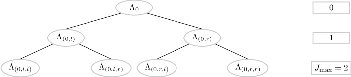
The test statistic can be rewritten in the following way
with . The set denotes the partition, excluding the base partition , for which a possible violation of the is most pronounced. As base partition we set (see equation (4.1)). To find in a data-driven and computationally efficient way we use decision trees with depth like the one shown in Figure 3. The decision tree recursively uses binary splits to partition the support into disjoint subsets to obtain . The possible split points in the first level are given by the empirical quartiles of each conditioning variable and by the empirical quartiles of the mean of the conditioning vector. In the second level, the split points for each leaf are chosen similarly but conditional on the chosen subsets of the first level. Among these possible splits the split is chosen that maximizes the statistic of the CCC test. For algorithmic details of the decision tree with a general depth of we refer to Section A.4.
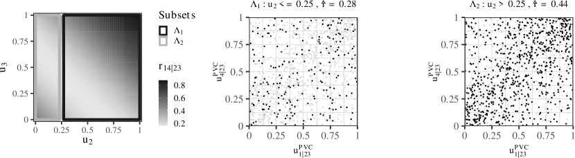
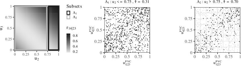
We revisit Example 2 to illustrate how the decision tree adapts to the variation in the conditional correlation. For the same simulated sample that is used for Figure 2, the decision tree is applied to test . The partitioning of into is visualized in Figure 4 which shows the grouping of the observations from the PPITs according to .
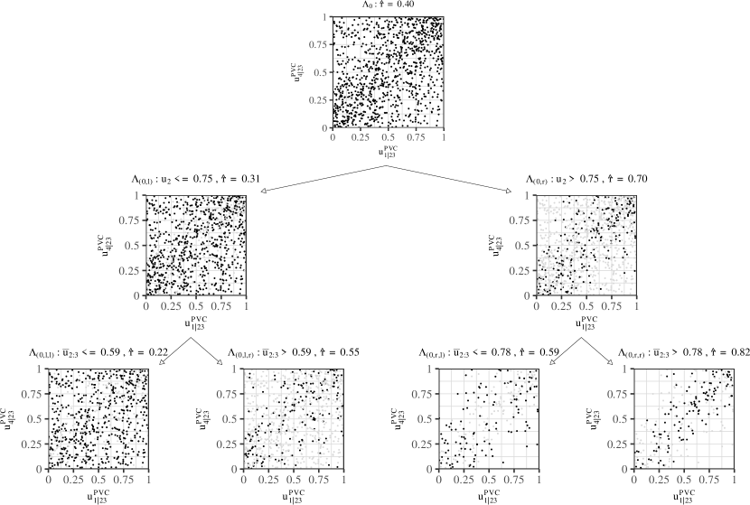
In each scatter plot the black observations have been assigned to this leaf while the observations in light gray have been assigned to the other leaf. Furthermore, the estimated correlations in each group, which are used for the CCC test, are shown. We see that the decision tree chooses a partition with estimated correlations that are quite different and a maximal difference of
| Subset | ||
| 0 | ||
| 1 | ||
| 1 | ||
| 2 | ||
| 2 | ||
| 2 | ||
| 2 |
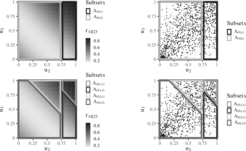
The subsets that are constructed by the decision tree to obtain the selected partition are stated in Table 1 together with the corresponding estimated correlations. The decision tree generates partitions which are no longer simple one-directional splits as in Figure 2. Instead we now get more complex polygons as subsets which are visualized as colored frames in Figure 5. On the left hand side of Figure 5, the shaded area shows the variation in the correlation of as a function of and . Areas with darker gray correspond to higher values of the conditional correlation . The right hand side of Figure 5 illustrates how the dependence within the conditioning set, determined by the Clayton copula , influences the variation of . Shown are the realized values of and their grouping into the subsets. The two plots on top correspond to the first binary split, which is done according to the 75% quartile of . The two plots at the bottom show the splits in the second level of the decision tree, which is done according to quartiles of the mean of the conditioning variables and . The adaption of the decision tree based partition to the variation in the conditional correlation becomes clear when looking at the shaded background which shows the conditional correlation of as a function of and . We see how is partitioned into areas with relatively low (), medium ( and ) and high correlation ().
In all simulations in Section 5 and Section 6.1, and the real data applications in Section 6.2, we use decision trees with depth and for the penalty. The choice of the penalty function is analyzed and explained in Appendix A.6. We further set (see equation (4.1)) as base partition, because we assume to have no a priori information about the relative importance of each conditioning variable and because the median of the mean of the conditioning vector as split point guarantees well-balanced sample sizes in the groups.101010 If the application at hand suggests a priori that is likely to be false and a particular partition would result in a more pronounced difference between the resulting conditional correlations, i.e., , then setting instead of would not deteriorate but possibly improve the power of the test provided is actually false. However, as it is shown in Section 5.2 the choice of is not crucial if the alternative partitions are selected in a data-driven way using the decision tree.
5 CCC test: Simulation study
In the following, the finite-sample performance of the CCC test is analyzed and compared to the performance of the vectorial independence (VI) test of Kojadinovic and Holmes [26]. The simulation study is build around Example 2 using a ceteris paribus setup in order to analyze the different key drivers of the empirical power. We will analyze the power of the CCC and the VI test w.r.t. different variations of the conditional copula in Section 5.1, illustrate the power gain of the CCC test due to the decision tree algorithm in Section 5.2, and investigate the performance of both tests w.r.t. the dimensionality of the testing problem in Appendix 5.3. The effect of misspecified copula families in lower trees is discussed in Section 5.4.
All results for the CCC test are computed with estimated pseudo-observations from the PPITs. Since the asymptotic distribution of the VI test with estimated pseudo-observations is unknown, we use the true observations from the PPITs for the VI test to compute p-values on the basis of 1000 bootstrap samples [39]. Therefore, in simulations with possible misspecifications we do not show results for the VI test.
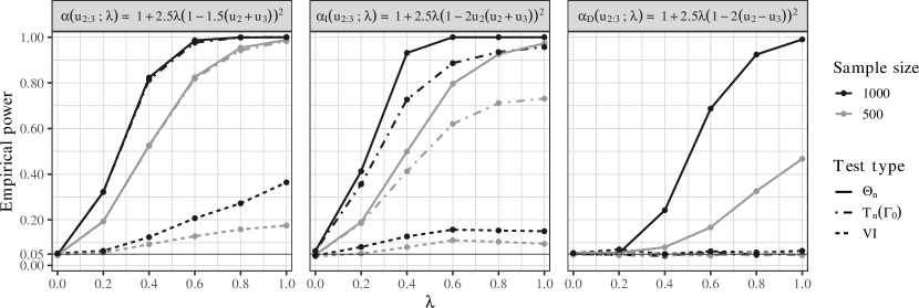
5.1 Power study: The functional form of the conditional copula
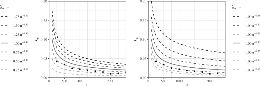
The conditional copula in Example 2 varies in . To alter the variation, we choose values between zero and one for the parameter in the function
| (5.1) |
For , does not vary in . Recall that the simplifying assumption is satisfied in the second tree in Example 2, so that is true if . For , varies in and is false. For the variation is most pronounced. In Figure 6, the variation of the conditional correlation of as a function of the mean is shown on the left hand side.111111 Note that we have already seen for as a function of and as shaded background in the plots on the left hand side of Figure 2 and Figure 5.
For the sample sizes and we apply the CCC test and the VI test [26] for the hypothesis .
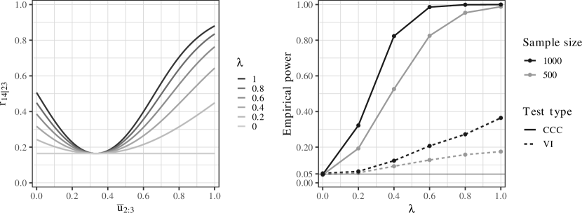
On the right hand side of Figure 6, empirical power values are plotted for different values of the parameter . The numbers are based on samples for each combination of and . The level of the tests is chosen to be 5%. For both tests and sample sizes the empirical size (i.e. the case ) is close to the theoretical level of the test. The empirical power of both tests is clearly increasing for all values of if one doubles the sample size from to observations. Furthermore, both tests are more powerful the more the variation in is pronounced, i.e., the larger the parameter is. In terms of empirical power, the CCC test outperforms the VI test in all settings with a relative improvement that often exceeds 300%. Both tests are implemented in an accompanying R-package pacotest [29] and are computationally feasible. For and a sample size of , the computational time for the CCC test is seconds and for the VI test seconds.121212 The reported computational times are the median from repetitions on a single core of an AMD Ryzen 7 PRO 4750U processor. Note that a major part of the computational time for the CCC test is required for the computation of the asymptotic covariances that account for estimated pseudo-observations from the PPITs. In a fair comparison of computational times, the CCC test can, like the VI test, also be computed with known observations from the PPITs. The computational time of the CCC test then drops to seconds and is much shorter than the seconds of the VI test.
5.2 Power study: Improved power due to the decision tree algorithm
We now compare the CCC test based on the decision tree approach with the CCC test which only considers the base partition . By construction, always holds, meaning that if we reject on the basis of , we also reject on the basis of . As a consequence, the empirical power of is never smaller than the empirical power of . The improvement in power due to the use of instead of depends on the data generating process and will be investigated in the following.
For the base partition we choose as in Section 4. As data generating processes we consider Example 2 and the resulting vine copulas that arise if the parameter of in the edge of tree of Example 2 is given by
| (5.2) | ||||
| or | ||||
| (5.3) | ||||
Figure 7 shows the empirical power of the CCC tests and for the hypothesis . For the case of Example 2 (left panel in Figure 7), the test with the fixed partition delivers a test which performs almost as good as . That is because the parameter of in Example 2 can be written as a function of the mean of the conditioning variables . Furthermore, the conditioning variables are positively associated due to the Clayton copula with . As a result, the decision tree rarely finds a partition which in terms of the test statistic improves over the base partition by an amount larger than the penalty . Therefore, the test statistic often coincides with the test statistic of the base partition.
For the other two cases, the partition is not a good choice and the decision tree algorithm finds substantially better partitions in a data-driven way. The varying parameter of (middle panel in Figure 7) introduces an interaction effect between the two conditioning variables. Although the test with the fixed partition can detect some variation in , the decision tree finds better partitions which can increase the empirical power by more than 20 percentage points. The gain of power is even more pronounced if the parameter of (right panel in Figure 7) is a function of the difference of the conditioning variables. Even if and is strongly varying in , the test with the fixed partition , that is based on the mean of the conditioning variables, cannot recognize the variation. As a result, the empirical power is identical to the level of the test. On the contrary, the data-driven selection of the partition results in a substantial power increase. For and , the power increases from 5% to 99%.
In summary, the choice of the base partition determines a lower bound for the empirical power of the test and the decision tree can increase its power. The magnitude of the improvement depends on the data generating process and ranges from negligible, e.g., , to huge, e.g., . For all data generating processes, the power of the data-driven test is much better than the power of the VI test. The difference is most pronounced for where the empirical power of the VI test is always approximately 5% while the empirical power of the CCC test can be 99%. In Section A.7 we investigate what kind of partitions are typically selected by the decision trees and how they adapt to the different variations in the conditional correlation determined by and .
5.3 Power study: The dimension of the conditioning set
For high-dimensional vine copulas, the dimension of the conditioning set of a conditional copula increases rapidly. Therefore, it is substantial that a test still has power if the dimension of the conditioning set is not small. To investigate the performance of the CCC test w.r.t. the dimension of the conditioning set, we consider a up to twelve-dimensional Clayton copula where the Clayton copula in the edge of the last tree is replaced by a Frank copula with varying parameter.
Example 3
For , the building-blocks of the -dimensional D-vine copula are chosen to be
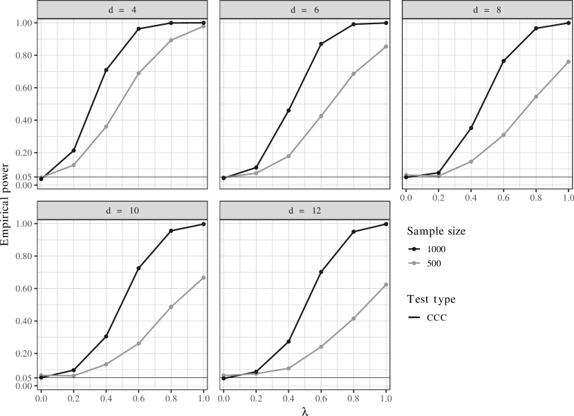
For Example 3 coincides with Example 2 and as before we set and consider different values for . For all dimensions, the functional form of the parameter only depends on the conditioning variables and . Therefore, the variation of in is always the same but the dimension of the testing problem increases with . Grouped by the dimension , the empirical power and size of the VI and the CCC test for the hypothesis are shown in Figure 8.
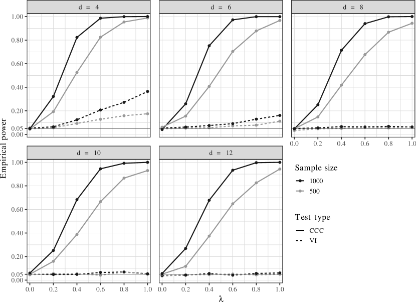
While the empirical power of the VI test decreases a lot if the dimension of the conditioning set is increased, the empirical power of the CCC test decreases only slightly for higher values of . In particular, for the setup and , the power of the VI test drops from 36% to 5% if the dimension is increased from to . On the contrary, the power of the CCC test for this setup is always 100%. Moreover, even when the power of the CCC test is not 100% for , the decrease in its power is still marginal. For instance, for and , the power of the CCC test only decreases from 83% to 67% while the power of the VI test quickly drops to approximately 5% if the dimension is increased from to . Thus, the introduction of a penalty in the CCC test statistic and the data-driven selection of the partition by means of a decision tree yields a test whose power decreases only slightly with the dimension of the conditioning vector.
5.4 Power study: Misspecification of the copulas in the lower trees
The true family of the five copulas in the first and second tree in Example 2 is the Clayton copula. To analyze the effect of misspecified copula families, we now vary the pairwise value of Kendall’s tau between and and estimate either survival Gumbel or Gumbel copulas for all five copulas in the lower trees. The black lines in Figure 9 show the results for correctly specified Clayton copulas in the lower trees as a benchmark. Since the strength of the variation of is more pronounced for higher values of , the empirical power of the tests is also increasing in . The empirical size of the tests () is not influenced by and always close to the theoretical level of 5%.
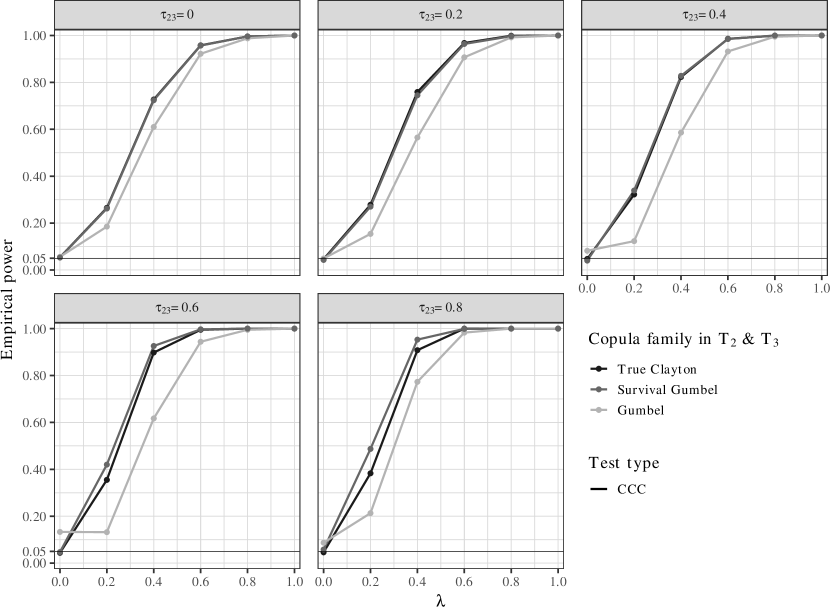
The dark grey line in Figure 9 corresponds to a rather mild misspecification where we estimate survival Gumbel copulas in the first and second tree. We see that the empirical size is still very close to the theoretical level of 5% (). Moreover, the power of the test with misspecified survival Gumbel copulas is almost indistinguishable from the power of the test with correctly specified Clayton copulas. If the degree of misspecification is severe and we fit Gumbel copulas (with upper tail dependence) to data generated from Clayton copulas (with lower tail dependence), differences in the empirical power of the CCC test become visible when comparing the light grey lines with the black lines in Figure 9. In the majority of the considered scenarios the empirical power is now a little smaller. In cases with high dependence, i.e., , the empirical size is increased. This shows that the test might not control the size if the copula families in the lower trees are severely misspecified. Note that we misspecify five copula families and that the misspecification in the second tree might be even worse because the data in the edges of the second tree is no longer generated by Clayton copulas if the copulas in the first tree are misspecified. Thus, the performance of the CCC test appears to be relatively robust w.r.t. such a severe misspecification.
6 A hierarchical procedure for testing the simplifying assumption in vine copulas
Up to now, we have tested single building blocks of vine copulas, i.e., the hypothesis for a fixed edge . To check the simplifying assumption for a -dimensional R-vine copula with fixed structure , one has to check this constraint for edges. In order to control the family-wise error rate , we apply the Bonferroni correction and test the set of hypotheses131313 For each hypothesis corresponding to a fixed edge we use the same CCC test settings as before, i.e., decision trees with depth , for the penalty and (see equation (4.1)) as base partition.
We use a hierarchical procedure and begin with testing the hypotheses in the second tree. We then only check the hypotheses for the next tree if the validity of the simplifying assumption could not be rejected for tree , for . The hierarchical procedure is stopped whenever an individual hypothesis is rejected at a level of . As a result, the hierarchical procedure detects critical building blocks of a vine copula model where a pair-copula does not seem to be an adequate model for the bivariate conditional copula of the bivariate conditional distribution . The procedure is also in line with the common sequential specification and estimation of simplified vine copulas and can be integrated in model selection algorithms as demonstrated in Kraus and Czado [27].
6.1 Simulation study
In the following simulation study we test the simplifying assumption for the four-dimensional Clayton, Gaussian, Gumbel, and Frank copula with pair-wise values of Kendall’s of . Since each copula is exchangeable an arbitrary structure can be fixed. We fit a D-vine copula and select the copula families of , , , , , using the AIC. The hierarchical procedure is applied to test the simplifying assumption at a theoretical level of 5%. Thus, in tree two conditional copulas are tested with an individual level of 1.67%. If we do not reject the for both copulas in tree , we continue in tree and test at an individual level of 1.67%.
The two upper panels in Figure 10 report the results for the four-dimensional Clayton and Gaussian copula for which the simplifying assumption is satisfied [44].

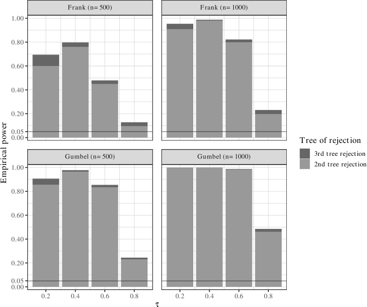
The empirical size of the hierarchical test procedure with the CCC test is close to the theoretical level even under consideration of possibly misspecified copula families. In the lower panels of Figure 10, the empirical power for the four-dimensional Frank and Gumbel copula is plotted. The Frank and Gumbel copula violate the simplifying assumption as long as [44]. Although the variation in the conditional copulas induced by the four-dimensional Frank and Gumbel copulas is rather mild (see Figure 11), the CCC test often rejects the simplifying assumption.
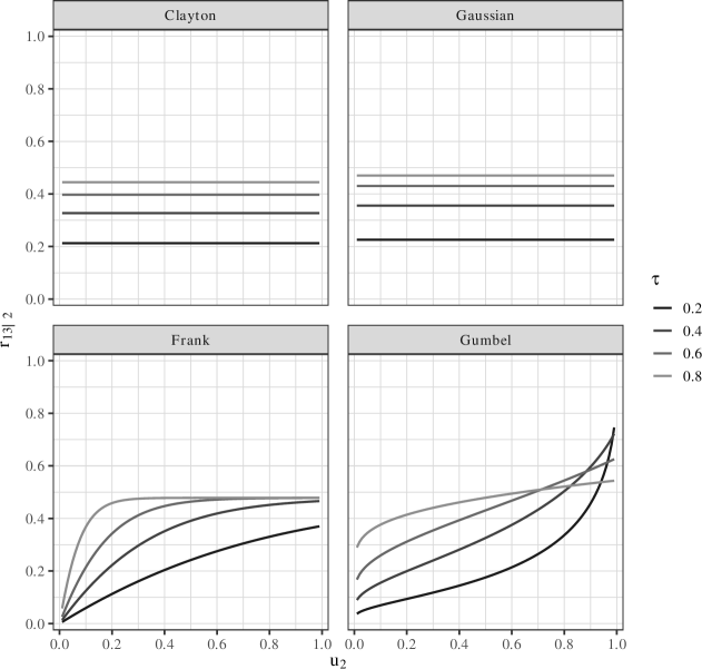
That the power has a minimum at can be explained by the fact that both copulas satisfy the simplifying assumption for and the variation of the conditional correlations (see Figure 11) is less pronounced than for .
How the decision trees adapt to the variation of the conditional correlations can be seen by looking at the most frequently selected decision trees and the resulting partitions. For the Frank copula (with and ) the most frequently selected decision tree in tree of the vine (selected in 21.28% of all simulated cases) consists of a first split according to the 25% quartile and a second split at the 50% quartile in the left part and at the 25% quartile in the right part, i.e.,
Thus, the partition is most granular for smaller values of the conditioning variable. This is also the area where the variation of the Frank copula is most pronounced as can be seen from Figure 11. In contrast, for the Gumbel copula (with and ) the most common selected partition in tree (selected in 18.51% of all simulated cases) is
Comparing with Figure 11, which shows the conditional correlation for the Gumbel copula, we see that the decision tree adapts to the variation of the conditional correlation by selecting the most granular splits for higher values of the conditioning variable.
Two hypotheses are tested in tree and, provided there is no rejection in tree , one additional hypothesis is tested in tree when the hierarchical procedure for testing the simplifying assumption is applied to four-dimensional vine copulas. In the simulation study, most of the rejections for the four-dimensional Frank and Gumbel copula happen in tree . In Figure 12 we decompose the empirical power of the hierarchical procedure with the CCC test into second tree and third tree rejections. Over all considered scenarios 94.09% and 98.06% of the rejections occur in the second tree for the Frank and Gumbel copula, respectively.
Finally, we revisit the up to twelve-dimensional Example 3 from Appendix 5.3. In Appendix 5.3 we only tested one hypothesis in the last tree and analyzed the effect of an increasing dimensionality of the conditioning set on the empirical power of the CCC test. Now we apply the hierarchical procedure to test the simplifying assumption for the entire D-vine copula with fixed structure defined in Example 3 for and test the set of hypotheses
As mentioned before, the simplifying assumption for a -dimensional vine copula is equivalent to hypotheses. This means that for Example 3 we might test hypotheses for but only the last hypothesis actually violates the simplifying assumption for .
The empirical size and power of the hierarchical procedure with the CCC test to test the simplifying assumption for data generated from Example 3 is shown in Figure 13.
For the simplifying assumption is satisfied and the empirical size is close to the theoretical level of 5%. Similar to Appendix 5.3, we observe that the empirical power of the hierarchical procedure with the CCC test is slightly decreasing in the dimension . The effect is more pronounced for the smaller sample size as compared to . Note that for only one of 55 building blocks of the vine copula violates the simplifying assumption. This explains why for and the empirical power of 62% is lower than the empirical power of 94% when only the last building block is tested (see Figure 8). However, a sample size of is sufficiently large so that the empirical power of the hierarchical procedure with the CCC test is still almost 100% in this scenario.
6.2 Real data applications
We now use the hierarchical procedure with the CCC test to test the simplifying assumption for R-vine copulas fitted to four different real data sets. The dimensionality of the data varies between and and the number of observations between and . On the one hand, we consider the data set uranium [9] and obtain normalized ranks as pseudo-observations from the copula by means of the rescaled ecdf. On the other hand, we consider three financial data sets from the Kenneth R. French – Data Library (available under: http://mba.tuck.dartmouth.edu/pages/faculty/ken.french/data_library.html). We apply ARMA(,)-GARCH(,)-filtering [12, 6] with t-distributed innovations and apply the rescaled ecdf to the residuals to obtain pseudo-observations from the copulas.141414Copula modeling for GARCH-filtered return data has been studied in [8, 7] and [38] provides a review of copula models for economic time series.
In order to test the simplifying assumption with the CCC test, the researcher has to specify the vine structure , which also determines the , and the copula families for the edges. The selection of the vine structure and copula families is commonly based on the data, e.g., by using the algorithm of Dißmann et al. [11]. If model selection and statistical inference is done on the same data, statistical inference might no longer be valid (see Fithian, Sun and Taylor [13] or Lee et al. [31] for a discussion of post model selection inference). Therefore, we randomly split the samples into two parts so that the partial vine copula model is selected on one half of the data and the other half of the data is used to apply the CCC test. To obtain parametric models for the PVC we apply the standard R-vine model selection algorithm proposed by Dißmann et al. [11] which is implemented in the R-package VineCopula [35]. The resulting vine structure and copula families are then used to fit a model for the partial vine copula and conduct tests on the other half of the data.
In Table 2 we provide information about all four data sets and report the results of the hierarchical test procedure with the CCC test .151515Note that the CCC test is not a consistent test because the conditional correlation can be constant if the simplifying assumption is false. Moreover, if the conditional correlation is varying it may be possible that this variation is not detected by the proposed CCC test with the decision tree based partitioning as described in Section 4.2. For all cases where the validity of the simplifying assumption is rejected, we show the first tree in which we reject at least one null hypothesis of the form and stop the hierarchical test procedure. Moreover, the smallest p-value of one hypothesis of the hierarchical procedure is also depicted.
| Name | uranium | FF3F | FF5F | Ind10 |
| Description | Uranium Exploration Data Set | Fama/French 3 Factors | Fama/French 5 Factors | 10 Industry Portfolios |
| Source | Cook and Johnson [9], R-package copula | Kenneth R. French – Data Library | Kenneth R. French – Data Library | Kenneth R. French – Data Library |
| Variables | log concentration of Uranium, Lithium, Cobalt, Potassium, Cesium, Scandium, Titanium | SMB, HML, | SMB, HML, RMW, CMA, | 10 industry portfolios formed according to four-digit SIC codes. |
| Period | — |
02-Jan-2001 to
31-Dec-2020 (daily) |
02-Jan-2001 to
31-Dec-2020 (daily) |
02-Jan-2001 to
31-Dec-2020 (daily) |
| Dimension |
7
(21 pair-copulas) |
3
(3 pair-copulas) |
5
(10 pair-copulas) |
10
(45 pair-copulas) |
| Test decision of the hierarchical procedure (at a 5% significance level) | The simplifying assumption can be rejected in tree . | The simplifying assumption cannot be rejected. | The simplifying assumption cannot be rejected. | The simplifying assumption cannot be rejected. |
| Smallest p-value [Bonferroni adjusted p-value] of one hypothesis of the hierarchical procedure |
[] |
[] |
[] |
[] |
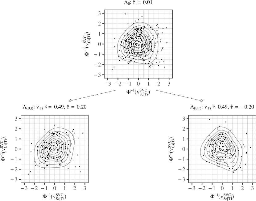
For the non-financial data example uranium we reject the simplifying assumption already in tree . The rejection is in line with the results reported by Gijbels, Omelka and Veraverbeke [17] and Kraus and Czado [27]. In Figure 14 we provide a visualization of the rejected building block for the uranium data set. The grouped scatterplots are formed according to the decision tree used for the CCC test . For easier visual inspection the margins are transformed to be standard normal and contours derived from copula kernel density estimates (R-package kdecopula [33]) are shown. The plots show that the conditional copula of Scandium (Sc) and Cesium (Cs) given Titanium (Ti) is varying with an estimated positive correlation of for values of Titanium being smaller than its median and a negative estimated correlation of for larger values of Titanium.
For the three filtered financial returns the simplifying assumption cannot be rejected on the basis of the CCC test (Table 2). This indicates that the possible violation of the simplifying assumption for the vine copulas selected by Dißmann’s algorithm might be less severe for this kind of data as compared to uranium. This is consistent with the findings of Kraus and Czado [27] who also use the CCC test and report that the simplifying assumption seems to be rather appropriate for filtered financial returns.
7 Conclusion
In practical applications, a test for the simplifying assumption in high-dimensional vine copulas must be computationally feasible and tackle the curse of dimensionality. The introduced hierarchical procedure with the CCC test addresses these two issues.
The asymptotic distribution of the CCC test statistic is derived under the assumption of semi-parametrically estimated pseudo-observations from the partial probability integral transforms. Since the test has a known asymptotic distribution and is based on the stepwise maximum likelihood estimator, it is computationally feasible also in high dimensions. To prevent suffering from the curse of dimensionality, the CCC test utilizes a novel stochastic interpretation of the simplifying assumption based on the partial vine copula. Moreover, we propose a discretization of the support of the conditioning vector into a finite number of subsets and incorporate a penalty in the test statistic. A decision tree algorithm looks for the largest deviation from the simplifying assumption measured in terms of conditional correlations and also contributes to a computationally feasible test.
In a simulation study we provide a thorough analysis of the finite sample performance of the CCC test for various kinds of data generating processes. The CCC test outperforms the vectorial independence test by a large margin if the conditional correlation is varying. Even more important for high-dimensional applications, the simulation study demonstrates that the power of the test decreases only slightly with the dimension of the conditioning vector. A moderate misspecification of the parametric copula families does not affect the power properties of the CCC test. We also investigate the performance of a hierarchical procedure that utilizes the CCC test to test the simplifying assumption. An application to four real data sets demonstrates the usefulness of the test and indicates that the validity of the simplifying assumption should be checked individually for each data set.
The CCC test can also be utilized to improve the modeling of data with vine copulas. Schellhase and Spanhel [40] make use of the CCC test to identify building blocks of vine copulas where the simplifying assumption does not seem to be adequate and the estimation of a conditional copula that is varying in its conditioning variables can improve the modeling. Additionally, Kraus and Czado [27] use the CCC test to find alternative vine copula structures which might be more in line with the simplifying assumption.
Appendix
A.1 Proof of 1
That (i) and (ii) are equivalent follows from the definition of the simplifying assumption in 1 and the definition of the conditional and partial copula in Definition 1.
For , implies by Lemma 3.1 in Spanhel and Kurz [43]. Thus, and are equal in distribution and . This shows (ii) (iii).
To show (ii) (iii), we use induction over the trees. By the definition of the PPITs in the second tree we have that
Because (ii) implies that
it follows that
and the base case of the induction is proved.
We now assume the induction hypothesis that for tree
holds. Note that Lemma 3.1 in Spanhel and Kurz [43] then implies that
| (A.1) |
By (ii), we get for each in tree and that
| (A.2) | ||||
where and are chosen such that .161616 By the proximity condition of the R-vine (Definition 2) there exists a such that either or with and w.l.o.g. we use the first case in (A.2). Note that is the distribution of and the distribution of . By (A.1) it follows that . Thus,
| (A.3) | ||||
| (A.4) |
where (A.3) follows from (A.1) and (A.4) is the definition of . As a result, we have shown that
Finally, (ii) implies that
A.2 Proof of Proposition 2
We first prove the following lemma stating the asymptotic distribution of the test statistic under and the assumption that observations from the PPITs are observable.
Lemma 1
Let be independent copies of and . Consider a fixed R-vine structure and let be a fixed edge. Assume that the partition satisfies the conditions stated in Proposition 2. Under it holds that
Proof.
We first derive the asymptotic distribution of under before showing that has an asymptotic chi-square distribution under . For this purpose, let , denote the Kronecker product, be a column vector of ones and be the identity matrix, so that is a matrix that can be used to extract every fifth element from a -dimensional column vector. The correlations are then given by , with being the unique solution of the estimating equation
| (A.5) |
where the estimating function will be stated in the following.
Define
where . The solution of denotes the random fraction of data corresponding to , i.e.,
Define
where . For we set
The estimating function in (A.5) is given by
Let be the unique solution of , be the unique solution of , and so that for all under because for each -th block element of it holds that
Using the same steps it can be readily verified that for all under . Thus, under , the standard theory of estimating equations for two-step estimators, e.g., Theorem 6.1 in Newey and McFadden [36], yields that
| (A.6) |
where , and denotes a -dimensional normal distribution with mean vector and covariance matrix .
If we now extract every fifth element from using , we obtain the joint asymptotic distribution of the estimated correlations under as
so that
Under it holds that and therefore it follows with the first-order difference matrix and the continuous mapping theorem, that
To obtain the statistic of the CCC test when a sample from the PPITs is observable, the covariance matrix
has to be consistently estimated, e.g., by , where denotes the sample covariance of the random vector . By applying once more the continuous mapping theorem and Slutsky’s theorem, we get
and Lemma 1 is proven.
The remaining part of the proof of Proposition 2 requires the definition of the pseudo stepwise maximum likelihood estimator of the vine copula parameters. This estimator can be obtained as the solution of estimating equations (Hobæk Haff [20], Spanhel and Kurz [42], Tsukahara [46]). By extending these estimating equations by the ones for the correlations defined in the proof of Lemma 1 we derive the asymptotic distribution of the CCC test when pseudo-observations from the PPITs are estimated. Consider a fixed R-vine structure and let be a parametric simplified vine copula such that so that , where denotes the PVC of . The density of is given by
where is a bivariate copula for each with parameter . For , the vector collects the parameters in tree and the vector collects all parameters up to and including tree . The individual stepwise pseudo score functions for the copulas in tree are given by
. Here, the pseudo-observations of the PPITs for , are defined by
and for as
| (A.7) |
where and is selected as in 3.
Set and define the estimating function
so that the solution of is the pseudo stepwise maximum likelihood estimator.
Moreover, denotes the estimating function of the correlations when pseudo-observations from the PPITs are used, i.e.,
where
Let so that the estimating function of the vine copula parameters and the correlations is given by
The rank approximate estimator is then given as the solution of where is given as in the proof of Lemma 1. To derive the asymptotic distribution of , introduce
where is the unique solution of for all under . By the same reasoning as in the proof of Lemma 1 and because does not depend on it follows that for all under . Thus, provided the regularity conditions in Theorem 1 in Hobæk Haff [20] are satisfied, it follows that
where with and is the number of vine copula parameters, i.e., the length of the vector .
To extract the estimated correlations from and to obtain the corresponding asymptotic covariance matrix, we can exploit the block-structure of as follows
Denote the matrix consisting of zeros by and define so that . The asymptotic covariance matrix of is then
Thus, under it follows that
With the same arguments as in the proof of Lemma 1 this implies under
where
| (A.8) |
is a consistent estimator of .171717 See Genest, Ghoudi and Rivest [15] for a consistent estimator of .
A.3 Proof of Proposition 3
To obtain the asymptotic distribution of the test statistic , we need the following lemmas.
Lemma 2
Let , where is the cdf of a continuous probability distribution. Additionally, let be a penalty function satisfying the conditions stated in Proposition 3. If it holds that , i.e.,
Proof.
Let . Since it holds that
| (A.9) |
By assumption converges in distribution to , therefore
| (A.10) |
Moreover, . Thus, it holds that
Thus,
In the following Lemma 3 the asymptotic behavior of is analyzed.
Lemma 3
Let be sequences of
random variables and
, , random variables with continuous cumulative distribution functions.
Further let be a penalty function satisfying the conditions stated in Proposition 3.
Define .
-
(i)
If for each , it holds that .
-
(ii)
If there is an such that then .
Proof.
Proof of (i). Let , then
Using the Fréchet-Hoeffding inequalities [14, 22] we have
| and | ||||
Due to the continuity of the minimum and maximum as well as Lemma 2 it follows that
| and | ||||
| (A.11) | ||||
Thus,
Proof of (ii). For , define . Because it follows that . Note that for all because .
Thus, the Fréchet-Hoeffding upper bound implies that for any ,
and the proof is complete.
Using Proposition 2 and setting in Lemma 3 (i) it follows that the statistic converges under to a distribution.
A.4 The decision tree: Algorithmic details
Every leaf in the decision tree represents a subset of the support of the random vector . The maximum depth of the decision tree is denoted by and every leaf is assigned to a level in the decision tree (). The level of a leaf refers to the number of splits which have already been used to arrive at the leaf, starting from the root leaf (see Figure 15).
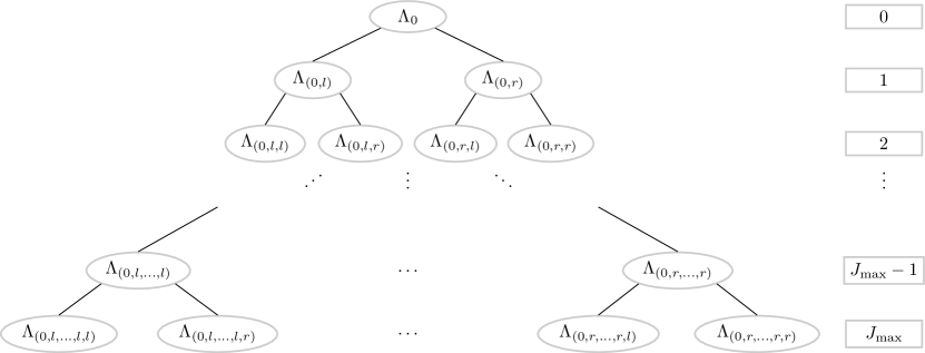
A leaf is denoted by , where the -dimensional vector is the unique identifier for a leaf in the -th level of the decision tree. That is, the two leaves in the -th level of the decision tree being connected via edges to the leaf in the -th level are identified by with . The subsets assigned to the leafs in the -th level by a binary split are given by
Every split is chosen out of a finite number of possible splits. A possible split in the leaf is defined as a pair of disjoint subsets of , i.e., with . From these possible splits, the split is selected that maximizes the statistic of the CCC test. Meaning that every split is defined as
Thus, the subsets that are transferred to leaf , , after using the optimal split , are given by and . In the last level we obtain a final partition of the support into disjoint subsets given by . For the final partition we compute the value of the test statistic
In all simulations in Section 5 and the real data applications in Section 6.2, we choose for the penalty and as base partition.181818The partition is defined in equation (4.1) in Section 4.1. Further tuning parameters of the decision tree are the maximum depth of the tree and the set of possible splits . To keep the test computationally feasible and because it performs well in simulations, we consider a maximum depth of and the number of possible splits in each leaf is restricted to be at most in tree . The considered splits are as follows: To obtain the sets and for the two leaves in level 1, we consider the empirical 25%, 50% and 75% quartiles for each conditioning variable , . If , we additionally take the empirical 25%, 50% and 75% quartiles of the mean aggregated conditioning variables into account, resulting in possible splits. A formal definition of the set of possible splits is given in Appendix A.5. The sets and for the four leaves in level 2 are obtained in the same fashion except that we now condition on or , respectively. Furthermore, we use several restrictions in the decision tree algorithm to guarantee that the final data sets do not become too small.191919 A decision tree with two or three splits is only applied if we have a certain amount of data. This is implemented by introducing a tuning parameter which controls the minimum sample size per leaf in the decision tree (the default value is 100 observations). As a result we do not always use the 25%, 50% and 75% quartiles as thresholds but depending on the available sample size we may only use the 50% quartile or even don’t apply any additional split at all.
A.5 Formal definition of the set of possible splits for the decision tree
If denotes the empirical -quantile of the vector , the set of possible splits in the leaf , for and , with -dimensional conditioning set is given by
with
and . We further used the notation for and the index set is defined as .
A.6 Choosing the penalty function: A finite sample analysis
To apply the test based on the statistic , a penalty function has to be specified and any choice satisfying the conditions stated in Proposition 3 results in an asymptotically valid test. However, the size and power for finite sample sizes depends on the chosen penalty function . In the following, the choice of the penalty function in finite samples will be analyzed in a simulation study under , i.e., with a focus on the empirical size.
In all simulations in Section 5 and the real data applications in Section 6.2, we choose for the penalty and as base partition.202020The partition is defined in equation (4.1) in Section 4.1. As mentioned in Section 5.2, the test statistic (the CCC test with fixed partition ) is related to the test statistic (the CCC test with a decision tree selected partition) in the following way. For , with , it holds
meaning that if we reject based on , we also reject based on . It follows that the empirical size of is bounded from below by the empirical size of when both tests are applied to the same collection of data sets in a monte carlo simulation to compute the empirical size.
We now derive a condition on such that and result in equivalent test decisions. This means that the test statistic is analyzed relative to .212121 An extensive simulation study of the finite sample performance of the proposed test is presented in Section 5 where the empirical size relative to the theoretical level of the test is studied. Let , where is the cardinality of , i.e., the number of subsets forming the partition . If the penalty function satisfies
| (A.12) |
it follows that . Therefore, if we cannot reject at a -level based on and if satisfies (A.12), we also cannot reject based on , i.e., if it holds
As a result, if , both tests result in the same -level test decisions, i.e.,
Note that converges in distribution to a -distribution under and by Slutsky’s theorem it follows that . Therefore, the lower bound is bounded in probability, i.e.,
Meaning that for any , we can choose such that , which restricts the probability of different test decisions (i.e., rejecting the with but not rejecting the with ) at a -level to because
This implies that for any , we can choose such that and therefore
In practical applications, we are interested in the finite sample distribution of the lower bound of the penalty function . Using resampling techniques, we can determine this lower bound for under .
To illustrate how one can use resampling techniques to determine the parameters and of the penalty function , we again consider the data generating process given in Example 2. For , the null hypothesis is true. For each considered sample size we generate random samples of size from the four-dimensional D-vine copula and compute for each sample the lower bound of the penalty function . In Figure 16, the maximum of all lower bounds in the different samples is plotted for different sample sizes as dots. By taking the maximum over all resampled lower bounds we identify a lower bound for the penalty which would guarantee that in every of the samples the asymptotic -level test decisions are the same, i.e., . The level of the test is chosen to be 5% and the lines correspond to different choices of the penalty function . The level of the penalty function is varied for a fixed power of in the plot on the left hand side of Figure 16 and the power of the penalty function is varied for a fixed level of on the right hand side. The solid line corresponds to the penalty function which we use in all the simulations and applications. One can see that the choice of the penalty function is reasonable in comparison to the lower bounds obtained via resampling techniques for all sample sizes between and observations, as the penalty is for all sample sizes considerably larger than the lower bounds.
A.7 An analysis of the typical partitions selected by the decision trees
The following analysis complements the simulation study in Section 5.2 by an analysis of the partitions typically selected by the decision trees. To investigate what kind of partitions are selected by the decision trees and how they adapt to the different variations in the conditional correlation determined by and (see (5.1), (5.2) and (5.3)), we focus on the case and a sample size of . If the variation of the copula parameter is given by , the first split is most often done with respect to the 75% quartile of (in 93.6% of the simulated samples). The most frequently selected partition (in 40.6% of the samples) consists of two more splits with respect to the quartiles of in the next level. This partition is visualized in the left panel of Figure 17.
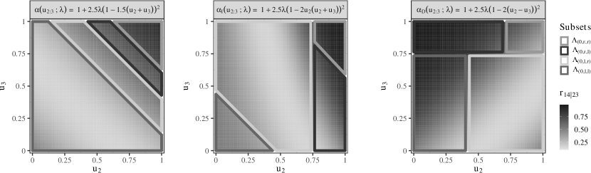
The adaption of the decision tree based partition to the variation in the conditional correlation becomes evident when looking at the shaded background which shows the conditional correlation of as a function of and .
The middle panel in Figure 17 shows the most frequently selected partition (in 14.8% of the samples) if the variation of the copula parameter is given by which contains an interaction effect between the two conditioning variables. In this case, the first split is most often done with respect to the 75% quartile of (in 61.7% of the samples). The decision tree adapts to this variation in the conditional correlation, shown as shaded background, by choosing splits with respect to the quartiles of in the second level.
The right panel in Figure 17 visualizes the most frequently selected partition (in 22.7% of the samples) if the variation of the copula parameter is given by . Here, the two conditioning variables have an opposite sign in the definition of . In this case, the first split is most often done with respect to the 75% quartile of (in 52.8% of the samples). Once again, the decision tree adapts to the variation in the conditional correlation, shown as shaded background, by choosing splits with respect to the quartiles of the other variable in the second level.
[Acknowledgments] We are very grateful for the helpful comments of two anonymous reviewers, an associate editor and the editor. Malte S. Kurz acknowledges funding by the Deutsche Forschungsgemeinschaft (DFG, German Research Foundation) – Project Number 431701914.
References
- Aas et al. [2009] {barticle}[author] \bauthor\bsnmAas, \bfnmK.\binitsK., \bauthor\bsnmCzado, \bfnmC.\binitsC., \bauthor\bsnmFrigessi, \bfnmA.\binitsA. and \bauthor\bsnmBakken, \bfnmH.\binitsH. (\byear2009). \btitlePair-copula constructions of multiple dependence. \bjournalInsurance: Mathematics and Economics \bvolume44 \bpages182–198. \endbibitem
- Acar, Craiu and Yao [2013] {barticle}[author] \bauthor\bsnmAcar, \bfnmE. F.\binitsE. F., \bauthor\bsnmCraiu, \bfnmR. V.\binitsR. V. and \bauthor\bsnmYao, \bfnmF.\binitsF. (\byear2013). \btitleStatistical testing of covariate effects in conditional copula models. \bjournalElectronic Journal of Statistics \bvolume7 \bpages2822–2850. \endbibitem
- Bedford and Cooke [2001] {barticle}[author] \bauthor\bsnmBedford, \bfnmT.\binitsT. and \bauthor\bsnmCooke, \bfnmR. M.\binitsR. M. (\byear2001). \btitleProbability density decomposition for conditionally dependent random variables modeled by vines. \bjournalAnnals of Mathematics and Artificial Intelligence \bvolume32 \bpages245–268. \endbibitem
- Bedford and Cooke [2002] {barticle}[author] \bauthor\bsnmBedford, \bfnmT.\binitsT. and \bauthor\bsnmCooke, \bfnmR. M.\binitsR. M. (\byear2002). \btitleVines – A new graphical model for dependent random variables. \bjournalThe Annals of Statistics \bvolume30 \bpages1031–1068. \endbibitem
- Bergsma [2004] {bunpublished}[author] \bauthor\bsnmBergsma, \bfnmW. P.\binitsW. P. (\byear2004). \btitleTesting conditional independence for continuous random variables. \bnoteURL: https://www.eurandom.tue.nl/reports/2004/048-report.pdf. \endbibitem
- Bollerslev [1986] {barticle}[author] \bauthor\bsnmBollerslev, \bfnmTim\binitsT. (\byear1986). \btitleGeneralized autoregressive conditional heteroskedasticity. \bjournalJournal of Econometrics \bvolume31 \bpages307–327. \endbibitem
- Chan et al. [2009] {barticle}[author] \bauthor\bsnmChan, \bfnmNgai-Hang\binitsN.-H., \bauthor\bsnmChen, \bfnmJian\binitsJ., \bauthor\bsnmChen, \bfnmXiaohong\binitsX., \bauthor\bsnmFan, \bfnmYanqin\binitsY. and \bauthor\bsnmPeng, \bfnmLiang\binitsL. (\byear2009). \btitleStatistical Inference for Multivariate Residual Copula of GARCH Models. \bjournalStatistica Sinica \bvolume19 \bpages53–70. \endbibitem
- Chen and Fan [2006] {barticle}[author] \bauthor\bsnmChen, \bfnmXiaohong\binitsX. and \bauthor\bsnmFan, \bfnmYanqin\binitsY. (\byear2006). \btitleEstimation of copula-based semiparametric time series models. \bjournalJournal of Econometrics \bvolume130 \bpages307–335. \endbibitem
- Cook and Johnson [1986] {barticle}[author] \bauthor\bsnmCook, \bfnmR. Dennis\binitsR. D. and \bauthor\bsnmJohnson, \bfnmMark E.\binitsM. E. (\byear1986). \btitleGeneralized Burr-Pareto-Logistic Distributions With Applications to a Uranium Exploration Data Set. \bjournalTechnometrics \bvolume28 \bpages123–131. \endbibitem
- Derumigny and Fermanian [2017] {barticle}[author] \bauthor\bsnmDerumigny, \bfnmA.\binitsA. and \bauthor\bsnmFermanian, \bfnmJ. D.\binitsJ. D. (\byear2017). \btitleAbout tests of the “simplifying” assumption for conditional copulas. \bjournalDependence Modeling \bvolume5 \bpages154–197. \endbibitem
- Dißmann et al. [2013] {barticle}[author] \bauthor\bsnmDißmann, \bfnmJ.\binitsJ., \bauthor\bsnmBrechmann, \bfnmE. C.\binitsE. C., \bauthor\bsnmCzado, \bfnmC.\binitsC. and \bauthor\bsnmKurowicka, \bfnmD.\binitsD. (\byear2013). \btitleSelecting and estimating regular vine copulae and application to financial returns. \bjournalComputational Statistics & Data Analysis \bvolume59 \bpages52–69. \endbibitem
- Engle [1982] {barticle}[author] \bauthor\bsnmEngle, \bfnmRobert F.\binitsR. F. (\byear1982). \btitleAutoregressive Conditional Heteroscedasticity with Estimates of the Variance of United Kingdom Inflation. \bjournalEconometrica \bvolume50 \bpages987–1007. \endbibitem
- Fithian, Sun and Taylor [2014] {bunpublished}[author] \bauthor\bsnmFithian, \bfnmWilliam\binitsW., \bauthor\bsnmSun, \bfnmDennis\binitsD. and \bauthor\bsnmTaylor, \bfnmJonathan\binitsJ. (\byear2014). \btitleOptimal Inference After Model Selection. \bnoteArXiv e-prints arXiv:1410.2597. \endbibitem
- Fréchet [1951] {barticle}[author] \bauthor\bsnmFréchet, \bfnmM.\binitsM. (\byear1951). \btitleSur les tableaux de corrélation dont les marges sont données. \bjournalAnnales de l’Université de Lyon, Section A, Series 3 \bvolume14 \bpages53–77. \endbibitem
- Genest, Ghoudi and Rivest [1995] {barticle}[author] \bauthor\bsnmGenest, \bfnmC.\binitsC., \bauthor\bsnmGhoudi, \bfnmK.\binitsK. and \bauthor\bsnmRivest, \bfnmL. P.\binitsL. P. (\byear1995). \btitleA semiparametric estimation procedure of dependence parameters in multivariate families of distributions. \bjournalBiometrika \bvolume82 \bpages543–552. \endbibitem
- Gijbels, Omelka and Veraverbeke [2015] {barticle}[author] \bauthor\bsnmGijbels, \bfnmIrène\binitsI., \bauthor\bsnmOmelka, \bfnmMarek\binitsM. and \bauthor\bsnmVeraverbeke, \bfnmNoël\binitsN. (\byear2015). \btitlePartial and average copulas and association measures. \bjournalElectronic Journal of Statistics \bvolume9 \bpages2420–2474. \endbibitem
- Gijbels, Omelka and Veraverbeke [2017] {barticle}[author] \bauthor\bsnmGijbels, \bfnmIrène\binitsI., \bauthor\bsnmOmelka, \bfnmMarek\binitsM. and \bauthor\bsnmVeraverbeke, \bfnmNoël\binitsN. (\byear2017). \btitleNonparametric testing for no covariate effects in conditional copulas. \bjournalStatistics \bvolume51 \bpages475–509. \endbibitem
- Gijbels et al. [2017] {barticle}[author] \bauthor\bsnmGijbels, \bfnmIrène\binitsI., \bauthor\bsnmOmelka, \bfnmMarek\binitsM., \bauthor\bsnmPešta, \bfnmMichal\binitsM. and \bauthor\bsnmVeraverbeke, \bfnmNoël\binitsN. (\byear2017). \btitleScore tests for covariate effects in conditional copulas. \bjournalJournal of Multivariate Analysis \bvolume159 \bpages111–133. \endbibitem
- Grothe and Nicklas [2013] {barticle}[author] \bauthor\bsnmGrothe, \bfnmOliver\binitsO. and \bauthor\bsnmNicklas, \bfnmStephan\binitsS. (\byear2013). \btitleVine constructions of Lévy copulas. \bjournalJournal of Multivariate Analysis \bvolume119 \bpages1–15. \endbibitem
- Hobæk Haff [2013] {barticle}[author] \bauthor\bsnmHobæk Haff, \bfnmI.\binitsI. (\byear2013). \btitleParameter estimation for pair-copula constructions. \bjournalBernoulli \bvolume19 \bpages462–491. \endbibitem
- Hobæk Haff, Aas and Frigessi [2010] {barticle}[author] \bauthor\bsnmHobæk Haff, \bfnmI.\binitsI., \bauthor\bsnmAas, \bfnmK.\binitsK. and \bauthor\bsnmFrigessi, \bfnmA.\binitsA. (\byear2010). \btitleOn the simplified pair-copula construction – Simply useful or too simplistic? \bjournalJournal of Multivariate Analysis \bvolume101 \bpages1296–1310. \endbibitem
- Hoeffding [1940] {bbook}[author] \bauthor\bsnmHoeffding, \bfnmW.\binitsW. (\byear1940). \btitleMaßtabinvariante Korrelationstheorie. \bseriesSchriften des Mathematischen Instituts und des Instituts für Angewandte Mathematik an der Universität Berlin, 5. \endbibitem
- Joe [1996] {bincollection}[author] \bauthor\bsnmJoe, \bfnmH.\binitsH. (\byear1996). \btitleFamilies of -Variate Distributions With Given Margins and Bivariate Dependence Parameters. In \bbooktitleDistributions with Fixed Marginals and Related Topics, IMS Lecture Notes – Monograph Series (\beditor\bfnmL.\binitsL. \bsnmRüschendorf, \beditor\bfnmB.\binitsB. \bsnmSchweizer and \beditor\bfnmM. D.\binitsM. D. \bsnmTaylor, eds.) \bpages120–141. \endbibitem
- Joe [1997] {bbook}[author] \bauthor\bsnmJoe, \bfnmHarry\binitsH. (\byear1997). \btitleMultivariate Models and Dependence Concepts. \bpublisherChapman & Hall, \baddressLondon. \endbibitem
- Joe, Li and Nikoloulopoulos [2010] {barticle}[author] \bauthor\bsnmJoe, \bfnmHarry\binitsH., \bauthor\bsnmLi, \bfnmHaijun\binitsH. and \bauthor\bsnmNikoloulopoulos, \bfnmAristidis K.\binitsA. K. (\byear2010). \btitleTail dependence functions and vine copulas. \bjournalJournal of Multivariate Analysis \bvolume101 \bpages252–270. \endbibitem
- Kojadinovic and Holmes [2009] {barticle}[author] \bauthor\bsnmKojadinovic, \bfnmI.\binitsI. and \bauthor\bsnmHolmes, \bfnmM.\binitsM. (\byear2009). \btitleTests of independence among continuous random vectors based on Cramér-von Mises functionals of the empirical copula process. \bjournalJournal of Multivariate Analysis \bvolume100 \bpages1137–1154. \endbibitem
- Kraus and Czado [2017] {bunpublished}[author] \bauthor\bsnmKraus, \bfnmD.\binitsD. and \bauthor\bsnmCzado, \bfnmC.\binitsC. (\byear2017). \btitleGrowing simplified vine copula trees: improving Dißmann’s algorithm. \bnoteArXiv e-prints arXiv:1703.05203. \endbibitem
- Kurowicka and Joe [2011] {bbook}[author] \beditor\bsnmKurowicka, \bfnmDorota\binitsD. and \beditor\bsnmJoe, \bfnmHarry\binitsH., eds. (\byear2011). \btitleDependence Modeling. \bpublisherWorld Scientific, \baddressSingapore. \endbibitem
- Kurz [2021] {bmanual}[author] \bauthor\bsnmKurz, \bfnmMalte S.\binitsM. S. (\byear2021). \btitlepacotest: Testing for Partial Copulas and the Simplifying Assumption in Vine Copulas \bnoteURL: https://CRAN.R-project.org/package=pacotest, R-Package version 0.4.1. \endbibitem
- Lavergne and Patilea [2008] {barticle}[author] \bauthor\bsnmLavergne, \bfnmPascal\binitsP. and \bauthor\bsnmPatilea, \bfnmValentin\binitsV. (\byear2008). \btitleBreaking the curse of dimensionality in nonparametric testing. \bjournalJournal of Econometrics \bvolume143 \bpages103–122. \endbibitem
- Lee et al. [2016] {barticle}[author] \bauthor\bsnmLee, \bfnmJason D.\binitsJ. D., \bauthor\bsnmSun, \bfnmDennis L.\binitsD. L., \bauthor\bsnmSun, \bfnmYuekai\binitsY. and \bauthor\bsnmTaylor, \bfnmJonathan E.\binitsJ. E. (\byear2016). \btitleExact post-selection inference, with application to the lasso. \bjournalThe Annals of Statistics \bvolume44 \bpages907–927. \endbibitem
- Mroz, Fuchs and Trutschnig [2021] {barticle}[author] \bauthor\bsnmMroz, \bfnmThomas\binitsT., \bauthor\bsnmFuchs, \bfnmSebastian\binitsS. and \bauthor\bsnmTrutschnig, \bfnmWolfgang\binitsW. (\byear2021). \btitleHow simplifying and flexible is the simplifying assumption in pair-copula constructions – analytic answers in dimension three and a glimpse beyond. \bjournalElectronic Journal of Statistics \bvolume15 \bpages1951–1992. \endbibitem
- Nagler [2018] {barticle}[author] \bauthor\bsnmNagler, \bfnmThomas\binitsT. (\byear2018). \btitlekdecopula: An R Package for the Kernel Estimation of Bivariate Copula Densities. \bjournalJournal of Statistical Software \bvolume84 \bpages1–22. \endbibitem
- Nagler and Czado [2016] {barticle}[author] \bauthor\bsnmNagler, \bfnmThomas\binitsT. and \bauthor\bsnmCzado, \bfnmClaudia\binitsC. (\byear2016). \btitleEvading the curse of dimensionality in nonparametric density estimation with simplified vine copulas. \bjournalJournal of Multivariate Analysis \bvolume151 \bpages69–89. \endbibitem
- Nagler et al. [2021] {bmanual}[author] \bauthor\bsnmNagler, \bfnmThomas\binitsT., \bauthor\bsnmSchepsmeier, \bfnmUlf\binitsU., \bauthor\bsnmStoeber, \bfnmJakob\binitsJ., \bauthor\bsnmBrechmann, \bfnmEike Christian\binitsE. C., \bauthor\bsnmGraeler, \bfnmBenedikt\binitsB. and \bauthor\bsnmErhardt, \bfnmTobias\binitsT. (\byear2021). \btitleVineCopula: Statistical Inference of Vine Copulas \bnoteURL: https://CRAN.R-project.org/package=VineCopula, R-Package version 2.4.2. \endbibitem
- Newey and McFadden [1994] {barticle}[author] \bauthor\bsnmNewey, \bfnmWhitney K\binitsW. K. and \bauthor\bsnmMcFadden, \bfnmDaniel\binitsD. (\byear1994). \btitleLarge sample estimation and hypothesis testing. \bjournalHandbook of Econometrics \bvolume4 \bpages2111–2245. \endbibitem
- Patton [2006] {barticle}[author] \bauthor\bsnmPatton, \bfnmA. J.\binitsA. J. (\byear2006). \btitleModelling asymmetric exchange rate dependence. \bjournalInternational Economic Review \bvolume47 \bpages527–556. \endbibitem
- Patton [2012] {barticle}[author] \bauthor\bsnmPatton, \bfnmAndrew J.\binitsA. J. (\byear2012). \btitleA review of copula models for economic time series. \bjournalJournal of Multivariate Analysis \bvolume110 \bpages4–18. \endbibitem
- Quessy [2010] {barticle}[author] \bauthor\bsnmQuessy, \bfnmJ. F.\binitsJ. F. (\byear2010). \btitleApplications and asymptotic power of marginal-free tests of stochastic vectorial independence. \bjournalJournal of Statistical Planning and Inference \bvolume140 \bpages3058–3075. \endbibitem
- Schellhase and Spanhel [2018] {barticle}[author] \bauthor\bsnmSchellhase, \bfnmChristian\binitsC. and \bauthor\bsnmSpanhel, \bfnmFabian\binitsF. (\byear2018). \btitleEstimating non-simplified vine copulas using penalized splines. \bjournalStatistics and Computing \bvolume28 \bpages387–409. \endbibitem
- Spanhel and Kurz [2016a] {barticle}[author] \bauthor\bsnmSpanhel, \bfnmF.\binitsF. and \bauthor\bsnmKurz, \bfnmM. S.\binitsM. S. (\byear2016a). \btitleThe partial copula: Properties and associated dependence measures. \bjournalStatistics & Probability Letters \bvolume119 \bpages76–83. \endbibitem
- Spanhel and Kurz [2016b] {bunpublished}[author] \bauthor\bsnmSpanhel, \bfnmF.\binitsF. and \bauthor\bsnmKurz, \bfnmM. S.\binitsM. S. (\byear2016b). \btitleEstimating parametric simplified vine copulas under general conditions. \bnoteunpublished working paper. \endbibitem
- Spanhel and Kurz [2019] {barticle}[author] \bauthor\bsnmSpanhel, \bfnmFabian\binitsF. and \bauthor\bsnmKurz, \bfnmMalte S.\binitsM. S. (\byear2019). \btitleSimplified vine copula models: Approximations based on the simplifying assumption. \bjournalElectronic Journal of Statistics \bvolume13 \bpages1254–1291. \endbibitem
- Stöber, Joe and Czado [2013] {barticle}[author] \bauthor\bsnmStöber, \bfnmJ.\binitsJ., \bauthor\bsnmJoe, \bfnmH.\binitsH. and \bauthor\bsnmCzado, \bfnmC.\binitsC. (\byear2013). \btitleSimplified pair copula constructions – Limitations and extensions. \bjournalJournal of Multivariate Analysis \bvolume119 \bpages101–118. \endbibitem
- Stöber and Schepsmeier [2013] {barticle}[author] \bauthor\bsnmStöber, \bfnmJ.\binitsJ. and \bauthor\bsnmSchepsmeier, \bfnmU.\binitsU. (\byear2013). \btitleEstimating standard errors in regular vine copula models. \bjournalComputational Statistics \bvolume28 \bpages2679–2707. \endbibitem
- Tsukahara [2005] {barticle}[author] \bauthor\bsnmTsukahara, \bfnmH.\binitsH. (\byear2005). \btitleSemiparametric estimation in copula models. \bjournalCanadian Journal of Statistics \bvolume33 \bpages357–375. \endbibitem