Observational evidence that positive and negative AGN feedback depends on galaxy mass and jet power

Abstract

Several studies support the existence of a link between the AGN and star formation activity. Radio jets have been argued to be an ideal mechanism for direct interaction between the AGN and the host galaxy. A drawback of previous surveys of AGN is that they are fundamentally limited by the degeneracy between redshift and luminosity in flux-density limited samples. To overcome this limitation, we present far-infrared Herschel observations of 74 radio-loud quasars (RLQs), 72 radio-quiet quasars (RQQs) and 27 radio galaxies (RGs), selected at $0.9<z<1.1$ which span over two decades in optical luminosity. By decoupling luminosity from evolutionary effects, we investigate how the star formation rate (SFR) depends on AGN luminosity, radio-loudness and orientation. We find that: 1) the SFR shows a weak correlation with the bolometric luminosity for all AGN sub-samples, 2) the RLQs show a SFR excess of about a factor of 1.4 compared to the RQQs, matched in terms of black hole mass and bolometric luminosity, suggesting that either positive radio-jet feedback or radio AGN triggering are linked to star-formation triggering and 3) RGs have lower SFRs by a factor of 2.5 than the RLQ sub-sample with the same BH mass and bolometric luminosity. We suggest that there is some jet power threshold at which radio-jet feedback switches from enhancing star formation (by compressing gas) to suppressing it (by ejecting gas). This threshold depends on both galaxy mass and jet power.

1 INTRODUCTION

In recent years the study of AGN has undergone a renaissance. This is due to the fact that AGN activity is now widely believed to be an important phase in the evolution of every massive galaxy in the Universe. There are a number of pieces of evidence that support a global evolutionary connection between the star formation and AGN activity, for example, 1) the differential redshift evolution of the AGN luminosity function, or “AGN downsizing” is also found for the star-forming galaxy population (e.g. Hasinger et al., 2005; Hopkins & Hernquist, 2006; Aird et al., 2010; Kalfountzou et al., 2014a), 2) the redshift distribution of strongly star-forming galaxies follows that of powerful AGN (e.g. Willott et al., 2001; Chapman et al., 2005; Wardlow et al., 2011; Miyaji et al., 2015), 3) the star formation rate density as a function of redshift is broadly similar to the BH accretion rate density (e.g. Boyle & Terlevich, 1998; Merloni et al., 2004; Aird et al., 2010; Madau & Dickinson, 2014) and 4) a tight correlation is found between the BH and stellar mass of the host galaxy bulge (e.g. Magorrian et al., 1998; McConnell & Ma, 2013; Graham & Scott, 2013; Kormendy & Ho, 2013). There are several examples of composite objects showing both AGN and star formation activity, in the literature (e.g. Page et al., 2001, 2004; Alexander et al., 2005), particularly at $z\approx 1$, close to the peak of the AGN luminosity density in the Universe (e.g. Barger et al., 2005; Hasinger et al., 2005). However, the picture is still not clear, with investigations at different wavelengths producing many differences of opinion as to the amount of radiation that is absorbed and reprocessed by dust, how this is related to the host galaxy and whether the triggering mechanism behind the AGN activity is also responsible for massive star-formation activity (e.g. Harrison et al., 2012; Mullaney et al., 2012b, a; Rodighiero et al., 2015). Moreover, it is also unclear how these processes depend on luminosity and radio-loudness and how they are observationally affected by orientation (e.g. Rosario et al., 2012; Page et al., 2012; Kalfountzou et al., 2012, 2014b; Chen et al., 2015).

From a more theoretical perspective, semi-analytic and hydrodynamic models of galaxy formation suggest that the correlation between AGN and star-formation activity arises through AGN feedback processes between the galaxy and its accreting BH (e.g. Di Matteo et al., 2005; Hopkins & Hernquist, 2006; Di Matteo et al., 2008; Hopkins & Elvis, 2010). However, it is still unclear what kind of AGN-driven feedback is the most important. The feedback process from a growing supermassive black hole (SMBH) can be split broadly into two types. Using the terminology of Croton et al. (2006), these are “quasar-mode” feedback, which comprises wide-angle, sub-relativistic outflows driven by radiation due to the efficient accretion of cold gas, and “radio-mode” feedback, which are relativistic outflows that punch their way out of the host galaxy and into the surrounding inter-galactic medium (IGM), often but not exclusively due to radiatively inefficient accretion from a hot gas reservoir.

Quasar-mode feedback is considered to be driven by a wind created by the luminous accretion disk. In this case, the ignition of the nucleus in a star-forming galaxy heats up and removes the inter-stellar medium (ISM) gas from its host galaxy, thus reducing or even stopping star formation (e.g. Granato et al., 2001; Croton et al., 2006; Hopkins et al., 2010). During this process, the flow of matter to the central SMBH can be reduced, lowering the accretion flow and eventually extinguishing the AGN. Once the gas cools down and starts to collapse into the nucleus again, a new AGN phase may begin and the cycle resumes.

Radio-mode feedback is instead driven by relativistic jets. Direct observations show that jets can influence gas many tens of kpc from the centre of the parent host galaxy (e.g. Nesvadba et al., 2010, 2011; Emonts et al., 2011). Indeed, the brightest radio structures in radio-loud AGN are often observed on kpc scales and are produced by the coupling of the AGN outflow to its environment (e.g. Dicken et al., 2012). Radio AGN energy output, in the form of heating, can prevent hot gas from cooling and falling into a galaxy to form stars (e.g. Croton et al., 2006), especially in the more massive galaxies and at much smaller accretion rates than that of the quasar-mode feedback. The cooling of the hot gas onto the central region of the galaxy fuels intermittent AGN outbursts, which in turn heat the inflowing gas, perhaps stopping or slowing down the accretion inflow (e.g. Best et al., 2005).

The role of radio jets in the evolution of galaxies, in particular with respect to star formation, has been widely discussed, with the observational consensus being mixed. Certainly, AGN jets have largely been assumed to effectively suppress or even quench star formation (e.g. Best et al., 2005; Croton et al., 2006; Karouzos et al., 2013; Hardcastle et al., 2013; Gurkan et al., 2015) because the jets warm up and ionize the gas they collide with, making collapse under self-gravity more difficult, or directly expel the molecular gas from the galaxy, effectively removing the ingredient for stars to form (e.g. Nesvadba et al., 2006, 2011). Interestingly, theoretical models (e.g. Silk et al., 2012), recent simulations (e.g. Gaibler et al., 2012; Wagner et al., 2012) and observations (e.g. Kalfountzou et al., 2012, 2014b) reveal that jet activity can actually trigger star formation by generating some high density, low temperature cavities embedded in the cocoon around the jet (e.g. Antonuccio-Delogu & Silk, 2010; Silk & Nusser, 2010; Silk et al., 2012). The alignment effect seen in radio galaxies may also be a manifestation of this process (e.g. Eales et al., 1997; Inskip et al., 2005; Best & Heckman, 2012).

It is apparent that some form of feedback is needed to explain the observational results for black hole-galaxy co-evolution, but much still remains unclear. Many studies have attempted to determine the star-formation activity in quasar host galaxies using optical colours (e.g. Sánchez et al., 2004) or spectroscopy (e.g. Trichas et al., 2010; Kalfountzou et al., 2011; Trichas et al., 2012). However, spectral diagnostics are not immune to AGN contamination, and optical diagnostics, in particular, are susceptible to the effects of reddening. The Herschel Space Observatory (Pilbratt et al., 2010), with its high FIR sensitivity and broad wavelength coverage, offers a powerful way of measuring the approximate SFR with minimal AGN contamination (e.g. Netzer et al., 2007; Hatziminaoglou et al., 2010; Mullaney et al., 2011; Bonfield et al., 2011; Hardcastle et al., 2013; Virdee et al., 2013). However, a drawback of previous works is that they are fundamentally limited by the strong correlation between redshift and luminosity, i.e., only the most powerful sources are observed at high redshifts and, due to the much smaller volume probed, only the less luminous, more abundant populations are found at lower redshifts. While fundamental questions about the relation between radio-loud and radio-quiet AGN, and how they affect the host galaxy, are in principle soluble with multiwavelength surveys, with already available interesting results, most of them will remain intractable until we have a comprehensive AGN sample in which the influence of cosmological evolution and Malmquist bias have been decoupled from the effects of luminosity, radio-loudness and orientation. The sheer size of the Sloan Digital Sky Survey (SDSS) quasar sample (Schneider et al., 2005) makes it possible to generate a homogeneous sample of quasars covering a large range in luminosity at a single epoch. The redshift range $0.9<z<1.1$ is ideal for this study because it allows us to probe over two decades in optical luminosity.

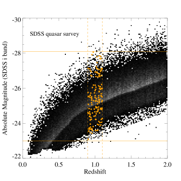
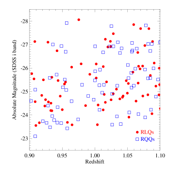
Figure 1: Left: Optical (SDSS $i-$band) absolute magnitude density map of the SDSS quasar sample as a function of redshift. The orange dots are the RLQs and RQQs included in the $z\approx 1$ sample. Selecting the sample at $z\approx 1$ ensures that we have the maximum coverage in luminosity while still probing enough volume to sample the bright end of the luminosity function, where most of the quasars at higher redshift lie. Right: Optical absolute magnitude (SDSS $i-$band) plotted against redshift for the quasars of our sample. RLQs are shown with red circles and RQQs with open blue squares.

In this paper, we present Herschel photometric observation using both Photodetector Array Camera (PACS) at 70 and 160 $\mu$m and the Spectral and Photometric Imaging Receiver (SPIRE) at 250, 350 and 500 $\mu$m for a $z\sim 1$ benchmark sample of 173 AGN. We additionally present the SMA radio interferometer observations at 1300 $\mu$m of the RLQs sample in order to investigate the radio-jet synchrotron contamination of the FIR emission. The paper is structured as follows. In Section 2 we describe the sample selection, the Herschel and SMA observations that we carried out, and the steps used for measuring the flux densities in the observed bands. BH and host galaxy properties and analysis are presented in Section 3. Sections 4-6 present our results on the star formation dependence on AGN luminosity, radio jets and orientation, respectively. In Section 7 we list and discuss our conclusions. Throughout the paper we use the cosmological parameters $H_{\rm 0}=70~{}{\rm km~{}s^{-1}~{}Mpc^{-1}}$, $\Omega_{M}=0.3$ and $\Omega_{\Lambda}=0.7$, and we follow the conversion from FIR luminosities of Kennicutt (1998) when deriving SFRs.

2 DATA

The data presented in this paper consist of Herschel-PACS and SPIRE images of 173 AGN, along with millimetre images taken at 1300 $\mu$m with SMA for the RLQs. The sample is split into three sub-samples, all at the single cosmic epoch of $0.9<z<1.1$: 74 RLQs, 72 RQQs and 27 RGs. This redshift range is convenient because, as shown in Fig. 1, the SDSS survey allows us to probe over 5 magnitudes in quasar optical luminosity. This sample thus enables us to decouple luminosity generated effects from evolutionary ones, something which has plagued many other flux density limited studies in this area.

This redshift is the minimum at which we have a large enough sample of high luminosity quasars ($M_{i}<-25.0$) which can be compared to the bright quasars found at higher redshifts. Observing both unobscured (type-1) AGN, in the form of quasars, and obscured (type-2) AGN, the RGs, allows us to test AGN unification schemes (e.g. Antonucci, 1993). Details of the selection of the quasars are presented by Falder et al. (2010) while the RG selection is described by Fernandes et al. (2015). The Herschel photometry is provided in Appendix A (Table 2) while a summary of the main properties of the sample objects is given in Appendix A (Table 3). In the next section we give a brief description of the sample criteria as they affect this paper.

2.1 Sample selection

The quasars were selected by their optical colours in the SDSS Quasar Survey (Schneider et al., 2005). The sheer size of the SDSS Quasar Survey allowed us to select a large enough initial sample to define matched samples of RLQs and RQQs. The initial quasar sample was then cross referenced with the NRAO VLA Sky Survey (NVSS; Condon et al., 1998), the VLA FIRST survey (Becker et al., 1995) and the Westerbork Northern Sky Survey (WENSS; Rengelink et al., 1997) to pick out the RLQs and RQQs. Regarding the RLQs in the sample, the initial cross-match was done with the WENSS low-frequency survey (325 MHz). Therefore, the RLQs are selected based on optically thin extended emission, which means that the sample selection should be largely orientation independent. The RGs were selected from the low frequency, (178 or 151 MHz; orientation independent) radio samples of the 3CRR (Laing et al., 1983), 6CE (Eales, 1985), 7CRS (Willott et al., 1998) and TOOT surveys (Hill & Rawlings, 2003). For the 6C objects the redshifts are taken from Best et al. (1996), Rawlings et al. (2001) and Inskip et al. (2005), and for the 6C* and TOOT objects from Jarvis et al. (2001b) and Vardoulaki et al. (2010), respectively. Combining these surveys, 27 RGs are found in the same $0.9<z<1.1$ redshift range as our quasars. The smaller RG sample arises from the limit of the known RG population at $z\approx 1$ at the time the samples were defined.

RLQs were chosen to have a low frequency WENSS (325 MHz) flux density of greater than 18 mJy, which is the $5\sigma$ limit of the survey (see Fig. 2). This selection ensures that the vast majority of the RLQs included are characterized by steep radio spectra, avoiding flat radio spectrum quasars and blazars. Additionally, the low frequency radio flux selection allows us to compare the RLQs to the RGs without a severe orientation bias. Falder et al. (2010) presents a classification of the quasar population into radio-loud and radio-quiet based on the definition used by Ivezić et al. (2002). With the exception of 4 objects all of our RLQs have $R_{i}>1$ where $R_{i}=\log_{10}(F_{\rm radio}/F_{i})$ and $F_{\rm radio}$ and $F_{i}$ are flux densities measured at 1.4 GHz and in the $i-$band respectively, so that the RLQ class we use here maps well onto traditional radio-loud/quiet definitions.

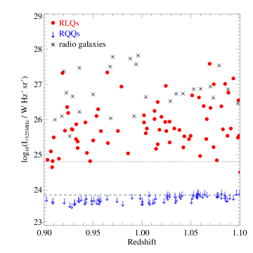
Figure 2: 325-MHz radio luminosity vs. redshift for our sample. RLQs are shown with red circles and RGs with black asterisks. For the RQQs, $5\sigma$ upper limits (extrapolated to rest-frame 325 MHz) from the FIRST survey are shown as blue upper limits. The dashed line shows the average $5\sigma$ limit of the WENSS survey, converted to a luminosity at $z\approx 1$ by assuming $\alpha=0.7$. The dotted line shows the average $5\sigma$ limit of the FIRST survey, extrapolated to 325 MHz. The RQQs were selected to have a radio luminosity falling below this line. The assumed spectral indices for some conversions explains why some objects fall between the lines on this plot.

The RQQs were defined as being undetected by the FIRST survey at the $5\sigma$ level. FIRST was used for this definition because it provides a more sensitive flux density limit than WENSS. Falder et al. (2010) performed a stacking experiment to reveal the average value of the radio power at 1.4 GHz (e.g. White et al., 2007) for the RQQs in our sample. Using this technique they found an average flux density for the RQQs at 1.4 GHz of $0.10\pm 0.02$ mJy (i.e. a 5-$\sigma$ detection). We extrapolate this estimate to a 325 MHz flux density of $0.30\pm 0.06$ mJy assuming a spectral index of 0.7. At $z=1$ this corresponds to a 325 MHz luminosity, $\log_{10}(L_{325{\rm MHz}}/{\rm W~{}Hz^{-1}~{}sr^{-1}})=23.82$.

74 RLQs and 72 RQQs matched in $i-$band magnitude and spanning 5 optical magnitudes were chosen for Herschel follow-up observations. The distribution of optical magnitudes as a function of redshift of the selected sources is shown in Fig. 1. Fig. 2 shows the radio luminosity distribution within the selected redshift range for RLQs and RGs. It is clear that, on average, the RGs are more radio-luminous than the RLQs, albeit with a significant overlap. The results of this selection are further discussed in Section 6. For the RQQs we have placed an upper limit on their radio luminosity (see Fig. 2). In comparison to these limits, RLQs are at least one order of magnitude more radio-luminous than RQQs. The radio luminosity gap between the RLQs and RQQs (Fig. 2) is due to our selection rather than a real radio power dichotomy, because of the different WENSS and FIRST survey depths from which the RLQs are selected.

2.2 Herschel photometry

The data for this work were obtained as part of the Herschel project ‘A benchmark study of active galactic nuclei’ with 55.1 hours of observations allocated. SPIRE observations for 25 objects in our sample were obtained as part of other public Herschel projects (see Table 2). The raw data for these objects were retrieved from the Herschel Science Archive (HSA), and the data reduction was performed as detailed below.

2.2.1 PACS

PACS (Poglitsch et al., 2010) photometric observations at 70 $\mu$m (5 arcsec angular resolution) and 160 $\mu$m (10 arcsec angular resolution) bands were carried out in the scan-map observational mode. A concatenated pair of small map scans of 4 arcmin length, each at two different orientations, was obtained for each source with a total integration time per source of 426-860 secs. The Herschel Interactive Processing Environment (HIPE, Ott, 2010, version 9.1.0) was used to perform the data reduction, following the standard procedures for deep field observations. The high-pass filtering method was applied to create the maps allowing us to minimize the point-source flux loss (Popesso et al., 2012). A preliminary map was created by combining the scan maps which were processed individually for each scan orientation. Using results from Popesso et al. (2012), we choose a masking strategy based on circular patches at prior positions. This method avoids significant flux losses while any other kind of flux losses are independent of the PACS flux densities (Popesso et al., 2012). The final data reduction and mosaicing were then performed using the mask generated in the previous step.

Due to the fact that none of the sources show extended FIR emission and almost $\sim 50$ per cent of the total sample is not detected at $>$3-$\sigma$ level we do not carry out aperture extraction of the FIR fluxes in order to consider all sources equally, even the ones with non-detections, rather than using their $3\sigma$ upper limits. Instead, we directly measure the FIR flux densities from the PSF-convolved images for both bands. We take the flux density to be the value in the image at the pixel closest to the optical position of our targets. We compared the direct flux density measurements to the aperture extraction for the FIR-detected sources and found an insignificant $<5$ per cent difference. The photometric uncertainties of each map were estimated from a set of 500 randomly selected positions (e.g. Lutz et al., 2011; Popesso et al., 2012). The only requirement was that the measured pixels should have a total integration time at least 0.75 times the integration time of that of the source of interest in order to exclude the noisy map edges (e.g. Leipski et al., 2013). The $1\sigma$ photometric uncertainty of the map is taken to be the $1\sigma$ value of the Gaussian fitted to the flux densities measured in these 500 random positions. Measured flux densities are provided in Appendix A (Table 2).

2.2.2 SPIRE

SPIRE (Griffin et al., 2010) photometric observations at 250 (18.2 arcsec angular angular resolution), 350 (24.9 arcsec angular resolution) and 500 $\mu$m (36.3 arcsec angular resolution) were carried out in small scan-map observational mode. The total time per source was 487 secs. Similarly to the PACS data, we used the HIPE standard pipeline to reduce SPIRE data. The FIR flux densities in each band were directly measured from the PSF-convolved images at the pixel closest to the optical position of our targets.

As demonstrated from deep extragalactic observations (e.g. Nguyen et al., 2010), SPIRE maps are dominated by confusion noise at the level of 6-7 mJy beam^-1. The method we have adopted in order to determine the photometric uncertainties in the SPIRE maps is fully described by Elbaz et al. (2011) and Pascale et al. (2011). We have measured the noise level at the position of each source on the residual map produced by removing all individually-detected sources above the detection threshold, and then is convolved with the PSF (Elbaz et al., 2011). On this convolved residual we determined the dispersion of pixel values in a box, around each target, whose size is 8 times the PSF full width at half maximum (the PSF FWHM for the SPIRE passbands is: 18.2 arcsec, 24.9 arcsec, and 36.3 arcsec at 250, 350, and 500 $\mu$m, respectively) (e.g Elbaz et al., 2011; Leipski et al., 2013). The box size was chosen as a compromise between appropriate sampling of local noise variations, surrounding the target, and avoiding inhomogeneities in the exposure time, such as noisy areas at the edges of the map. SPIRE flux densities and their associated errors are provided in Appendix A (Table 2).

2.3 SMA photometry

2.3.1 Synchrotron Contamination

Radio-loud quasars are known to have strong non-thermal beamed core components which could possibly enhance the emission all the way through to the thermal-infrared and possibly the optical waveband (e.g. Blandford & Rees, 1974). Archibald et al. (2001) proposed that high-frequency radio observations are needed to measure the contribution from non-thermal emission to the FIR waveband of radio sources. We expect that our RLQ sample should be dominated by steep-radio-spectrum sources as they are selected on optically thin lobe emission by using low frequency WENSS (325 MHz) observations. RGs are expected to have fainter flat-spectrum core components as a result of their larger angle to the direction of the observer. Given the lack of high-frequency radio observations, the best estimate assumes a spectral index based on the available low-frequency $(<1.4~{}{\rm GHz})$ radio data which could be conservative or a highly uncertain extrapolation to the SPIRE bands.

2.3.2 The SMA sample

For a RLQ to be considered as a candidate for synchrotron contamination at the SPIRE bands, we used the available 1.4 GHz radio observations or the additional data at higher frequencies from the literature as a reference point, and assuming the core spectral shape to be flat, we deem non-thermal contamination to be possible for those objects for which the highest available radio frequency flux falls close to (within the $3\sigma$ error) or above the 500 $\mu$m flux density. We emphasize that this is a very conservative estimate as other authors (e.g. Archibald et al., 2001; Shi et al., 2005; Cleary et al., 2007) fit a parabola, or multiple power-law fits, to the steep-spectrum components in order to take into account possible high-frequency steepening. High-frequency SMA observations at 1300 $\mu$m for the RLQ sample allow us to measure the possible contribution of the non-thermal components to the FIR emission accurately, and minimise the high uncertainties (1-2 orders of magnitudes) caused due to the use of different types of extrapolations (steep-spectrum or flat-spectrum components).

We initially used the existing radio data to assess the potential for synchrotron contamination. For each RLQ we have used an upper (flat-spectrum-dominated; red dashed line) and a lower limit (steep-spectrum-dominated; black dashed line; Fig. 3). We have found that 24 RLQs have potential contamination only when we assume a flat-spectrum core/jet component (Fig. 3; left), and 20 RLQs have potential contamination to their thermal FIR emission from either a steep-spectrum or a flat-spectrum component (Fig. 3; right). For each of these sources, using the 500 $\mu$m flux density as a reference and assuming the spectral shape to be flat, we have estimated the minimum flux density at 1300 $\mu$m in order to have a significant level of non-thermal contamination (Fig. 3; upper limit). For the vast majority of the sources this level is at $\sim 7-10$ mJy.

2.3.3 The SMA observations

We used the SMA (Ho et al., 2004) to observe the 44 RLQ candidates at wavelengths near 1300 $\mu$m (frequencies near 230 GHz) to assess the contribution from synchrotron emission to fluxes measured in the FIR bands. The SMA observations were performed in the 2014-2015 summer and winter semesters, typically in snapshots with 20 minutes on source bracketed by 2 minutes on nearby calibrators to determine complex gains. Many of the observations were executed in available short timeslots before or after other scheduled programmes and shared receiver tunings, correlator setups, as well as flux and passband calibrators. The total bandwidth available was 8 GHz, derived from two sidebands spanning $\pm(4-8)$ GHz from the local oscillator (LO) frequency. For each source, flux densities were measured by fitting a point source model to the visibilities using the task uvfit in the Miriad software package. Each source was also imaged in order to confirm the visibility fit results. Table 4 lists the dates of observation, the characteristic atmospheric opacity during the observations, and the fitted flux densities. Variations in sensitivity are due to both weather conditions and the number of array antennas operating at the time of the observations. Overall, 15 sources were detected at the $>4\sigma$ level (a conservative threshold for these snapshot observations). The absolute flux scale has an estimated systematic uncertainty of $\sim 20$ per cent.

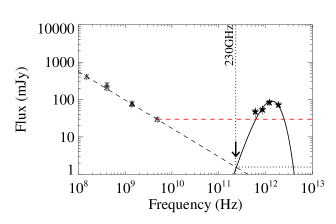
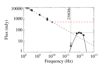
Figure 3: Spectral energy distribution at radio and FIR wavelengths for a sample of the 44 RLQs. Filled black stars: the FIR data (Herschel-SPIRE), Triangles: the radio data (FIRST, NVSS, WENSS and literature), Arrow: the maximum required flux at 1300 $\mu$m in order to not have a significant synchrotron contamination in the FIR bands. Error bars illustrate the $3\sigma$ errors. Black dashed line: Linear fit to radio data; red dashed line: flat radio spectrum; black solid line: grey-body fit; black dotted horizontal line: flat radio spectrum extrapolation at 1300 $\mu$m.

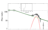
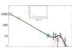
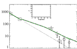
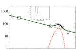
Rejected
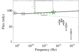
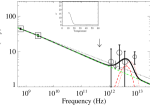
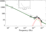
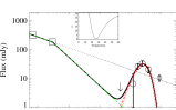
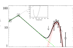
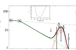
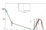
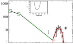
Without contam.

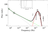
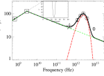
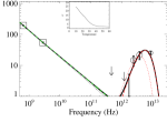
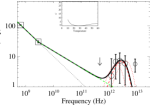
Figure 13: Radio to FIR spectral energy distribution (SEDs, solid black) for representative RLQs observed with SMA. Open squares show the 325 (WENSS) and 1400 MHz (FIRST) radio photometry, open stars the 1300 $\mu$m SMA photometry (arrows indicate the $4\sigma$ upper limit) and open circles the SPIRE and 160 $\mu$m PACS photometry. The 70 $\mu$m PACS photometry is shown with a smaller circle and is not used for the SED fitting. Error bars correspond to $1\sigma$ photometric uncertainties. The radio photometry has been fitted with a broken power-law from 325 to 1400 MHz and from 1400 MHz to 230 GHz (or 1300 $\mu$m; green dashed line) and the FIR photometry with an optically thin modified blackbody component (red dashed line). The dotted black line shows the radio spectrum based on WENSS and FIRST radio observations only. The dotted red lines show the $1\sigma$ blackbody fitting uncertainty. The inner plot show the blackbody fitting $\chi^{2}$ value as a function of dust temperature. The SED plot are arrange in terms of non-thermal contamination at 1300 $\mu$m, from top to bottom. The top panel shows RLQs that have been rejected from our sample, the middle panel RLQs without significant synchrotron contamination at the FIR bands and the bottom panel RLQs in which the 1300 $\mu$m emission is dominated by the thermal component.

Using the SMA observations we have classified the 44 sources identified as having possible synchrotron contamination into two categories. In the first category, we have identified 14 sources with significant synchrotron contamination. All of these sources have been rejected from our sample and from further analysis. The vast majority of them (10) were detected at $>4\sigma$ with the SMA with some extreme cases reaching even $S_{\rm 1300\mu m}\approx 200$ mJy. Some representative examples of the SEDs from this group are presented in Fig. 13. In this category the SMA flux densities exceed the linear extrapolation from the lower-frequency radio data for 8 sources (three are upper limits), for three sources they follow the linear prediction, while for the last three sources they indicate the need of a steeper-spectrum radio component at the higher frequencies. However, even in the last two cases, the contamination to the FIR band is significant and therefore these sources have also been excluded from this work.

In the second category we have classified 30 sources without significant synchrotron contamination. For four cases there is a clear SMA detection at $>$4$\sigma$ while all the other observations indicate an upper limit. For this group of sources, the SMA data exceed the linear extrapolation in seven cases (all of them are upper limits) while in 18 cases they indicate the need of a steeper-spectrum radio component at the higher frequencies. Examples of the SEDs from this group are also presented in Fig. 13.

Overall, we have rejected 17 RLQs from our sample, 14 based on their SMA observations, while three additional sources were classified as flat-spectrum RLQs or blazars based on literature radio observations and rejected ([HB89] 0906+015, SDSS J133749.63+550102.2, SDSS J161603.76+463225.2). As we describe in Section 3.2, there are no particular trends for the sources excluded from our sample and they do not affect the sample matching between RLQs and RQQs.

From our results, it is clear that high-frequency radio observations for similar studies are crucial as the linear extrapolation from lower frequencies works only for $\sim 20$ per cent of the sources. Although most of the cases indicate that the steep-spectrum synchrotron component is likely to fall more quickly at higher frequencies, we find that in $\sim 30$ per cent of the SMA observed sources a high-frequency core radio component is required to describe the radio spectrum. This would also agree with recent findings (e.g. Whittam et al., 2013, 2015). We note that almost half of these SMA observations are upper limits. Radio core variability might be responsible for some of these strong high-frequency components (e.g Barvainis et al., 2005).

3 The black hole and host galaxy properties

In this section we describe how the key parameters for the analysis of this paper are derived, namely BH and stellar masses, Eddington ratios, bolometric luminosities and FIR luminosities. We further explore the importance of AGN contamination in the form of hot dust around the putative torus at FIR wavelengths comparing their FIR colours against normal galaxies. We finally study the correlation between the radio and FIR emission, examining at the same time whether some of the radio emission could be the result of star formation, rather than AGN activity.

3.1 Stellar and black hole mass

Early studies (e.g. Kormendy & Richstone, 1995; Magorrian et al., 1998) suggest a correlation between galaxy bulge and its BH mass. The ratio of the so-called $M_{\rm BH}$-$M_{\rm bulge}$ relation (Magorrian et al., 1998) was estimated to be approximately 0.6 per cent. In the same context, more recent studies using nearby galaxy samples (e.g. Häring & Rix, 2004) find that the median BH mass is $0.14\pm 0.04$ per cent of the bulge mass.

For the quasars in this sample, the BH masses are computed using the virial estimator and the Mgii line at 2800 Å using SDSS spectroscopy, a technique described by McLure & Jarvis (2002), and based on work of McLure & Dunlop (2004). As the H$\beta$ line moves out of the optical window, we have to rely on the Mgii line for AGNs at $z>0.7$ (e.g. Wang et al., 2009). BH masses for the quasars are given in Table 3. We can use the BH mass of the quasars in the sample, along with the $M_{\rm BH}$-$M_{\rm bulge}$ relation to estimate the stellar mass of the galaxy. Despite the convenience of calibrating and using these virial estimators, one must keep in mind that the estimates of these lines are uncertain, potentially by as much as 0.4 dex (e.g. Shen et al., 2011), due to the systematics involved in the calibration and usage (e.g. Jarvis & McLure, 2002, 2006; Marconi et al., 2008; Kelly et al., 2009). We assume that there is no significant evolution of the $M_{\rm BH}$-$M_{\rm bulge}$ relation at $z\approx 1$ from the local relation and thus use $M_{\rm BH}\sim 0.0014M_{\rm bulge}$. Indeed, studies on $z\leq 1$ RLAGN BH-bulge mass relation have found that the estimated ratio lies within the uncertainties of that found in the local Universe (e.g. McLure et al., 2006). Although evolution in the $M_{\rm BH}$-$M_{\rm bulge}$ relation of about 0.2 dex at $z\approx 1$ has been claimed in some papers (e.g. Merloni et al., 2010), that would not significantly add to the uncertainties and would not affect the results of this work, as all of the AGN are selected in a very small redshift range.

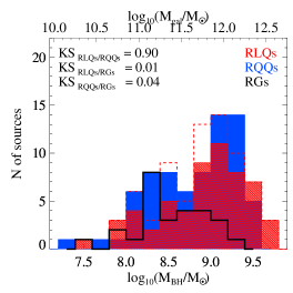
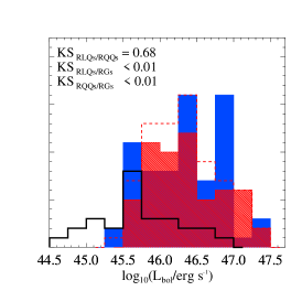
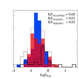
Figure 4: Distributions of BH mass, $M_{\rm BH}$, bolometric luminosity, $L_{\rm bol}$ and Eddington ratio, $\lambda_{\rm Edd}$, for RLQs (red filled), RQQs (blue filled) and radio galaxies (black line). The total RLQ population, including the sources with significant synchrotron contamination is also presented with dashed red lines. In the last panel, the Eddington ratio distribution obtained with both methods of calculating for radio galaxies is presented (dotted black line considering only the accretion energy and solid black line including also the jet mechanical energy). Note the significant increase of the total accretion energy.

For the RGs in our sample, because the broad-line region is obscured, we do not have BH mass estimates as we did for the quasars. For this reason, we use the stellar mass of the galaxy, $M_{\rm gal}$, determined by the SED fitting of Fernandes et al. (2015) for the same radio galaxy sample as used in this work. Fernandes et al. (2015) used the same BH-bulge mass relation (Häring & Rix, 2004) in order to calculate the BH mass of the radio galaxy sample. The implied $M_{\rm BH}$ are given in Table 3. The radio galaxies in our sample have BH masses in the range $10^{7.5}-10^{9.4}~{}M_{\odot}$ (corresponding to $M_{\rm gal}=10^{10.3}-10^{12.0}~{}M_{\odot}$) while the quasars have $10^{7.2}-10^{9.7}~{}M_{\odot}$ (corresponding to $M_{\rm gal}=10^{10.1}-10^{12.4}~{}M_{\odot}$). These are consistent with the range of values found in the literature for similar objects (e.g. McLure & Dunlop, 2004; McLure et al., 2006; Seymour et al., 2007; Salviander et al., 2007).

To test whether the BH and stellar mass distributions differ between the three populations we conducted a Kolmogorov-Smirnov (K-S) test for each pair. The test suggested that the BH masses for the RLQs and RQQs samples are not significantly different. The K-S test gives a result that corresponds to a probability, $p=0.90$ under the null hypothesis (i.e. they are statistically indistinguishable). The mean BH masses are $\langle\log_{10}(M_{\rm BH}/M_{\odot})\rangle=8.87\pm 0.06$ for the RLQs and $\langle\log_{10}(M_{\rm BH}/M_{\odot})\rangle=8.81\pm 0.06$ for the RQQs so the means of the two samples are consistent and well within 1-$\sigma$ of each other.

In contrast, the RG sample could not be selected to match the quasar sample in absolute optical magnitude. The RGs have nominally lower mean BH masses $\langle\log_{10}(M_{\rm BH}/M_{\odot})\rangle=8.53\pm 0.08$; a K-S test comparing to the quasar sample returns 0.01 probability under the null hypothesis, a marginally significant result. Selection effects might also contribute to the observed differences (e.g. RGs are selected from radio surveys without a pre-requisite to be optically bright). We further discuss these effects in Section 6. The distribution of BH masses is shown for all samples in Fig. 4.

3.2 Accretion rate

In order to make an estimate of the AGN power for the radio galaxies an estimate of the bolometric radiative power of the AGN, $L_{\rm bol}$, is required. For the radio galaxy sample, we adopted the values of $L_{\rm bol}$ calculated by Fernandes et al. (2015) from the rest-frame 12$\mu$m luminosity, using a bolometric correction of 8.5 (e.g. Richards et al., 2006), $L_{\rm bol}=8.5\lambda L_{12\mu\rm m}$. The bolometric luminosity for the quasar sample has been computed from the 3000 Å luminosity ($L_{3000}$) using the SDSS spectral fits and a bolometric correction of 5.15 from the composite SED in Richards et al. (2006), $L_{\rm bol}=5.15\lambda L_{3000}$. Fernandes et al. (2011) have computed the bolometric luminosity for the quasar sample based on the rest-frame 12$\mu$m luminosity, following the same method as the one applied for the radio galaxies. Their results suggest no systematics related to methodology or calibration when optical photometry is used for bolometric luminosity estimates.

The bolometric luminosity is proportional to the accretion rate of the BH, $\dot{M}$, and to the fraction of accreted mass that is radiated, i.e. the radiative efficiency, $\epsilon$, through the expression:

$$L_{\rm bol}=\epsilon\dot{M}c^{2}.$$ (1)

Assuming that $\epsilon$ takes the fiducial value of 0.1 (e.g. Marconi et al., 2004; Shankar et al., 2004; Martínez-Sansigre & Taylor, 2009), we determine the accretion rate of our sources using their estimated bolometric luminosity.

With both the BH mass and the accretion rate, we can estimate the Eddington ratio of the sources in our sample. The Eddington luminosity, $L_{\rm Edd}$, corresponds to a maximum accretion rate which a black hole can reach, without preventing further accretion onto it. This energy is a function of the black hole mass of the system and is given by $L_{\rm Edd}=1.3\times 10^{31}(\frac{M_{\rm BH}}{M_{\odot}})~{}{\rm W}$. The Eddington ratio, $\lambda$ is therefore simply,

$$\lambda\equiv\frac{L_{\rm bol}}{L_{\rm Edd}}.$$ (2)

Although for SMBHs accreting at a high fraction the Eddington ratio can be defined as in equation 2, for radio galaxies, especially those with SMBHs accreting at very low rates (e.g. low-excitation galaxies; LEGs), the contribution of the jet mechanical energy in the output of the accretion energy should be considered for the definition of the Eddington ratio. In this case, the total energy from the black hole accretion should equal the sum of the radiative luminosity and the jet mechanical luminosity (e.g. Hardcastle et al., 2007; Best & Heckman, 2012). Including the contribution of the jet power, $Q_{\rm jet}$, the Eddington ratio is given by

$$\lambda_{\rm rad+mec}=\frac{L_{\rm bol}+Q_{\rm jet}}{L_{\rm Edd}},$$ (3)

where $\lambda_{\rm rad+mec}$ is the Eddington ratio accounting for both the radiative energy and the jet mechanical energy. We estimate the jet power using the relation

$$Q_{\rm jet}\simeq 3\times 10^{38}f^{3/2}(L_{\rm 151MHz}/10^{28})^{6/7}~{}{\rm W}$$ (4)

(Willott et al., 1999), where $1\leq f\leq 20$ represents the combination of several uncertainty terms when estimating $Q_{\rm jet}$ from $L_{\rm 151MHz}$. Following Fernandes et al. (2015), we chose $f=10$ as this is the expectation value of a flat prior in natural space. We note that the $Q_{\rm jet}$ contributes significantly to the total power only in the radio galaxies of our sample, which is derived from the $L_{12\mu\rm m}$, and not in the RLQs ($<10$ per cent). The use of any derived radio-luminosity – jet-power relation should be treated with caution, especially for the derivation of the kinematic luminosity function, as they may depend sensitively on selection effects (e.g. Shabala & Godfrey, 2013).

The distribution of bolometric luminosity and Eddington ratio are shown for all samples in Fig. 4. The solid black line is for $\lambda=(L_{\rm bol}+Q_{\rm jet})/L_{\rm Edd}$ and the dotted line for $\lambda=L_{\rm bol}/L_{\rm Edd}$. The Eddington ratio for radio galaxies is significantly higher in the first case, where $\lambda=(L_{\rm bol}+Q_{\rm jet})/L_{\rm Edd}$, and this trend is dominated by high-excitation galaxies (HEGs; see Fernandes et al., 2015; Fig. 7). The red shaded histograms in Fig. 4 represent the RLQ sample after excluding the synchrotron contaminated sources. The total RLQ population is also overplotted (red dashed lines) to stress that no selection biases are introduced in our sample after removing synchrotron contaminated RLQs. No particular trends are observed in any of the distributions between the RLQs and the RQQs as a result of the original matching in absolute optical magnitude and colours.

3.3 FIR emission in RLQs, RQQs and RGs

For each of the quasars in our sample we derive the FIR flux densities in the two PACS and the three SPIRE bands directly from the PSF-convolved images measuring the value at the image pixel closest to the optical position of our targets. The errors are estimated as described in Sections 2.2.1 and 2.2.2. We find that about 33 per cent (43/149) of the QSOs and 8 per cent (2/27) of the RGs in our sample have robust PACS and SPIRE detections. These detection rates are translated to ULIRG-like star formation luminosities suggesting SFRs of hundreds of solar masses per year.

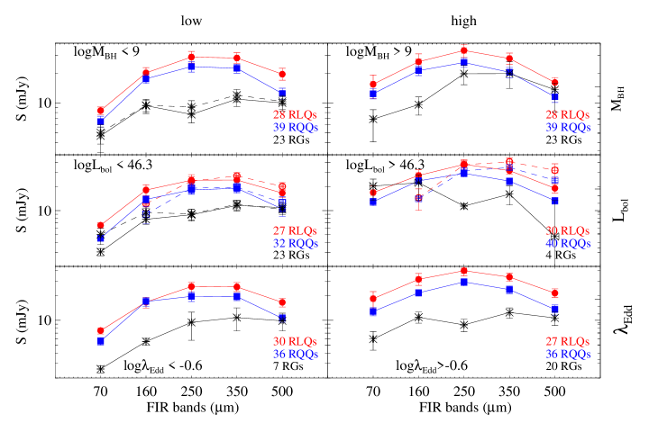
Figure 5: The PACS and SPIRE mean flux densities for RLQS (red filled circles), RQQs (blue filled squares) and RGs (black stars) as a function of BH mass (top panel), bolometric luminosity (middle panel) and Eddington ratio (bottom panel). For low BH mass and bolometric luminosity bins we also present the mean flux density of the total RG population (dashed black line) in order to indicate the contribution of the only four sources found at high bins. We compare our measurements to Kalfountzou et al. (2014b) RLQs (red open circles) and RQQs (blue open squares) with similar bolometric luminosities but different redshift in the middle panels. Table 1 of Kalfountzou et al. (2014b) provides the mean flux densities over their total RLQ sample. Here, for comparison reasons, we present their mean flux densities after removing the RLQs with potential synchrotron contamination.

Table 1: The RLQs, RQQs and RGs FIR average stacked fluxes in the 70, 160, 250, 350 and 500 $\mu$m bandpasses as described in Sectrion 3.3. The AGN populations have been separated into bolometric luminosity bins. The number of objects within each stack is also given.

Class	$\log(L_{\rm bol}/{\rm erg~{}s^{-1}})$	$N$ per bin	Mean flux density (mJy)
			70 $\mu$m	160 $\mu$m	250 $\mu$m	350 $\mu$m	500 $\mu$m
RLQs	$<46.3$	27	$6.55^{+0.44}_{-0.57}$	$18.10^{+3.00}_{-2.72}$	$24.04^{+4.15}_{-3.86}$	$24.15^{+3.76}_{-3.53}$	$16.59^{+1.97}_{-2.04}$
	$\geq 46.3$	30	$16.83^{+3.68}_{-4.22}$	$27.55^{+4.85}_{-4.85}$	$37.89^{+4.65}_{-4.82}$	$31.72^{+3.41}_{-3.24}$	$19.05^{+2.50}_{-2.51}$
RQQs	$<46.3$	32	$4.53^{+0.31}_{-0.45}$	$13.83^{+1.48}_{-1.43}$	$18.17^{+2.06}_{-2.17}$	$19.04^{+2.44}_{-2.60}$	$10.48^{+1.64}_{-2.01}$
	$\geq 46.3$	40	$12.93^{+1.31}_{-1.42}$	$23.58^{+2.20}_{-2.11}$	$29.28^{+2.96}_{-3.02}$	$23.42^{+2.17}_{-2.47}$	$13.33^{+1.21}_{-1.30}$
RGs	$<46.3$	23	$3.04^{+0.31}_{-0.32}$	$7.78^{+0.98}_{-1.04}$	$8.88^{+1.50}_{-1.52}$	$11.60^{+1.72}_{-1.76}$	$10.90^{+1.67}_{-1.49}$
	$\geq 46.3$	4	$20.32^{+4.50}_{-6.96}$	$22.30^{+5.58}_{-8.75}$	$11.39^{+0.83}_{-0.83}$	$16.05^{+4.31}_{-4.31}$	$4.73^{+8.63}_{-8.63}$

We have separated the RLQ and RQQ samples in bolometric luminosity, BH mass and Eddington ratio bins to examine whether the fluxes vary. Within each bin we stack PACS and SPIRE residual maps at the optical position of the AGN from which we derive the mean flux densiy in all FIR bands. We then average the stacked fluxes with the fluxes of the detected ($>3\sigma$ significance level) sources, weighting by the number of sources (e.g. Elbaz et al., 2011; Santini et al., 2012; Rosario et al., 2013). The estimates for each band and bin are shown in Fig. 5. Errors have been estimated by applying the bootstrap technique using randomly selected galaxies from within each bin. The advantage of bootstrapping is that no assumption is made on the shape of the flux distribution. Radio galaxies have significantly lower mean flux densities compared to RLQs and RQQs with a K-S test probability of $p<0.05$. The only exception is the 500 $\mu$m band which might indicate some contribution from synchrotron contamination, or confusion bias, or a combination of them in the case of RGs. This contamination may extend to even lower wavelength bands (e.g. 350 $\mu$m and 250 $\mu$m). Regarding the total quasar sample, the mean flux density appears to increase at high $M_{\rm BH}$, $L_{\rm Bol}$ and $\lambda_{\rm Edd}$. Comparing the RLQs to the RQQs we see that at low $M_{\rm BH}$, $L_{\rm Bol}$ and $\lambda_{\rm Edd}$ RLQs have higher flux densities in all SPIRE bands and all bins, these differences seem to become more significant at the high $M_{\rm BH}$, $L_{\rm Bol}$ and $\lambda_{\rm Edd}$. As no obvious differences are found for the RLQs and RQQs between bolometric luminosity, BH mass and Eddington ratio bins, we give in Table 1 the mean flux estimations from each band and population only for high and low bolometric luminosity bins. We used a black-body modified by frequency-dependent emissivity component (see Section 3.5) to convert the the mean FIR fluxes from our stacked images to mean integated 8-1000$\mu$m far-infrared luminosities for different bolometric luminosity bins. The results are presented in Teble B1.

The stacking method assumes implicitly that the sources in the map are not clustered. It has been shown that this might not be the case for wide PSF (e.g. Béthermin et al., 2010; Penner et al., 2011) with various stacking methods taking this into account also for Herschel beams (e.g. Magnelli et al., 2014). However, with the Spitzer and Herschel beams, it has been shown that the effects of clustering on the stacking are not important (less than 15 per cent; Bavouzet et al., 2008; Fernandez-Conde et al., 2008, 2010; Cao Orjales et al., 2012). In addition, Cao Orjales et al. (in prep.), found on average a small overdensity of Herschel detected star-forming galaxies for the same sample of sources. Once these sources are accounted for, consist of $\sim 0.4$ star-forming galaxies in every AGN field. This overdensity appears to be relatively uniform for both RLQs and RQQs and extends out to the Mpc-scale.

How do these results fit with our previous work? For purposes of comparison we have overplotted in Fig. 5 the mean flux densities obtained by Kalfountzou et al. (2014b), hereafter K14b, (dashed lines) for low and high optical luminosity RLQs (red circles) and RQQs (blue squares). We note two main differences between our current results and those of K14b. Although in the low bolometric luminosity sample of K14b the mean redshift is $z\approx 0.9$, so that we do not expect the evolution effects to significantly change the mean properties, almost all the quasars with high bolometric luminosities have $z>1.0$ up to $z\approx 3$. Therefore, we have converted the mean fluxes of the K14b to the $z\approx 1$ rest-frame. A ratio method was applied in order to derive the k-corrections between the FIR flux densities of a Mrk 231 greybody template ($T=44.75$ K, $\beta=1.55$, constraining 32 data points so to exclude a contribution from AGN-heated dust emission) placed at the redshift of the QSO and the FIR flux density of the QSO. The new flux densities were stacked as described above. Additionally, due to the much larger sample of RQQs in K14b ($>10$ times larger than this work) the uncertainties of this sub-class are expected to be higher in the present paper. Fig. 5 suggests that at low bolometric luminosities, our results are in excellent agreement, at least for the SPIRE bands. The disagreement between our PACS flux densities and those used by K14b is not unexpected since H-ATLAS PACS observations are about 5 times less sensitive than our observations (Ibar et al., 2010). Despite the similar trends, the differences between the RLQ and RQQ populations were more significant in K14b due to the smaller uncertainties for the RQQs. On the other hand, for the high bolometric luminosity bin, both H-ATLAS/SDSS RLQs and RQQs show significantly higher flux densities than the sample in this work, especially at 350 $\mu$m, with a characteristic shift of the the mean peak to the 350 $\mu$m band, indicating colder dust temperatures. These differences provide evidence for the evolution of the FIR emission between $z\approx 2.0$ and $z\approx 1.0$ high bolometric luminosity quasars. That would be expected if QSOs’ host galaxies are evolving with cosmic time in the same way as the general galaxy population (e.g. Madau & Dickinson, 2014).

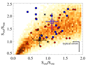
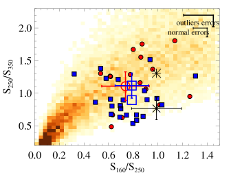
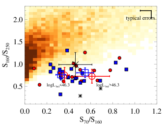
Figure 6: SPIRE and PACS colour-colour diagrams of the AGN in our sample. Small symbols indicate the FIR detected AGN (RLQs = red circle, RQQs = blue squares, RGs = black stars). Detected sources have been selected by imposing a $3\sigma$ cut in each band, excepting 70 and 500 $\mu$m where we use a $2\sigma$ cut due to the low detection rates. Their typical $1\sigma$ errors are also presented in each panel. Stacked measurements for all AGN classes are shown as large symbols with their $1\sigma$ errors. The background density map indicates the colour-colour spaces of our $10^{6}$ randomly generated model SEDs. The darker colours of the density map correspond to denser regions. At the bottom panel, the mean values correspond to the low and high bolometric bins as indicated.

3.4 The FIR colours of RLQs, RQQs and RGs

We now investigate the FIR colours of our sample of AGN. A straightforward approach towards exploring the effect of AGN light on FIR emission is to compare the FIR colours of AGNs against a control sample consisting of galaxies not hosting AGNs. AGN radiation field can heat the dust resulting in systematically warmer temperatures and causing the SED to flatten out at long IR wavelengths which, in turn, leads to bluer FIR colour in galaxies with a significant AGN contamination in the FIR.

In Fig. 6, we compare the FIR colours of the detected AGN sub-sample and the stacked values of the total sub-samples (large symbols) to the FIR colours of $10^{6}$ randomly generated modified black-body, single dust temperature $T_{\rm d}$ spectra models, with a frequency dependence of $\epsilon_{\nu}\propto\nu^{\beta}$. In generating these models, we follow the method of Amblard et al. (2010) considering uniformly distributed dust temperatures from 10 to 60 K, emissivity parameter $0<\beta<2$ and redshift range similar to our sample ($0.9<z<1.1$). In order to consider for flux uncertainties in the colour-colour diagram, we have broadened the SED tracks by adding an extra Gaussian standard deviation of 10 per cent to the model fluxes. Thus, the choice of emissivity parameter would make just a minor difference.

As shown in Fig. 6 (top), we find that in the SPIRE-only colour diagram the colours of the sources are well within the limits defined by the randomly generated model. This is the case for all AGN sub-classes of our sample and also for the individually SPIRE-detected AGN and the mean values. We find no significant dependence of SPIRE colours on any of the AGN associated parameters (e.g. BH mass, bolometric luminosity, Eddington ratio) for each of the AGN sub-classes, so we only present the mean colour-colour values for the total RLQ, RQQs and RG populations. This result, along with the similarity between the AGN SPIRE colours and the model, indicates that SPIRE bands are not significantly affected by emission from the torus (or hot dust surrounding the AGN). Although both quasars’ and radio galaxies’ mean colours lie inside the model tracks, the mean colour of the RGs is shifted from that of the bulk of the model galaxies and the quasars, indicating that it is possible that RGs are associated with redder colours, and therefore cooler dust, or be affected by synchrotron contamination.

Similarly, Fig. 6 (middle) shows that the 160-$\mu$m band does not suffer from torus emission contamination, as the quasars’ and RGs’ $S_{160}/S_{250}$ colours are similar to those of the models. We find that a few individually detected sources lie outside the model set of tracks. However, these outlier sources might be caused by the fractionally larger flux errors of the PACS band, or some of them (mainly RQQs; see blue outliers top panel) are associated with very strong 350-$\mu$m emission suggesting colder dust temperatures than the mean QSO population. By and large, most AGNs can safely be assumed to be dominated by cool dust emission in the SPIRE and 160 $\mu$m FIR bands. As in the top panel, the mean $S_{250}/S_{350}$ for the RGs indicates colder dust temperatures. Again, we find no significant dependence of $S_{160}/S_{250}$ on any of the AGN associated parameters.

In contrast, when we examine the PACS 70 $\mu$m colour, we find that most of the individually FIR detected AGN and the stacked mean colours lie outside th limits defined by our model, suggesting that the PACS 70-$\mu$m band may be significantly contaminated by AGN emission. In the Fig. 6 (bottom) the $S_{160}/S_{70}$ - $S_{250}/S_{160}$ colour-colour diagram for SPIRE 250 $\mu$m and PACS bands of our sample are shown. Although the fractionally larger PACS flux errors could explain some of these outliers, it is possible that some of these sources require a second, warmer dust component (e.g. Dunne & Eales, 2001). For the low and high bolometric luminosity sub-samples there is a clear separation, despite the large error bars, in the $S_{160}/S_{70}$ colours. This difference seems to arise from the AGN contamination at 70 $\mu$m ($\sim 35~{}\mu$m at the rest-frame). Indeed, at the redshifts of our sample, the PACS 70 $\mu$m contains the longer wavelengths of the torus emission (e.g. Mullaney et al., 2010; Xue et al., 2010). If this is the case, then the strong correlation between the 70-$\mu$m emission and AGN emission found for powerful AGN (e.g. Dicken et al., 2009) could be explained by the heavy torus contamination. For this reason, the 70-$\mu$m emission is not used for the FIR luminosity calculation (see Section 3.5). On the other hand, the $S_{250}/S_{160}$ ratio seems to be unaffected by the AGN emission, indicating that 160-$\mu$m emission is largely generated by cold dust, heated by star formation.

3.5 SED fitting

As discussed in the previous section, we expect that the rest-frame FIR emission (160-500 $\mu$m) is mainly generated by cold dust heated by star formation in the AGN host galaxy. Therefore, we interpret the FIR emission as being powered by star formation (e.g. Rowan-Robinson, 1995; Schweitzer et al., 2006; Netzer et al., 2007), and we represent it with a black-body modified by frequency-dependent emissivity component (Hildebrand, 1983), given by

$$S_{\nu}\propto B_{\nu}(T)\nu^{\beta},$$ (5)

where $B_{\nu}$ is the Planck function, $T$ is the effective dust temperature and $\beta$ is the dust emissivity index. Since $T$ and $\beta$ are degenerate for sparsely sampled SEDs, we reduced the numbers of free parameters by fixing the dust emissivity. Using a range $1.4<\beta<2.2$ (see Dye et al., 2010; Hardcastle et al., 2010; Smith et al., 2013, e.g.) we find that the best-fitting model returns lower $\chi^{2}$ values for a fixed $\beta=1.6$ dust emissivity for all AGN populations in the sample. The selection of $\beta=1.6$ is consistent with the work of Dye et al. (2010). The remaining two free parameters are the cold dust temperature, which we have varied over the range $10<T({\rm K})<60$ and the flux normalization of the modified black-body component.

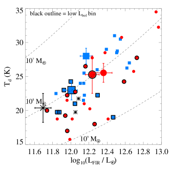
Figure 7: FIR luminosity (${\rm L_{FIR}}$) versus dust temperature ($T_{\rm d}$) for individually FIR detected AGN and weighted mean values when the RLQs and RQQs are divided into bolometric luminosity bins. For RGs, we present the weighted mean values for the total population as all the sources but 4 belong to the low bolometric luminosity bin. Black outline indicates the sources and the weighted mean values for the low bolometric luminosity bin. Colours and symbols are similar to Fig. 6. The black lines correspond to the dust mass ($M_{\rm d}$) estimates based on the ${\rm L_{FIR}}$ - $T_{\rm d}$ relation ${\rm L_{FIR}}\propto M_{\rm d}T_{\rm d}^{4+\beta}$, assuming $\beta=1.6$, for dust masses of $10^{7}$, $10^{8}$ and $10^{9}~{}{\rm M_{\odot}}$.

For each source we estimated the integrated FIR luminosity ($8-1000~{}\mu$m) using a modified black-body fitting with the best fit temperature. The dust temperature was obtained from the best fit model derived from minimization of the $\chi^{2}$ values. The uncertainty in the measurement was obtained by mapping the $\Delta\chi^{2}$ error ellipse, allowing the individual photometric measurements to vary within their $1\sigma$ ranges of uncertainty. In addition to the integrated FIR luminosity we calculate the mass of the FIR emitting dust component using

$$M_{\rm dust}=\frac{1}{1+z}\frac{S_{250}D_{L}^{2}}{\kappa B(\nu,T)},$$ (6)

where $S_{250}$ is the 250 $\mu$m observed flux, $D_{L}$ is the luminosity distance, $\kappa$ is the dust mass absorption coefficient, which Dunne et al. (2011) take to be $0.89~{}{\rm m^{2}~{}kg^{-1}}$ and $B(\nu,T)$ is the Planck function.

In the case of RGs and RLQs, we also extend the modified black-body model to the radio bands with either a power-law slope $S_{\nu}\propto\nu^{-\alpha}$, with $\alpha$ estimated from 325 MHz and 1.4 GHz radio observations or, a broken power-law for the RLQs with available SMA observations at 1300 $\mu$m. In the second case, the broken point is fixed at the 1.4 GHz. Examples of the SED fits are presented in Fig. 13.

As the majority of the sources are undetected at the $3\sigma$ limit in all Herschel bands, in addition to probing the properties of the individually FIR-detected objects, we carry out two different stacking approaches for the estimation of the FIR luminosities. In the first approach, we follow the method of Hardcastle et al. (2010, 2013) regarding the consideration of the undetected sources ($<3\sigma$) in our sample. We determine the luminosity of each source from the Herschel flux densities (excluding 70 $\mu$m), even if negative, on the grounds that this is the maximum-likelihood estimator of the true luminosity, withouth making any assumption for their distribution in contrast to Hardcastle et al. (2010). We then take the weighted mean of the parameter we are interested in within each bin. For the mean calculation, the luminosity is weighted using the errors calculated from $\Delta\chi^{2}=2.3$ and the errors on the stacked parameters are determined using the bootstrap method. We use the same bins across the AGN sub-classes in order to facilitate comparisons. In the second approach, we consider the FIR upper limits of each source as tentative detections, and estimate upper limits for the ${\rm L_{FIR}}$ using the procedure adopted for the objects detected in Herschel bands. The motivation for the second approach is the comparison of our results with recent works that follow similar statistical analysis (e.g. Drouart et al., 2014; Podigachoski et al., 2015). The mean far-infrared luminosities for both stacking and statistical methods are given in Appendix B. We found that our main results are consistent with the results we obtain when using the direct stacking analysis (Section 3.3). As also found in Kalfountzou et al. (2014b), we found small but insignificant differences between the two methods, so for convenience we present here only the results of the weighted first approach. For the estimation of the mean FIR luminosity we again use two approaches. The first one is a weighted mean, each FIR luminosity is using the errors calculated from the $\Delta\chi^{2}=2.3$ of the fitting. The second one is a simple median. Both are in a good agreement as we present in the following plots.

Fig. 7 shows the FIR luminosity and dust temperature ($T_{\rm d}$) plane divided into dust mass ($M_{\rm d}$) regions based on the $L_{\rm FIR}\propto M_{\rm d}T_{\rm d}^{4+\beta}$, assuming $\beta=1.6$, for the FIR-detected AGN of our sample (similar cuts to Fig. 6 top) and the weighted mean values for the total sample and for each sub-class. The sources have been additionally divided into bolometric luminosity bins as specified in Table 1. Both types of quasars show high FIR luminosity with most of the detected sources and the weighted mean values having $L_{\rm FIR}>10^{12}~{}{\rm L_{\odot}}$, characterizing them as ultra-luminous infrared galaxies (ULIRGs). The weighted mean FIR luminosity of the RGs is significantly lower, even compared to the low bolometric luminosity quasars. Similar differences are also found for low BH mass and Eddington ratio bins. Comparing the FIR luminosity of the RLQs and RQQs it is notable that RLQs have higher weighted mean FIR luminosity than RQQs in both bolometric luminosity bins at $>1\sigma$ level with a significance of $p=0.014$. Similar trends are also found for BH masses and Eddington ratio.

As already indicated from the colour-colour plots, RGs show lower dust temperatures than both RLQs and RQQs (by about 5K) at a significance level of $p=0.036$ and $p<0.001$, respectively, under a K-S test. For all AGN subclasses and bins, the weighted mean values follow the $10^{8}~{}{\rm M_{\odot}}$ dust mass curve, with the exception of high bolometric luminosity RQQs which have slightly lower weighted mean dust mass (and higher dust temperature). Most of the FIR-detected RLQs lie between the $10^{8-9}~{}{\rm M_{\odot}}$ dust mass curves. This mass range is comparable to that obtained for submillimetre galaxies (e.g. Santini et al., 2010) at similar redshifts to our sample.

3.6 FIR-radio correlation

In this section we determine whether some of the radio emission could be the result of star formation, rather than AGN activity, by comparing the observed radio flux with that predicted from the FIR/radio correlation. As the high detection rates and the weighted mean FIR flux densities in the RLQ sample indicate, almost 50 per cent of the population is expected to have high star formation activity. High star formation activity, at the level of ${\rm L_{FIR}}>10^{11}L_{\odot}$, could result in radio emission up to $10^{24}~{}{\rm W~{}Hz^{-1}}$ at 1.4 GHz, which is the detection level of our RLQs. We additionally investigate whether radio excess (i.e. radio emission associated with radio jets) correlates with star formation as one would expect assuming a jet-induced star formation (positive feedback) model.

We calculate the ratio between the IR and radio emission ($q$) using the definition given by Helou et al. (1985)

$$q=\log[f_{\rm FIR}/(3.75\times 10^{12}~{}{\rm Hz})]-\log[S_{\nu}({\rm 1.4~{}GHz})]$$ (7)

where $f_{\rm FIR}$ is in units of ${\rm W~{}m^{-2}}$, determined from the Herschel photometry and $S_{\nu}(1.4~{}{\rm GHz})$ is rest-frame 1.4 GHz radio flux density in units of ${\rm W~{}m^{-2}~{}Hz^{-1}}$. We extrapolate the above relation to 325 MHz using the power-law slope $S_{\nu}\propto\nu^{-\alpha}$, with $\alpha=0.7$, typical for star-forming galaxies (e.g. Ibar et al., 2009, 2010; Condon et al., 2013).

In Fig. 8 we show the FIR and the radio 325-MHz luminosities for all of the RQQs (blue upper limits), RLQs (red circles and upper limits for FIR-undetected sources) and RGs (black point stars and upper limits for FIR-undetected sources) in our sample. The diagonal lines represent the mean $q=2.2$ value typically obtained for star-forming/starburst galaxies (e.g. Helou et al., 1985) and also typical radio-quiet AGN (e.g. Padovani et al., 2011; Sargent et al., 2010) and the mean $q=-0.38$ for a sample of radio-loud AGN from Evans et al. (2005). For the separation between ‘radio-normal’ and radio-excess sources we have picked the mean $q=1.2$ value that perfectly separates the RLQs and RQQs in our sample. We note that this is a conservative value compared to previous works (e.g. $q=1.68$; Del Moro et al., 2013, $q_{\rm max}=1.5$; Hardcastle et al., 2010, $q_{\rm max}=1.1$; Jarvis et al., 2010) indicating that above this limit we are predominantly detecting genuine radio-loud AGN.

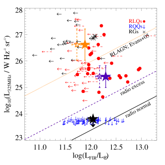
Figure 8: FIR luminosity ($L_{\rm FIR}$) vs. radio 350 MHz luminosity ($L_{\rm 325MHz}$); the orange dotted line corresponds to $q=-0.38$ (average for a sample of radio-loud AGN from Evans et al., 2005); the black solid line corresponds to $q=2.2$ (average for ‘radio-normal’ sources) and the purple dashed line corresponds to $q=1.68$, our selection limit for radio-excess sources. The large filled stars are the weighted mean values of all sources in each region while small open stars with dashed error bars are the weighted median values. No significant differences are found between mean and median estimations. Colours are associated to the lines. For individually FIR detected sources, colours and symbols are similar to Fig. 6. FIR-undetected sources are presented as upper limits. We also include FIR luminosity upper limits (dashed red upper limits) for the 17 RLQs that have been excluded from the sample due to the significant synchrotron contamination at the FIR bands.

The average upper limit $q$ for the RQQs lies near to the ‘radio-normal’ diagonal line, taking into account that all the RQQs radio luminosities shown are the $5\sigma$ limits. All but one of the RGs in our sample is found above the RLAGN $q=-0.38$ diagonal line (orange dotted line) while about 70 percent of the RLQs lie in a region between those occupied by RGs and RQQs. This is consistent with the selection of the RG and RLQ samples. It is clear that the level of radio emission from star formation is insignificant for both RLQs and RGs. All radio-sources are found above the $q=-1.68$ diagonal line suggesting that the radio emission associated with star formation may contribute by a maximum of 10 per cent for the least radio-luminous RLQs.

For each region in Fig. 8, we have estimated the weighted mean FIR luminosity, represented by the large filled stars; orange for the sources in the RLAGN region, purple for the sources in the radio-excess region and black for the radio normal region. As expected based on Fig. 7 the objects in the radio-excess region, which consists only of RLQs, show a higher FIR luminosity. In contrast, the weighted mean FIR luminosity at the RLAGN region is lower than that in both the ‘radio-normal’ and radio-excess regions. Although the RLQs in this region are associated with higher FIR luminosities compared to the RGs, and have about a 50 per cent detection rate, their individually measured FIR luminosities do not exceed the weighted mean FIR luminosity of the radio excess region. Weighted mean values of the total radio population, including both RGs and RLQs, show an anti-correlation between FIR and radio luminosity. Sources with higher radio luminosity show weaker star formation. We can investigate the apparent anti-correlation further considering the individual sources, although the numerous upper limits might affect the the establishment of such a correlation. In order to consider also the sources with FIR upper limits, we use Kendall’s Tau statistical test. For this, the IRAF statistics package, which implements the Astronomical Survival Analysis programs (see Feigelson & Nelson, 1985; Lavalley et al., 1992), was used. This test examines the null hypothesis that no correlation is present between the two variables being tested. For the total radio sample the generalized Kendall’s correlation coefficient is $\tau=-0.13$ with a null hypothesis probability of $p=0.12$, implying no significant correlation. The same trend is observed even if we use, instead, a more outlier-resistant averaging such as the median (open stars).

These results are not affected by the exclusion of the 17 RLQs with strong synchrotron contamination, as it is clear that they follow similar trends with the general RLQs population (see dashed red upper limits in Fig. 8). In addition the mean radio luminosity of the rejected RLQs is $10^{26.10\pm 0.47}~{}{\rm W~{}Hz^{-1}~{}sr^{-1}}$, very similar to the included RLQs population ($10^{25.84\pm 0.41}~{}{\rm W~{}Hz^{-1}~{}sr^{-1}}$). Thus, we do not expect that the rejected sample would affect differently the two regions separated by the Evans et al. (2005) line. Although the upper limit FIR luminosity estimation for the excluded RLQs would be insufficient to draw firm conclusion, especially on account of the strong blazar variability, we could follow a different approach in order to insure that we do not introduce any selection biases rejecting these sources. Assuming that the dust temperature distribution of the excluded sample should be similar to the included RLQs, we use the $250\mu$m flux density, which should be the least contaminated from the synchrotron emission, as a proxy of the FIR luminosity. We found that both the included and the excluded RLQs have very similar median $250\mu$m flux densities, $20.06\pm 4.14$ mJy and $18.46\pm 9.12$ mJy, respectively. If we also consider the excluded RLQs sample for the estimation of the median $250\mu$m flux densities at the ‘RGs+RLQs’ and ‘RLQs’ regions the radio-luminous sources above the Evans et al. (2005) line show significantly lower median $250~{}\mu$m flux densities, $10.55\pm 1.90$ mJy and $19.53\pm 6.51$ mJy, respectively.

To check for the robustness of the differences in the mean FIR luminosity values between the different classes, we carried out the non-parametric Mann-Whitney U test (hereafter referred to as the M-W U test). The M-W U test allows the comparison of two groups without the underlying distribution of the data being necessarily normal. The FIR luminosities of the two groups are significantly different at a $>98.5$ per cent confidence level. In order to account for the upper limits in our sample, we also use statistical methods that are often generalizations of these classical non-parametric test. We use the astronomical survival analysis package (ASURV; Feigelson & Nelson, 1985). Using three different tests, the Gehan’s Generalized Wilcoxon test; the log-rank test; and the Peto and Peto Generalized Wilcoxon test, the difference in the RLs and RLQs distributions of the FIR luminosity is confirmed at $>98.9$, $>99.3$, and $>98.9$ per cent confidence level, respectively.

The fact that high radio luminosity RGs and RLQs (see orange star; Fig. 8), are associated with lower FIR luminosity compared to lower radio luminosity RLQs (purple star; Fig. 8) may indicate two possible physical scenarios. In the first scenario, we can assume that there is a radio-jet power limit above which radio jets suppress the star formation in the host galaxy. That would be consistent with the negative radio-jet feedback scenario (e.g. Croton et al., 2006). In contrast, lower power radio-jets might enhance the star formation (positive feedback) and that would explain the FIR excess between RQQs and RLQs with intermediate radio luminosity, the ones found in the radio-excess region. However, we should expect that these processes are controlled by the gas availability (i.e. galaxy mass). Indeed, RLQs with similar radio luminosities to the RGs have higher FIR luminosities and higher black hole masses. Therefore, we expect that they are hosted by galaxies with larger masses, assuming that the Maggorian relation holds. Although this interpretation could explain the observed differences, the effects of the radio jets cannot be so straightforwardly understood unless we control for galaxy mass. We discuss this scenario further in Section 6. Another important parameter is the environment of these sources, which can lead to a second possible scenario. Taking into consideration that the RGs have been selected from radio surveys whereas the RLQs are optically selected, we might have picked the two populations in either different evolutionary stages or different environments (see the discussion in Section 6). This fact could drive the apparent lower FIR luminosity when we consider both RGs and RLQs.

4 The star formation dependence on AGN activity

Using measurements of FIR luminosity, we will now study the relationship between FIR emission and SMBH accretion. In Fig. 9, the FIR luminosity is plotted against bolometric luminosity $L_{\rm bol}$ with symbols representing both FIR luminosities for individually FIR-detected sources (small symbols) and weighted mean (large open symbols) and median (small open symbols with dashed error bars) values. The $L_{\rm bol}$ is the mean value for the objects in each bin with their associated $1\sigma$ error bars. Different colours are used to represent the different AGN classes. A crucial point of our results is that about 30 per cent of our QSOs are FIR-detected, indicating high FIR luminosities at the level of $L_{\rm FIR}\gtrsim 10^{12}L_{\odot}$. The high FIR emission suggests that starburst activity in 30 per cent of our QSOs has not been quenched yet. These results argue for a scenario in which powerful quasars, on average, have not yet suppressed the star formation in the host galaxy (see Harrison et al., 2012; Rosario et al., 2013; Stanley et al., 2015, e.g. but also Page et al., 2012, e.g.).

To search for possible trends between bolometric and FIR luminosity we performed a correlation analysis on each of the sub-samples. In order to take account of the sources with FIR upper limits, we use the Kendall’s Tau statistical test as described in Section 3.6. This test examines the null hypothesis that no correlation is present between the two variables being tested. The correlation analysis returns $\tau=0.34$ ($p=0.02$), $\tau=0.28$ ($p=0.02$) and $\tau=0.15$ ($p=0.32$) for RLQs, RQQs and RGs, respectively, suggesting a moderately significant correlation over more than 2 orders of magnitude in $L_{\rm bol}$ for both RLQs and RQQs. For RGs no significant correlation is observed over $\lesssim 2$ orders of magnitude.

A correlation between AGN luminosity and host galaxy star formation rate has been reported by several studies of high redshift AGNs and QSOs (e.g Lutz et al., 2008; Shao et al., 2010; Rosario et al., 2012; Rovilos et al., 2012). Netzer et al. (2007) found for luminous PG QSOs that this relationship has a slope of $\alpha\approx 0.8$ (see black dotted line in Fig. 9). Consistent slopes have also been suggested by other authors for mm-bright QSOs at $z\sim 2$ (e.g. Lutz et al., 2008) and X-ray AGN (e.g. Rosario et al., 2012) at least for high AGN luminosities. We note that Rosario et al. (2012) suggested a flatter or even zero slope at low AGN luminosities ($L_{\rm AGN}<10^{44}~{}{\rm erg~{}s^{-1}}$). As these works have selected their AGN samples without any use of radio information, we expect that they are dominated by radio-quiet AGN. Radio-loud AGN are expected to make up to 10 per cent of uniformly selected AGN samples, so they should not significantly affect the estimation of these works.

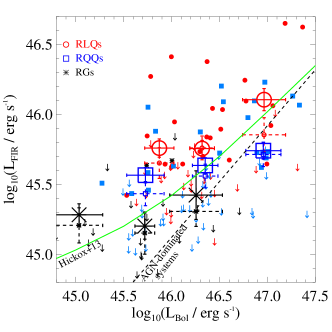
Figure 9: FIR luminosity ($L_{\rm FIR}$) vs. bolometric luminosity ($L_{\rm bol}$) for each AGN class in 3 $L_{\rm bol}$ bins. For RLQs and RQQs each bin contains about 18 and 23 sources, respectively, while for RGs about 9 sources. The large symbols (red circles, blue squares and black stars) are the weighted mean values of each bin for RLQs, RQQs and RGs, respectively. The small open symbols with dashed error bars are the weighed median values. No significant differences are found when the median values are used, apart from the last RLQs bin. For individual sources, colours and symbols are similar to Fig. 6. FIR undetected sources are presented as upper limits. The dashed black line is the correlation line shown by AGN-dominated systems in Netzer et al. (2009). The solid green line show the predictions of the Hickox et al. (2014) fiducial model on BH variability and star formation-AGN connection.

The RQQs of our sample are very similar to that of Netzer et al. (2007), with a good overlap on AGN luminosity up to $L_{\rm AGN}\sim 10^{46.5}~{}{\rm erg~{}s^{-1}}$, while our sample extends to about an order of magnitude higher in AGN luminosity. The correlation between the FIR and AGN luminosity based on the Netzer et al. (2007) QSO sample is presented in Fig. 9. One important difference is the redshift range of the two samples, with the QSOs of Netzer et al. (2007) having $z<0.3$. Notwithstanding this difference, the selection of our sample in a narrow redshift range decouples the evolution effect and makes it perfect for comparison to either lower or higher redshift samples. One can immediately notice from Fig. 9 that the $L_{\rm AGN}$-$L_{\rm FIR}$ correlation is much weaker and flatter than the one proposed by Netzer et al. (2007). The correlation slope for the RQQs of this work is found to be $\alpha\approx 0.26\pm 0.06$. Specifically, the lower $L_{\rm AGN}$ sources in our sample show a weighted mean $L_{\rm FIR}$ of one order of magnitude higher than that implied by the correlation of Netzer et al. (2007) while at higher $L_{\rm AGN}$ they are in better agreement. Such an increase of the FIR luminosity at a fixed AGN luminosity bin with redshift has been suggested by other authors (Rosario et al., 2012; about 0.7 dex from $z\sim 0.3$ to $z\sim 1$ AGN) and it would explain the FIR luminosity difference between our sample and that of Netzer et al. (2007) in fixed $L_{\rm AGN}$ bins. On the other hand, QSO selection at lower redshifts (e.g. $z<0.3$), where the star formation density in the universe is very low, might be affected by Malmquist bias. A similar trend for shallower slope ($\alpha=0.58\pm 0.18$) at similar $L_{\rm AGN}$ and redshift but for X-ray AGN was suggested by Rosario et al. (2012) although the quality of the fit is rather poor. Even in this case, our data suggest a much shallower slope ($\alpha\approx 0.26\pm 0.06$) for the RQQs. Note that even if we include the RLQs the estimated slope can reach a maximum of $\sim 0.32$.

Selection effects that arise from flux limited surveys could influence the observed AGN - FIR luminosity slope (e.g. Shen et al., 2008; Schulze & Wisotzki, 2010; Steinhardt & Elvis, 2010) as the black hole mass is correlated with the stellar mass and this, in turn, with the SFR. The lower luminosity QSOs in our sample contain more systems with lower black hole masses, and thus lower stellar masses which might explain the lower FIR luminosity.

Luminous, high-redshift quasars typically yield lifetimes for luminous accretion of $\sim 10^{6}-10^{7}$ years (e.g. Hopkins et al., 2005; Gonçalves et al., 2008; Shankar, 2010). On the other hand, galactic-scale star formation has a dynamical time of around $10^{8}$ yr. In addition, as FIR emission arises mostly from dust that can be heated by both young and old stars, it can average over timescales of tens to hundreds of Myr, especially in galaxies with star formation at a relatively steady rate over their lifetime. Thus, the weak observed correlation between star formation and BH accretion might be attributed to the timescale difference between the AGN accretion efficiency and star formation variability (e.g. Mullaney et al., 2012b; Chen et al., 2013; Hickox et al., 2014).

From a theoretical point of view, Hickox et al. (2014) suggested a simple model in which accretion and star formation are perfectly connected, but this connection is ‘hidden’ by short-timescale AGN variability over a large dynamic range (see Fig. 9 green solid line). Despite the fact that the model goes through our data points for the individual QSOs, the mean measurements are systematically off-set. Although the model of Hickox et al. (2014) describes well the lack of a strong correlation between $L_{\rm FIR}$ and $L_{\rm AGN}$ for moderate-luminosity AGN and the shift to higher $L_{\rm FIR}$ with redshift as suggested by observational results, it suggests a strong correlation between $L_{\rm FIR}$ and $L_{\rm AGN}$ at high luminosities, in contrast to our results. However, the apparent disagreement could arise from limitations in the simplistic AGN variability model (for a discussion see Hickox et al., 2014) or from the fact that our sample contains exclusively powerful QSOs with high accretion rates. An alternative model, suggested by Aird et al. (2013), assumes that the probability of a galaxy hosting an AGN is determined by a universal specific accretion rate distribution that is independent of host stellar mass or star formation properties. This model would be consistent with the observed weak AGN/star-formation correlation of this work even in the most luminous QSOs.

In Fig. 10 we present the average FIR luminosity of each AGN population, as a function of $M_{\rm gal}$. We have to note that the galaxy masses are not actual stellar mass measurements for our QSOs but they have been estimated based on the black hole measurements assuming a Magorrian relation. This fact may introduce high uncertainties. As expected under the assumption of a hidden QSO – star-formation correlation due to the different timescales of the two phases, we find no correlation for any AGN sub-class between FIR luminosity and stellar mass, in contrast to the result of Mullaney et al. (2012b). The most luminous AGN, like the ones in our sample, are generally missed from small field surveys. However, at redshift $0.9<z<1.1$ they make up to 10 per cent (e.g. Aird et al., 2010) of the total AGN population ($L_{\rm X}>10^{42}~{}{\rm erg~{}s^{-1}}$). Despite their large FIR excess, an order of magnitude in FIR luminosity, their rarity means that they might not significantly change the results found by Mullaney et al. (2012b).

Comparing the average SFRs of this sample to the observed relationship between SFR and stellar mass of normal star forming galaxies, which is known as the “main sequence” (e.g. Elbaz et al., 2007, 2011; Schreiber et al., 2015; Johnston et al., 2015) we can examine whether QSOs have SFRs that are consistent with being selected from the overall star forming galaxy population. To make this comparison we use the Schreiber et al. (2015) definition of the ‘main sequence’ at $z\sim 1$ (see Eq. 9 of Schreiber et al., 2015). They found evidence for a flattening of the main sequence at high masses ($\log_{10}(M_{\rm gal}/M_{\odot})>10.5$), similar to the one observed for the sources in our sample. Note that they use stellar masses up to $\log_{10}(M_{\rm gal}/M_{\odot})\approx 11.5$ to extract their model. Although the weighted mean FIR luminosity of the RGs (large point stars) is consistent with that of star forming galaxies of the same redshift and mass, the weighted mean FIR luminosity for QSOs is systematically higher than the higher end of the FIR luminosity region covered by ‘main sequence’ galaxies. Similar results have recently been reported for luminous, optically selected quasars. This supports the statement that luminous AGNs are more likely to be associated with major mergers (e.g. Ma & Yan, 2015; Dong & Wu, 2016).

Santini et al. (2012) have also reported that, on average, X-ray AGN hosts show somewhat enhanced star-formation activity with respect to a control sample of inactive galaxies, although they found them to be consistent with star forming galaxies. While different interpretations are possible, our findings are consistent with a scenario whereby periods of enhanced AGN activity and star-forming bursts are induced by major mergers (e.g. De Breuck et al., 2005; Elbaz et al., 2011; Sargent et al., 2013).

X-ray and FIR observations have been widely used for the investigation and comparison of the star formation activity in distant AGN and star-forming galaxies (e.g. Shao et al., 2010; Harrison et al., 2012; Mullaney et al., 2012b; Rovilos et al., 2012; Santini et al., 2012; Rosario et al., 2013). They suggest that the sSFRs of AGN are consistent with those of star-forming galaxies, with possible exceptions the luminous AGN (e.g. Rovilos et al., 2012; Treister et al., 2012). Most of these X-ray works investigate the mean SFRs of AGNs that are less luminous than those studied here, and should also include a high fraction of narrow-emission line AGN. Rosario et al. (2013) suggested a baseline model for X-ray broad-emission line QSOs based on which moderate luminosity QSOs are hosted by galaxies that lie on the star-forming mass sequence.

In the case of the RQQs in this work, which are similar only to the most luminous sources of Rosario et al. (2013), we have found a mean positive offset of $\sim 0.4$ dex in $\log L_{\rm FIR}$, which corresponds to the upper limit of the region covered by “main sequence” galaxies. As we see in Fig. 10, the FIR-detected quasars at the $3\sigma$ level (about 30%) are mainly responsible for the SF enhancements compared to the star-forming galaxies, while the upper limits of the FIR-undetected quasars lie well inside the “main sequence”. A possible explanation for the differences between our observations and Rosario et al. (2013) baseline model could arise from the fact that a significant fraction of our RQQs is preferentially in “special” populations such as starburst or major mergers that are associated with higher star formation efficiency (e.g Daddi et al., 2010; Genzel et al., 2010).

Indeed as some studies have suggested, the fraction of quasars hosted by mergers and/or interacting system is about 30 per cent from unreddended quasars (e.g. Dunlop et al., 2003; Floyd et al., 2004), while for red quasars the merger fraction increases to $\sim 85$ per cent. Assuming that the merger fraction might rises with bolometric luminosity (e.g. Hopkins & Hernquist, 2006; Urrutia et al., 2008; Somerville et al., 2008; Treister et al., 2012) that would explain why the mean SFR for our sample, which is more luminous than Rosario et al. (2013), is higher than the one for the inactive galaxies.

These studies imply that the host galaxies of moderate luminous AGN and the most luminous AGN might evolve along different paths. The low and moderate luminous AGNs are fueled by secular processes (e.g. Hopkins & Hernquist, 2006; Jogee, 2006; Younger et al., 2008), while high luminosity AGNs evolve through major mergers and might have a direct link between the black hole growth and bulge growth.

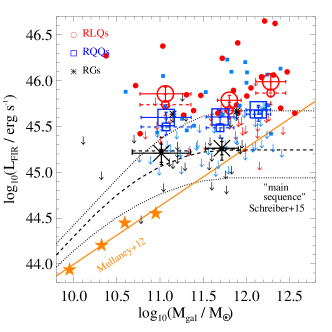
Figure 10: FIR luminosity ($L_{\rm FIR}$) vs. galaxy mass ($M_{\rm gal}$) for each AGN class in 3 $L_{\rm bol}$ bins. Colours and symbols are similar to Fig. 9. The large symbols (red circles, blue squares and black stars) are the weighted mean values of each bin for RLQs, RQQs and RGs, respectively. The small open symbols with dashed error bars are the weighed median values. No significant differences are found when the median values are used. Similar results are obtained even when the median values are used for each bin. The solid orange line and orange stars correspond to the average FIR luminosity and stellar mass for Mullaney et al. (2012) $z\sim 1$ sample of star-forming galaxies. The black dashed line with the associated scatter (dotted black lines) corresponds to the expected ${\rm L_{FIR}}-M_{\rm gal}$ relation for $z\sim 1$ as defined by Schreiber et al. (2015).

5 The dependence of star formation on radio jets

In this section we will discuss the effect of the presence of radio jets in a QSO on star formation activity. As is already clear from the previous section (see Fig. 9), RLQs are associated with higher FIR luminosity than RQQs. This excess is almost constant and independent of AGN properties. Fig. 11 shows the SFR excess, defined as the SFR difference between RLQs and RQQs, for the individual sources in each $L_{\rm bol}$ bin, taking into account the total population (orange filled area) or only the FIR detected QSOs (purple shaded area). Apart from the highest bolometric luminosity bin, where only a few sources are found, the SFR excess is almost constant with $\Delta{\rm SFR}\approx 315~{}{\rm M_{\odot}/yr}$ for the total sample and $\Delta{\rm SFR}\approx 380~{}{\rm M_{\odot}/yr}$ for the FIR-detected QSOs. This excess corresponds to about a factor of two. A similar increase in SFR due to the onset of radio jets has been suggested also by simulations of massive, gas-rich, high-redshift galaxies (Silk & Nusser, 2010; Gaibler et al., 2012).

SFR-enhancing phases in RLQs can be caused due to the formation of bow shocks generated by the jet which compresses the interstellar medium (ISM). Jets create cocoons of turbulent gas surrounding the jet leading to a much more efficient clumping of molecular hydrogen and thus accelerated star formation (e.g. van Breugel et al., 2004; Gaibler et al., 2012; Wagner et al., 2012; Ishibashi & Fabian, 2012). Simulations have shown that, although powerful jets’ interaction with the ISM might be volume limited, the resulting pressure can impact the galactic disk also at larger radii and eventually all of the galaxy (see Gaibler et al., 2012). Thermal or kinetic AGN feedback is often thought to heat and expel most residual gas from the galaxy (e.g. Springel et al., 2005; Croton et al., 2006; Bower et al., 2008; Dubois et al., 2012), reducing the SFR. On the contrary, our results suggest an entirely opposite effect, indicating the formation of an additional population of stars, compared to the RQQs. The need for additional enhancement of star formation has been recently suggested by Khochfar & Silk (2011) for high-redshift galaxies ($z>5$) who introduced stochastic boosts in star formation in order to reproduce the observations. Such enhancement could indeed be triggered by the radio jets in gas-rich galaxies; however, there are very few radio galaxies at $z>5$ (e.g. Jarvis & Rawlings, 2000; Jarvis et al., 2001a; Wall et al., 2005; Rigby et al., 2011, 2015). Therefore, it is important to understand at which epochs and under which conditions radio jets can efficiently boost the host galaxy star formation. Near future synergies between optical spectroscopy (WHT Enhanced Area Velocity Explorer, WEAVE; Dalton et al., 2012) and radio continuum (e.g. Low Frequency Array, LOFAR; van Haarlem et al., 2013) surveys will provide much greater sample sizes for radio AGN allowing more stringent constraints on the evolution of the radio population, out to greater redshifts (e.g. WEAVE-LOFAR; Smith, 2015).

In our previous work (Kalfountzou et al., 2014b) we compared the SFR between RLQs and RQQs over a wide redshift range, up to $z\sim 3$ with a couple of QSOs at even higher redshifts and we found an excess of $\leq 100~{}{\rm M_{\odot}/yr}$ for RLQs with low bolometric luminosity and no difference at high bolometric luminosities. This excess corresponds to more than a factor of 2, but to much lower SFRs than the ones found here. We note that the vast majority of low bolometric QSOs in the K14b sample have $z<1.0$ while the high bolometric luminosity QSOs are found at much higher redshifts. The differences between these two studies give some evidence regarding the evolution of the jet-induced star-formation efficiency. As, in this work, we do not find any effect of bolometric luminosity on SFR excess, we assume that the results of K14b are associated with redshift evolution. In this case it would be possible that radio jets’ positive feedback efficiency evolves with redshift, peaking at $z\approx 1.0$ where we find the maximum SFR excess. However, both RLQs and RQQs may have more star formation at higher redshifts due to the same process as in normal galaxies (e.g. Madau & Dickinson, 2014). Therefore, the enhancement of SFR due to radio jets to the normal SFR might be smaller and harder to detect at higher redshifts. Galaxies in which the conditions for positive feedback by radio-jets may be optimal at $z\approx 1.0$ might be associated with the radio-AGN evolution that shows a monotonic increase in space density with redshift out to $\sim 1.0$ (with a radio luminosity dependence; Rigby et al., 2011), in line with the increasing space density of cosmic SFR (e.g. Best et al., 2014; Madau & Dickinson, 2014). Indeed, a consistent picture emerges whereby the availability of a cold gas supply regulates both the radiative-mode AGN and star formation activity (e.g. Hardcastle et al., 2007; Heckman & Best, 2014).

While this work is consistent with positive feedback, we should be aware of selection effects and the conditions under which radio jets would enhance the star-formation. For example, our sample consists of very massive QSOs with high SFR even in the case of RQQs. The high SFRs would suggest that these QSOs might have gone through recent, major, gas-rich merger events indicating high gas supplies. Especially for RLQs, minor merger events might be more common as they are often associated with high density environments (e.g. Venemans et al., 2007; Falder et al., 2010; Kuiper et al., 2011). Under these assumptions, radio jet feedback might depend on gas availability associated with the environment and cold gas supplies.

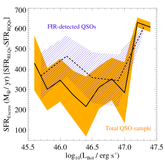
Figure 11: SFR excess between RLQs and RQQs as a function of bolometric luminosity for the total QSO sample (orange) and the FIR detected QSO sample (blue). The solid and dashed lines represent the weighted mean SFR excess and the coloured areas the $1\sigma$ error for the total QSO sample and the FIR detected QSO sample, respectively.

6 Star formation in RG and RLQ

It has been suspected from submillimetre studies that the hosts of powerful radio-loud AGN undergo brief episodes of intense star formation which increase with redshift (e.g. Archibald et al., 2001). Using Herschel data, Seymour et al. (2011) found a mean SFR range of 80 to 600 ${\rm M_{\odot}~{}yr^{-1}}$ for $1.2<z<3.0$ radio-selected AGN. In the same context, Drouart et al. (2014) estimated SFRs of a few hundred to a few thousand solar masses per year for $1<z<5$ radio galaxies. Recently, Podigachoski et al. (2015), comparing the SFR of 3C radio-loud AGN and radio quasars at $z>1$, found similar SFRs for the two classes and at the same levels with the previous works. The idea that the hosts of high-$z$ radio-loud AGN can form stars at high rates is consistent with the jet-induced star formation model.

In this work, while we find that RLQs are associated with vigorous star formation activity, the RGs of this sample have significantly lower SFRs of about a factor of 2.5 for the same BH masses with only two FIR detected sources. Priddey et al. (2003) found quite similar differences (about a factor $\sim 2$) using submillimetre observations of $1.5<z<3$ RQQs and RGs drawn from SCUBA surveys (Archibald et al., 2001). On the other hand, Isaak et al. (2002) suggested that these differences are far less marked at $z>4$.

The FIR-radio luminosity plane is presented in Fig. 8. The RGs in our sample are associated with higher radio luminosities than RLQs (see Fig. 2; almost all RGs have $\log_{10}(L_{325{\rm MHz}}/{\rm W~{}Hz^{-1}~{}sr^{-1}})>26.0$). Assuming that both RGs and RLQs emanate from the same parent population, we find that the FIR luminosities of the most radio luminous sources in Fig. 8 (see RLAGN region) are significantly lower than the radio sources with lower radio luminosities. However, no significant evidence is found regarding an anti-correlation between FIR and radio luminosity.

A possible interpretation of this result would be that star formation enhancement efficiency depends on the radio power, with powerful radio jets associated with negative feedback reducing the star formation in the host galaxy. In fact, radio jet pressure can be sufficiently large to expel significant quantities of gas from the galaxies (Nesvadba et al., 2006), thereby quenching the star formation (Croton et al., 2006). However, this interpretation should also depend on galaxy mass. Indeed, the fraction of radio-loud AGN is a strong function of stellar mass and redshift (e.g. Jiang et al., 2007; Donoso et al., 2009) suggesting that radio jet feedback predominantly occur in massive halos. Thus, we might expect that its influence will have the clearest signature in massive galaxies. Observational studies on this issue return controversial results (e.g. Nesvadba et al., 2010; Papadopoulos et al., 2010) with positive feedback being directly observed in a few local (e.g. Croft et al., 2006), intermediate (e.g. Inskip et al., 2008) and high redshift sources (e.g. Dey et al., 1997; Bicknell et al., 2000). The observed differences could be explained by the fact that galaxy masses vary strongly with redshift but also amongst radio galaxies at similar redshifts (e.g. Kauffmann et al., 2008). In Fig. 8 we compare the SFR between RLQs and RGs with similar radio power (see RLAGN region) and it is clear that RLQs have higher FIR luminosity than RGs. That can be explained as a consequence of the RLQs in the RLAGN region apparently having higher galaxy masses than the RGs (e.g. see Fig. 4 where RLQs are associated with higher black hole masses). Assuming the ${\rm L_{FIR}}-M_{\rm gal}$ relation for $z\sim 1$ as defined by Schreiber et al. (2015) for the RLQs ($\langle M_{\rm gal}\rangle=10^{12.1}~{}M_{\odot}$) and the RGs ($\langle M_{\rm gal}\rangle=10^{11.6}~{}M_{\odot}$) in the RLAGN region we would expect a similar level of FIR luminosity. However, the large uncertainties of the ${\rm L_{FIR}}-M_{\rm gal}$ relation at $M_{\rm gal}>10^{11.5}~{}M_{\odot}$, about $\pm 0.3$ in $\log{\rm L_{FIR}}$, could explain the offset in FIR luminosity we observe in the RLAGN region. This conclusion arises from the assumption that the Magorrian relation holds both ways around.

The RG selection from radio surveys favours objects with the highest values of radio luminosity (i.e. jet power) explaining why the RGs in our sample are more radio luminous than the RLQs. On the other hand, the RLQ selection from both optical and radio surveys favours objects with both high jet power and bolometric luminosity (e.g. accretion rate). However, in all likelihood the quasars are probably biased towards bigger black holes due to the optical selection, as we are selecting on BH properties rather than host galaxy properties.

In order to explain the observed differences regarding the SFR in the two populations taking into account both the galaxy mass and jet power, we suggest a ‘toy model’ in which there is some jet power threshold at which radio-jet feedback switches from enhancing star formation (by compressing gas) to suppressing it (by ejecting gas). Then that threshold will be dependent on both galaxy mass and jet power. In this model, the SFR enhancement (i.e. the level of SFR excess compared to a control sample of radio-quiet AGN with the same bolometric luminosity and galaxy mass) starts from zero for AGN without radio jets, has a mass-dependent peak as jet power increases, and then decreases gradually for higher jet power.

The value of the model is that it can explain the differences between the SFRs estimates in different radio-power sources selected in different ways in recent studies (e.g. Seymour et al., 2011; Dicken et al., 2012; Magliocchetti et al., 2014; Podigachoski et al., 2015; Magliocchetti et al., 2016). It also confirms and extends the high star-forming activity observed in the hosts of radio-active AGN selected by different methods (e.g. Hatziminaoglou et al., 2010; Santini et al., 2012; Rosario et al., 2013; Drouart et al., 2014). For instance, Podigachoski et al. (2015) use a sample of radio-loud objects that is similar in many ways to the dataset in this work, though they target more radio luminous systems. In term of source selection, both Podigachoski et al. (2015) RGs and RLQs samples and our RGs are selected from bright radio surveys (e.g. the Revised Third Cambridge Catalogue of radio sources, hereafter 3CR; Spinrad et al., 1985). Comparing their radio luminosities, the 3CR sample have a $L_{325\rm{MHz}}\geq 10^{26}~{}{\rm W~{}Hz^{-1}~{}sr^{-1}}$ limit which is similar to the one of the radio galaxies in this work (see Fig. 2). Thus, our SFR estimations for the RG population are in perfect agreement ($L_{\rm FIR}\sim 10^{11.7}~{}L_{\odot}$) to the ones found by Podigachoski et al. (2015), especially for their FIR-undetected sample if we consider that almost all of our RGs are FIR-undetected. In addition, our RG systems are also found to have SFRs that are quite similar to inactive galaxies selected from the deeper Herschel surveys (e.g. Rosario et al., 2013). However, this is not the case of the RLQs in this work. As we show in Fig. 2, the RLQs’ radio luminosity goes down to $L_{325\rm{MHz}}\sim 10^{24.5}~{}{\rm W~{}Hz^{-1}~{}sr^{-1}}$ with the majority of the sources having $10^{25}-10^{26}~{}{\rm W~{}Hz^{-1}~{}sr^{-1}}$. As we suggest in our model, at the highest radio powers negative feedback could lead to an overall suppression in SFR. In this case, Podigachoski et al. (2015) results are in agreement with our model as both RGs and RLQs with similar radio luminosities share very similar SFRs, just like the RGs in this work. The fact that our RLQs could be characterized as moderate radio systems, at least compared to the RGs, can possible explain the reported SFRs differences. Apart for the radio-jet positive feedback which could have increased the SFRs in these systems, compared to the RGs and the inactive galaxies, the galaxy mass could also control somehow these results. Specifically, Podigachoski et al. (2015) assume a stellar mass range of $1.5\times 10^{11}-6\times 10^{11}~{}M_{\odot}$. This range is similar to the RGs of our sample (see Fig. 4) but our QSOs extend to higher stellar masses with a mean of $7.5\times 10^{11}~{}M_{\odot}$.

For the same high radio luminosity regime and $z<0.7$, Dicken et al. (2012) did not find a close link between starbursts and powerful radio-loud AGN using Spitzer/Infrared spectroscopy. On the other hand, Magliocchetti et al. (2016) recently found an intense star-forming activity in the majority of less luminous radio-selected AGN ($L_{\rm 1.4~{}GHz}<10^{25}~{}{\rm W~{}HZ^{-1}~{}sr^{-1}}$). A comparison to this work might be hard not only because the different source selection and redshift distribution but also because Magliocchetti et al. (2016) results arise from FIR-detected radio-selected AGN. However, our suggested model seems to be applicable even in this case. Magliocchetti et al. (2016) found that the IR luminosity distribution of their sources peaks at around $L_{\rm IR}=10^{12.5}~{}L_{\odot}$, slightly higher than our mean value for sources with similar stellar mass found in the radio-excess region in Fig. 8.

In order to investigate how our observations fit in this ‘toy model’, we use the RQQs as a control sample. We have separated the RQQs into 4 bolometric luminosity bins, with about the same number of sources ($\sim 18$), and for each bin we estimated the weighted mean specific star-formation rate (sSFR) where the stellar masses are calculated as described in Section 3.1. From low to high bolometric luminosity bins we found $1.472\pm 0.554$, $0.314\pm 0.103$, $0.388\pm 0.089$ and $0.180\pm 0.039~{}{\rm Gyr^{-1}}$. Then, the sSFR of each RLQ and RG in our sample was normalized by the weighted mean sSFR from the RQQ control sample, depending on the bolometric luminosity of each source, in order to estimate the sSFR enchantment fraction associated with the radio jets. We prefer the use of sSFR instead of the SFR in order to account for the galaxy mass dependence in the ‘toy model’. We have excluded six RGs from this analysis with bolometric luminosities lower than the lower RQQ bolometric luminosity bin ($L_{\rm Bol}<10^{45.3}~{}{\rm erg~{}s^{-1}}$, see Fig. 4 middle panel). We note that five of these RGs have been classified as LERGs by Fernandes et al. (2015).

In Fig. 12, we present the fraction of sSFR enhancement due to the radio jets as a function of jet power. As described above, we expect a mass-dependent peak, therefore we normalize the jet power to the Eddington luminosity (i.e. black hole or galaxy mass) in order to control for this dependence. Higher-mass galaxies will be able to hold on to their gas better for a given jet power, so there will be some mass-dependent threshold in jet power beyond which jets tend to have an increasingly suppressing effect on star formation. It seems that our observations follow the suggested ‘toy model’ with sources at the low and intermediate jet power found at the peak of the star-formation enhancement, while at the highest jet power the radio sources have passed the jet power threshold at which radio-jet feedback switches from enhancing star formation to suppressing it. Indeed, the estimated mean sSFR suppresses fraction is $<1$ suggesting that powerful jets for a given galaxy mass suppress the star formation in the host galaxy compared to a radio-quiet source. Larger RG samples, covering a wide range of galaxy masses and radio luminosities, would provide us with additional observational constraints for our model.

Although the suggested model seems to explain the observations, we have to keep in mind that the star formation in the host galaxies of these RLQ and RG systems might be controlled by many additional parameters, like the environment and merger activity, which we expect to be quite common especially for the quasars in our sample (e.g. Santini et al., 2010; Kartaltepe et al., 2012; Ramos Almeida et al., 2012). For instance, Stevens et al. (2003) presented submillimetre imaging of seven high-redshift RGs, several of which present spatially extended massive star-formation activity ($\sim 30-150$ kpc), co-spatial in same cases with similarly extended UV emission (e.g. Hatch et al., 2008). This suggests that the brightest submillimetre companions trace to the high-redshift RGs may trace a large-scale structure which would contain the densest cross-sections of gas. In this case, the very brightest radio sources in our sample, dominated by RGs due to the selection method, might be physically associated with over-dense regions. Therefore, the high jet power sources of our sample might have formed their stars at earlier epochs and we now observe them at a passive evolutionary stage.

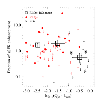
Figure 12: Fraction of sSFR enhancement for RLQs and RGs, normalized to the control sample of RQQs AGN with the same bolometric luminosity, as a function of $Q_{\rm jet}/L_{\rm Edd}$ (jet power over Eddington luminosity). The large black squares are the weighted mean values for the three $Q_{\rm jet}/L_{\rm Edd}$ bins taking into account both RLQs and RGs in each bin. For individual sources, colours and symbols are similar to Fig. 6. FIR undetected sources are presented as upper limits.

7 Conclusions

We have presented Herschel photometry of RLQs, RQQs and RGs selected at a single epoch, $z\approx 1$. Combining the Herschel observations with SMA observations we performed a full radio-FIR SED analysis to investigate the non-thermal contamination to the FIR bands. SDSS data for the QSOs and mid-IR data for the RGs in our sample were used to estimate the AGN luminosity of each source. The FIR observations were used to estimate the SFR for the individually FIR detected sources and the stacked SFR for a variety of AGN and radio properties. We summarize the results below:

1. About 33 per cent (43/149) of the QSOs and 8 per cent (2/27) of the RGs have robust PACS and SPIRE detections. These detection rates are translated to ULIRG-like star formation luminosities suggesting SFRs of hundreds of solar masses per year.

2. SMA 1300 $\mu$m observations lead us to reject 17 RLQs in which the 500 $\mu$m flux may suffer significant synchrotron contamination.

3. We find that about 40 per cent (22/57) of RLQs have robust FIR detections and 30 per cent (21/72) of RQQs. The SFRs of the FIR detected QSOs are higher than a simulated mass-matched galaxy sample supporting the scenario of a merger induced star formation activity. Additionally, the high SFRs and detection rates suggest that there is no clear evidence that the star formation has been quenched in the hosts of these powerful QSOs compared to the non-AGN galaxies. Although radio-jets can enhance the SFR in the RLQs compared to the RQQs, they are not the likely cause of the star formation as RQQ systems as still found with significantly high star formation activity.

4. The FIR luminosity does not show a strong correlation with the AGN luminosity or the stellar mass for any of the three sub-samples in contrast to what is expected for AGN-dominated systems. The lack of dependence on AGN luminosity might suggest that neither the QSO continuum is the cause of star formation activity in any of the AGN systems we studied in this work. A multi-wavelength SED for the measurement of the bolometric luminosity would improve the uncertainties arise from the $L_{12\mu{\rm m}}$ and $L_{3000}$ use for the $L_{\rm bol}$ calculation and their associated bolometric corrections, in order to confirm our results.

5. The RLQs are found to have a SFR excess of about $300~{}{\rm M_{\odot}~{}yr^{-1}}$ (a factor of 2.5) over RQQs of the same bolometric luminosity, similar to the one suggested from simulations in gas-rich radio-loud AGN (Gaibler et al., 2012).

6. Merger induced star formation activity is a possible mechanism leading to the SFRs obtained for RQQs while radio-jet triggered star formation seems to be the likely cause for the SFR excess in RLQs compare to the AGN luminosity matched RQQ sample. It is expected that RGs’ low detection rates are associated with the radio selection of the sample, suggesting the existence of a jet power threshold below which the radio jets enhance the star formation and above which they suppress the star formation in the host galaxy by ejecting gas.

Appendix A Catalogues of the AGN sample and SEDs of the RLQs

In this appendix the best-fit radio to FIR SED plots for a representative sample of RLQs are reported (Fig. 13). Table 2 lists the Herschel photometry of the objects studied in this work with their $1\sigma$ photometric uncertainties (cols. 7, 8, 10, 11, 12) obtained as described in Sec. 2.2. Their PACS and SPIRE observation IDs are given in cols. 6 and 9 indicating also the cases that the observations obtained from public data.

We also present the properties of the total AGN sample in Table 3. The latter lists the following information for each source: right ascension and declination (J2000.0) in degrees (cols. 1 and 2), type classification (col. 3), redshift (col. 4), logarithmic bolometric luminosity measured as described in Sec. 3.2 with the associated $1\sigma$ uncertainty (col. 5), logarithmic 325 MHz radio luminosity including the upper limit estimates for RQQs (col. 6), synchrotron contamination at the FIR bands (Y: for sources with contamination that have been rejected from the sample; col. 7), logarithmic black hole mass measured as described in Sec. 3 with the associated $1\sigma$ uncertainty (col. 8), logarithmic ${\rm L_{FIR}}$ luminosity measured as described in Sec. 3.5 with the associated $1\sigma$ uncertainty (col. 9).

In Table 4 we present the SMA observations of the 44 RLQs candidates for synchrotron contamination. The following information are given for each RLQs: right ascension and declination (J2000.0) in degrees (cols. 1 and 2), atmosheric opacity (col. 3), date of observations (year, month, day; col. 4), observed frequency (col. 5), number of antennas used (col. 6), 1300 $\mu$m flux with the $1\sigma$ error (col. 7). For undetected sources we provide a $4\sigma$ upper limit. Note that for seven sources there are multiple observations due to the poor weather conditions.

Table 2: Table A1. Herschel photometry of the objects studied in this work. Photometric uncertainties are $1\sigma$ values.

name	RA	DEC	type	$z$	PACS_ID	$S_{70\mu{\rm m}}$	$S_{160\mu{\rm m}}$	SPIRE_ID	$S_{250\mu{\rm m}}$	$S_{350\mu{\rm m}}$	$S_{500\mu{\rm m}}$
	(deg)	(deg)				(mJy)	(mJy)		(mJy)	(mJy)	(mJy)
3C356	261.0790	50.9612	RG	1.079	…	…	…	1342206197	$12.21\pm 5.97$	$20.31\pm 5.01$	$-4.02\pm 7.73$
5C7.23	123.4110	29.2749	RG	1.098	1342230090	$0.40\pm 1.90$	$0.57\pm 4.31$	1342244174	$4.45\pm 5.80$	$3.73\pm 5.22$	$7.36\pm 8.26$
5C7.17	123.2474	26.8626	RG	0.936	1342232054	$-0.02\pm 1.79$	$0.58\pm 4.37$	1342230764	$4.03\pm 6.21$	$0.30\pm 5.22$	$6.92\pm 7.00$
3C268.1	180.0995	73.0124	RG	0.970	1342245706	$2.88\pm 1.95$	$1.30\pm 3.57$	1342229628	$2.78\pm 5.97$	$16.03\pm 5.09$	$8.49\pm 7.34$
3C184	114.8511	70.3864	RG	0.994	1342243742	$6.49\pm 1.99$	$17.97\pm 3.64$	1342229126	$19.05\pm 6.21$	$7.95\pm 5.92$	$14.73\pm 7.73$
3C175.1	108.5196	14.6063	RG	0.920	1342242694	$2.77\pm 2.18$	$9.15\pm 4.93$	1342230780	$-2.23\pm 9.00$	$3.87\pm 7.19$	$6.05\pm 10.02$
3C22	12.7343	51.2010	RG	0.936	1342237866	$15.26\pm 2.41$	$15.80\pm 5.38$	…	-99.99	-99.99	-99.99
TOOT1267	3.8791	36.2047	RG	0.968	1342237852	$1.73\pm 1.96$	$5.76\pm 3.92$	1342236247	$10.84\pm 6.26$	$20.63\pm 5.82$	$24.40\pm 7.24$
5C6.24	32.5699	32.8261	RG	1.073	1342237392	$1.82\pm 1.66$	$4.22\pm 3.57$	1342238261	$5.69\pm 6.44$	$-5.20\pm 5.05$	$13.53\pm 8.07$
6C0128+394	22.8731	39.7159	RG	0.929	1342236669	$2.25\pm 1.65$	$4.56\pm 4.13$	1342238258	$-0.43\pm 7.29$	$10.57\pm 6.62$	$26.98\pm 8.70$
3C343	248.6412	62.7601	RG	0.988	1342234218	$34.10\pm 2.32$	$39.63\pm 5.51$	…	-99.99	-99.99	-99.99
3C289	206.3631	49.7754	RG	0.967	1342233495	$6.16\pm 2.01$	$8.60\pm 3.64$	1342232711	$19.62\pm 7.46$	$7.16\pm 5.98$	$0.94\pm 7.93$
3C280	194.2408	47.3389	RG	0.996	1342233434	$11.18\pm 1.99$	$10.96\pm 3.62$	1342232704	$10.55\pm 6.07$	$11.69\pm 4.58$	$13.23\pm 7.20$
6CE1257+3633	194.8753	36.2842	RG	1.004	1342232454	$2.71\pm 1.89$	$2.35\pm 4.66$	1342234906	$9.93\pm 6.052$	$9.76\pm 5.15$	$7.27\pm 6.73$
6CE1017+3712	155.1669	36.9507	RG	1.053	1342232207	$2.32\pm 1.92$	$6.50\pm 4.37$	1342231354	$-1.72\pm 6.52$	$8.13\pm 4.78$	$6.40\pm 7.30$
6CE1011+3632	153.5536	36.2882	RG	1.042	1342231232	$2.53\pm 2.01$	$5.56\pm 3.62$	1342231353	$10.10\pm 6.61$	$26.13\pm 5.81$	$16.41\pm 7.55$
5C7.242	126.4281	24.6725	RG	0.992	1342230085	$7.63\pm 1.58$	$28.75\pm 4.29$	1342230775	$24.60\pm 8.45$	$4.03\pm 7.76$	$-3.27\pm 9.56$
6CE1256+3648	194.7750	36.5326	RG	1.070	1342224630	$4.11\pm 2.05$	$8.14\pm 4.31$	1342234907	$28.48\pm 6.30$	$31.19\pm 5.48$	$15.12\pm 7.12$
6CE1217+3645	185.0410	36.4853	RG	1.088	1342223901	$1.59\pm 1.88$	$11.34\pm 3.94$	1342223250	$17.72\pm 6.85$	$34.98\pm 5.43$	$33.30\pm 7.04$
6CE1129+3710	173.1478	36.9047	RG	1.060	1342222684	$7.28\pm 1.79$	$10.55\pm 3.92$	1342222668	$23.46\pm 7.22$	$32.74\pm 6.35$	$22.52\pm 8.52$
TOOT1140	2.1284	36.3636	RG	0.911	1342237854	$2.23\pm 1.78$	$5.35\pm 3.93$	1342234678	$-4.38\pm 6.46$	$4.58\pm 5.62$	$3.79\pm 6.22$
TOOT1066	3.4510	34.9493	RG	0.926	1342237850	$2.49\pm 1.79$	$6.32\pm 3.76$	1342234679	$10.15\pm 6.38$	$10.13\pm 5.36$	$4.33\pm 7.58$
6C0133+486	24.1693	48.8734	RG	1.029	1342237170	$2.06\pm 2.01$	$9.42\pm 3.76$	1342238257	$-2.21\pm 10.53$	$6.13\pm 10.04$	$-3.13\pm 13.06$
6CE1212+3805	183.7362	37.8141	RG	0.950	1342233115	$2.26\pm 1.85$	$8.87\pm 3.97$	1342223249	$3.85\pm 5.97$	$3.93\pm 5.34$	$4.64\pm 6.31$
6CE0943+3958	146.5779	39.7384	RG	1.035	1342232389	$3.85\pm 1.75$	$5.64\pm 4.24$	1342246616	$6.78\pm 6.32$	$7.26\pm 5.43$	$8.45\pm 6.31$
6CE1019+3924	155.7302	39.1470	RG	0.923	1342231143	$1.66\pm 2.12$	$11.01\pm 4.48$	1342231355	$4.94\pm 6.32$	$18.77\pm 4.87$	$25.78\pm 6.98$
5C7.82	124.4454	29.3640	RG	0.918	1342230088	$2.90\pm 1.95$	$6.58\pm 3.92$	1342230762	$8.72\pm 6.55$	$4.81\pm 5.01$	$0.53\pm 6.48$
SDSS100906.4+023555.3	152.2764	2.5987	RQQ	1.100	1342247311	$2.72\pm 2.71$	$4.24\pm 2.65$	??	$21.46\pm 6.24$	$9.63\pm 4.04$	$5.42\pm 7.89$
SDSS100730.5+050942.3	151.8770	5.1617	RQQ	0.920	1342254150	$13.32\pm 2.19$	$56.86\pm 5.37$	1342246597	$68.67\pm 6.36$	$40.09\pm 5.40$	$8.79\pm 5.13$
SDSS103347.3+094039.0	158.4471	9.6775	RQQ	1.028	1342246737	$13.46\pm 2.71$	$19.63\pm 5.01$	1342222671	$31.29\pm 5.98$	$25.15\pm 5.21$	$19.31\pm 7.58$
SDSS102006.0+033308.5	155.0249	3.5523	RQQ	0.936	1342246735	$8.33\pm 2.70$	$13.11\pm 5.09$	1342247237	$19.08\pm 6.16$	$19.84\pm 4.98$	$16.93\pm 6.59$
SDSS094811.9+551726.5	147.0494	55.2917	RQQ	1.034	1342246701	$3.62\pm 3.14$	$7.10\pm 5.26$	1342229498	$14.23\pm 6.01$	$14.44\pm 5.09$	$1.56\pm 6.79$
SDSS104659.4+573055.6	161.7474	57.5155	RQQ	1.026	1342246198	$3.22\pm 2.46$	$5.43\pm 5.60$	??	$5.75\pm 6.84$	$9.47\pm 5.74$	$11.47\pm 6.46$
SDSS093759.4+542427.3	144.4973	54.4076	RQQ	1.067	1342246196	$6.48\pm 2.51$	$19.99\pm 5.29$	1342229496	$62.29\pm 6.18$	$80.68\pm 5.31$	$70.17\pm 8.41$
SDSS104930.5+592032.6	162.3769	59.3424	RQQ	1.011	1342245702	$8.92\pm 3.43$	$12.72\pm 4.65$	L-SWIREα	$10.05\pm 6.21$	$6.16\pm 5.09$	$4.69\pm 7.38$
SDSS104859.7+565648.6	162.2486	56.9468	RQQ	1.014	1342245700	$6.24\pm 2.99$	$17.40\pm 5.49$	L-SWIREα	$13.01\pm 6.27$	$25.35\pm 5.09$	$14.18\pm 6.26$
SDSS104239.7+583231.0	160.6652	58.5420	RQQ	0.998	1342245698	$3.46\pm 2.51$	$8.95\pm 5.63$	L-SWIREα	$14.02\pm 6.16$	$10.87\pm 5.40$	$10.09\pm 7.48$
SDSS104355.5+593054.0	160.9811	59.5150	RQQ	0.909	1342245696	$4.22\pm 2.38$	$19.64\pm 5.42$	L-SWIREα	$15.55\pm 6.24$	$13.50\pm 4.18$	$8.73\pm 7.58$
SDSS091216.9+420314.2	138.0703	42.0540	RQQ	1.077	1342245680	$2.82\pm 2.65$	$14.20\pm 4.67$	1342230744	$10.48\pm 6.95$	$16.83\pm 5.32$	$-0.70\pm 7.25$
SDSS092257.9+444651.8	140.7411	44.7811	RQQ	1.077	1342245678	$12.29\pm 2.74$	$29.01\pm 5.75$	1342230742	$32.54\pm 5.76$	$33.80\pm 5.36$	$12.81\pm 7.30$

A1. continued

name	RA	DEC	type	z	PACS_ID	$S_{70\mu{\rm m}}$	$S_{160\mu{\rm m}}$	SPIRE_ID	$S_{250\mu{\rm m}}$	$S_{350\mu{\rm m}}$	$S_{500\mu{\rm m}}$
	(deg)	(deg)				(mJy)	(mJy)		(mJy)	(mJy)	(mJy)
SDSS093303.5+460440.2	143.2645	46.0777	RQQ	1.090	1342245676	$6.26\pm 2.33$	$15.88\pm 4.86$	1342230741	$22.10\pm 6.16$	$19.78\pm 5.43$	$14.35\pm 7.75$
SDSS104114.2+590219.4	160.3091	59.0387	RQQ	1.094	1342245196	$4.17\pm 2.72$	$5.99\pm 5.44$	L-SWIREα	$10.06\pm 5.95$	$4.77\pm 5.75$	$2.85\pm 8.24$
SDSS103829.7+585204.1	159.6239	58.8678	RQQ	0.935	1342245194	$6.99\pm 2.85$	$17.26\pm 5.83$	L-SWIREα	$32.41\pm 6.17$	$22.88\pm 5.21$	$16.10\pm 6.88$
SDSS090153.4+065915.6	135.4726	6.9876	RQQ	1.082	1342245188	$7.61\pm 2.49$	$15.07\pm 4.77$	1342230785	$25.98\pm 6.50$	$31.90\pm 5.55$	$25.57\pm 7.58$
SDSS084723.7+011010.4	131.8485	1.1695	RQQ	1.081	1342244276	$3.75\pm 2.30$	$13.86\pm 5.74$	H-ATLASb	$17.24\pm 7.69$	$18.07\pm 5.11$	$5.80\pm 7.17$
SDSS074729.2+434607.5	116.8715	43.7688	RQQ	1.086	1342243754	$3.46\pm 2.56$	$8.21\pm 4.76$	1342229647	$-1.70\pm 6.36$	$10.25\pm 5.11$	$6.73\pm 6.26$
SDSS082229.8+442705.2	125.6240	44.4515	RQQ	1.057	1342243308	$8.99\pm 2.39$	$4.73\pm 5.81$	1342229484	$0.93\pm 7.02$	$-7.16\pm 8.04$	$4.60\pm 8.30$
SDSS083115.9+423316.6	127.8161	42.5546	RQQ	0.931	1342243304	$16.87\pm 2.54$	$48.53\pm 5.45$	1342229482	$58.69\pm 5.52$	$39.14\pm 5.66$	$10.96\pm 6.96$
SDSS075058.2+421617.0	117.7425	42.2714	RQQ	0.938	1342243241	$2.84\pm 2.28$	$5.62\pm 4.98$	1342229648	$3.24\pm 6.45$	$16.42\pm 4.90$	$15.45\pm 6.46$
SDSS115027.3+665848.0	177.6134	66.9800	RQQ	1.035	1342243213	$11.34\pm 2.37$	$9.22\pm 4.76$	1342229501	$15.84\pm 5.04$	$13.73\pm 4.18$	$4.91\pm 5.13$
SDSS171704.7+281400.6	259.2695	28.2335	RQQ	1.078	1342241359	$36.59\pm 2.57$	$44.26\pm 4.02$	1342229587	$42.86\pm 7.38$	$35.24\pm 6.31$	$25.47\pm 7.24$
SDSS023540.9+001038.9	38.92043	0.1775	RQQ	0.948	1342238857	$4.81\pm 2.34$	$18.20\pm 4.93$	1342238276	$6.97\pm 7.01$	$-5.50\pm 5.70$	$0.31\pm 9.06$
SDSS145503.5+014209.0	223.7644	1.7025	RQQ	1.053	1342237890	$4.36\pm 2.42$	$21.94\pm 5.40$	1342238316	$40.95\pm 6.08$	$56.54\pm 5.61$	$21.51\pm 7.84$
SDSS151520.6+004739.3	228.8356	0.7943	RQQ	0.951	1342237144	$14.47\pm 2.39$	$36.68\pm 5.46$	1342238313	$52.51\pm 6.84$	$39.97\pm 6.24$	$25.63\pm 8.90$
SDSS135824.0+021343.8	209.5999	2.2289	RQQ	0.957	1342236962	$8.16\pm 2.49$	$8.46\pm 5.02$	1342236164	$6.67\pm 6.02$	$-0.39\pm 5.21$	$-1.09\pm 6.63$
SDSS224159.4+142055.2	340.4976	14.3486	RQQ	0.954	1342235592	$5.88\pm 2.35$	$9.44\pm 4.95$	1342220640	$15.76\pm 5.87$	$14.30\pm 5.22$	$8.04\pm 5.80$
SDSS155436.3+320408.4	238.6510	32.0690	RQQ	1.058	1342235402	$5.58\pm 2.37$	$11.47\pm 5.87$	1342229550	$23.63\pm 6.06$	$24.20\pm 5.04$	$13.01\pm 7.59$
SDSS134635.0+415630.9	206.6459	41.9419	RQQ	0.902	1342235358	$2.53\pm 2.71$	$34.53\pm 5.87$	1342232713	$22.18\pm 5.97$	$53.14\pm 4.90$	$24.57\pm 7.89$
SDSS145506.1+562935.6	223.7754	56.4932	RQQ	1.039	1342235348	$9.66\pm 2.76$	$25.06\pm 5.97$	1342227745	$19.20\pm 5.89$	$24.28\pm 4.99$	$7.83\pm 5.55$
SDSS171145.5+601318.4	257.9397	60.2218	RQQ	0.980	1342235342	$3.72\pm 2.44$	$5.45\pm 5.59$	FLSc	$8.08\pm 6.32$	$12.25\pm 6.31$	$15.06\pm 7.58$
SDSS171732.9+594747.7	259.3872	59.7965	RQQ	1.060	1342235340	$7.39\pm 2.55$	$17.06\pm 5.12$	FLSc	$27.74\pm 6.24$	$25.23\pm 5.22$	$9.22\pm 6.61$
SDSS172310.4+595105.6	260.7931	59.8516	RQQ	0.990	1342235338	$7.41\pm 2.64$	$22.65\pm 5.29$	FLSc	$30.39\pm 6.17$	$20.15\pm 5.22$	$12.11\pm 7.01$
SDSS171005.5+644843.0	257.5230	64.8119	RQQ	1.008	1342235336	$21.71\pm 2.52$	$65.92\pm 5.41$	1342229143	$94.70\pm 6.11$	$76.58\pm 4.97$	$46.75\pm 7.21$
SDSS171330.2+644253.0	258.3760	64.7147	RQQ	1.051	1342235334	$17.80\pm 2.25$	$34.04\pm 6.02$	1342229142	$42.70\pm 5.60$	$22.93\pm 4.39$	$9.25\pm 6.06$
SDSS215541.7+122818.8	328.9239	12.4719	RQQ	1.064	1342234438	$8.49\pm 2.47$	$16.42\pm 5.54$	1342233328	$15.40\pm 7.34$	$3.75\pm 6.25$	$-1.47\pm 7.63$
SDSS142817.3+502712.6	217.0721	50.4535	RQQ	1.013	1342234359	$11.72\pm 2.43$	$10.58\pm 5.46$	1342232718	$7.86\pm 6.24$	$12.87\pm 4.99$	$3.70\pm 7.71$
SDSS155650.4+394542.8	239.2100	39.7619	RQQ	0.942	1342234355	$16.32\pm 2.63$	$70.04\pm 5.07$	1342229546	$70.57\pm 6.21$	$64.89\pm 5.62$	$23.46\pm 7.05$
SDSS151921.9+535842.3	229.8410	53.9784	RQQ	1.027	1342234220	$2.91\pm 2.63$	$4.91\pm 4.44$	1342229522	$2.98\pm 6.50$	$0.86\pm 5.88$	$-2.00\pm 6.36$
SDSS163225.6+411852.0	248.1065	41.3146	RQQ	0.909	1342234078	$6.04\pm 2.63$	$12.29\pm 5.58$	ELAIS-N2d	$12.62\pm 6.54$	$16.48\pm 4.88$	$8.54\pm 7.53$
SDSS163306.1+401747.0	248.2755	40.2965	RQQ	0.974	1342234076	$5.10\pm 2.49$	$9.30\pm 5.69$	ELAIS-N2d	$19.34\pm 5.87$	$28.82\pm 6.24$	$15.34\pm 6.21$
SDSS163930.8+410013.2	249.8784	41.0038	RQQ	1.052	1342234074	$2.67\pm 2.44$	$8.79\pm 5.71$	ELAIS-N2d	$13.36\pm 6.52$	$10.93\pm 6.25$	$3.52\pm 5.95$
SDSS142124.7+423003.2	215.3528	42.5009	RQQ	1.001	1342233511	$9.86\pm 2.43$	$21.44\pm 5.99$	1342236137	$31.63\pm 6.17$	$38.37\pm 5.02$	$31.02\pm 7.24$
SDSS132957.2+540505.9	202.4881	54.0850	RQQ	0.949	1342233436	$27.86\pm 2.78$	$19.38\pm 5.11$	1342230863	$21.14\pm 6.27$	$1.71\pm 5.41$	$3.25\pm 7.0$
SDSS104935.8+554950.6	162.3990	55.8307	RQQ	1.056	1342233424	$6.06\pm 2.56$	$9.72\pm 5.22$	L-SWIREα	$14.35\pm 6.24$	$19.98\pm 5.43$	$25.09\pm 6.88$
SDSS104537.7+484914.6	161.4070	48.8207	RQQ	0.943	1342233418	$2.20\pm 2.47$	$18.13\pm 5.46$	1342222656	$19.36\pm 5.93$	$29.38\pm 4.95$	$12.71\pm 5.95$
SDSS092753.5+053637.0	141.9730	5.61023	RQQ	1.062	1342233406	$8.83\pm 2.31$	$21.11\pm 5.67$	1342245557	$12.90\pm 7.69$	$9.53\pm 6.29$	$16.33\pm 9.04$
SDSS100835.8+513927.8	152.1493	51.6577	RQQ	1.085	1342232405	$5.60\pm 2.50$	$12.09\pm 5.13$	1342221914	$11.92\pm 5.95$	$7.95\pm 4.88$	$8.23\pm 7.01$

A1. continued

name	RA	DEC	type	z	PACS_ID	$S_{70\mu{\rm m}}$	$S_{160\mu{\rm m}}$	SPIRE_ID	$S_{250\mu{\rm m}}$	$S_{350\mu{\rm m}}$	$S_{500\mu{\rm m}}$
	(deg)	(deg)				(mJy)	(mJy)		(mJy)	(mJy)	(mJy)
SDSS092829.9+504836.6	142.1241	50.8101	RQQ	1.034	1342232401	$2.42\pm 2.73$	$8.72\pm 5.31$	1342230874	$-5.27\pm 6.54$	$5.71\pm 5.22$	$0.72\pm 7.48$
SDSS133733.3+590622.6	204.3887	59.1063	RQQ	1.087	1342232192	$16.15\pm 2.23$	$14.01\pm 6.31$	1342229512	$25.71\pm 5.81$	$22.39\pm 5.00$	$18.97\pm 6.72$
SDSS133713.1+610749.0	204.3042	61.1303	RQQ	0.926	1342232190	$3.07\pm 2.33$	$6.44\pm 6.01$	1342229510	$7.20\pm 6.54$	$7.40\pm 5.14$	$6.86\pm 8.04$
SDSS122832.9+603735.1	187.1372	60.6264	RQQ	1.040	1342232184	$2.48\pm 2.51$	$6.13\pm 5.84$	1342229504	$6.62\pm 5.34$	$9.46\pm 4.87$	$5.73\pm 6.88$
SDSS093023.3+403111.0	142.5970	40.5197	RQQ	1.097	1342232034	$6.05\pm 2.49$	$19.05\pm 5.20$	1342230747	$21.71\pm 6.58$	$11.73\pm 5.27$	$9.06\pm 6.59$
SDSS073802.4+383116.3	114.5098	38.5213	RQQ	1.023	1342231556	$35.02\pm 2.46$	$64.91\pm 4.67$	1342229479	$104.45\pm 6.32$	$70.82\pm 5.15$	$32.79\pm 7.39$
SDSS075339.8+250137.9	118.4159	25.0272	RQQ	0.943	1342230047	$6.87\pm 2.34$	$11.16\pm 5.18$	1342229469	$6.36\pm 8.84$	$15.31\pm 7.30$	$3.41\pm 8.58$
SDSS075222.9+273823.2	118.0954	27.6397	RQQ	1.057	1342230045	$20.85\pm 2.65$	$14.18\pm 5.32$	1342229471	$8.92\pm 6.17$	$1.09\pm 4.97$	$3.79\pm 7.17$
SDSS003146.1+134629.6	7.941963	13.7750	RQQ	1.007	1342225481	$2.20\pm 2.63$	$7.85\pm 4.09$	1342234686	$8.45\pm 5.95$	$3.82\pm 4.98$	$-0.53\pm 7.38$
SDSS164617.2+364509.4	251.5715	36.7527	RQQ	0.958	1342225443	$3.54\pm 2.29$	$9.45\pm 5.31$	1342229595	$19.12\pm 6.23$	$29.14\pm 4.94$	$14.10\pm 6.96$
SDSS165231.3+353615.9	253.1304	35.6044	RQQ	0.928	1342225441	$4.46\pm 2.46$	$22.62\pm 5.74$	1342229596	$32.60\pm 6.32$	$26.42\pm 5.74$	$6.55\pm 7.01$
SDSS163408.6+331242.1	248.5360	33.2117	RQQ	1.007	1342225437	$4.19\pm 2.59$	$5.39\pm 5.18$	1342229593	$11.83\pm 6.36$	$11.02\pm 5.52$	$-3.61\pm 6.90$
SDSS125659.9+042734.4	194.2496	4.4596	RQQ	1.025	1342224527	$53.24\pm 2.51$	$57.65\pm 5.86$	1342234887	$65.53\pm 6.46$	$42.30\pm 5.40$	$21.01\pm 7.01$
SDSS123059.7+101624.8	187.7488	10.2735	RQQ	1.056	1342223937	$1.72\pm 2.31$	$3.94\pm 4.76$	1342187266	$18.87\pm 6.32$	$7.82\pm 6.31$	$6.15\pm 5.13$
SDSS112317.5+051804.0	170.8229	5.3011	RQQ	1.000	1342223674	$20.88\pm 2.60$	$16.75\pm 5.01$	1342222902	$18.03\pm 6.32$	$4.87\pm 5.91$	$2.25\pm 8.24$
SDSS105408.9+042650.4	163.5370	4.4473	RQQ	1.085	1342223306	$9.20\pm 2.14$	$35.22\pm 5.62$	1342234865	$38.59\pm 5.44$	$34.75\pm 4.78$	$17.26\pm 6.21$
SDSS172131.0+584404.1	260.3790	58.7347	RQQ	1.000	1342223190	$2.58\pm 2.57$	$22.47\pm 5.13$	FLSc	$15.31\pm 5.44$	$15.24\pm 5.02$	$15.40\pm 6.70$
SDSS114700.4+620008.1	176.7515	62.0023	RQQ	1.041	1342222698	$22.19\pm 2.32$	$47.16\pm 5.08$	1342229502	$68.20\pm 6.85$	$43.16\pm 5.80$	$18.97\pm 7.53$
SDSS102111.6+611415.0	155.2982	61.2376	RQQ	0.931	1342222523	$2.94\pm 2.42$	$5.48\pm 5.05$	1342229500	$10.44\pm 6.02$	$-1.69\pm 5.75$	$3.01\pm 6.70$
SDSS103525.1+580335.6	158.8544	58.0599	RQQ	0.964	1342222521	$2.78\pm 2.28$	$11.10\pm 5.12$	L-SWIREα	$22.24\pm 5.89$	$15.64\pm 5.22$	$6.55\pm 7.17$
SDSS103855.3+575814.7	159.7305	57.9708	RQQ	0.956	1342222519	$4.77\pm 2.49$	$11.32\pm 5.06$	L-SWIREα	$14.15\pm 5.04$	$12.82\pm 4.88$	$9.87\pm 7.01$
SDSS102349.4+522151.2	155.9558	52.3642	RQQ	0.955	1342222517	$9.41\pm 5.63$	$21.14\pm 5.63$	1342230877	$42.85\pm 6.52$	$36.92\pm 5.74$	$13.39\pm 6.61$
SDSS160913.2+535429.6	242.3049	53.9082	RLQ	0.992	ELAIS-N1	$<2.36$	$<5.67$	ELAIS-N1	$8.58\pm 6.37$	$7.23\pm 4.40$	$6.10\pm 6.21$
SDSS074417.5+375317.2	116.0728	37.8881	RLQ	1.067	1342206178	$<2.29$	$<4.75$	1342206178	$17.78\pm 6.05$	$15.10\pm 4.42$	$12.78\pm 6.75$
SDSS100940.5+465525.0	152.4185	46.9236	RLQ	1.013	1342254137	$5.01\pm 2.45$	$8.58\pm 5.14$	1342231356	$4.15\pm 6.19$	$0.19\pm 4.72$	$-0.22\pm 6.46$
SDSS094740.0+515456.8	146.9162	51.9158	RLQ	1.063	1342246699	$2.41\pm 2.48$	$5.72\pm 4.62$	1342230875	$7.47\pm 5.86$	$6.09\pm 4.83$	$5.01\pm 6.11$
SDSS100943.6+052953.9	152.4314	5.4983	RLQ	0.942	1342246211	$7.87\pm 2.39$	$1.74\pm 5.67$	1342247238	$98.14\pm 6.38$	$97.96\pm 5.18$	$58.81\pm 6.86$
SDSS104156.5+593611.2	160.4855	59.6031	RLQ	1.100	1342245198	$7.08\pm 2.69$	$8.73\pm 6.13$	L-SWIREα	$15.75\pm 6.19$	$11.03\pm 4.75$	$11.09\pm 7.19$
SDSS084028.3+323229.4	130.1180	32.5415	RLQ	1.099	1342244258	$3.13\pm 2.26$	$10.75\pm 5.36$	1342230760	$20.06\pm 6.05$	$23.70\pm 5.31$	$14.84\pm 6.93$
SDSS090142.4+425631.0	135.4266	42.9419	RLQ	1.014	1342244252	$3.14\pm 2.46$	$11.27\pm 5.11$	1342244173	$12.16\pm 6.19$	$32.11\pm 5.53$	$23.64\pm 7.86$
SDSS083110.0+374209.6	127.7917	37.7026	RLQ	0.919	1342243810	$10.14\pm 2.18$	$17.16\pm 5.45$	1342230754	$25.97\pm 5.72$	$28.99\pm 5.33$	$24.61\pm 7.02$
SDSS082901.3+371806.1	127.2553	37.3017	RLQ	0.934	1342243808	$8.66\pm 2.44$	$64.38\pm 5.35$	1342229480	$120.24\pm 6.41$	$92.21\pm 5.30$	$47.75\pm 7.84$
SDSS083226.1+343414.3	128.1087	34.5708	RLQ	1.005	1342243806	$3.72\pm 2.30$	$8.81\pm 4.98$	1342230756	$18.93\pm 6.63$	$24.49\pm 5.40$	$14.55\pm 7.74$
SDSS083315.1+350647.3	128.3128	35.1131	RLQ	1.098	1342243804	$4.52\pm 2.59$	$7.70\pm 4.55$	1342230753	$4.76\pm 6.26$	$-1.69\pm 5.18$	$2.41\pm 7.47$
SDSS083407.6+354712.0	128.5315	35.7867	RLQ	1.088	1342243802	$2.22\pm 2.54$	$19.09\pm 5.55$	1342230752	$17.01\pm 6.66$	$25.94\pm 5.78$	$7.49\pm 8.08$
SDSS090037.9+550318.0	135.1578	55.0550	RLQ	0.947	1342243324	$17.93\pm 2.70$	$38.40\pm 5.85$	1342229493	$40.07\pm 5.96$	$29.30\pm 4.77$	$11.56\pm 6.46$
SDSS083248.4+422459.5	128.2018	42.4165	RLQ	1.051	1342243306	$3.77\pm 2.64$	$12.31\pm 5.73$	1342229481	$4.42\pm 5.95$	$11.47\pm 5.01$	$11.93\pm 7.43$
SDSS082012.6+431358.5	125.0526	43.2329	RLQ	1.073	1342243239	$3.50\pm 2.70$	$13.22\pm 4.60$	1342229483	$8.54\pm 5.98$	$18.57\pm 5.51$	$6.62\pm 7.19$
SDSS082836.4+504826.5	127.1515	50.8074	RLQ	0.929	1342243233	$2.92\pm 2.58$	$12.38\pm 5.64$	1342229487	$30.16\pm 6.63$	$46.69\pm 5.87$	$49.11\pm 7.55$
SDSS150759.1+020053.8	226.9960	2.0150	RLQ	1.083	1342236618	$59.30\pm 2.50$	$117.75\pm 5.92$	1342238315	$135.04\pm 6.37$	$76.86\pm 5.66$	$34.08\pm 7.81$
SDSS163625.0+361458.0	249.1042	36.2494	RLQ	0.909	1342235406	$4.56\pm 2.44$	$31.22\pm 5.62$	1342229594	$40.20\pm 6.34$	$31.22\pm 5.26$	$15.25\pm 7.44$

A1. continued

name	RA	DEC	type	z	PACS_ID	$S_{70\mu{\rm m}}$	$S_{160\mu{\rm m}}$	SPIRE_ID	$S_{250\mu{\rm m}}$	$S_{350\mu{\rm m}}$	$S_{500\mu{\rm m}}$
	(deg)	(deg)				(mJy)	(mJy)		(mJy)	(mJy)	(mJy)
SDSS160516.1+313620.8	241.3169	31.6058	RLQ	1.028	1342235404	$3.85\pm 2.41$	$11.00\pm 5.12$	1342229552	$1.44\pm 5.91$	$-5.59\pm 5.26$	$-8.40\pm 6.80$
SDSS152949.8+394509.6	232.4573	39.7527	RLQ	1.081	1342235396	$3.11\pm 2.76$	$13.69\pm 5.32$	1342229534	$12.02\pm 6.03$	$4.28\pm 4.51$	$2.03\pm 6.88$
SDSS155729.9+330446.9	239.3747	33.0797	RLQ	0.954	1342235114	$3.83\pm 2.64$	$2.79\pm 5.05$	1342229549	$24.43\pm 6.43$	$63.98\pm 6.05$	$69.34\pm 7.35$
SDSS163403.0+390000.6	248.5125	39.0002	RLQ	1.085	1342234446	$6.02\pm 2.47$	$18.73\pm 5.22$	1342229542	$31.54\pm 5.99$	$20.44\pm 4.69$	$18.76\pm 7.21$
SDSS150031.8+483646.8	225.1323	48.6131	RLQ	1.028	1342234357	$23.01\pm 2.88$	$36.41\pm 5.72$	1342229521	$42.58\pm 6.68$	$36.67\pm 6.10$	$14.00\pm 6.86$
SDSS161806.3+422532.1	244.5264	42.4256	RLQ	0.934	1342234347	$7.11\pm 2.75$	$5.10\pm 5.09$	1342229545	$9.33\pm 6.12$	$-0.62\pm 5.07$	$5.11\pm 6.75$
SDSS162553.3+434713.8	246.4721	43.7872	RLQ	1.048	1342234250	$22.14\pm 2.71$	$62.71\pm 5.43$	1342229539	$102.43\pm 7.00$	$81.10\pm 5.73$	$53.42\pm 6.91$
SDSS162917.8+443452.4	247.3241	44.5812	RLQ	1.033	1342234248	$4.02\pm 2.88$	$11.08\pm 5.45$	1342229538	$6.13\pm 6.12$	$-0.18\pm 5.36$	$-4.78\pm 6.79$
SDSS161603.8+463225.3	244.0157	46.5404	RLQ	0.950	1342234246	$4.37\pm 2.74$	$11.17\pm 5.56$	1342229537	$18.24\pm 5.90$	$24.93\pm 4.96$	$19.80\pm 6.76$
SDSS144837.5+501448.9	222.1564	50.2469	RLQ	1.074	1342234222	$2.75\pm 3.02$	$17.04\pm 5.24$	1342229520	$27.36\pm 6.24$	$56.42\pm 6.34$	$41.85\pm 8.28$
SDSS121529.6+533555.9	183.8731	53.5989	RLQ	1.069	1342233543	$7.68\pm 2.55$	$9.73\pm 6.09$	1342223240	$7.78\pm 5.80$	$12.07\pm 5.15$	$8.86\pm 6.34$
SDSS141802.8+414935.3	214.5116	41.8265	RLQ	1.042	1342233513	$6.83\pm 2.82$	$81.33\pm 5.96$	1342236138	$90.13\pm 6.15$	$84.86\pm 5.04$	$41.94\pm 6.27$
SDSS142829.9+443949.8	217.1247	44.6638	RLQ	1.050	1342233509	$1.92\pm 2.52$	$8.90\pm 5.54$	1342232722	$11.53\pm 6.46$	$13.96\pm 4.82$	$7.72\pm 7.97$
SDSS143746.6+443258.6	219.4442	44.5496	RLQ	0.944	1342233507	$2.71\pm 2.36$	$10.75\pm 5.05$	1342232724	$25.15\pm 6.09$	$18.51\pm 4.40$	$8.58\pm 6.21$
SDSS143253.7+460343.8	218.2239	46.0622	RLQ	1.077	1342233505	$6.20\pm 2.42$	$12.86\pm 6.04$	1342232721	$12.98\pm 5.39$	$16.37\pm 4.88$	$9.73\pm 6.35$
SDSS141028.2+460821.0	212.6174	46.1391	RLQ	1.016	1342233499	$5.26\pm 2.50$	$11.94\pm 5.99$	1342232716	$21.04\pm 5.60$	$19.23\pm 4.42$	$19.75\pm 5.94$
SDSS133749.6+550102.2	204.4568	55.0174	RLQ	1.099	1342233493	$7.74\pm 2.72$	$19.28\pm 5.06$	1342230862	$38.26\pm 5.53$	$42.74\pm 4.57$	$50.39\pm 6.02$
SDSS134934.6+534117.0	207.3944	53.6881	RLQ	0.979	1342233491	$21.92\pm 2.77$	$40.64\pm 5.75$	1342230861	$52.98\pm 5.50$	$58.65\pm 4.77$	$54.92\pm 7.25$
SDSS134213.3+602142.8	205.5552	60.3619	RLQ	0.965	1342233440	$11.32\pm 2.29$	$26.35\pm 5.73$	1342229511	$37.11\pm 5.53$	$59.46\pm 5.57$	$31.19\pm 6.66$
SDSS131103.2+551354.4	197.7632	55.2317	RLQ	0.925	1342233438	$19.25\pm 2.72$	$49.54\pm 5.86$	1342230864	$70.21\pm 6.25$	$80.84\pm 5.85$	$85.98\pm 7.61$
SDSS122339.3+461118.7	185.9138	46.1886	RLQ	1.013	1342233432	$3.35\pm 2.38$	$6.42\pm 5.50$	1342223244	$21.65\pm 6.51$	$30.05\pm 5.21$	$36.47\pm 7.43$
SDSS112023.2+540427.1	170.0966	54.0742	RLQ	0.923	1342233426	$2.91\pm 2.46$	$5.16\pm 4.68$	1342222660	$-0.65\pm 6.70$	$3.97\pm 5.19$	$14.49\pm 6.80$
SDSS104542.2+525112.6	161.4257	52.8534	RLQ	1.058	1342233420	$10.47\pm 2.25$	$15.84\pm 4.81$	1342222657	$25.06\pm 5.72$	$37.58\pm 5.15$	$25.29\pm 7.19$
SDSS090910.1+012135.7	137.2919	1.35987	RLQ	1.024	1342233404	$28.74\pm 2.50$	$77.85\pm 5.59$	H-ATLASb	$258.11\pm 5.11$	$337.74\pm 4.53$	$424.86\pm 7.84$
SDSS155416.5+513218.9	238.5689	51.5386	RLQ	0.907	1342233362	$5.23\pm 2.36$	$9.87\pm 5.67$	1342229530	$16.02\pm 5.92$	$28.41\pm 5.41$	$10.82\pm 6.92$
SDSS144527.4+392117.0	221.3642	39.3547	RLQ	0.965	1342233210	$2.45\pm 2.50$	$13.82\pm 4.98$	1342236136	$3.71\pm 5.67$	$6.72\pm 5.48$	$2.77\pm 6.19$
SDSS095227.3+504850.7	148.1135	50.8140	RLQ	1.091	1342232403	$2.95\pm 2.47$	$15.12\pm 4.87$	1342246620	$18.82\pm 6.65$	$6.37\pm 6.10$	$3.37\pm 6.91$
SDSS091921.6+504855.4	139.8397	50.8154	RLQ	0.921	1342232399	$4.96\pm 2.45$	$11.55\pm 4.96$	1342229490	$32.99\pm 5.75$	$26.46\pm 4.40$	$19.81\pm 6.43$
SDSS090812.2+514700.8	137.0506	51.7836	RLQ	1.002	1342232397	$2.96\pm 2.35$	$11.32\pm 4.44$	1342229489	$12.24\pm 6.05$	$1.64\pm 5.96$	$-0.70\pm 8.15$
SDSS091011.0+463617.8	137.5459	46.6049	RLQ	1.020	1342232395	$13.48\pm 2.64$	$24.60\pm 4.86$	1342245573	$19.53\pm 6.20$	$20.54\pm 5.33$	$9.92\pm 7.36$
SDSS152556.2+591659.5	231.4844	59.2832	RLQ	0.955	1342232198	$3.12\pm 2.33$	$5.91\pm 3.89$	1342229523	$35.80\pm 5.38$	$33.69\pm 5.76$	$30.21\pm 7.55$
SDSS150133.9+613733.8	225.3912	61.6260	RLQ	0.910	1342232196	$2.76\pm 2.58$	$4.25\pm 4.75$	1342229515	$23.28\pm 6.05$	$18.36\pm 4.89$	$13.26\pm 6.62$
SDSS134357.6+575442.5	205.9898	57.9118	RLQ	0.933	1342232194	$6.02\pm 2.41$	$5.63\pm 5.32$	1342229513	$26.26\pm 6.35$	$42.04\pm 5.68$	$28.75\pm 6.46$
SDSS081520.6+273617.0	123.8360	27.6047	RLQ	0.908	1342232052	$29.36\pm 2.37$	$37.79\pm 5.43$	1342230763	$43.84\pm 5.65$	$28.20\pm 4.89$	$24.79\pm 6.93$
SDSS080915.9+321041.6	122.3161	32.1782	RLQ	0.915	1342232050	$2.81\pm 2.64$	$6.49\pm 4.83$	1342229476	$16.84\pm 6.58$	$20.18\pm 5.19$	$14.23\pm 7.00$
SDSS093332.7+414945.0	143.3862	41.8292	RLQ	0.933	1342232032	$2.64\pm 2.41$	$7.98\pm 4.97$	1342230745	$-0.48\pm 5.96$	$-6.97\pm 4.61$	$3.51\pm 6.82$
SDSS132909.3+480109.7	202.2885	48.0194	RLQ	0.928	1342231664	$3.72\pm 2.44$	$12.36\pm 5.74$	1342232708	$32.45\pm 6.41$	$22.40\pm 5.75$	$19.76\pm 7.41$
SDSS154515.9+432953.1	236.3162	43.4981	RLQ	0.903	1342231247	$5.43\pm 2.51$	$6.62\pm 5.40$	1342229535	$26.11\pm 5.61$	$30.51\pm 5.43$	$19.29\pm 7.61$
SDSS155405.0+461107.5	238.5209	46.1855	RLQ	1.004	1342231245	$3.87\pm 2.60$	$11.54\pm 4.90$	1342229536	$-0.09\pm 6.63$	$11.70\pm 5.84$	$9.96\pm 6.41$
SDSS094644.7+414304.5	146.6864	41.7179	RLQ	1.018	1342231239	$5.59\pm 2.61$	$9.91\pm 5.68$	1342246617	$12.15\pm 6.65$	$-0.02\pm 5.81$	$4.99\pm 7.86$
SDSS163302.1+392427.4	248.2587	39.4076	RLQ	1.024	1342231121	$25.33\pm 2.55$	$21.50\pm 6.14$	1342229541	$14.72\pm 5.41$	$0.44\pm 4.71$	$-0.32\pm 6.25$

A1. continued

name	RA	DEC	type	z	PACS_ID	$S_{70\mu{\rm m}}$	$S_{160\mu{\rm m}}$	SPIRE_ID	$S_{250\mu{\rm m}}$	$S_{350\mu{\rm m}}$	$S_{500\mu{\rm m}}$
	(deg)	(deg)				(mJy)	(mJy)		(mJy)	(mJy)	(mJy)
SDSS074815.4+220059.5	117.0643	22.0166	RLQ	1.060	1342230049	$14.03\pm 2.60$	$11.90\pm 4.83$	1342229467	$11.75\pm 6.84$	$4.09\pm 6.02$	$4.53\pm 8.19$
SDSS075928.3+301028.3	119.8679	30.1746	RLQ	1.002	1342230043	$10.40\pm 2.40$	$20.28\pm 4.75$	1342229474	$32.91\pm 6.65$	$26.17\pm 5.81$	$6.51\pm 7.72$
SDSS165920.0+374332.7	254.8333	37.7258	RLQ	1.025	1342228447	$5.61\pm 2.56$	$5.82\pm 4.67$	1342229598	$7.13\pm 5.82$	$6.67\pm 4.86$	$2.29\pm 6.07$
SDSS165943.1+375422.7	254.9295	37.9063	RLQ	1.038	1342225445	$2.47\pm 2.45$	$11.15\pm 4.88$	1342229597	$-0.53\pm 5.86$	$-3.25\pm 5.41$	$1.91\pm 7.53$
SDSS164054.2+314329.9	250.2257	31.7250	RLQ	0.958	1342225439	$3.36\pm 2.64$	$11.81\pm 6.03$	1342229592	$18.87\pm 6.53$	$23.46\pm 6.28$	$21.91\pm 7.49$
SDSS170949.2+303259.2	257.4552	30.5498	RLQ	1.043	1342225272	$4.02\pm 2.66$	$9.12\pm 6.51$	1342229589	$18.23\pm 6.02$	$23.01\pm 5.48$	$20.46\pm 7.13$
SDSS170648.1+321422.9	256.7002	32.2397	RLQ	1.070	1342225270	$12.81\pm 2.71$	$12.29\pm 6.17$	1342229590	$22.26\pm 6.37$	$12.57\pm 5.51$	$8.08\pm 6.23$
SDSS120556.1+104253.9	181.4837	10.7150	RLQ	1.088	1342224156	$21.47\pm 2.57$	$45.93\pm 4.98$	1342234897	$47.68\pm 6.38$	$19.77\pm 5.42$	$-5.63\pm 7.13$
SDSS143844.8+621154.5	219.6864	62.1985	RLQ	1.094	1342223957	$5.29\pm 2.52$	$6.72\pm 5.82$	1342229514	$0.90\pm 5.60$	$2.56\pm 4.75$	$3.94\pm 6.31$
SDSS120127.4+090040.6	180.3642	9.0113	RLQ	1.016	1342223927	$12.69\pm 2.38$	$28.58\pm 5.61$	1342234896	$28.20\pm 5.88$	$34.34\pm 4.76$	$6.59\pm 7.78$
SDSS115120.5+543733.1	177.8352	54.6259	RLQ	0.975	1342223176	$126.72\pm 2.71$	$147.16\pm 4.93$	1342223238	$129.37\pm 5.41$	$71.61\pm 4.45$	$26.55\pm 7.74$
SDSS122409.9+500155.5	186.0410	50.0321	RLQ	1.066	1342222706	$15.24\pm 2.40$	$48.00\pm 6.09$	1342223242	$59.98\pm 6.65$	$35.86\pm 5.95$	$15.87\pm 7.26$
SDSS123259.8+513404.5	188.2490	51.5679	RLQ	0.986	1342222704	$2.26\pm 2.39$	$7.11\pm 4.96$	1342223241	$9.95\pm 5.96$	$7.85\pm 5.20$	$8.53\pm 7.23$
SDSS125139.1+542758.1	192.9126	54.4662	RLQ	1.066	1342222702	$4.95\pm 2.50$	$5.79\pm 5.70$	1342230867	$13.87\pm 5.11$	$15.69\pm 4.54$	$15.39\pm 6.50$

Table 3: Properties of the $z\approx 1$ AGN sample.

name	type	$z$	$L_{\rm Bol}$	$L_{\rm rad}$	cont.	$M_{\rm BH}$	$L_{\rm FIR}$
TOOT1140	RG	0.911	44.779$\pm$0.294	25.9934	N	8.916$\pm$0.255	44.853$\pm$0.885
TOOT1066	RG	0.926	45.136$\pm$0.130	25.5255	N	8.436$\pm$0.340	45.105$\pm$0.199
TOOT1267	RG	0.968	45.743$\pm$0.049	26.0336	N	9.076$\pm$0.255	45.288$\pm$0.037
3C22	RG	0.936	46.813$\pm$0.010	27.4695	?	9.366$\pm$0.425	-45.259$\pm$0.745
6C0128+394	RG	0.929	44.795$\pm$0.328	26.6611	?	8.246$\pm$0.849	45.153$\pm$0.000
6C0133+486	RG	1.029	44.690$\pm$0.702	26.5199	N	7.846$\pm$0.849	45.409$\pm$0.617
5C6.24	RG	1.073	45.682$\pm$0.072	26.6181	N	8.906$\pm$0.425	45.018$\pm$0.000
3C175.1	RG	0.920	45.578$\pm$0.088	27.3707	?	8.726$\pm$0.425	45.380$\pm$0.851
3C184	RG	0.994	45.608$\pm$0.110	27.5713	?	8.966$\pm$1.062	45.581$\pm$0.112
5C7.17	RG	0.936	45.811$\pm$0.056	26.2189	N	7.926$\pm$1.699	44.528$\pm$0.000
5C7.23	RG	1.098	45.640$\pm$0.115	26.4562	N	8.196$\pm$0.500	44.877$\pm$0.042
5C7.82	RG	0.918	45.278$\pm$0.167	26.0961	N	8.976$\pm$0.382	45.069$\pm$0.301
5C7.242	RG	0.992	46.036$\pm$0.035	26.0938	N	8.406$\pm$0.382	45.866$\pm$0.160
6CE0943+3958	RG	1.035	46.082$\pm$0.033	26.7285	N	8.306$\pm$0.297	45.128$\pm$0.303
6CE1011+3632	RG	1.042	45.911$\pm$0.049	26.7385	N	8.276$\pm$0.297	45.393$\pm$0.049
6CE1017+3712	RG	1.053	45.855$\pm$0.051	26.862	N	8.206$\pm$0.340	44.894$\pm$0.131
6CE1019+3924	RG	0.923	45.182$\pm$0.263	26.7604	N	8.346$\pm$0.212	45.184$\pm$0.009
6CE1129+3710	RG	1.060	45.740$\pm$0.061	26.8698	N	8.306$\pm$0.340	45.636$\pm$0.052
3C268.1	RG	0.970	45.689$\pm$0.057	27.7797	?	7.476$\pm$4.204	45.009$\pm$0.078
6CE1212+3805	RG	0.950	45.097$\pm$0.164	26.7126	N	8.346$\pm$0.425	45.252$\pm$0.512
6CE1217+3645	RG	1.088	45.331$\pm$0.151	26.8563	N	8.446$\pm$0.297	45.646$\pm$0.034
3C280	RG	0.996	46.707$\pm$0.012	27.8194	?	8.346$\pm$0.425	45.332$\pm$0.180
6CE1256+3648	RG	1.070	46.005$\pm$0.040	26.9372	N	9.036$\pm$0.297	45.670$\pm$0.054
6CE1257+3633	RG	1.004	45.678$\pm$0.056	26.6386	N	8.718$\pm$0.263	45.114$\pm$0.179
3C289	RG	0.967	46.271$\pm$0.020	27.5012	?	9.096$\pm$0.255	45.352$\pm$0.132
3C343	RG	0.988	46.594$\pm$0.014	27.7334	?	8.776$\pm$0.467	-45.295$\pm$0.562
3C356	RG	1.079	46.435$\pm$0.021	27.5343	N	8.746$\pm$0.425	45.209$\pm$0.075
SDSS073802.4+383116.3	RQQ	1.023	46.973$\pm$0.001	23.819	N	8.924$\pm$0.068	46.231$\pm$0.019
SDSS171005.5+644843.0	RQQ	1.008	46.520$\pm$0.003	23.803	N	9.134$\pm$0.060	46.203$\pm$0.019
SDSS155650.4+394542.8	RQQ	0.942	46.541$\pm$0.004	23.730	N	9.153$\pm$0.075	46.091$\pm$0.038
SDSS100730.5+050942.3	RQQ	0.920	45.538$\pm$0.012	23.706	N	7.230$\pm$1.073	46.004$\pm$0.038
SDSS114700.4+620008.1	RQQ	1.041	46.865$\pm$0.001	23.838	N	8.973$\pm$0.117	46.097$\pm$0.047
SDSS125659.9+042734.4	RQQ	1.025	47.264$\pm$0.001	23.822	N	9.542$\pm$0.049	46.131$\pm$0.046
SDSS093759.4+542427.3	RQQ	1.067	45.755$\pm$0.009	23.864	N	8.181$\pm$0.156	46.052$\pm$0.029
SDSS083115.9+423316.6	RQQ	0.931	46.410$\pm$0.007	23.718	N	9.043$\pm$0.074	45.938$\pm$0.049
SDSS151520.6+004739.3	RQQ	0.951	46.300$\pm$0.003	23.741	N	8.676$\pm$0.103	45.875$\pm$0.050
SDSS171704.7+281400.6	RQQ	1.078	47.334$\pm$0.002	23.876	N	9.390$\pm$0.118	46.067$\pm$0.043
SDSS102349.4+522151.2	RQQ	0.955	46.891$\pm$0.003	23.746	N	9.070$\pm$0.037	45.727$\pm$0.066
SDSS171330.2+644253.0	RQQ	1.051	46.623$\pm$0.004	23.848	N	9.004$\pm$0.045	45.957$\pm$0.082
SDSS145503.5+014209.0	RQQ	1.053	45.833$\pm$0.007	23.850	N	7.747$\pm$0.181	45.880$\pm$0.054
SDSS105408.9+042650.4	RQQ	1.085	46.796$\pm$0.002	23.882	N	9.147$\pm$0.066	45.977$\pm$0.067
SDSS165231.3+353615.9	RQQ	0.928	45.916$\pm$0.004	23.715	N	8.465$\pm$0.566	45.632$\pm$0.086
SDSS092257.9+444651.8	RQQ	1.077	46.527$\pm$0.007	23.875	N	8.351$\pm$0.090	45.889$\pm$0.079
SDSS103829.7+585204.1	RQQ	0.935	45.755$\pm$0.011	23.723	N	8.402$\pm$0.108	45.584$\pm$0.088
SDSS142124.7+423003.2	RQQ	1.000	46.503$\pm$0.002	23.795	N	8.204$\pm$0.069	45.724$\pm$0.075
SDSS103347.3+094039.0	RQQ	1.028	46.952$\pm$0.002	23.825	N	9.404$\pm$0.033	45.731$\pm$0.081
SDSS172310.4+595105.6	RQQ	0.990	46.090$\pm$0.005	23.784	N	8.398$\pm$0.086	45.702$\pm$0.090
SDSS171732.9+594747.7	RQQ	1.060	46.250$\pm$0.003	23.857	N	8.839$\pm$0.184	45.710$\pm$0.095
SDSS090153.4+065915.6	RQQ	1.082	47.002$\pm$0.001	23.879	N	9.378$\pm$0.063	45.734$\pm$0.079
SDSS133733.3+590622.6	RQQ	1.087	46.987$\pm$0.001	23.885	N	9.356$\pm$0.024	45.689$\pm$0.117
SDSS155436.3+320408.4	RQQ	1.058	46.804$\pm$0.002	23.855	N	9.143$\pm$0.036	45.610$\pm$0.123
SDSS103525.1+580335.6	RQQ	0.964	46.005$\pm$0.006	23.756	N	8.433$\pm$0.109	45.444$\pm$0.139
SDSS155436.3+320408.4	RQQ	0.902	46.020$\pm$0.010	23.685	N	8.874$\pm$0.203	45.630$\pm$0.082
SDSS093303.5+460440.2	RQQ	1.090	46.499$\pm$0.002	23.887	N	9.073$\pm$0.061	45.690$\pm$0.119
SDSS093023.3+403111.0	RQQ	1.097	46.380$\pm$0.002	23.894	N	8.920$\pm$0.067	45.743$\pm$0.150
SDSS100906.4+023555.3	RQQ	1.100	46.998$\pm$0.001	23.897	N	9.082$\pm$0.015	45.425$\pm$0.139
SDSS132957.2+540505.9	RQQ	0.949	46.960$\pm$0.001	23.739	N	9.390$\pm$0.066	45.623$\pm$0.243
SDSS104537.7+484914.6	RQQ	0.942	45.275$\pm$0.053	23.731	N	8.540$\pm$0.285	45.508$\pm$0.114
SDSS163306.1+401747.0	RQQ	0.974	45.759$\pm$0.008	23.767	N	8.456$\pm$0.073	45.458$\pm$0.103

Properties of the $z\approx 1$ AGN sample.

name	type	$z$	$L_{\rm Bol}$	$L_{\rm rad}$	cont.	$M_{\rm BH}$	$L_{\rm FIR}$
SDSS145506.1+562935.6	RQQ	1.038	46.730$\pm$0.002	23.836	N	9.220$\pm$0.025	45.729$\pm$0.131
SDSS164617.2+364509.4	RQQ	0.958	45.585$\pm$0.015	23.749	N	8.114$\pm$0.317	45.434$\pm$0.105
SDSS102006.0+033308.5	RQQ	0.936	46.938$\pm$0.002	23.724	N	9.431$\pm$0.029	45.621$\pm$0.521
SDSS123059.7+101624.8	RQQ	1.056	46.126$\pm$0.005	23.854	N	9.325$\pm$0.281	45.354$\pm$0.193
SDSS112317.5+051804.0	RQQ	1.000	46.988$\pm$0.001	23.795	N	9.250$\pm$0.054	45.586$\pm$0.228
SDSS084723.7+011010.4	RQQ	1.081	46.398$\pm$0.007	23.879	N	9.312$\pm$0.083	45.590$\pm$0.163
SDSS115027.3+665848.0	RQQ	1.035	46.961$\pm$0.001	23.832	N	9.395$\pm$0.019	45.425$\pm$0.158
SDSS224159.4+142055.2	RQQ	0.954	46.519$\pm$0.003	23.744	N	8.570$\pm$0.044	45.329$\pm$0.163
SDSS104355.5+593054.0	RQQ	0.909	45.494$\pm$0.026	23.692	N	8.115$\pm$0.216	45.470$\pm$0.166
SDSS215541.7+122818.8	RQQ	1.064	46.916$\pm$0.002	23.862	N	9.121$\pm$0.053	45.684$\pm$0.326
SDSS172131.0+584404.1	RQQ	1.000	46.362$\pm$0.003	23.795	N	9.030$\pm$0.202	45.649$\pm$0.159
SDSS104935.8+554950.6	RQQ	1.056	46.410$\pm$0.004	23.853	N	9.385$\pm$0.103	45.457$\pm$0.103
SDSS094811.9+551726.5	RQQ	1.034	45.690$\pm$0.019	23.831	N	8.582$\pm$0.389	45.353$\pm$0.199
SDSS103855.3+575814.7	RQQ	0.956	46.190$\pm$0.003	23.747	N	8.902$\pm$0.119	45.350$\pm$0.189
SDSS104239.7+583231.0	RQQ	0.998	46.105$\pm$0.005	23.793	N	8.228$\pm$0.089	45.347$\pm$0.227
SDSS163930.8+410013.2	RQQ	1.052	46.386$\pm$0.008	23.849	N	9.026$\pm$0.125	45.399$\pm$0.241
SDSS104859.7+565648.6	RQQ	1.014	46.327$\pm$0.002	23.810	N	8.605$\pm$0.053	45.522$\pm$0.141
SDSS092753.5+053637.0	RQQ	1.062	46.493$\pm$0.002	23.860	N	9.314$\pm$0.054	45.728$\pm$0.232
SDSS163225.6+411852.0	RQQ	0.909	46.257$\pm$0.003	23.692	N	8.706$\pm$0.142	45.278$\pm$0.192
SDSS100835.8+513927.8	RQQ	1.085	46.359$\pm$0.004	23.882	N	8.775$\pm$0.251	45.515$\pm$0.235
SDSS163408.6+331242.1	RQQ	1.007	46.332$\pm$0.009	23.802	N	9.134$\pm$0.111	45.222$\pm$0.281
SDSS091216.9+420314.2	RQQ	1.077	45.559$\pm$0.018	23.875	N	8.167$\pm$0.158	45.533$\pm$0.175
SDSS102111.6+611415.0	RQQ	0.931	45.553$\pm$0.013	23.719	N	8.136$\pm$0.128	45.057$\pm$0.466
SDSS104114.2+590219.4	RQQ	1.094	45.911$\pm$0.011	23.891	N	8.493$\pm$1.003	45.290$\pm$0.410
SDSS104930.5+592032.6	RQQ	1.011	46.115$\pm$0.004	23.807	N	8.340$\pm$0.090	45.452$\pm$0.289
SDSS075222.9+273823.2	RQQ	1.057	46.981$\pm$0.001	23.854	N	9.340$\pm$0.056	45.771$\pm$0.657
SDSS003146.1+134629.6	RQQ	1.007	45.886$\pm$0.011	23.803	N	8.382$\pm$0.098	45.250$\pm$0.368
SDSS171145.5+601318.4	RQQ	0.980	46.278$\pm$0.003	23.774	N	8.820$\pm$0.200	45.127$\pm$0.141
SDSS142817.3+502712.6	RQQ	1.013	46.851$\pm$0.002	23.809	N	9.223$\pm$0.023	45.307$\pm$0.286
SDSS133713.1+610749.0	RQQ	0.926	45.623$\pm$0.008	23.713	N	8.792$\pm$0.196	45.042$\pm$0.478
SDSS023540.9+001038.9	RQQ	0.948	45.694$\pm$0.012	23.738	N	8.269$\pm$0.154	45.309$\pm$1.023
SDSS135824.0+021343.8	RQQ	0.957	47.413$\pm$0.001	23.748	N	9.456$\pm$0.049	45.311$\pm$0.681
SDSS122832.9+603735.1	RQQ	1.040	45.554$\pm$0.022	23.837	N	8.629$\pm$0.156	45.149$\pm$0.387
SDSS075339.8+250137.9	RQQ	0.943	45.918$\pm$0.005	23.732	N	9.557$\pm$0.424	45.252$\pm$0.262
SDSS104659.4+573055.6	RQQ	1.026	46.213$\pm$0.003	23.823	N	8.938$\pm$0.056	45.070$\pm$0.155
SDSS075058.2+421617.0	RQQ	0.938	45.732$\pm$0.008	23.726	N	8.393$\pm$1.211	45.069$\pm$0.063
SDSS151921.9+535842.3	RQQ	1.026	45.595$\pm$0.017	23.823	N	8.037$\pm$0.846	45.179$\pm$1.335
SDSS082229.8+442705.2	RQQ	1.057	46.838$\pm$0.003	23.854	N	9.249$\pm$0.038	45.330$\pm$1.531
SDSS074729.2+434607.5	RQQ	1.086	45.726$\pm$0.006	23.884	N	7.907$\pm$0.075	45.199$\pm$0.479
SDSS092829.9+504836.6	RQQ	1.034	46.326$\pm$0.003	23.831	N	9.040$\pm$0.050	45.387$\pm$0.935
SDSS143844.8+621154.5	RLQ	1.094	46.204$\pm$0.013	27.168	N	9.277$\pm$0.139	45.437$\pm$0.786
SDSS083110.0+374209.6	RLQ	0.919	46.022$\pm$0.011	27.320	Y	8.896$\pm$0.068	45.547$\pm$0.052
SDSS162917.8+443452.4	RLQ	1.033	46.228$\pm$0.004	25.744	N	8.853$\pm$0.045	45.638$\pm$0.391
SDSS074417.5+375317.2	RLQ	1.067	46.686$\pm$0.002	27.561	N	9.571$\pm$0.056	45.400$\pm$0.074
SDSS134213.3+602142.8	RLQ	0.965	46.513$\pm$0.002	27.337	N	8.997$\pm$0.238	45.795$\pm$0.028
SDSS134934.6+534117.0	RLQ	0.979	46.665$\pm$0.002	26.936	Y	9.291$\pm$0.064	45.965$\pm$0.026
SDSS131103.2+551354.4	RLQ	0.924	46.431$\pm$0.004	26.186	Y	9.327$\pm$0.656	45.998$\pm$0.013
SDSS163403.0+390000.6	RLQ	1.085	46.455$\pm$0.001	27.013	Y	8.391$\pm$0.101	45.808$\pm$0.045
SDSS170949.2+303259.2	RLQ	1.043	46.000$\pm$0.005	25.522	N	8.418$\pm$0.085	45.524$\pm$0.063
SDSS160516.1+313620.8	RLQ	1.028	45.990$\pm$0.008	25.939	N	8.737$\pm$0.312	45.548$\pm$0.361
SDSS082836.4+504826.5	RLQ	0.929	46.172$\pm$0.004	25.710	Y	8.681$\pm$0.110	45.631$\pm$0.024
SDSS082901.3+371806.1	RLQ	0.934	45.782$\pm$0.006	25.372	N	7.522$\pm$0.363	46.172$\pm$0.013
SDSS112023.2+540427.1	RLQ	0.923	45.857$\pm$0.008	26.353	Y	8.883$\pm$0.041	44.911$\pm$0.000
SDSS115120.5+543733.1	RLQ	0.975	47.367$\pm$0.001	25.673	N	9.479$\pm$0.059	46.525$\pm$0.016
SDSS163302.1+392427.4	RLQ	1.024	47.082$\pm$0.001	25.930	N	9.254$\pm$0.035	45.932$\pm$0.193
SDSS133749.6+550102.2	RLQ	1.099	46.537$\pm$0.002	26.545	Y	8.811$\pm$0.097	45.909$\pm$0.024
SDSS100943.6+052953.9	RLQ	0.942	46.777$\pm$0.002	25.917	N	9.619$\pm$0.023	45.996$\pm$0.009
SDSS094644.7+414304.5	RLQ	1.018	46.339$\pm$0.007	25.706	N	8.111$\pm$0.053	45.454$\pm$0.233
SDSS095227.3+504850.7	RLQ	1.091	46.659$\pm$0.003	25.742	Y	9.091$\pm$0.050	45.688$\pm$0.120
SDSS122409.9+500155.5	RLQ	1.066	46.765$\pm$0.042	25.443	N	8.867$\pm$0.117	46.145$\pm$0.035
SDSS141028.2+460821.0	RLQ	1.016	45.932$\pm$0.009	26.497	N	9.047$\pm$0.058	45.544$\pm$0.069
SDSS164054.2+314329.9	RLQ	0.958	45.892$\pm$0.009	25.670	N	8.953$\pm$0.079	45.460$\pm$0.069
SDSS150133.9+613733.8	RLQ	0.910	45.533$\pm$0.015	25.490	N	7.916$\pm$0.089	45.322$\pm$0.058
SDSS165943.1+375422.7	RLQ	1.038	46.066$\pm$0.007	25.701	N	8.944$\pm$0.133	45.559$\pm$0.339
SDSS120556.1+104253.9	RLQ	1.088	47.030$\pm$0.001	26.764	N	9.591$\pm$0.046	46.180$\pm$0.053

Properties of the $z\approx 1$ AGN sample.

name	type	$z$	$L_{\rm Bol}$	$L_{\rm rad}$	cont.	$M_{\rm BH}$	$L_{\rm FIR}$
SDSS152556.2+591659.5	RLQ	0.955	46.329$\pm$0.003	26.292	N	9.544$\pm$0.047	45.600$\pm$0.024
SDSS094740.0+515456.8	RLQ	1.063	45.996$\pm$0.006	26.382	N	9.138$\pm$0.393	45.215$\pm$0.195
SDSS160913.2+535429.6	RLQ	0.992	46.449$\pm$0.008	25.698	N	9.299$\pm$0.119	45.014$\pm$0.180
SDSS144837.5+501448.9	RLQ	1.074	46.031$\pm$0.008	27.002	N	7.863$\pm$0.134	45.847$\pm$0.028
SDSS104542.2+525112.6	RLQ	1.058	46.403$\pm$0.002	26.626	N	9.151$\pm$0.219	45.732$\pm$0.035
SDSS081520.6+273617.0	RLQ	0.908	47.036$\pm$0.002	24.643	N	9.200$\pm$0.045	45.821$\pm$0.034
SDSS090142.4+425631.0	RLQ	1.014	46.171$\pm$0.003	25.166	N	9.088$\pm$0.033	45.502$\pm$0.039
SDSS090812.2+514700.8	RLQ	1.002	46.406$\pm$0.002	25.918	N	9.054$\pm$0.020	45.485$\pm$0.207
SDSS154515.9+432953.1	RLQ	0.903	46.532$\pm$0.008	24.852	N	9.324$\pm$0.085	45.935$\pm$0.140
SDSS144527.4+392117.0	RLQ	0.965	45.482$\pm$0.018	25.329	Y	8.199$\pm$0.112	45.666$\pm$0.384
SDSS163625.0+361458.0	RLQ	0.909	45.746$\pm$0.026	24.817	N	8.453$\pm$0.151	45.746$\pm$0.040
SDSS075928.3+301028.3	RLQ	1.002	46.634$\pm$0.002	26.119	N	8.973$\pm$0.078	45.720$\pm$0.046
SDSS132909.3+480109.7	RLQ	0.928	46.994$\pm$0.003	25.726	N	9.708$\pm$0.372	45.545$\pm$0.053
SDSS170648.1+321422.9	RLQ	1.070	47.137$\pm$0.001	26.329	N	9.589$\pm$0.118	45.619$\pm$0.088
SDSS165920.0+374332.7	RLQ	1.025	45.992$\pm$0.005	25.671	N	8.479$\pm$0.253	45.167$\pm$0.212
SDSS143746.6+443258.6	RLQ	0.944	46.419$\pm$0.002	25.048	N	8.860$\pm$0.097	45.465$\pm$0.059
SDSS150759.1+020053.8	RLQ	1.083	47.184$\pm$0.001	25.721	N	9.357$\pm$0.030	46.552$\pm$0.015
SDSS100940.5+465525.0	RLQ	1.013	45.709$\pm$0.011	26.013	Y	8.550$\pm$0.060	45.493$\pm$0.462
SDSS162553.3+434713.8	RLQ	1.048	46.371$\pm$0.003	25.440	N	8.179$\pm$0.073	46.278$\pm$0.012
SDSS090037.9+550318.0	RLQ	0.947	46.107$\pm$0.004	24.816	N	8.515$\pm$0.057	45.872$\pm$0.042
SDSS090910.1+012135.7	RLQ	1.024	46.787$\pm$0.001	26.957	Y	9.151$\pm$0.057	46.656$\pm$0.004
SDSS091011.0+463617.8	RLQ	1.020	46.880$\pm$0.001	26.076	N	8.835$\pm$0.036	45.750$\pm$0.069
SDSS084028.3+323229.4	RLQ	1.099	46.296$\pm$0.005	25.533	N	9.033$\pm$0.076	45.634$\pm$0.059
SDSS161806.3+422532.1	RLQ	0.934	46.400$\pm$0.006	25.189	Y	8.156$\pm$0.094	45.070$\pm$0.280
SDSS155405.0+461107.5	RLQ	1.004	45.502$\pm$0.035	25.610	Y	8.578$\pm$0.124	45.302$\pm$0.189
SDSS083248.4+422459.5	RLQ	1.051	46.300$\pm$0.002	26.687	Y	8.559$\pm$0.114	45.398$\pm$0.230
SDSS082012.6+431358.5	RLQ	1.073	46.601$\pm$0.002	25.213	Y	8.979$\pm$0.048	45.517$\pm$0.098
SDSS122339.3+461118.7	RLQ	1.013	46.602$\pm$0.003	26.243	N	8.535$\pm$0.168	45.574$\pm$0.031
SDSS125139.1+542758.1	RLQ	1.066	46.127$\pm$0.008	26.012	N	9.140$\pm$0.054	45.410$\pm$0.075
SDSS083226.1+343414.3	RLQ	1.005	45.928$\pm$0.009	25.742	N	8.747$\pm$0.096	45.490$\pm$0.062
SDSS134357.6+575442.5	RLQ	0.933	46.116$\pm$0.004	25.862	N	8.816$\pm$0.151	45.545$\pm$0.027
SDSS120127.4+090040.6	RLQ	1.016	46.975$\pm$0.002	25.294	N	9.765$\pm$0.196	45.801$\pm$0.050
SDSS141802.8+414935.3	RLQ	1.042	45.998$\pm$0.008	25.207	N	9.046$\pm$0.108	46.313$\pm$0.012
SDSS091921.6+504855.4	RLQ	0.921	46.427$\pm$0.003	25.683	N	9.322$\pm$0.038	45.943$\pm$0.039
SDSS150031.8+483646.8	RLQ	1.028	47.057$\pm$0.002	25.348	N	9.462$\pm$0.056	45.962$\pm$0.037
SDSS155416.5+513218.9	RLQ	0.907	46.315$\pm$0.003	25.094	N	9.023$\pm$0.378	45.347$\pm$0.062
SDSS074815.4+220059.5	RLQ	1.059	47.314$\pm$0.003	24.960	N	9.406$\pm$0.053	45.546$\pm$0.181
SDSS093332.7+414945.0	RLQ	0.933	45.734$\pm$0.014	25.441	N	7.976$\pm$0.097	45.352$\pm$0.549
SDSS083407.6+354712.0	RLQ	1.087	45.784$\pm$0.007	25.535	N	8.092$\pm$0.115	45.715$\pm$0.074
SDSS152949.8+394509.6	RLQ	1.081	46.238$\pm$0.003	26.375	N	8.245$\pm$0.224	45.692$\pm$0.212
SDSS161603.8+463225.3	RLQ	0.950	45.872$\pm$0.007	25.403	Y	8.411$\pm$0.149	45.436$\pm$0.056
SDSS080915.9+321041.6	RLQ	0.915	45.634$\pm$0.010	24.885	N	8.150$\pm$0.081	45.296$\pm$0.065
SDSS083315.1+350647.3	RLQ	1.098	46.042$\pm$0.008	25.483	Y	9.007$\pm$0.164	45.554$\pm$0.464
SDSS142829.9+443949.8	RLQ	1.050	46.206$\pm$0.007	25.534	N	9.102$\pm$0.092	45.393$\pm$0.117
SDSS123259.8+513404.5	RLQ	0.986	45.948$\pm$0.006	25.035	N	8.671$\pm$0.138	45.231$\pm$0.150
SDSS143253.7+460343.8	RLQ	1.077	46.882$\pm$0.002	24.840	N	9.377$\pm$0.093	45.531$\pm$0.108
SDSS155729.9+330446.9	RLQ	0.953	46.367$\pm$0.003	26.098	N	8.619$\pm$0.038	45.739$\pm$0.008
SDSS104156.5+593611.2	RLQ	1.100	45.724$\pm$0.008	24.500	N	8.265$\pm$0.313	45.517$\pm$0.113
SDSS121529.6+533555.9	RLQ	1.069	46.449$\pm$0.004	27.584	N	9.276$\pm$0.198	45.360$\pm$0.174

Table 4: SMA observations of the 44 RLQs candidates for synchrotron contamination

name	($\tau$)	Dates	Observed frequency	Number of antennas	$S_{1300\mu{\rm m}}$
	Atmosheric opacity		(GHz)		(mJy)
SDSS075928.3+301028.3	0.05	150130	225.436	3	$<4\times 3.8$
	0.12	150219	225.435	6	$6.94\pm 2.90$
	0.2	150220	219.137	6	$6.01\pm 1.80$
SDSS080915.9+321041.6	0.05	150130	225.436	3	$5.13\pm 3.4$
	0.12	150219	225.435	6	$7.13\pm 3.00$
	0.2	150220	219.137	6	$3.79\pm 1.80$
SDSS081520.6+273617.0	0.05	150130	225.436	3	$10.08\pm 4.9$
	0.12	150219	225.435	6	$6.20\pm 2.20$
	0.2	150220	219.137	6	$6.40\pm 1.80$
SDSS082012.6+431358.5	0.06	150209	219.178	5	$6.21\pm 3.30$
SDSS082836.4+504826.5	0.06	150209	219.178	5	$37.9\pm 3.30$
SDSS082901.3+371806.1	0.06	150209	219.178	5	$6.90\pm 3.40$
SDSS083226.1+343414.3	0.10	150216	226.143	5	$3.40\pm 2.4$
SDSS083248.4+422459.5	0.10	150216	226.143	5	$10.64\pm 2.40$
SDSS083315.1+350647.3	0.10	150216	226.143	5	$3.50\pm 2.20$
SDSS083407.6+354712.0	0.10	150216	226.143	5	$<4\times 2.6$
SDSS090142.4+425631.0	0.12	150219	225.435	6	$2.87\pm 3.1$
SDSS091011.0+463617.8	0.12	150219	225.435	6	$<4\times 2.3$
SDSS091921.6+504855.4	0.12	150219	225.435	6	$2.49\pm 2.3$
SDSS094740.0+515456.8	0.12	150219	225.435	6	$<4\times 2.3$
SDSS100940.5+465525.0	0.12	150219	225.435	6	$4.90\pm 3.3$
SDSS104542.2+525112.6	0.09	150201	226.133	6	$6.50\pm 1.6$
SDSS112023.2+540427.1	0.15	150202	225.215	6	$42.16\pm 3.4$
SDSS120556.1+104253.9	0.09	150201	226.133	6	$5.02\pm 1.5$
SDSS122339.3+461118.7	0.12	150225	225.476	5	$23.43\pm 2.7$
SDSS123259.8+513404.5	0.12	150225	225.476	5	$3.83\pm 2.80$
SDSS125139.1+542758.1	0.12	150225	225.476	5	$<4\times 2.8$
SDSS131103.2+551354.4	0.05	150208	235.509	5	$63.1\pm 2.5$
	0.12	150219	225.435	6	$77.5\pm 2.5$
SDSS132909.3+480109.7	0.05	150208	235.509	5	$3.95\pm 2.40$
	0.12	150219	225.435	6	$4.56\pm 2.40$
SDSS133749.6+550102.2	0.05	150208	235.509	5	$97.0\pm 2.40$
	0.12	150219	225.435	6	$114.5\pm 2.50$
SDSS134213.3+602142.8	0.05	150208	235.509	5	$2.23\pm 2.50$
	0.12	150219	225.435	6	$<3.52\times 2.50$
SDSS134934.6+534117.0	0.05	150208	235.509	5	$205.7\pm 2.70$
SDSS141028.2+460821.0	0.1	140524	225.479	7	$5.3\pm 1.5$
SDSS142829.9+443949.8	0.1	140524	235.509	7	$<4\times 1.8$
SDSS143844.8+621154.5	0.1	140524	226.143	7	$8.8\pm 3.1$
SDSS144527.4+392117.0	0.12	150219	225.435	6	$11.54\pm 2.50$
SDSS144837.5+501448.9	0.1	140524	219.178	7	$12.5\pm 2.8$
SDSS150133.9+613733.8	0.05-0.1	140530	225.435	7	$2.7\pm 1.3$
SDSS152556.2+591659.5	0.05-0.1	140530	225.435	7	$<4\times 1.3$
SDSS155405.0+461107.5	0.05-0.1	140530	225.435	7	$5.4\pm 1.1$
SDSS155416.5+513218.9	0.05-0.1	140530	225.435	7	$<4\times 1.3$
SDSS155729.9+330446.9	0.12	150219	225.435	6	$18.95\pm 2.40$
SDSS160516.1+313620.8	0.12	150219	225.435	6	$6.26\pm 2.30$
SDSS161603.8+463225.3	0.1	140623	226.143	8	$76\pm 1.9$
SDSS161806.3+422532.1	0.1	140623	226.143	8	$<4\times 1.9$
SDSS162553.3+434713.8	0.1	140623	226.143	8	$28\pm 1.8$
SDSS163302.1+392427.4	0.15	150212	225.479	6	$4.22\pm 2.30$
SDSS163403.0+390000.6	0.1	140623	225.435	8	$33\pm 1.7$
SDSS165920.0+374332.7	0.15	150212	225.479	6	$6.57\pm 2.30$
SDSS165943.1+375422.7	0.15	150212	225.479	6	$5.92\pm 2.40$

Appendix B The mean far-infrared luminosity calculations

In this Appendix we present our results for the different methods that we performed to estimate any systematic errors for the calculation of the mean far-infrared luminosity values. In Section 3.3. we describe the method we used to calculate the mean far-infrared luminosity from the direct stacking on Herschel maps. In Section 3.5 we describe the different statistical methods we have used to calculate the mean far-infrared luminosity of each bolometric luminosity bin. In Table 5 we present our calculations for each of the methods and for different statistical mean estimations. We find that the results for each method are broadly consistent and do not affect our conclusions allowing us to compare our results with previous studies.

Table 5: Calculation of the mean far-infrared luminosity values for the different methods presented in Sections 3.3 and 3.5 using the same bolomotric luminosity bins as in Figure 9.

Class	$\log(L_{\rm bol}/{\rm erg~{}s^{-1}})$	$<L_{\rm FIR}>~{}({L_{\odot}})$ Method A		$<L_{\rm FIR}>~{}({L_{\odot}})$ Method B		$<L_{\rm FIR}>~{}({L_{\odot}})$ Method C
	range	Weighted mean	Median	Weighted mean	Median	Direct Stacking
RLQs	45.50 - 46.10	$45.76\pm 0.07$	$45.65\pm 0.11$	$45.80\pm 0.10$	$45.67\pm 0.15$	$45.61\pm 0.16$
	46.10 - 46.55	$45.76\pm 0.05$	$45.75\pm 0.09$	$45.82\pm 0.09$	$45.80\pm 0.13$	$45.74\pm 0.12$
	46.55 - 47.40	$46.11\pm 0.08$	$46.01\pm 0.09$	$45.17\pm 0.13$	$46.06\pm 0.14$	$46.04\pm 0.13$
RQQs	45.60 - 46.10	$45.57\pm 0.06$	$45.43\pm 0.09$	$45.61\pm 0.10$	$45.37\pm 0.14$	$45.49\pm 0.15$
	46.10 - 46.55	$45.64\pm 0.05$	$45.56\pm 0.08$	$45.72\pm 0.12$	$45.64\pm 0.15$	$45.58\pm 0.12$
	46.55 - 47.40	$45.74\pm 0.07$	$45.71\pm 0.09$	$45.81\pm 0.10$	$45.79\pm 0.14$	$45.78\pm 0.14$
RGs	44.69 - 45.50	$45.28\pm 0.09$	$45.21\pm 0.13$	$<45.41$	$<45.32$	$45.25\pm 0.18$
	45.50 - 45.90	$45.20\pm 0.10$	$45.15\pm 0.15$	$45.10\pm 0.14$	$45.24\pm 0.21$	$45.14\pm 0.23$
	45.90 - 46.70	$45.31\pm 0.11$	$45.42\pm 0.17$	$<45.43$	$<45.55$	$45.36\pm 0.49$

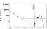
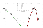
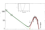
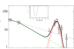
thermal dominated
Without contam.

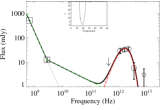
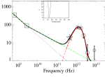
A1. continued

References

- Aird et al. (2013) Aird J. et al., 2013, ApJ, 775, 41
- Aird et al. (2010) Aird J. et al., 2010, MNRAS, 401, 2531
- Alexander et al. (2005) Alexander D. M., Bauer F. E., Chapman S. C., Smail I., Blain A. W., Brandt W. N., Ivison R. J., 2005, ApJ, 632, 736
- Amblard et al. (2010) Amblard A. et al., 2010, A&A, 518, L9
- Antonucci (1993) Antonucci R., 1993, ARA&A, 31, 473
- Antonuccio-Delogu & Silk (2010) Antonuccio-Delogu V., Silk J., 2010, MNRAS, 405, 1303
- Archibald et al. (2001) Archibald E. N., Dunlop J. S., Hughes D. H., Rawlings S., Eales S. A., Ivison R. J., 2001, MNRAS, 323, 417
- Barger et al. (2005) Barger A. J., Cowie L. L., Mushotzky R. F., Yang Y., Wang W.-H., Steffen A. T., Capak P., 2005, AJ, 129, 578
- Barvainis et al. (2005) Barvainis R., Lehár J., Birkinshaw M., Falcke H., Blundell K. M., 2005, ApJ, 618, 108
- Bavouzet et al. (2008) Bavouzet N., Dole H., Le Floc’h E., Caputi K. I., Lagache G., Kochanek C. S., 2008, A&A, 479, 83
- Becker et al. (1995) Becker R. H., White R. L., Helfand D. J., 1995, ApJ, 450, 559
- Best & Heckman (2012) Best P. N., Heckman T. M., 2012, MNRAS, 421, 1569
- Best et al. (2005) Best P. N., Kauffmann G., Heckman T. M., Ivezić Ž., 2005, MNRAS, 362, 9
- Best et al. (2014) Best P. N., Ker L. M., Simpson C., Rigby E. E., Sabater J., 2014, MNRAS, 445, 955
- Best et al. (1996) Best P. N., Longair M. S., Rottgering H. J. A., 1996, MNRAS, 280, L9
- Béthermin et al. (2010) Béthermin M., Dole H., Cousin M., Bavouzet N., 2010, A&A, 516, A43
- Bicknell et al. (2000) Bicknell G. V., Sutherland R. S., van Breugel W. J. M., Dopita M. A., Dey A., Miley G. K., 2000, ApJ, 540, 678
- Blandford & Rees (1974) Blandford R. D., Rees M. J., 1974, MNRAS, 169, 395
- Bonfield et al. (2011) Bonfield D. G. et al., 2011, MNRAS, 416, 13
- Bower et al. (2008) Bower R. G., McCarthy I. G., Benson A. J., 2008, MNRAS, 390, 1399
- Boyle & Terlevich (1998) Boyle B. J., Terlevich R. J., 1998, MNRAS, 293, L49
- Cao Orjales et al. (2012) Cao Orjales J. M. et al., 2012, MNRAS, 427, 1209
- Chapman et al. (2005) Chapman S. C., Blain A. W., Smail I., Ivison R. J., 2005, ApJ, 622, 772
- Chen et al. (2013) Chen C.-T. J. et al., 2013, ApJ, 773, 3
- Chen et al. (2015) Chen C.-T. J. et al., 2015, ApJ, 802, 50
- Cleary et al. (2007) Cleary K., Lawrence C. R., Marshall J. A., Hao L., Meier D., 2007, ApJ, 660, 117
- Condon et al. (1998) Condon J. J., Cotton W. D., Greisen E. W., Yin Q. F., Perley R. A., Taylor G. B., Broderick J. J., 1998, AJ, 115, 1693
- Condon et al. (2013) Condon J. J., Kellermann K. I., Kimball A. E., Ivezić Ž., Perley R. A., 2013, ApJ, 768, 37
- Croft et al. (2006) Croft S. et al., 2006, ApJ, 647, 1040
- Croton et al. (2006) Croton D. J. et al., 2006, MNRAS, 365, 11
- Daddi et al. (2010) Daddi E. et al., 2010, ApJ, 713, 686
- Dalton et al. (2012) Dalton G. et al., 2012, in Society of Photo-Optical Instrumentation Engineers (SPIE) Conference Series, Vol. 8446, Society of Photo-Optical Instrumentation Engineers (SPIE) Conference Series, p. 84460P
- De Breuck et al. (2005) De Breuck C., Downes D., Neri R., van Breugel W., Reuland M., Omont A., Ivison R., 2005, A&A, 430, L1
- Del Moro et al. (2013) Del Moro A. et al., 2013, A&A, 549, A59
- Dey et al. (1997) Dey A., van Breugel W., Vacca W. D., Antonucci R., 1997, ApJ, 490, 698
- Di Matteo et al. (2008) Di Matteo T., Colberg J., Springel V., Hernquist L., Sijacki D., 2008, ApJ, 676, 33
- Di Matteo et al. (2005) Di Matteo T., Springel V., Hernquist L., 2005, Nature, 433, 604
- Dicken et al. (2009) Dicken D., Tadhunter C., Axon D., Morganti R., Inskip K. J., Holt J., González Delgado R., Groves B., 2009, ApJ, 694, 268
- Dicken et al. (2012) Dicken D. et al., 2012, ApJ, 745, 172
- Dong & Wu (2016) Dong X. Y., Wu X.-B., 2016, ApJ, 824, 70
- Donoso et al. (2009) Donoso E., Best P. N., Kauffmann G., 2009, MNRAS, 392, 617
- Drouart et al. (2014) Drouart G. et al., 2014, A&A, 566, A53
- Dubois et al. (2012) Dubois Y., Devriendt J., Slyz A., Teyssier R., 2012, MNRAS, 420, 2662
- Dunlop et al. (2003) Dunlop J. S., McLure R. J., Kukula M. J., Baum S. A., O’Dea C. P., Hughes D. H., 2003, MNRAS, 340, 1095
- Dunne & Eales (2001) Dunne L., Eales S. A., 2001, MNRAS, 327, 697
- Dunne et al. (2011) Dunne L. et al., 2011, MNRAS, 417, 1510
- Dye et al. (2010) Dye S. et al., 2010, A&A, 518, L10
- Eales et al. (1997) Eales S., Rawlings S., Law-Green D., Cotter G., Lacy M., 1997, MNRAS, 291, 593
- Eales (1985) Eales S. A., 1985, MNRAS, 217, 149
- Elbaz et al. (2007) Elbaz D. et al., 2007, A&A, 468, 33
- Elbaz et al. (2011) Elbaz D. et al., 2011, A&A, 533, A119
- Emonts et al. (2011) Emonts B. H. C. et al., 2011, ApJ, 734, L25
- Evans et al. (2005) Evans A. S., Mazzarella J. M., Surace J. A., Frayer D. T., Iwasawa K., Sanders D. B., 2005, ApJS, 159, 197
- Falder et al. (2010) Falder J. T. et al., 2010, MNRAS, 405, 347
- Feigelson & Nelson (1985) Feigelson E. D., Nelson P. I., 1985, ApJ, 293, 192
- Fernandes et al. (2015) Fernandes C. A. C. et al., 2015, MNRAS, 447, 1184
- Fernandes et al. (2011) Fernandes C. A. C. et al., 2011, MNRAS, 411, 1909
- Fernandez-Conde et al. (2008) Fernandez-Conde N., Lagache G., Puget J.-L., Dole H., 2008, A&A, 481, 885
- Fernandez-Conde et al. (2010) Fernandez-Conde N., Lagache G., Puget J.-L., Dole H., 2010, A&A, 515, A48
- Floyd et al. (2004) Floyd D. J. E., Kukula M. J., Dunlop J. S., McLure R. J., Miller L., Percival W. J., Baum S. A., O’Dea C. P., 2004, MNRAS, 355, 196
- Gaibler et al. (2012) Gaibler V., Khochfar S., Krause M., Silk J., 2012, MNRAS, 425, 438
- Genzel et al. (2010) Genzel R. et al., 2010, MNRAS, 407, 2091
- Gonçalves et al. (2008) Gonçalves T. S., Steidel C. C., Pettini M., 2008, ApJ, 676, 816
- Graham & Scott (2013) Graham A. W., Scott N., 2013, ApJ, 764, 151
- Granato et al. (2001) Granato G. L., Silva L., Monaco P., Panuzzo P., Salucci P., De Zotti G., Danese L., 2001, MNRAS, 324, 757
- Griffin et al. (2010) Griffin M. J. et al., 2010, A&A, 518, L3
- Gurkan et al. (2015) Gurkan G. et al., 2015, ArXiv e-prints
- Hardcastle et al. (2013) Hardcastle M. J. et al., 2013, MNRAS, 429, 2407
- Hardcastle et al. (2007) Hardcastle M. J., Evans D. A., Croston J. H., 2007, MNRAS, 376, 1849
- Hardcastle et al. (2010) Hardcastle M. J. et al., 2010, MNRAS, 409, 122
- Häring & Rix (2004) Häring N., Rix H.-W., 2004, ApJ, 604, L89
- Harrison et al. (2012) Harrison C. M. et al., 2012, ApJ, 760, L15
- Hasinger et al. (2005) Hasinger G., Miyaji T., Schmidt M., 2005, A&A, 441, 417
- Hatch et al. (2008) Hatch N. A., Overzier R. A., Röttgering H. J. A., Kurk J. D., Miley G. K., 2008, MNRAS, 383, 931
- Hatziminaoglou et al. (2010) Hatziminaoglou E. et al., 2010, A&A, 518, L33
- Heckman & Best (2014) Heckman T. M., Best P. N., 2014, ARA&A, 52, 589
- Helou et al. (1985) Helou G., Soifer B. T., Rowan-Robinson M., 1985, ApJ, 298, L7
- Hickox et al. (2014) Hickox R. C., Mullaney J. R., Alexander D. M., Chen C.-T. J., Civano F. M., Goulding A. D., Hainline K. N., 2014, ApJ, 782, 9
- Hildebrand (1983) Hildebrand R. H., 1983, QJRAS, 24, 267
- Hill & Rawlings (2003) Hill G. J., Rawlings S., 2003, nature, 47, 373
- Ho et al. (2004) Ho P. T. P., Moran J. M., Lo K. Y., 2004, ApJ, 616, L1
- Hopkins & Elvis (2010) Hopkins P. F., Elvis M., 2010, MNRAS, 401, 7
- Hopkins & Hernquist (2006) Hopkins P. F., Hernquist L., 2006, ApJS, 166, 1
- Hopkins et al. (2005) Hopkins P. F., Hernquist L., Cox T. J., Di Matteo T., Robertson B., Springel V., 2005, ApJ, 630, 716
- Hopkins et al. (2010) Hopkins P. F., Younger J. D., Hayward C. C., Narayanan D., Hernquist L., 2010, MNRAS, 402, 1693
- Ibar et al. (2009) Ibar E., Ivison R. J., Biggs A. D., Lal D. V., Best P. N., Green D. A., 2009, MNRAS, 397, 281
- Ibar et al. (2010) Ibar E. et al., 2010, MNRAS, 409, 38
- Inskip et al. (2005) Inskip K. J., Best P. N., Longair M. S., Röttgering H. J. A., 2005, MNRAS, 359, 1393
- Inskip et al. (2008) Inskip K. J., Villar-Martín M., Tadhunter C. N., Morganti R., Holt J., Dicken D., 2008, MNRAS, 386, 1797
- Isaak et al. (2002) Isaak K. G., Priddey R. S., McMahon R. G., Omont A., Peroux C., Sharp R. G., Withington S., 2002, MNRAS, 329, 149
- Ishibashi & Fabian (2012) Ishibashi W., Fabian A. C., 2012, MNRAS, 427, 2998
- Ivezić et al. (2002) Ivezić Ž. et al., 2002, AJ, 124, 2364
- Jarvis & McLure (2002) Jarvis M. J., McLure R. J., 2002, MNRAS, 336, L38
- Jarvis & McLure (2006) Jarvis M. J., McLure R. J., 2006, MNRAS, 369, 182
- Jarvis & Rawlings (2000) Jarvis M. J., Rawlings S., 2000, MNRAS, 319, 121
- Jarvis et al. (2001a) Jarvis M. J., Rawlings S., Eales S., Blundell K. M., Bunker A. J., Croft S., McLure R. J., Willott C. J., 2001a, MNRAS, 326, 1585
- Jarvis et al. (2001b) Jarvis M. J., Rawlings S., Willott C. J., Blundell K. M., Eales S., Lacy M., 2001b, MNRAS, 327, 907
- Jarvis et al. (2010) Jarvis M. J. et al., 2010, MNRAS, 409, 92
- Jiang et al. (2007) Jiang L., Fan X., Ivezić Ž., Richards G. T., Schneider D. P., Strauss M. A., Kelly B. C., 2007, ApJ, 656, 680
- Jogee (2006) Jogee S., 2006, in Lecture Notes in Physics, Berlin Springer Verlag, Vol. 693, Physics of Active Galactic Nuclei at all Scales, Alloin D., ed., p. 143
- Johnston et al. (2015) Johnston R., Vaccari M., Jarvis M., Smith M., Giovannoli E., Häußler B., Prescott M., 2015, MNRAS, 453, 2540
- Kalfountzou et al. (2014a) Kalfountzou E., Civano F., Elvis M., Trichas M., Green P., 2014a, MNRAS, 445, 1430
- Kalfountzou et al. (2012) Kalfountzou E., Jarvis M. J., Bonfield D. G., Hardcastle M. J., 2012, MNRAS, 427, 2401
- Kalfountzou et al. (2014b) Kalfountzou E. et al., 2014b, MNRAS, 442, 1181
- Kalfountzou et al. (2011) Kalfountzou E., Trichas M., Rowan-Robinson M., Clements D., Babbedge T., Seiradakis J. H., 2011, MNRAS, 413, 249
- Karouzos et al. (2013) Karouzos M. et al., 2013, ArXiv e-prints
- Kartaltepe et al. (2012) Kartaltepe J. S. et al., 2012, ApJ, 757, 23
- Kauffmann et al. (2008) Kauffmann G., Heckman T. M., Best P. N., 2008, MNRAS, 384, 953
- Kelly et al. (2009) Kelly B. C., Vestergaard M., Fan X., 2009, ApJ, 692, 1388
- Kennicutt (1998) Kennicutt, Jr. R. C., 1998, ApJ, 498, 541
- Khochfar & Silk (2011) Khochfar S., Silk J., 2011, MNRAS, 410, L42
- Kormendy & Ho (2013) Kormendy J., Ho L. C., 2013, ARA&A, 51, 511
- Kormendy & Richstone (1995) Kormendy J., Richstone D., 1995, ARA&A, 33, 581
- Kuiper et al. (2011) Kuiper E. et al., 2011, MNRAS, 415, 2245
- Laing et al. (1983) Laing R. A., Riley J. M., Longair M. S., 1983, MNRAS, 204, 151
- Lavalley et al. (1992) Lavalley M., Isobe T., Feigelson E., 1992, in Astronomical Society of the Pacific Conference Series, Vol. 25, Astronomical Data Analysis Software and Systems I, Worrall D. M., Biemesderfer C., Barnes J., eds., p. 245
- Leipski et al. (2013) Leipski C. et al., 2013, ApJ, 772, 103
- Lutz et al. (2011) Lutz D. et al., 2011, A&A, 532, A90
- Lutz et al. (2008) Lutz D. et al., 2008, ApJ, 684, 853
- Ma & Yan (2015) Ma Z., Yan H., 2015, ApJ, 811, 58
- Madau & Dickinson (2014) Madau P., Dickinson M., 2014, ARA&A, 52, 415
- Magliocchetti et al. (2014) Magliocchetti M. et al., 2014, MNRAS, 442, 682
- Magliocchetti et al. (2016) Magliocchetti M., Lutz D., Santini P., Salvato M., Popesso P., Berta S., Pozzi F., 2016, MNRAS, 456, 431
- Magnelli et al. (2014) Magnelli B. et al., 2014, A&A, 561, A86
- Magorrian et al. (1998) Magorrian J. et al., 1998, AJ, 115, 2285
- Marconi et al. (2008) Marconi A., Axon D. J., Maiolino R., Nagao T., Pastorini G., Pietrini P., Robinson A., Torricelli G., 2008, ApJ, 678, 693
- Marconi et al. (2004) Marconi A., Risaliti G., Gilli R., Hunt L. K., Maiolino R., Salvati M., 2004, MNRAS, 351, 169
- Martínez-Sansigre & Taylor (2009) Martínez-Sansigre A., Taylor A. M., 2009, ApJ, 692, 964
- McConnell & Ma (2013) McConnell N. J., Ma C.-P., 2013, ApJ, 764, 184
- McLure & Dunlop (2004) McLure R. J., Dunlop J. S., 2004, MNRAS, 352, 1390
- McLure & Jarvis (2002) McLure R. J., Jarvis M. J., 2002, MNRAS, 337, 109
- McLure et al. (2006) McLure R. J., Jarvis M. J., Targett T. A., Dunlop J. S., Best P. N., 2006, Astronomische Nachrichten, 327, 213
- Merloni et al. (2010) Merloni A. et al., 2010, ApJ, 708, 137
- Merloni et al. (2004) Merloni A., Rudnick G., Di Matteo T., 2004, MNRAS, 354, L37
- Miyaji et al. (2015) Miyaji T. et al., 2015, ApJ, 804, 104
- Mullaney et al. (2011) Mullaney J. R., Alexander D. M., Goulding A. D., Hickox R. C., 2011, MNRAS, 414, 1082
- Mullaney et al. (2010) Mullaney J. R., Alexander D. M., Huynh M., Goulding A. D., Frayer D., 2010, MNRAS, 401, 995
- Mullaney et al. (2012a) Mullaney J. R. et al., 2012a, ApJ, 753, L30
- Mullaney et al. (2012b) Mullaney J. R. et al., 2012b, MNRAS, 419, 95
- Nesvadba et al. (2010) Nesvadba N. P. H. et al., 2010, A&A, 521, A65
- Nesvadba et al. (2011) Nesvadba N. P. H., De Breuck C., Lehnert M. D., Best P. N., Binette L., Proga D., 2011, A&A, 525, A43
- Nesvadba et al. (2006) Nesvadba N. P. H., Lehnert M. D., Eisenhauer F., Gilbert A., Tecza M., Abuter R., 2006, ApJ, 650, 693
- Netzer et al. (2007) Netzer H. et al., 2007, ApJ, 666, 806
- Nguyen et al. (2010) Nguyen H. T. et al., 2010, A&A, 518, L5
- Ott (2010) Ott S., 2010, in Astronomical Society of the Pacific Conference Series, Vol. 434, Astronomical Data Analysis Software and Systems XIX, Mizumoto Y., Morita K.-I., Ohishi M., eds., p. 139
- Padovani et al. (2011) Padovani P., Miller N., Kellermann K. I., Mainieri V., Rosati P., Tozzi P., 2011, ApJ, 740, 20
- Page et al. (2004) Page M. J., Stevens J. A., Ivison R. J., Carrera F. J., 2004, ApJ, 611, L85
- Page et al. (2001) Page M. J., Stevens J. A., Mittaz J. P. D., Carrera F. J., 2001, Science, 294, 2516
- Page et al. (2012) Page M. J. et al., 2012, Nature, 485, 213
- Papadopoulos et al. (2010) Papadopoulos P. P., van der Werf P., Isaak K., Xilouris E. M., 2010, ApJ, 715, 775
- Pascale et al. (2011) Pascale E. et al., 2011, MNRAS, 415, 911
- Penner et al. (2011) Penner K. et al., 2011, MNRAS, 410, 2749
- Pilbratt et al. (2010) Pilbratt G. L. et al., 2010, A&A, 518, L1
- Podigachoski et al. (2015) Podigachoski P. et al., 2015, A&A, 575, A80
- Poglitsch et al. (2010) Poglitsch A. et al., 2010, A&A, 518, L2
- Popesso et al. (2012) Popesso P. et al., 2012, ArXiv e-prints
- Priddey et al. (2003) Priddey R. S., Isaak K. G., McMahon R. G., Omont A., 2003, MNRAS, 339, 1183
- Ramos Almeida et al. (2012) Ramos Almeida C. et al., 2012, MNRAS, 419, 687
- Rawlings et al. (2001) Rawlings S., Eales S., Lacy M., 2001, MNRAS, 322, 523
- Rengelink et al. (1997) Rengelink R. B., Tang Y., de Bruyn A. G., Miley G. K., Bremer M. N., Roettgering H. J. A., Bremer M. A. R., 1997, A&AS, 124, 259
- Richards et al. (2006) Richards G. T. et al., 2006, AJ, 131, 2766
- Rigby et al. (2015) Rigby E. E., Argyle J., Best P. N., Rosario D., Röttgering H. J. A., 2015, A&A, 581, A96
- Rigby et al. (2011) Rigby E. E., Best P. N., Brookes M. H., Peacock J. A., Dunlop J. S., Röttgering H. J. A., Wall J. V., Ker L., 2011, MNRAS, 416, 1900
- Rodighiero et al. (2015) Rodighiero G. et al., 2015, ApJ, 800, L10
- Rosario et al. (2012) Rosario D. J. et al., 2012, A&A, 545, A45
- Rosario et al. (2013) Rosario D. J. et al., 2013, A&A, 560, A72
- Rovilos et al. (2012) Rovilos E. et al., 2012, A&A, 546, A58
- Rowan-Robinson (1995) Rowan-Robinson M., 1995, MNRAS, 272, 737
- Salviander et al. (2007) Salviander S., Shields G. A., Gebhardt K., Bonning E. W., 2007, ApJ, 662, 131
- Sánchez et al. (2004) Sánchez S. F. et al., 2004, ApJ, 614, 586
- Santini et al. (2010) Santini P. et al., 2010, A&A, 518, L154
- Santini et al. (2012) Santini P. et al., 2012, A&A, 540, A109
- Sargent et al. (2013) Sargent B. A., Patel N. A., Meixner M., Otsuka M., Riebel D., Srinivasan S., 2013, ApJ, 765, 20
- Sargent et al. (2010) Sargent M. T. et al., 2010, ApJS, 186, 341
- Schneider et al. (2005) Schneider D. P. et al., 2005, AJ, 130, 367
- Schreiber et al. (2015) Schreiber C. et al., 2015, A&A, 575, A74
- Schulze & Wisotzki (2010) Schulze A., Wisotzki L., 2010, A&A, 516, A87
- Schweitzer et al. (2006) Schweitzer M. et al., 2006, ApJ, 649, 79
- Seymour et al. (2007) Seymour N. et al., 2007, ApJS, 171, 353
- Seymour et al. (2011) Seymour N. et al., 2011, MNRAS, 413, 1777
- Shabala & Godfrey (2013) Shabala S. S., Godfrey L. E. H., 2013, ApJ, 769, 129
- Shankar (2010) Shankar F., 2010, in IAU Symposium, Vol. 267, IAU Symposium, pp. 248–253
- Shankar et al. (2004) Shankar F., Salucci P., Granato G. L., De Zotti G., Danese L., 2004, MNRAS, 354, 1020
- Shao et al. (2010) Shao L. et al., 2010, A&A, 518, L26
- Shen et al. (2008) Shen Y., Greene J. E., Strauss M. A., Richards G. T., Schneider D. P., 2008, ApJ, 680, 169
- Shen et al. (2011) Shen Y. et al., 2011, ApJS, 194, 45
- Shi et al. (2005) Shi Y. et al., 2005, ApJ, 629, 88
- Silk et al. (2012) Silk J., Antonuccio-Delogu V., Dubois Y., Gaibler V., Haas M. R., Khochfar S., Krause M., 2012, A&A, 545, L11
- Silk & Nusser (2010) Silk J., Nusser A., 2010, ApJ, 725, 556
- Smith (2015) Smith D. J. B., 2015, ArXiv e-prints
- Smith et al. (2013) Smith D. J. B. et al., 2013, MNRAS, 436, 2435
- Somerville et al. (2008) Somerville R. S., Hopkins P. F., Cox T. J., Robertson B. E., Hernquist L., 2008, MNRAS, 391, 481
- Spinrad et al. (1985) Spinrad H., Marr J., Aguilar L., Djorgovski S., 1985, PASP, 97, 932
- Springel et al. (2005) Springel V. et al., 2005, Nature, 435, 629
- Stanley et al. (2015) Stanley F., Harrison C. M., Alexander D. M., Swinbank A. M., Aird J. A., Del Moro A., Hickox R. C., Mullaney J. R., 2015, MNRAS, 453, 591
- Steinhardt & Elvis (2010) Steinhardt C. L., Elvis M., 2010, MNRAS, 402, 2637
- Stevens et al. (2003) Stevens J. A. et al., 2003, Nature, 425, 264
- Treister et al. (2012) Treister E., Schawinski K., Urry C. M., Simmons B. D., 2012, ApJ, 758, L39
- Trichas et al. (2012) Trichas M. et al., 2012, ApJS, 200, 17
- Trichas et al. (2010) Trichas M. et al., 2010, MNRAS, 405, 2243
- Urrutia et al. (2008) Urrutia T., Lacy M., Becker R. H., 2008, ApJ, 674, 80
- van Breugel et al. (2004) van Breugel W., Fragile C., Anninos P., Murray S., 2004, in IAU Symposium, Vol. 217, Recycling Intergalactic and Interstellar Matter, Duc P.-A., Braine J., Brinks E., eds., p. 472
- van Haarlem et al. (2013) van Haarlem M. P. et al., 2013, A&A, 556, A2
- Vardoulaki et al. (2010) Vardoulaki E. et al., 2010, MNRAS, 401, 1709
- Venemans et al. (2007) Venemans B. P. et al., 2007, A&A, 461, 823
- Virdee et al. (2013) Virdee J. S. et al., 2013, MNRAS, 432, 609
- Wagner et al. (2012) Wagner A. Y., Bicknell G. V., Umemura M., 2012, ApJ, 757, 136
- Wall et al. (2005) Wall J. V., Jackson C. A., Shaver P. A., Hook I. M., Kellermann K. I., 2005, A&A, 434, 133
- Wang et al. (2009) Wang J.-G. et al., 2009, ApJ, 707, 1334
- Wardlow et al. (2011) Wardlow J. L. et al., 2011, MNRAS, 415, 1479
- White et al. (2007) White R. L., Helfand D. J., Becker R. H., Glikman E., de Vries W., 2007, ApJ, 654, 99
- Whittam et al. (2013) Whittam I. H. et al., 2013, MNRAS, 429, 2080
- Whittam et al. (2015) Whittam I. H., Riley J. M., Green D. A., Jarvis M. J., Vaccari M., 2015, MNRAS, 453, 4244
- Willott et al. (1998) Willott C. J., Rawlings S., Blundell K. M., Lacy M., 1998, MNRAS, 300, 625
- Willott et al. (1999) Willott C. J., Rawlings S., Blundell K. M., Lacy M., 1999, MNRAS, 309, 1017
- Willott et al. (2001) Willott C. J., Rawlings S., Blundell K. M., Lacy M., Eales S. A., 2001, MNRAS, 322, 536
- Xue et al. (2010) Xue Y. Q. et al., 2010, ApJ, 720, 368
- Younger et al. (2008) Younger J. D. et al., 2008, ApJ, 688, 59