An exactly solvable quench protocol for integrable spin models

Abstract

Quantum quenches in continuum field theory across critical points are known to display different scaling behaviours in different regimes of the quench rate. We extend these results to integrable lattice models such as the transverse field Ising model on a one-dimensional chain and the Kitaev model on a two-dimensional honeycomb lattice using a nonlinear quench protocol which allows for exact analytical solutions of the dynamics. Our quench protocol starts with a finite mass gap at early times and crosses a critical point or a critical region, and we study the behaviour of one point functions of the quenched operator at the critical point or in the critical region as a function of the quench rate. For quench rates slow compared to the initial mass gap, we find the expected Kibble-Zurek scaling. In contrast, for rates fast compared to the mass gap, but slow compared to the inverse lattice spacing, we find scaling behaviour similar to smooth fast continuum quenches. For quench rates of the same order of the lattice scale, the one point function saturates as a function of the rate, approaching the results of an abrupt quench. The presence of an extended critical surface in the Kitaev model leads to a variety of scaling exponents depending on the starting point and on the time where the operator is measured. We discuss the role of the amplitude of the quench in determining the extent of the slow (Kibble-Zurek) and fast quench regimes, and the onset of the saturation.

1 Introduction

The dynamics of a closed quantum system following a smooth quench involving a critical point is expected to carry universal signatures of the critical theory. Of course, the best known of such behaviours would be Kibble-Zurek (KZ) scaling kibble ; zurek , which has received considerable attention in the past several years more ; qcritkz . One might characterize the corresponding quenches as “slow” since they involve a protocol where the evolution remains adiabatic until the system approaches very close to the critical point. However, recent holographic studies numer ; fastQ also revealed interesting new scaling behaviour when critical points were probed by “fast” quench protocols. Later examination showed that this fast quench scaling is a universal behaviour for quantum field theories flowing from a UV fixed point, which is described by the conformal field theory dgm1 ; dgm2 ; dgm3 . Hence various renormalized observables in such continuum systems can exhibit a variety of scaling behaviours for different regimes of the quench rate. In fact, it was explicitly shown in dgm4 that scaling behaviour of various (renormalized) observables smoothly interpolates between the Kibble-Zurek scaling and the fast quench scaling with appropriate quench protocols in free scalar and fermion field theories.

However, the above results beg the question: how do these scaling regimes manifest in the presence of a finite UV cutoff? This question is particularly important if we wish to make any contact with real experimental systems which always have a finite lattice spacing (e.g., cold atom systems in optical lattices). The observables of interest are now bare quantities, and while we can vary the quench rate over a broad range of scales, the cutoff scale (e.g., the inverse lattice spacing) will always place limitations on fast quench protocols. However, we might still expect that when the quench rate is taken far below the cutoff scale, the results would match those for renormalized quantities for the corresponding continuum fixed point theory.

In this paper, we will explore quench dynamics in spin systems with a smooth nonlinear quench protocol for which the quantum dynamics can be solved exactly for any value of the quench rate. We will focus on two such models: the transverse field Ising model in one space dimension and the Kitaev honeycomb model kitaev in two space dimensions. The ability to solve the dynamics stems from the fact that both these models can be written in terms of free fermions in momentum space. In both cases, we will measure the expectation value of the quenched operator, which in the fermionic language is ${\bar{\psi}}\psi$, where $\psi$ is the fermionic field used to represent the integrable spin models via Jordan-Wigner transformation.

For quenches where the couplings vary linearly in time, the response of the (1+1)-dimensional Ising model has been examined in dziarmaga , while the Kitaev model has been studied in sengupta ; hikichi . Both the Ising powell ; cc2 and the Kitaev kquench1 ; kquench2 model have also been studied for instantaneous quenches. In contrast, we will study the quench protocols in which the couplings vary smoothly over a (finite) time interval (characterized by the duration $\delta t$) and saturate to constant values at early and late times. Among other things, this allows us to investigate the dependence on the quench rate and the amplitude of the quench separately, and to scan the entire range of quench rates, including the new fast scaling regime dgm1 ; dgm2 ; dgm3 ; dgm4 , as well as the regime where the quench rate becomes of the order of the UV cutoff. In the latter regime the response saturates as a function of the quench rate, as one expects for an instantaneous quench. However we find that the $\delta t$ at which this saturation happens is proportional to the amplitude for large amplitudes, while it is independent of the amplitude for small amplitudes.

While the Ising model has an isolated critical point separating two gapped phases, the Kitaev model is particularly interesting since there is a whole critical region in the space of couplings. This allows us to study a new class of quenches in which the couplings are varied entirely within this critical region.

The remainder of the paper is organized as follows: The remainder of this section provides a more detailed review of the various quench regimes, which we introduced in the introductory discussion above. In section 2, we review the two lattice models and in particular, we derive the relevant continuum theory describing the corresponding critical points. We then introduce our specific quench profiles for the couplings and discuss the exact time-dependent solutions in section 3. Our various results for the response of these lattice models in different quench regimes are presented in section 4. Section 5 contains a brief discussion of our results. In appendix A, we derive the fast scaling behaviour using linear response theory around a CFT in arbitrary dimensions. In appendix B, we provide some technical details required to understand the amplitude dependence of the value of $\delta t$ at which the response saturates. The final appendix C discusses the Cluster Ising model on a one-dimensional closed chain, which can also be studied in the same manner as the Ising model.

1.1 Quench regimes: Slow, Fast and Instantaneous

Slow Quench: For a quench protocol where the system starts with a finite mass gap and then crosses or approaches a critical point, at a rate which is slow compared to the initial gap, many systems show Kibble-Zurek (KZ) scaling kibble ; zurek ; more ; qcritkz . Consider examining a relativistic system (i.e., the dynamical critical exponent is $z=1$) with the simple power-law protocol

$$g(t)-g_{c}\sim g_{0}\ \left({t}/{\delta t}\right)^{r}\,.$$ (1)

It follows that the instantaneous energy gap $E_{g}(t)$ is given by

$$E_{g}(t)=\kappa\,|g(t)-g_{c}|^{\nu}=E_{0}\ |t/\delta t|^{r\nu}\,,$$ (2)

where $\nu$ is the correlation length exponent for the critical point. Now the initial adiabatic evolution breaks down at $t=-t_{KZ}$, as determined by the Landau criterion

$$\frac{1}{E_{g}(t)^{2}}\frac{dE_{g}(t)}{dt}\bigg{|}_{t=-t_{KZ}}\sim 1\,.$$ (3)

Then the early-time one-point function of an operator ${\cal O}_{\Delta}$ with conformal dimension $\Delta$ is expected to exhibit Kibble-Zurek scaling:

$$\langle{\cal O}_{\Delta}(t)\rangle\sim(t_{KZ})^{-\Delta}~{}F(t/t_{KZ})\,.$$ (4)

There are similar KZ scaling relationships for correlation functions. Given the profile (2) above, one finds that $t_{KZ}$ is related to the inverse quench rate $\delta t$ by the scaling relation

$$t_{KZ}\sim\left(\frac{\delta t^{r\nu}}{E_{0}}\right)^{\frac{1}{r\nu+1}}\,.$$ (5)

We will be considering more general quench protocols where the instantaneous energy gap takes the form

$$E_{g}(t)=E_{0}\,f(t/\delta t)\,,$$ (6)

where the function $f(x)\rightarrow 1$ at $x\rightarrow-\infty$. Only in the regime $x\ll 1$ does the profile $f(x)$ approach zero as $f(x)\sim x^{r\nu}$. Now imagine that the system starts in its ground state at $t=-\infty$ and initially evolves adiabatically since $E_{g}(t)$ is only changing very slowly. However, as described above, this initial adiabatic evolution breaks down when the Landau criterion (3) is satisfied. At this point, the Kibble-Zurek scaling (4) described above can appear if two conditions are satisfied: (i) $t_{KZ}$ is such that the function $f(x)$ can be approximated by the power law $x^{r\nu}$, i.e., we must demand that $t_{KZ}\ll\delta t$; and (ii) at $t=-t_{KZ}$, the instantaneous gap is much smaller than the UV cutoff scale $\Lambda_{\textrm{\tiny UV}}$, i.e., we require $E_{KZ}\equiv E_{g}(t=-t_{KZ})\ll\Lambda_{\textrm{\tiny UV}}$. Combining Eq. (5) with the first condition yields

$$\delta t\gg 1/E_{0}\,.$$ (7)

Similarly, the second condition can be expressed as

$$\delta t\gg\frac{1}{E_{0}}\left(\frac{E_{0}}{\Lambda_{\textrm{\tiny UV}}}\right)^{1+\frac{1}{r\nu}}\,.$$ (8)

When $E_{0}\ll\Lambda_{\textrm{\tiny UV}}$, the condition (7) implies the condition (8). However, when $E_{0}$ is of the same order or larger than $\Lambda_{\textrm{\tiny UV}}$, the condition (8) is the stronger restriction. Note that we are considering protocols where $E_{0}>E_{KZ}$ .

This approach is closely related to quench protocols used more commonly in discussions of KZ behaviour in the condensed matter literature, where the behaviour (2) is often considered to hold for all times. In particular, if we define $K\equiv E_{0}/\delta t^{r\nu}$, the expression (2) for the instantaneous gap becomes $E_{g}(t)=K\,t^{r\nu}$. Note that in this case $E_{0}$ and $\delta t$ can not be separately varied. The system is prepared in the ground state of the theory at some (finite) initial time $t=t_{i}$. The KZ time and energy gap are then given by $t_{KZ}=K^{-\frac{1}{r\nu+1}}$ and $E_{KZ}=K^{\frac{1}{r\nu+1}}$, respectively. Now the first condition above is replaced by $|t_{i}|\geq t_{KZ}$, which can be equivalently written as

$$K<E(t_{i})^{r\nu+1}\,.$$ (9)

The second condition above, i.e., $E_{KZ}\ll\Lambda_{\textrm{\tiny UV}}$, can be expressed as

$$K\ll\Lambda_{\textrm{\tiny UV}}^{r\nu+1}\,.$$ (10)

Hence if $E(t_{i})<\Lambda_{\textrm{\tiny UV}}$, the first condition implies the first, while if $E(t_{i})\gtrsim\Lambda_{\textrm{\tiny UV}}$, the second constraint is the stronger one. Often one actually considers the situation where $t_{i}\to-\infty$. In this case, the only constraint is Eq. (10), since $E(t_{i})$ diverges rendering the inequality (9) trivial.

Fast Quench: As noted above, recently a new scaling behaviour was discovered for smooth but fast quenches. In particular, consider a generic action

$$S=S_{\textrm{\tiny CFT}}+\int dt\int d^{d-1}x~{}\lambda(t)\,{\cal O}_{\Delta}(x,t)\,,$$ (11)

where $S_{\textrm{\tiny CFT}}$ is the conformal field theory action describing the UV fixed point, and ${\cal O}_{\Delta}$ is a relevant operator with conformal dimension $\Delta$. The quench profile for coupling $\lambda(t)$ starts from some initial value $\lambda_{\textrm{\tiny init}}$ and smoothly changes to the final value $\lambda_{\textrm{\tiny fin}}$ over a time scale $\delta t$. If this time scale is fast compared to all physical scales, but slow compared to the scale of the UV cutoff, i.e.,

$$\Lambda_{\textrm{\tiny UV}}^{-1}\ll\delta t\ll\lambda_{\textrm{\tiny init}}^{1/(\Delta-d)}\,,\lambda_{\textrm{\tiny fin}}^{1/(\Delta-d)}\,,|\lambda_{\textrm{\tiny fin}}-\lambda_{\textrm{\tiny init}}|^{1/(\Delta-d)}\,,$$ (12)

then the response of various renormalized quantities exhibit scaling at early times dgm1 ; dgm2 ; dgm3 ; dgm4 . For example, during the quench process, the renormalized expectation value $\langle{\cal O}_{\Delta}\rangle_{ren}$ behaves as

$$\langle{\cal O}_{\Delta}\rangle_{ren}\sim\frac{\delta\lambda}{\delta t^{2\Delta-d}}\,.$$ (13)

where $\delta\lambda=\lambda_{\textrm{\tiny fin}}-\lambda_{\textrm{\tiny init}}$. Similarly, the energy density scales as

$${\cal{E}}_{ren}\sim\frac{\delta\lambda^{\,2}}{\delta t^{2\Delta-d}}\,.$$ (14)

This scaling behaviour was originally discovered in holographic computations numer ; fastQ but then it was shown to hold in free field theories, and further argued to be true for general interacting theories dgm1 ; dgm2 .

It may seem mysterious that the underlying QFT has been regulated and renormalized and yet the above expressions are divergent in the limit $\delta t\to 0$, when $\Delta>d/2$. These divergences arise because as $\delta t$ shrinks, the quench is exciting a growing number of short wavelength modes. Further there is an infinite “reservoir” of such modes available as long as they are arranged as excitations of the UV fixed-point CFT. Implicitly the latter holds for renormalized quantities as in Eqs. (13) and (14), which are defined in a procedure which involves taking the limit $\Lambda_{\textrm{\tiny UV}}\to\infty$. Of course, if the cutoff scale $\Lambda_{\textrm{\tiny UV}}$ is held fixed while $\delta t$ continues to shrink, eventually we will encounter $\delta t\sim 1/\Lambda_{\textrm{\tiny UV}}$ and the above scaling behaviour will no longer be applicable.

Instantaneous Quench: The approach, which is most commonly discussed in the quantum quench literature, e.g., powell ; cc2 ; cc3 ; more , involves preparing a system in the ground state of an initial Hamiltonian and then time evolving this state with a new or final Hamiltonian. There are some scaling results known to hold in the situation where the ground state of the initial Hamiltonian is gapped and the final Hamiltonian corresponds to a critical phase cc2 ; cc3 , in particular, the latter is a (1+1)-dimensional CFT. One can imagine that this describes an instantaneous quench, where initially the couplings of Hamiltonian are held constant, then at a single moment of time, the couplings are instantaneously changed to produce the final Hamiltonian and subsequently the couplings are fixed at their new values. Further this interpretation naively suggests that this protocol corresponds to the $\delta t\to 0$ limit of the smooth fast quenches described above. However, as emphasized in dgm2 ; dgm3 , this limit does not reproduce the instantaneous quench because implicitly the former assumes that quench rate is always small compared to the UV cutoff, i.e., $\Lambda_{\textrm{\tiny UV}}\gg 1/\delta t$. Instead, the instantaneous quench implicitly assumes that $\delta t\to 0$ while $\Lambda_{\textrm{\tiny UV}}$ remains fixed.

While the above discussion applies quite generally, implicitly we are assuming $2\Delta>d$ in which case Eqs. (13) and (14) would produce divergences in the limit $\delta t\to 0$. However, we can also consider the situation where $2\Delta<d$ in which case the expressions in these formulae would vanish when $\delta t\to 0$. In fact, these expressions no longer capture the leading contributions in this situation and instead the quench will produce finite results for $\langle{\cal O}_{\Delta}\rangle_{ren}$ and ${\cal{E}}_{ren}$. In this case, the results in free field theories indicate that these final answers do not depend on UV details and the responses for the instantaneous and the smooth quenches will agree dgm3 . This behaviour is also manifest in the excess energy above the adiabatic value at late times, which is UV finite for any finite $\delta t$. Here again free field studies dgm3 show that for $2\Delta<d$, this quantity remains finite in the $\delta t\rightarrow 0$ limit and reproduces instantaneous quench results. Instead it is a subleading term which displays scaling behaviour analogous to that in Eq. (14). For $2\Delta>d$ the smooth quench answers diverge in this $\delta t\rightarrow 0$ limit displaying scaling, while the instantaneous quench answer has a UV divergence.

Having introduced a finite UV cutoff in the present paper, we are certainly able to study the new regime where $\Lambda_{\textrm{\tiny UV}}\lesssim 1/\delta t$, which we will refer to as the instantaneous quench regime. As noted above, the fast quench scaling does not apply in this regime. In particular, the divergences which the $\delta t\to 0$ limit would produce in Eq. (13) are avoided and instead we will see that the response saturates when we enter the instantaneous quench regime.

An interesting feature of this regime is that for protocols of the form (6), the value of $\delta t$ where this saturation occurs is independent of the amplitude $E_{0}$ for small amplitudes, while it becomes proportional to $E_{0}$ for $E_{0}\sim O(\Lambda_{\textrm{\tiny UV}})$ or larger. We provide a physical explanation of this behaviour in terms of the value of $\delta t$ at which the largest momentum mode $k_{max}$ (in lattice units) contributing to the observable departs from adiabatic behaviour. A detailed study of the Ising model reveals that for large amplitudes $k_{max}$ is at the UV cutoff, i.e., $k_{max}\sim\pi$. The Landau criterion for this mode leads to the above result. In other words, saturation happens when all possible modes get excited. On the other hand, we find that for small amplitudes $k_{max}\propto E_{0}$, i.e., all modes do not contribute significantly to the observable we calculate. In this case, the Landau criterion shows that the saturation value is independent of the amplitude.

2 The models

In this section, we will describe the lattice models of interest and set our notation.

2.1 Transverse Field Ising Model

We write the Hamiltonian for the transverse field Ising model as

$$H_{\textrm{\tiny Ising}}=-\sum_{n}\left[h(t)\,\tau^{(3)}(n)+J\,\tau^{(1)}(n)\,\tau^{(1)}(n+1)\right]\,,$$ (15)

where $\tau^{(i)}$ denote the Pauli spin operators, and $n$ denotes the site indices of the one-dimensional chain. The time dependent coupling $h(t)$ denotes the transverse magnetic field and $J$ is the interaction strength between the nearest-neighbor spins. Both couplings have dimensions of energy here. We will follow the conventions of kogut . Using the well-known Jordan-Wigner transformation, the Hamiltonian given by Eq. (15) can be rewritten as the theory of a one-component fermion $c(n)$ at each site, whose Fourier components will be denoted by $d(q)$,

$$c(n)=\frac{e^{-\frac{i\pi}{4}}}{\sqrt{2N+1}}\sum_{m=-N}^{N}e^{-iqn}d(q)\qquad{\rm with}\ \ \ q=\frac{2\pi m}{2N+1}\,.$$ (16)

The latter have the usual anti-commutation relations

$$\{d(q),d^{\dagger}(q^{\prime})\}=\delta_{mm^{\prime}}\ ,\qquad\{d(q),d(q^{\prime})\}=\{d^{\dagger}(q),d^{\dagger}(q^{\prime})\}=0\,.$$ (17)

Note that $q$ is periodic from Eq. (16), i.e., the expression is invariant under $q\to q+2\pi$. However, it is convenient to shift the momenta

$$q\rightarrow k=q-\pi\,,$$ (18)

and to introduce a two-component Majorana fermion

$$\chi(k)=\left(\begin{array}[]{c}d(k+\pi)\\ d^{\dagger}(-k-\pi)\end{array}\right)\,.$$ (19)

The Hamiltonian then becomes

$$H_{\textrm{\tiny Ising}}=2J\sum_{k>0}\chi^{\dagger}(k)\left[(\cos k-g(t))\,\sigma_{3}+\sin k\,\sigma_{1}\right]\chi(k)\,,$$ (20)

where $\sigma_{i}$ denote Pauli matrices in the particle-hole space of fermions and we have introduced the (dimensionless) coupling $g(t)=h(t)/J$. Note that the momentum sum runs over half the Brillouin zone kogut . Now it is convenient to consider the limit $N\to\infty$, in which we are considering an infinite chain of spins. This will certainly remove the possibility of having our quench results infected by any finite size effects. In this limit, the momentum $k$ becomes a continuous variable on the range $[-\pi,\pi]$ — although as noted above, $k\sim k+2\pi$. We would have the more or less standard replacements:

$$\frac{1}{2N+1}\sum_{m=-N}^{N}\ \longrightarrow\ \frac{1}{2\pi}\int_{-\pi}^{\pi}dk\quad{\rm and}\quad(2N+1)\,\delta_{mm^{\prime}}\ \longrightarrow\ 2\pi\,\delta(k-k^{\prime})\,.$$ (21)

Hence it is convenient to rescale operators $\hat{d}(k)=\sqrt{2N+1}\,d(k)$ so that in the continuous limit, the anti-commutation (17) become

$$\{\hat{d}(k),\hat{d}^{\dagger}(k^{\prime})\}=2\pi\,\delta(k-k^{\prime})\qquad,\qquad\{{\hat{d}}(k),{\hat{d}}(k^{\prime})\}=\{{\hat{d}}^{\dagger}(k),{\hat{d}}^{\dagger}(k^{\prime})\}=0\,.$$ (22)

Now constructing the fermion ${\hat{\chi}}(q)$ from these rescaled operators as in Eq. (19), the Hamiltonian (20) becomes

$$H_{\textrm{\tiny Ising}}=2J\int_{0}^{\pi}\frac{dk}{2\pi}\ {\hat{\chi}}^{\dagger}(k)\left[(\cos k-g(t))\,\sigma_{3}+\sin k\,\sigma_{1}\right]{\hat{\chi}}(k)\,.$$ (23)

For a given momentum $k$, the instantaneous energy eigenvalues are given by

$$E=\pm 2J\sqrt{(\cos k-g(t))^{2}+\sin^{2}k}\,.$$ (24)

This dispersion relation makes clear that $g=1$ corresponds to a critical point where the gapless mode is $k=0$.

The critical point at $g=1$ separates two massive phases (the paramagnetic and the ferromagnetic phases of the Ising model), and the continuum limit around this critical point is a massive Majorana fermion. This may be seen as usual by first expanding around the critical coupling with

$$g=1-\epsilon(t)\,,$$ (25)

and then explicitly introducing the lattice spacing $a$ to define the following dimensionful quantities:

$$p=k/a\,,\qquad m(t)=\epsilon(t)/a\,,\quad{\rm and}\quad\psi(p)=a^{1/2}\,{\hat{\chi}}(a\,p)\,.$$ (26)

Finally we also define the dimensionless spin coupling: ${\hat{J}}=J\,a$. We then take the continuum limit with $a\rightarrow 0$ holding ${\hat{J}}$, $p$, $m(t)$, and $\psi(p)$ fixed. In this limit, all of the terms in $H_{\textrm{\tiny Ising}}$ which are higher order in $a$ vanish and we are left with the continuum Hamiltonian,

$$H_{\textrm{\tiny Ising}}^{\textrm{\tiny cont}}=2{\hat{J}}\int_{0}^{\infty}\frac{dp}{2\pi}\ \psi^{\dagger}(p)\left[m(t)\,\sigma_{3}+p\,\sigma_{1}\right]\psi(p)\,,$$ (27)

which corresponds to the theory of a massive Majorana fermion with a (time dependent) mass $m(t)$.

Before ending this subsection, we note that another related integrable model which shows similar behaviour is the Cluster-Ising model on a one-dimensional closed chain. This model is reviewed in appendix C, where it is shown that the corresponding Hamiltonian can be reduced to three copies of the continuum Ising Hamiltonian (27). Thus the exactly solvable quench protocols, which we will discuss below, also apply to the Cluster-Ising model.

2.2 Kitaev Honeycomb Model

This model in $2+1$ dimensions is defined on a (spatial) honeycomb lattice. The Hamiltonian can be written as

$$H_{\textrm{\tiny Kitaev}}=\sum_{j+l={\rm even}}\left[J_{1}\,\tau^{(1)}_{j,l}\tau^{(1)}_{j+1,l}+J_{2}\,\tau^{(2)}_{j,l}\tau^{(2)}_{j-1,l}+J_{3}\,\tau^{(3)}_{j,l}\tau^{(3)}_{j,l+1}\right]\,.$$ (28)

where $(j,l)$ denote the column and row indices of a site on the lattice. Typically, $(2+1)$-dimensional models are not solvable, however, remarkably this model can be solved exactly for constant couplings $J_{i}$ kitaev , by rewriting it as a fermionic theory. We will use the fermionic theory, which results from the Jordan-Wigner transformation given in nussinov ; feng . The latter introduces two sets of real fermionic fields obeying the standard anti-commutation relations. To express the Hamiltonian in terms of these fermionic fields, we first denote the unit vectors in the $x$ and $y$ directions by $\hat{\bf i}$ and $\hat{\bf j}$, respectively — see figure 1. Then the vectors

$$\vec{M}_{1}=\frac{\sqrt{3}}{2}\,\hat{\bf i}+\frac{3}{2}\,\hat{\bf j}\,,\qquad\vec{M}_{2}=\frac{\sqrt{3}}{2}\,\hat{\bf i}-\frac{3}{2}\,\hat{\bf j}\,,$$ (29)

span the reciprocal lattice. We also define the vectors,

$${\vec{n}}=\sqrt{3}\,n_{1}\,\hat{\bf i}+n_{2}\left(\frac{\sqrt{3}}{2}\,\hat{\bf i}+\frac{3}{2}\,\hat{\bf j}\right)\,,$$ (30)

where $n_{1}$ and $n_{2}$ are integers. The vectors ${\vec{n}}$ denote the midpoints of the vertical bonds in the honeycomb lattice, i.e., the lattice sites are positioned at ${\vec{n}}\pm\hat{\bf j}/2$.

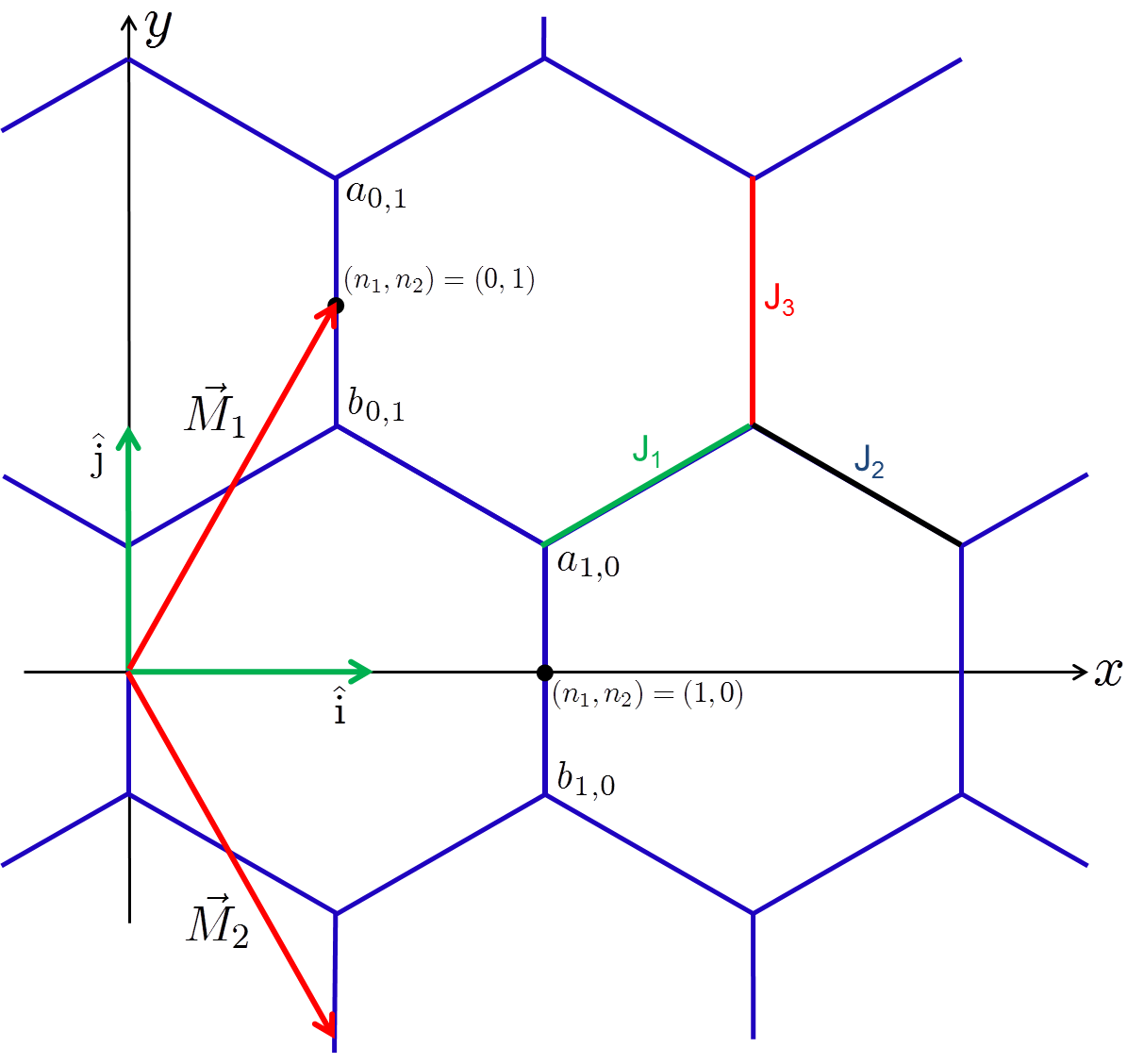
Figure 1: The honeycomb lattice on which the Kitaev model (31) is defined. $J_{1}$ and $J_{2}$ correspond to the interaction strength on the horizontal bonds tilted upward and downward, respectively, while $J_{3}$ defines the interaction strength for the vertical bonds. The fermions $a_{{\vec{n}}}$ and $b_{{\vec{n}}}$ live on the sites at the top and bottom of the vertical bond labeled by ${{\vec{n}}}$.

The Hamiltonian (28) can now be written as

$$H_{\textrm{\tiny Kitaev}}=i\sum_{{\vec{n}}}[J_{1}\,b_{{\vec{n}}}a_{{\vec{n}}-\vec{M}_{1}}+J_{2}\,b_{{\vec{n}}}a_{{\vec{n}}+\vec{M}_{2}}+J_{3}\,D_{{\vec{n}}}\,b_{{\vec{n}}}a_{{\vec{n}}}]\,,$$ (31)

where the fermion $a_{{\vec{n}}}$ lives on the site at the top of the vertical bond labeled by ${{\vec{n}}}$ while the fermion $b_{{\vec{n}}}$ lives on the bottom site — see figure 1. The quantity $D_{{\vec{n}}}$ is an operator which is bilinear in the fermions, can take values $\pm 1$ on each link, and commutes with the Hamiltonian. This allows us to think of $D_{{\vec{n}}}$ as representing a static $Z_{2}$ gauge field living on the links of the honeycomb lattice, which is coupled to the fermions. The key point which makes the Kitaev model integrable is that $D_{\vec{n}}$ is conserved leading to an infinite number of conserved quantities; the ground state sector of the model corresponds to choice of $D_{\vec{n}}=1$ on each link kitaev .

In the following, we will study quantum quench from the ground state in this model with protocols where $J_{1}$ and $J_{2}$ are held constant but $J_{3}$ is time dependent. Since the $D_{{\vec{n}}}$ commute with $H_{\rm Kitaev}$, they remain unity throughout the full dynamics. In this case, we can set $D_{{\vec{n}}}=1$ in Eq. (31) making the time dependent Hamiltonian quadratic in the fermions.

Now let us first define the Fourier modes $a_{\vec{k}}$ and $b_{\vec{k}}$

$$\left(\begin{array}[]{c}a_{\vec{n}}\\ b_{\vec{n}}\end{array}\right)=\sqrt{\frac{4}{N}}\sum_{\vec{k}}\left[\left(\begin{array}[]{c}a_{\vec{k}}\\ b_{\vec{k}}\end{array}\right)e^{i{\vec{k}}\cdot{\vec{n}}}+\left(\begin{array}[]{c}a^{\dagger}_{\vec{k}}\\ b^{\dagger}_{\vec{k}}\end{array}\right)e^{-i{\vec{k}}\cdot{\vec{n}}}\right]\,,$$ (32)

where $N$ is the total number of sites (assumed to be even) and ${\vec{k}}$ extends over half the Brillouin zone. We then define a two-component spinor sengupta

$$\chi_{\vec{k}}=\frac{1}{\sqrt{2}}\left(\begin{array}[]{c}a_{\vec{k}}+ib_{\vec{k}}\\ i(a_{\vec{k}}-ib_{\vec{k}})\end{array}\right)\,.$$ (33)

The Hamiltonian (31) with a time dependent $J_{3}$ then becomes

$$H_{\textrm{\tiny Kitaev}} = 2\int\frac{d^{2}k}{4\pi^{2}}\,\chi^{\dagger}({\vec{k}})\Big{[}(J_{3}(t)+J_{1}\cos k_{1}+J_{2}\cos k_{2})\,\sigma_{3}$$ (34)

$$\qquad\qquad\qquad\qquad+(J_{1}\sin k_{1}-J_{2}\sin k_{2})\,\sigma_{1}\Big{]}\chi({\vec{k}})\,,$$

where $\sigma_{i}$ denote Pauli matrices in the space of fermions and we have defined

$$k_{1}\equiv{\vec{k}}\cdot\vec{M}_{1}\,,\qquad k_{2}\equiv{\vec{k}}\cdot\vec{M}_{2}\,.$$ (35)

Implicitly, we are again considering the limit of an infinite lattice size, which has resulted in replacing the momentum sum with an integral in Eq. (35). The measure is defined as $d^{2}k\equiv dk_{1}dk_{2}$, where the range of the integral is $0\leq k_{1},k_{2}\leq\pi$ sengupta .

For constant $J_{3}$, the model is critical over a two-dimensional region in the $(J_{1},J_{2},J_{3})$ hyperplane. Indeed the gap vanishes when

$$\cos k_{1}=-\frac{J_{3}^{2}+J_{1}^{2}-J_{2}^{2}}{2J_{3}J_{1}}\,,\qquad \quad\cos k_{2}=-\frac{J_{3}^{2}+J_{2}^{2}-J_{1}^{2}}{2J_{3}J_{2}}\,,$$ (36)

$$J_{1}\sin k_{1} = J_{2}\sin k_{2}\,.$$

The solutions to these equations (36) can be represented by a triangle with sides of lengths $J_{1},J_{2},J_{3}$ and the angle between the $(J_{1},J_{3})$ sides being $k_{1}$ while that between the $(J_{2},J_{3})$ sides being $k_{2}$. These conditions result in two bands of critical couplings satisfying $|J_{1}-J_{2}|\leq|J_{3}|\leq|J_{1}+J_{2}|$.

The continuum limit of the model depends on whether the limit is constructed around a point in the interior of one of these critical bands, or around a point on one of the edges. To simplify our discussion of quenches in the following, we will set $J_{1}=J_{2}=J>0$ and define $J_{3}\equiv-2J\,g(t)$ for which the Hamiltonian (34) simplifies to

$$H_{\textrm{\tiny Kitaev}}=2J\int\frac{d^{2}k}{4\pi^{2}}\,\chi^{\dagger}({\vec{k}})\Big{[}(\cos k_{1}+\cos k_{2}-2\,g(t))\,\sigma_{3}+(\sin k_{1}-\sin k_{2})\,\sigma_{1}\Big{]}\chi({\vec{k}})\,.$$ (37)

Within this two-dimensional space of couplings, the gapless constraints (36) reduce to

$$k_{1}=k_{2}={\bar{k}}\,,~{}~{}~{}~{}~{}~{}~{}~{}~{}\cos{\bar{k}}=g(t)\,,$$ (38)

and the critical region becomes $|g(t)|\leq 1$. If we think of $g$ as a constant for a moment, there are three distinct classes of critical models corresponding to: 1) interior points with $1<|g|<0$; 2) the edge points with $g=\pm 1$; and 3) the “interior” edge points with $g=0$. Although the latter lies in the interior of the critical region $-1\leq g\leq 1$, it corresponds to the point where the edges of the otherwise two distinct bands described previously merge together with the choice $J_{1}=J_{2}$. We now consider the continuum limit associated with each of these critical models.

1) Interior points with $1<|g|<0$

We expect the continuum theory for such interior points to be a massless theory, as may be seen as follows: As before, we introduce a lattice spacing $a$ and then expand around the critical point with

$$g={\bar{g}}+a\,m\quad{\rm and}\quad k_{i}={\bar{k}}+\frac{a\,m}{\sin\!{\bar{k}}}+a\,p_{i}\,,~{}~{}~{}i=1,2$$ (39)

where $\cos{\bar{k}}={\bar{g}}$. Further, we rescale the fields as

$$\chi({\vec{k}})=\psi({\vec{p}})/a\,,$$ (40)

and define the dimensionless coupling ${\hat{J}}=3\sqrt{3}\,Ja/2$. Now in the continuum limit $a\rightarrow 0$, the coupling ${\hat{J}}$, the momenta $p_{i}$, the mass scale $m$ and the field $\psi({\vec{p}})$ are held fixed. With this limit, Eq. (34) yields the continuum Hamiltonian

$$H^{\textrm{\tiny cont(1)}}_{\textrm{\tiny Kitaev}}=-2{\hat{J}}\int\frac{d^{2}p}{(2\pi)^{2}}\,\psi^{\dagger}({\vec{p}})\left[3\cos\!{\bar{k}}\,p_{y}\,\sigma_{1}+\sqrt{3}\sin\!{\bar{k}}\,p_{x}\,\sigma_{3}\right]\psi({\vec{p}})\,,$$ (41)

where we used Eq. (29) to relate $(p_{1},p_{2})$ to the momenta along the $x$ and $y$ axes, i.e.,

$$p_{1}+p_{2}=\sqrt{3}p_{x}\,,~{}~{}~{}~{}~{}~{}~{}p_{1}-p_{2}=3p_{y}\,.$$ (42)

Note that implicitly we have introduced the standard measure $d^{2}p=dp_{x}dp_{y}$ and these momentum integrals have infinite range. Further, the Jacobian arising in transforming from $dp_{1}dp_{2}$ has been absorbed in ${\hat{J}}$. Eq. (41) is the Hamiltonian of a massless Dirac fermion in $2+1$ dimensions. Of course, to obtain the standard form of the Dirac Hamiltonian, one has to rescale the spatial coordinates by a factor depending on ${\bar{k}}$, i.e., on ${\bar{g}}$.

Let us make a few additional comments: First, the (energy) scaling dimension of the momentum space field $\psi({\vec{p}})$ is $-1$. Therefore the corresponding scaling dimension of the position space field is $+1$, and the operator ${\bar{\psi}}({\vec{x}})\psi({\vec{x}})$ has scaling dimension $2$, as expected in a ($2+1$)-dimensional relativistic theory.

Second, we note that in the following, our quenches result from introducing a time dependence in the coupling $J_{3}(t)$, or in the mass scale $m(t)$ above. Given that the latter scale does not appear in the continuum Hamiltonian (41), it may naively appear that such quenches do not effect the continuum limit. However, note that $m(t)$ also appears in the definition of the momenta $p_{i}$ in Eq. (39). If we make a more conventional expansion removing the latter shift, i.e., we use

$$g={\bar{g}}+a\,m\quad{\rm and}\quad k_{i}={\bar{k}}+a\,\tilde{p}_{i}\,,~{}~{}~{}i=1,2\,,$$ (43)

the continuum Hamiltonian becomes

$$H^{\textrm{\tiny cont(1)}}_{\textrm{\tiny Kitaev}}=-2{\hat{J}}\int\frac{d^{2}\tilde{p}}{(2\pi)^{2}}\,\psi^{\dagger}({\vec{p}})\left[3\cos\!{\bar{k}}\,\tilde{p}_{y}\,\sigma_{1}+\left(\sqrt{3}\sin\!{\bar{k}}\,\tilde{p}_{x}+2\,m(t)\right)\sigma_{3}\right]\psi({\vec{p}})\,.$$ (44)

Hence the dispersion relation becomes

$$E^{2}=4{\hat{J}}^{2}\left[9\cos^{2}\!{\bar{k}}\,\tilde{p}_{y}^{2}+\left(\sqrt{3}\sin\!{\bar{k}}\,\tilde{p}_{x}+2\,m(t)\right)^{2}\right]\,,$$ (45)

and we can see that a time dependent $m(t)$ shifts the zero of this dispersion relation for the low-energy modes. Hence a time varying $m(t)$ will produce a nontrivial quench. Of course, from the perspective of a relativistic field theory, $m(t)$ appears here as an unconventional coupling for the continuum Hamiltonian. In fact, this coupling begins to reveal the anisotropic nature of the underlying lattice model.

2) Edge points with $g=\pm 1$

For simplicity, let us focus on the lower edge of the critical region where $g=-1$ (i.e., $J_{3}=2J$) and hence where $\cos{\bar{k}}=-1$ (and $\sin{\bar{k}}=0$). Expanding around the critical point with

$$g=-1+\epsilon\quad{\rm and}\quad k_{i}=\pi+q_{i}\,,$$ (46)

the Hamiltonian (34) becomes to lowest order

$$H_{\textrm{\tiny Kitaev}}=2J\int\frac{d^{2}q}{4\pi^{2}}\,\chi^{\dagger}(\vec{q})\left[(q_{2}-q_{1})\,\sigma_{1}+\left(\frac{1}{2}\left(q_{1}^{2}+q_{2}^{2}\right)-2\,\epsilon\right)\sigma_{3}\right]\chi(\vec{q})\,.$$ (47)

Now we introduce a lattice spacing $a$ and define

$$p_{y}=\frac{q_{1}-q_{2}}{3\,a}\,,\quad p_{x}=\frac{q_{1}+q_{2}}{\sqrt{3\,a}}\,,\quad m=\frac{\epsilon}{a}\,\ \ {\rm and}\ \ \psi(\vec{p})=a^{3/4}\,\chi(\vec{q})\,,$$ (48)

as well as ${\hat{J}}=3\sqrt{3}\,Ja/2$. Then continuum limit is obtained by taking $a\rightarrow 0$ while keeping ${\hat{J}},\,p_{x},\,p_{y},\,m$ and $\psi(\vec{p})$ finite. The resulting continuum Hamiltonian then takes the form:

$$H^{\textrm{\tiny cont{(2)}}}_{\textrm{\tiny Kitaev}}=-2{\hat{J}}\int\frac{d^{2}p}{4\pi^{2}}\,\psi^{\dagger}({\vec{p}})\left[3\,p_{y}\,\sigma_{1}+\left(2\,m-\frac{3}{4}\,p_{x}^{2}\right)\sigma_{3}\right]\psi({\vec{p}})\,.$$ (49)

At precisely $m=0$, this is the well-known semi-Dirac point.

This anisotropic theory has the dispersion relation

$$E^{2}=4{\hat{J}}^{2}\left[9\,p_{y}^{2}+\left(2\,m-\frac{3}{4}\,p_{x}^{2}\right)^{2}\right]\,.$$ (50)

As in the previous case, it is clear that a time dependent $m(t)$ will produce an interesting quench. In contrast to Eq. (45), this mass parameter can not be absorbed by a shift in the momentum of the low energy modes. However, for $m\geq 0$, the theory is still gapless with $E=0$ for $(p_{x},p_{y})=(\pm 2\sqrt{2m/3},0)$. For $m<0$, the theory has a gap with $E_{\textrm{\tiny gap}}=\pm 4J|m|$ at $(p_{x},p_{y})=(0,0)$. Further in the latter case, for very low-lying modes, we might write the dispersion relation (50) as

$$E^{2}\simeq 4{\hat{J}}^{2}\left[9\,p_{y}^{2}+{3}\,|m|\,p_{x}^{2}+4\,m^{2}+\cdots\right]\,,$$ (51)

which has a form closer to the familiar relativistic Klein-Gordon relation. However, a quench with $m(t)$ would differ from the familiar mass quench, e.g., dgm1 ; dgm2 since the anisotropy between the $x$ and $y$ directions is also changed as $m$ varies with time.

In position space, the Hamiltonian (49) would take the form

$$H^{\textrm{\tiny cont{(2)}}}_{\textrm{\tiny Kitaev}}=2{\hat{J}}\int dx\,dy\,\psi^{\dagger}(x,y)\left[3i\,\sigma_{1}\,\partial_{y}-\sigma_{3}\left(2\,m+\frac{3}{4}\,\partial_{x}^{2}\right)\right]\psi(x,y)\,.$$ (52)

Note that for this anisotropic critical point, the (energy) scaling dimension of the $y$ coordinate is $(-1)$ as usual, however, the scaling dimension of $x$ is $(-1/2)$. Further, the scaling dimension of the momentum space field $\psi({\vec{p}})$ is $-3/4$, and consequently the scaling dimension of the position space field $\psi(x,y)$ is $+3/4$. The operator ${\bar{\psi}}(x,y)\psi(x,y)$ then has a scaling dimension $3/2$.

iii) “Interior” edge points with $g=0$

There is a distinct critical point at $g=0$, i.e., where $J_{3}=0=\cos{\bar{k}}$. This corresponds to $\sin{\bar{k}}=+1$, i.e., ${\bar{k}}=\pi/2$, in the following. Hence expanding around the critical point with

$$g=\epsilon\qquad{\rm and}\qquad k_{i}=\frac{\pi}{2}+q_{i}\,,$$ (53)

the Hamiltonian (34) becomes to lowest order

$$H_{\textrm{\tiny Kitaev}}=-2J\int\frac{d^{2}q}{4\pi^{2}}\,\chi^{\dagger}(\vec{q})\left[\frac{1}{2}\,(q_{1}^{2}-q_{2}^{2})\,\sigma_{1}+\left(q_{1}+q_{2}+2\,\epsilon\right)\sigma_{3}\right]\chi(\vec{q})\,.$$ (54)

Now we introduce a lattice spacing $a$ and define

$$p_{y}=\frac{q_{1}-q_{2}}{3}\,,\quad p_{x}=\frac{q_{1}+q_{2}}{\sqrt{3}\,a}\,,\quad m=\frac{\epsilon}{a}\,,\quad\psi(\vec{p})=a^{1/2}\,\chi(\vec{q})\,,$$ (55)

and, as before, ${\hat{J}}=3\sqrt{3}\,Ja/2$. Then continuum limit is obtained by taking $a\rightarrow 0$ while keeping ${\hat{J}},\,p_{x},\,p_{y},\,m$ and $\psi(\vec{p})$ finite. The resulting continuum Hamiltonian takes the form:

$$H^{\textrm{\tiny cont{(3)}}}_{\textrm{\tiny Kitaev}}=-2{\hat{J}}\int\frac{d^{2}p}{4\pi^{2}}\,\psi^{\dagger}({\vec{p}})\left[\frac{3\sqrt{3}}{2}\,p_{y}\,p_{x}\,\sigma_{1}+\left(\sqrt{3}\,p_{x}+2\,m\right)\sigma_{3}\right]\psi({\vec{p}})\,.$$ (56)

Note that from the scaling in Eq. (55), $p_{x}$ has the standard (energy) scaling dimension of (+1) and further can be made as large as we like in the continuum theory. On the other hand, $p_{y}$ is dimensionless and implicitly, the above results are only valid of $p_{y}\ll 1$. We can remove the latter restriction by retaining the full nonlinearity of $p_{y}$ in the ‘continuum’ theory. This approach yields

$$H^{\textrm{\tiny`cont'(3)}}_{\textrm{\tiny Kitaev}}=-2{\hat{J}}\int\frac{d^{2}p}{4\pi^{2}}\,\psi^{\dagger}({\vec{p}})\left[\sqrt{3}\,\sin\!\left(\frac{3\,p_{y}}{2}\right)p_{x}\,\sigma_{1}+\left(\sqrt{3}\,\cos\!\left(\frac{3\,p_{y}}{2}\right)p_{x}+2\,m\right)\sigma_{3}\right]\psi({\vec{p}})\,,$$ (57)

where $p_{y}$ can take finite values above. However, we see that this momentum is periodic with period $p_{y}\sim p_{y}+4\pi/3$. In some sense, this scaling limit has only produced a continuum theory in the $x$ direction and the $y$ direction remains discrete. That is, we could interpret Eq. (57) as the Hamiltonian of (coupled) fermions living on a family of one-dimensional defects, i.e., the position space field would take the form $\psi(x,n_{y})$, where $x$ labels the position along the defects and $n_{y}$ labels on which defect the fermion resides. This behaviour is not unexpected since with $J_{3}=0$, the Kitaev Hamiltonian (28) reduces to a family of uncoupled one-dimensional spin chains stretching in the $x$ direction. Here $m$ introduces a small coupling between these chains. This unusual anisotropic theory (57) has the dispersion relation

$$E^{2}=4{\hat{J}}^{2}\left[3\,p_{x}^{2}+4\,m^{2}+4\sqrt{3}\,m\,\cos\!\left(\frac{3\,p_{y}}{2}\right)p_{x}\right]\,.$$ (58)

Note that with $m=0$ (vanishing coupling between the one-dimensional defects), this dispersion relation becomes independent of $p_{y}$.

For this anisotropic critical theory, the (energy) scaling dimensions of the $x$ coordinate is $(-1)$ as usual. The scaling dimension of the momentum space field $\psi({\vec{p}})$ is $(-1/2)$ and the scaling dimension of the position space field $\psi(x,n_{y})$ is $(+1/2)$, as appropriate for a one-dimensional fermion. The operator ${\bar{\psi}}(x,n_{y})\psi(x,n_{y})$ then has the scaling dimension $1$, again as in a one-dimensional theory.

3 Quantization

The two lattice Hamiltonians given in Eqs. (23) and (37) are both of the form

$$H=\int\frac{d^{D}k}{(2\pi)^{D}}\ \chi^{\dagger}({\vec{k}})\left[-m({\vec{k}},t)\,\sigma_{3}+G({\vec{k}})\,\sigma_{1}\right]\chi({\vec{k}})\,,$$ (59)

where $D$ is the number of (spatial) dimensions. The functions $m({\vec{k}},t)$ and $G({\vec{k}})$ are given in Table 1 for the two models. Note that $G({\vec{k}})$ is an odd function of the momentum, i.e., $G(-{\vec{k}})=-G({\vec{k}})$. The two-component spinor $\chi({\vec{k}},t)$ is written as

$$\chi({\vec{k}})=\left(\begin{array}[]{c}\chi_{1}({\vec{k}})\\ \chi_{2}({\vec{k}})\end{array}\right)\,.$$ (62)

For the Ising model, there is an additional Majorana condition

$$\chi_{2}({\vec{k}})=\chi^{\dagger}_{1}(-{\vec{k}})\,.$$ (63)

	$D$	$m(k,t)$	$G(k)$
Ising	1	$-2J(\cos k-g(t))$	$2J\sin k$
Kitaev	2	$-2J(\cos k_{1}+\cos k_{2}-2\,g(t))$	$2J(\sin k_{1}-\sin k_{2})$

Table 1: Couplings for lattice models

Now consider the Heisenberg equation of motion for the above Hamiltonian,

$$i\partial_{t}\chi({\vec{k}},t)=\left[-m({\vec{k}},t)\,\sigma_{3}+G({\vec{k}})\,\sigma_{1}\right]\,\chi({\vec{k}},t)\,.$$ (64)

The two independent solutions may be expressed in the form

$$U({\vec{k}},t)=\left(\begin{array}[]{c}-i\partial_{t}+m({\vec{k}},t)\\ -G({\vec{k}})\end{array}\right)\phi({\vec{k}},t)\,,$$ (67)

$$V({\vec{k}},t)=\left(\begin{array}[]{c}G({\vec{k}})\\ i\partial_{t}+m({\vec{k}},t)\end{array}\right)\phi^{\star}({\vec{k}},t)\,,$$ (70)

where the scalar function $\phi({\vec{k}},t)$ satisfies the equation

$$\partial_{t}^{2}\phi+i\partial_{t}m({\vec{k}},t)\,\phi+[G({\vec{k}})^{2}+m({\vec{k}},t)^{2}]\phi=0\,.$$ (71)

Our aim is to quantize this theory with a time dependence of the couplings which saturate to constant values in the past and the future. In particular, we choose the profile

$$g(t)=a+b\tanh(t/\delta t)\,,$$ (72)

which means that $m(k,t)$ is of the form

$$m(k,t)=A({\vec{k}})+B\tanh(t/\delta t)\,,$$ (73)

where the function $A({\vec{k}})$ and the constant $B$ are given in the table 2.

	$A({\vec{k}})$	$B$
Ising	$-2J(\cos k-a)$	$2J\,b$
Kitaev	$-2J(\cos k_{1}+\cos k_{2}-2\,a)$	$4J\,b$

Table 2: Parameters for lattice models

The profile (72) was chosen because Eq. (71) can be exactly solved for $m({\vec{k}},t)$ of the form given in Eq. (73). The “in” positive energy solution, i.e., the solution which behaves as a pure positive frequency mode at $t\rightarrow\infty$, is given by Duncan ; dgm2

$$\phi_{in}({\vec{k}},t) = \frac{1}{|G(k)|}\sqrt{\frac{\omega_{in}+m_{in}}{2\omega_{in}}}{\rm exp}[-i\omega_{+}({\vec{k}})t-i\omega_{-}({\vec{k}})\delta t\log(2\cosh(t/\delta t))]$$

$${}_{2}F_{1}[1+i\omega_{-}({\vec{k}})\delta t+iB\delta t,i\omega_{-}({\vec{k}})\delta t-iB\delta t;1-\omega_{in}({\vec{k}})\delta t;\frac{1}{2}(1+\tanh(t/\delta t))]\,,$$

where we have defined

$$\omega_{in} = \sqrt{G({\vec{k}})^{2}+(A({\vec{k}})-B)^{2}}\,,$$

$$\omega_{out} = \sqrt{G({\vec{k}})^{2}+(A({\vec{k}})+B)^{2}}\,,$$ (75)

$$\omega_{\pm} = \frac{1}{2}(\omega_{out}\pm\omega_{in})\,.$$

Substituting $\phi_{in}$ into Eqs. (67) and (70), we get the solutions $U_{in}({\vec{k}},t)$ and $V_{in}({\vec{k}},t)$ which are positive and negative frequency respectively in terms of the “in” modes. The field can be now expanded in terms of the “in” oscillators

$$\chi({\vec{k}},t)=a({\vec{k}})U_{in}({\vec{k}},t)+b^{\dagger}(-{\vec{k}})V_{in}(-{\vec{k}},t)\,,$$ (76)

where the usual anti-commutation relations hold, i.e.,

$$\{a({\vec{k}}),a({\vec{k}}^{\prime})\}=\{b({\vec{k}}),b({\vec{k}}^{\prime})\}=\{a({\vec{k}}),b({\vec{k}}^{\prime})\}=\{a({\vec{k}}),b^{\dagger}({\vec{k}}^{\prime})\}=0 \,,$$ (77)

$$\{a({\vec{k}}),a^{\dagger}({\vec{k}}^{\prime})\}=\{b({\vec{k}}),b^{\dagger}({\vec{k}}^{\prime})\}=\delta^{d}({\vec{k}}-{\vec{k}}^{\prime})\,.$$

Further, the Majorana condition (63) requires $a({\vec{k}})=b({\vec{k}})$ for the Ising model. One can similarly introduce the “out” modes, or for that matter, any Bogoliubov transform of these modes.

In studying these quenches, we will begin the system in the ground state of the Hamiltonian at $t\rightarrow-\infty$. The Heisenberg picture state is then the “in” vacuum

$$a_{in}({\vec{k}})|0\rangle_{in}=b_{in}({\vec{k}})|0\rangle_{in}=0\,.$$ (78)

We will examine the quenches by following the expectation value of local bilinears of the fermionic operators in this “in” vacuum, i.e., $c_{n}$ for the Ising model and $(a_{{\vec{n}}},\,b_{{\vec{n}}})$ for the Kitaev model. We will consider the fermion bilinear

$${\bar{\chi}}_{\vec{n}}\chi_{\vec{n}} =\int\frac{d^{D}kd^{D}k^{\prime}}{(4\pi^{2})^{D}}e^{-i({\vec{k}}-{\vec{k}}^{\prime})\cdot{\vec{n}}} \{a^{\dagger}({\vec{k}})a({\vec{k}}^{\prime})U^{\dagger}({\vec{k}})\sigma_{3}U({\vec{k}}^{\prime})+a^{\dagger}({\vec{k}})b^{\dagger}(-{\vec{k}}^{\prime})U^{\dagger}({\vec{k}})\sigma_{3}V(-{\vec{k}}^{\prime})$$

$$b(-{\vec{k}})a({\vec{k}}^{\prime})V^{\dagger}(-{\vec{k}})\sigma_{3}U({\vec{k}}^{\prime})+b(-{\vec{k}})b^{\dagger}(-{\vec{k}}^{\prime})V^{\dagger}(-{\vec{k}})\sigma_{3}V(-{\vec{k}}^{\prime})\}\,.$$

In terms of the two-component momentum space fermion field, these expectation values become as

$${}_{in}\langle 0|{\bar{\chi}}\chi|0\rangle_{in} = \int\frac{d^{D}k}{(2\pi)^{D}}~{}_{in}\langle 0|{\bar{V}}({\vec{k}},t)V({\vec{k}},t)|0\rangle_{in}$$

$$= \int\frac{d^{D}k}{(2\pi)^{D}}\left[-|\partial_{t}\phi_{in}|^{2}+\left[G({\vec{k}})^{2}-m({\vec{k}},t)^{2}\right]|\phi_{in}|^{2}+2m({\vec{k}},t)~{}{\rm{Im}}[\phi_{in}\partial_{t}\phi_{in}^{\star}]\right]\,,$$

where $\phi_{in}$ is the solution given in Eq. (3) for a given protocol, i.e., for specific values of the constants $a$ and $b$ in Eq. (72). A measure of the excitation of the system is given by the difference between this quantity measured in the quench and its adiabatic value

$$\langle{\bar{\chi}}\chi\rangle_{\textrm{\tiny diff}}\equiv~{}~{}_{in}\langle 0|{\bar{\chi}}\chi|0\rangle_{in}-\langle\bar{\chi}\chi\rangle_{\textrm{\tiny adia}}\,.$$ (80)

The adiabatic value is obtained by replacing the exact solution by the lowest order adiabatic solution,

$$\langle\bar{\chi}\chi\rangle_{\textrm{\tiny adia}}=\int\frac{d^{D}k}{(2\pi)^{D}}\left[-|\partial_{t}\phi_{adia}|^{2}+[(G({\vec{k}}))^{2}-(m({\vec{k}},t))^{2}]|\phi_{adia}|^{2}+2m({\vec{k}},t)~{}{\rm{Im}}[\phi_{adia}\partial_{t}\phi_{adia}^{\star}]\right]\,,$$ (81)

where

$$\phi_{adia}\equiv\frac{1}{|G({\vec{k}})|}\,\sqrt{\frac{\omega({\vec{k}},t)+m({\vec{k}},t)}{2\omega({\vec{k}},t)}}\,{\rm exp}[-i\omega({\vec{k}},t)t]\,,$$ (82)

$$\qquad{\rm with}\qquad\omega({\vec{k}},t)\equiv\sqrt{G({\vec{k}})^{2}+m({\vec{k}},t)^{2}}\,.$$

and $m(k,t)$ is given by Eq. (73) for a specified time $t$. Substituting this solution into Eq. (81), the adiabatic value at time $t$ simplifies to

$$\langle\bar{\chi}\chi\rangle_{adia}(t)=\int\frac{d^{D}k}{(2\pi)^{D}}\frac{m(k,t)}{\omega(k,t)}\,.$$ (83)

4 Results

In this section, we summarize our results of the calculation of $\langle{\bar{\chi}}\chi\rangle_{\textrm{\tiny diff}}$ in Eq. (80) for various quench protocols in the two lattice models described in section 2.

4.1 Transverse Field Ising Model

The Ising model has an isolated critical point which separates two massive phases. The most interesting quench protocol in this case is a $g(t)$ which starts in one of the phases, crosses the critical point at $g=1$ (at time $t=0$) and ends in the other phase at late times. Hence with the profile in Eq. (72), we choose $a=1$ and consider quenches with various values of $b$.

To begin, we consider small values of $b$ so that throughout the quench, the model is close to the critical point and we may expect that the results can be compared to the continuum limit. That is, as in Eq. (25), our profile has the form $g=1-\epsilon(t)$ with $\epsilon(t)=-b\tanh(t/\delta t)$, i.e., $b$ controls the amplitude in the variation of the dimensionless “mass” parameter $\epsilon(t)$. In particular, $\epsilon_{in}=b$ (and $\epsilon_{out}=-b$). Further, as in dgm1 ; dgm2 ; dgm3 ; dgm4 , we examine the effect of varying the quench rate by varying $\delta t$. Following the results of dgm4 , we can expect to see different scalings in $\langle{\bar{\psi}}\psi\rangle_{\textrm{\tiny diff}}$ for fast and slow quenches. In passing, we note that the only dimensionful quantity in Hamiltonian (23) is the overall factor of $J$, the nearest neighbor bond strength, and as noted in footnote 6, this coupling essentially defines the lattice spacing. Hence $J\,\delta t$ is the natural dimensionless quantity with which to discuss the different quench rates. Further, let us note that in the lattice models, $\langle\bar{\chi}\chi\rangle$ is a dimensionless quantity which does not scale with $J$, e.g., one finds that the factors of $J$ cancel out in eq. (83).

Figure 2 shows the response $\langle{\bar{\chi}}\chi\rangle_{\textrm{\tiny diff}}$ at $t=0$ as a function of the inverse quench rate $J\delta t$. The two cases shown in the figure begin at $t=-\infty$ with $\epsilon_{in}=0.01$ and $0.1$, and the plots show several clear features:

1. First, for small $J\delta t$ of order one or less, the response saturates as a function of the quench rate. We can think of this as the “instantaneous quench” regime, where the quench rate is of the same order as the lattice spacing. We will discuss a comparison with the results of an instantaneous quench for the Ising model, as well as the Kitaev model, in section 4.3. We will further discuss the saturation point for small amplitudes later in this section and provide more details in Appendix B.

2. For $J\delta t$ roughly between $1$ and $1/\epsilon_{in}$, the quench time scale is much larger than the lattice scale (and so the results should be comparable to the continuum theory), but dimensionless combination $\epsilon_{in}\,J\delta t$ is small. This is the “fast quench” regime, as defined in dgm1 ; dgm2 ; dgm3 ; dgm4 for the continuum theory. The conformal dimension of the operator $\bar{\chi}\chi(x)$ is $\Delta=1$ (which matches one half of the spacetime dimension), and so the continuum result (13) suggests that there should be no leading power law dependence on $\delta t$. Instead, in this regime, the curves in the figure are well fit with a dependence of the form $P\log(\delta t)+Q$, which is exactly what is expected from the continuum calculations. An explicit derivation of the logarithmic dependence in this regime is given in Appendix A.

3. Finally, for $J\delta t>1/\epsilon_{in}$, the response can be fit with $P^{\prime}\delta t^{-1/2}+Q^{\prime}$ where $Q^{\prime}$ is essentially zero — see the figure caption. This result is consistent with Kibble-Zurek scaling of the continuum theory, discussed in dgm4 . The Kibble-Zurek time is $t_{KZ}\sim\delta t^{1/2}$ and then Eq. (4) predicts a $\delta t^{-1/2}$ scaling since $\Delta=1$ in this case.

Hence for quenches which only make small excursions from the critical point, our results agree with those expected for the continuum theory dgm1 ; dgm2 ; dgm3 ; dgm4 . This behaviour can be anticipated because these “small-amplitude” quenches are largely only exciting very low energy or long wavelength modes which are described well by the continuum theory. Of course, the saturation of $\langle\bar{\chi}\chi\rangle_{\textrm{\tiny diff}}$ observed in the very fast regime with $J\delta t<1$ is not a feature found in the continuum theory. One’s naive intuition about this regime may be that the quench is exciting short wavelength modes where the nonlinearities of the lattice model become apparent and so the results depart from anything observed in the continuum theory. However, we will see below that this intuition is not quite correct.

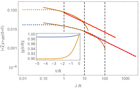
Figure 2: The response $\langle{\bar{\chi}}\chi\rangle_{\textrm{\tiny diff}}$ at fixed $t=0$ as a function of $J\delta t$ for the (one-dimensional) transverse field Ising model. The time-dependences of the coupling $g(t)$ are given in the inset. The orange curves are the log fits in the fast regime, $P\log J\delta t+Q$, and the red lines are the fits to the Kibble-Zurek scaling in the slow regime, $P^{\prime}(J\delta t)^{-1/2}+Q^{\prime}$. The dotted lines indicate expected cross-overs at $J\delta t\sim 1$ and $J\delta t\sim 1/\epsilon_{in}$. The blue dots are the response for an initial gap of $\epsilon_{in}=0.01$ and the best fits give $P=-0.00313$, $Q=0.0154$, $P^{\prime}=0.0248$ and $Q^{\prime}=5.90\times 10^{-5}$. For the yellow dots, $\epsilon_{in}=0.1$ and the best fits give $P=-0.0273$, $Q=0.0830$, $P^{\prime}=0.0777$ and $Q^{\prime}=5.10\times 10^{-4}$.

One might expect that the response will saturate when the quench is exciting all possible modes in the lattice theory, i.e., when excitations are being created in all modes. To understand this point, we begin by substituting the profile (72) (with $a=1$ and $b=\epsilon_{in}$) into the dispersion relation (24) for the Ising model and we find

$$E_{k}^{2}=4J^{2}\left[4\sin^{2}(k/2)[1+\epsilon_{in}\tanh(t/\delta t)]+\epsilon_{in}^{2}\tanh^{2}(t/\delta t)\right]\,.$$ (84)

Now we can ask when a mode at a particular wave-number $k$ is going to be excited. According to the Landau criterion (3), this mode will remain adiabatic throughout the quench (and in particular, at $t=0$) if

$$\frac{1}{E_{k}^{2}}\left|\frac{dE_{k}}{dt}\right|_{t=0}=\frac{|\epsilon_{in}|}{8J\delta t\,\sin(k/2)}\lesssim 1\,.$$ (85)

On the other hand, if the above expression exceeds one, then this mode with momentum $k$ is excited by the quench. Now it is clear that there will always be excited modes in the neighborhood of $k=0$. The above discussion may now suggest that saturation will be achieved when the violation of the above criterion (85) extends out to $k=\pi$. However, it turns out that for small amplitude quenches, only a narrow band of momenta near $k=0$ contribute significantly to the expectation value (80). In particular, we show in appendix B that $\langle{\bar{\chi}}\chi\rangle_{\textrm{\tiny diff}}$ only receives significant contributions from modes with $0\leq k<k_{max}$ with $k_{\max}=c\,|\epsilon_{in}|$ where $c$ is some order one number. Hence the violation of the criterion (85) need only extend to $k=k_{max}$ in order to produce saturation with small amplitudes. Hence it is straightforward to see from Eq. (85) that the small amplitude quenches will saturate for $J\delta t\leq 1/(4c)$ or more simply $J\delta t\lesssim 1$. Hence we have an explanation of the saturation behaviour observed for the small amplitude quenches shown in figure 2. To contrast with the following, we emphasize that the point where saturation sets in is independent of the initial amplitude here.

Now we can also examine the scaling behaviour of $\langle\bar{\chi}\chi\rangle_{\textrm{\tiny diff}}$ for “large-amplitude” quenches of the Ising model, i.e., with $|\epsilon_{in}|\gtrsim 1$. In this regime, we expect that the quenches are probing the nonlinear regime of the lattice dispersion relation (24). The response as measured by the expectation value of $\bar{\chi}\chi$ is shown for a family of four such quenches in Figure 3. These large-amplitude quenches exhibit three distinct features, which contrast with the behaviour found for the small-amplitude quenches: a) there is no longer a fast quench regime; b) the Kibble-Zurek scaling regime begins at $J\delta t\sim|\epsilon_{in}|$ (rather than $1/|\epsilon_{in}|$ for small amplitudes); and c) the response saturates to the instantaneous quench value for $J\delta t\lesssim|\epsilon_{in}|/8$ (instead of the previous $J\delta t\lesssim 1$). We now discuss each of these in somewhat more detail.

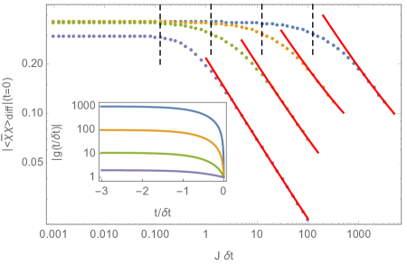
Figure 3: The response $\langle{\bar{\chi}}\chi\rangle_{\textrm{\tiny diff}}$ at fixed $t=0$ as a function of $J\delta t$ for the (one-dimensional) transverse field Ising model, for large initial amplitudes. The time-dependences of the coupling $g(t)$ are given in the inset. The red lines are the fits to the Kibble-Zurek scaling, $P(J\delta t)^{-1/2}+Q$, that starts at $J\delta t\sim|\epsilon_{in}|$. For $\epsilon_{in}=-1$, $P=0.216$ and $Q=0.00122$; for $\epsilon_{in}=-10$, $P=0.604$ and $Q=0.00984$; $\epsilon_{in}=-100$, $P=1.595$ and $Q=0.0299$; and for $\epsilon_{in}=-1000$, $P=5.247$ and $Q=0.0255$. The black dashed lines show the expected saturation point $J\delta t=|\epsilon_{in}|/8$, in each case.

The three features above are related because an essential characteristic of these large amplitude quenches is a smooth transition between the KZ and instantaneous quench regimes, without an intermediate scaling regime.. In the KZ regime, we still see scaling compatible with $\Delta=1$ expectation, i.e., $\langle\bar{\chi}\chi\rangle_{\text{diff}}\sim\delta t^{-1/2}$, while the response is saturated in the instantaneous regime. Recall that the origin of the fast quench scaling (13), is that the quench activates a growing number of short wavelength modes as $\delta t$ shrinks, but further that these new modes are organized as in a CFT dgm1 ; dgm2 . In the transition between the KZ and instantaneous quench regimes, the large amplitude quenches are already exciting modes in the nonlinear regime of the Ising dispersion relation (24), i.e., the quench is probing modes with wavelengths comparable to the lattice spacing. Hence the latter condition is not achieved in the large amplitude quenches and we should not expect to see a fast quench scaling regime.

The second important feature was that the KZ scaling sets in at a quench rate which grows with the amplitude, rather than decreasing as in the small amplitude quenches. That is, we observe that the KZ scaling begins when $J\delta t\sim|\epsilon_{in}|$ (instead of $1/|\epsilon_{in}|$) in Figure 3. This (naively) surprising behaviour can be understood by looking carefully at the conditions required for KZ scaling, as already discussed in the introduction — see the discussion around Eqs. (7) and (8). We repeat the salient points here: The first condition for our quench protocol (72) was that adiabaticity should breakdown when the profile is in the linear regime. That is, we must have $t_{KZ}<\delta t$, which in turn yields $J\delta t>1/|\epsilon_{in}|$, when expressed in terms of Eq. (7). The second condition for KZ scaling to hold was that the system has to be close to critical at $t=t_{KZ}$, i.e., $E_{KZ}<\Lambda_{\textrm{\tiny UV}}$. Interpreting $J$ as the inverse lattice spacing (see footnote 6), this condition expressed as Eq. (8) yields $J\delta t>|\epsilon_{in}|$. Of course, when $|\epsilon_{in}|$ is small, the first condition is stronger and we recover the behaviour observed in the small amplitude quenches. However, for the large amplitude quenches, it is the second restriction that determines the onset of KZ scaling, in agreement with the results found in Figure 3.

The third and final feature observed in figure 3 is that the saturation point, where the instantaneous quench regime begins, also grows with increasing amplitude in the large amplitude quenches. In fact, we observe that the expectation value saturates into the instantaneous quench value for roughly $J\delta t\lesssim|\epsilon_{in}|/8$, instead of $J\delta t\lesssim 1$ as observed for the small amplitude quenches. This behaviour can be understood by the same reasoning used above in discussing the small amplitude quenches. The key difference is that for large amplitude quenches, the response (80) does, in fact, receive significant contributions from all modes, i.e., $0\leq k\lesssim\pi$ — see appendix B for details. Hence we should ask when is the highest mode going to be excited and substituting $k=\pi$ into Eq. (85), we find

$$\frac{1}{E_{\pi}^{2}}\,\left|\frac{dE_{\pi}}{dt}\right|_{t=0}=\frac{|\epsilon_{in}|}{8J\delta t}\,.$$ (86)

Therefore all of the modes will be excited when the above expression is bigger than one, i.e., for $J\delta t\lesssim|\epsilon_{in}|/8$, and hence we expect that the expectation value will saturate in this regime for large amplitude quenches.

Finally, we should note that the quenches were studied here by measuring response exactly at the critical point. That is, we evaluated the expectation value precisely at $t=0$. One can also evaluate the response at some finite time $\tau\equiv t/\delta t$. At least for small amplitudes, the response of the continuum theory should provide a guide dgm1 ; dgm2 ; dgm3 ; dgm4 . Hence we expect that for large enough $J\delta t$, the KZ scaling regime should give way to an adiabatic regime. In fact, we expect to see this transition around $J\delta t\sim 1/(\epsilon_{in}\tau^{2})$. As shown in dgm2 , the adiabatic expansion for relativistic theories will be a series in $1/\delta t^{2}$ and hence to leading order, we expect that after subtracting the zeroth-order term for large $J\delta t$, $\langle\bar{\chi}\chi\rangle_{\text{diff}}\sim\delta t^{-2}$. We have verified that the Ising model indeed produces this behaviour. However, it is technically challenging to separate clearly all four regimes (instantaneous, fast, KZ and adiabatic) for a fixed initial amplitude and finite time.

4.2 Kitaev Honeycomb Model

Recall that to simplify our discussion of quenches in the Kitaev model (34), we restricted our attention to the subspace within the full space of couplings where $J_{1}=J_{2}=J>0$ and $J_{3}=-2J\,g$. With these restrictions, the Hamiltonian reduces to that given in Eq. (37). The critical region where the energy gap vanishes in this space of couplings reduces to the one-dimensional line segment $|g|\leq 1$, with $g=\cos{\bar{k}}$ and $k_{1}=k_{2}={\bar{k}}$ as in Eq. (38). Further, as discussed in detail in section 2.2, there are three classes of critical models: 1) interior points with $1<|g|<0$; 2) edge points with $g=\pm 1$; and 3) “interior” edge points with $g=0$; as well as the gapped phases with $|g|>1$.

As described in section 3, we quench the system with $g(t)=a+b\tanh(t/\delta t)$. In the following, we will always examine the response $\langle\bar{\chi}\chi\rangle_{\textrm{\tiny diff}}$, as defined in Eq. (80), at $t=0$. Clearly, there is a wide variety of different quenches depending on the choice of the parameters, $a$ and $b$. In particular, as we describe below, the results depend crucially on the phase in which the quench begins and on the phase at $t=0$ where we measure the response, i.e., the scaling of the responses depends on $g(t\to-\infty)=a-b$ and on $g(t=0)=a$. Of course, $\langle\bar{\chi}\chi\rangle_{\textrm{\tiny diff}}(t=0)$ will not depend on the profile of $g(t)$ at latter times $t>0$.

Given the three different types of critical theories, there are certainly a wide variety of critical quenches which one might choose to explore. In the following, we will focus on three protocols: a) ‘gapped-to-edge’ quenches which begin in the gapped phase and are measured at the edge critical point; b) ‘gapped-to-interior’ quenches which begin in the gapped phase and are measured at an interior point at some finite distance into the critical region; and c) ‘interior-to-interior’ quenches where the entire protocol only passes through interior critical points. Clearly this selection is not exhaustive and only provides a preliminary study of the critical quench dynamics of the Kitaev model — see section 5 for a discussion of other possible protocols.

One feature common to all of the different quenches is that for $J\delta t\lesssim 1$, the response saturates as a function of the quench rate. As described for the Ising model above, we can think of this as the “instantaneous quench” regime, where the quench rate is of the same order as the lattice spacing. In the discussion of the individual protocols below, we focus on the scaling of the response for the regime $J\delta t>1$. We return to consider the instantaneous quench regime in section 4.3.

4.2.1 Gapped-to-edge

Here, we consider quenches which start in the gapped phase with $g(-\infty)<-1$ and pass to the edge point with $g(0)=-1$. That is, we consider profiles (72) with $a=-1$ and $b>0$ (and hence $a-b<-1$). In this case, $b$ sets the scale of the gap in the initial phase. Further note that even though the system continues into the region of interior critical points for $t>0$, these protocols are identical to a quench from a gapped phase which crosses an isolated critical point, since a measurement at $t=0$ does not care about the values of the coupling for $t>0$.

Figure 4 shows the response for a quench with a small amplitude, i.e., $|b|\ll 1$. We see that there are two distinct scaling behaviours for $\langle{\bar{\chi}}\chi\rangle_{\textrm{\tiny diff}}(t=0)$: with exponent $-1/2$ in the fast quench regime with $1\lesssim J\delta t\lesssim 1/|b|$, and with the exponent $-3/4$ in the slow quench regime with $J\delta t\gtrsim 1/|b|$. Let us note that the scaling exponent $-3/4$ for slow quenches was also observed in earlier work hikichi , where the variation of the coupling was taken to be always linear in time and the quench was started at $t=-\infty$.

Again for small amplitudes, we expect that the quench is described well by the anisotropic continuum theory, given in Eq. (52). Recall from the discussion below Eq. (52), that the dimension of the operator $\bar{\psi}\psi$ is $\Delta=3/2$. However, the anisotropy of the theory is important to identify the fast scaling dimension. In particular, while $t$ and $y$ scale as regular coordinates with mass dimension –1, the dimension of the $x$ coordinate was –1/2. Hence the effective spacetime dimension in various formulae is $d_{\textrm{\tiny eff}}=5/2$, rather than $d=3$. For example, the dimension of ${\hat{J}}m$, the coupling conjugate to $\bar{\psi}\psi$, is $d_{\textrm{\tiny eff}}-\Delta=1$ and not $d-\Delta=3/2$. Hence using $d_{\textrm{\tiny eff}}$ in Eq. (13), we find the scaling

$$\langle\bar{\psi}\psi\rangle\sim\frac{{\hat{J}}\,m}{\delta t^{1/2}}\quad\implies\quad\langle\bar{\chi}\chi\rangle\sim\frac{b}{(J\delta t)^{1/2}}\,,$$ (87)

for fast quenches, in agreement with the results noted above and shown in figure 4. In the slow quench regime, the Kibble-Zurek time is given by $t_{KZ}=(\delta t/{\hat{J}}\,m)^{1/2}$, since in Eq. (5) $\nu=1$ and $E_{0}={\hat{J}}m$, and so the response (4) becomes

$$\langle\bar{\psi}\psi\rangle\sim\frac{1}{t_{KZ}^{\,\Delta}}=\left(\frac{{\hat{J}}\,m}{\delta t}\right)^{3/4}\quad\implies\quad\langle\bar{\chi}\chi\rangle\sim\left(\frac{b}{J\delta t}\right)^{3/4}\,.$$ (88)

Again this reproduces precisely the exponent $-3/4$ found in our numerical results.

Of course, we can also extend these quenches to large amplitudes, and as shown in figure 5, the behaviour is somewhat different. First, as expected, we do not observe any fast scaling in this case. As discussed for the Ising model above, in the transition between the instantaneous and slow quench regimes, the large amplitude quenches are probing modes with wavelengths comparable to the lattice spacing and hence they cannot be described by an effective UV CFT. Hence the fast quench scaling (13) is not produced in these large amplitude quenches. However, there does appear to be a slow scaling regime. The exponent, however, changes continuously as we increase the amplitude from $\langle\bar{\chi}\chi\rangle_{\textrm{\tiny diff}}\sim(J\delta t)^{-3/4}$ to $\langle\bar{\chi}\chi\rangle_{\textrm{\tiny diff}}\sim(J\delta t)^{-1/2}$. Of course, it will be interesting to develop an analytical understanding of this change in scaling behaviour between the small and the large amplitude quenches. This new result does not contradict the results of hikichi : in the regime where we see this scaling, the coupling is proportional to $t$ with a coefficient which is not quite small, whereas the results of hikichi refer to a regime where this coefficient is very small in units of $1/J$. Finally, in parallel to what happens in the Ising case when the amplitude is large, we see that the saturation point for small $J\delta t$ increases roughly linearly as we increase $b$.

As a final note, let us add that in the next section, we will see that for small amplitudes, the exponent for both the fast and slow quench regimes begins to change as soon as we continue the quench into the gapless phase.

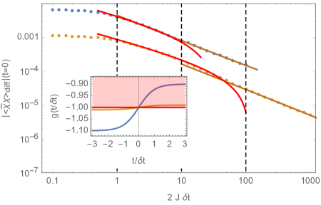
Figure 4: Plot of $\langle\bar{\chi}\chi\rangle_{\textrm{\tiny diff}}(t=0)$ as a function of $2J\delta t$ for the gapped-to-edge quench shown in the inset with $g(t)=-1+b\tanh t/\delta t$, with $b=0.1$(blue),$0.01$(yellow). The red curves are the best fit for the slow regime by a function $P+Q(2J\delta t)^{-3/4}$, where $P=-0.00448$(blue),$-0.000917$ (yellow) and $Q=-6.97\times 10^{-6}$(blue), $1.617\times 10^{-7}$(yellow). In the fast regime the brown curves indicate the best fit of a function $P+Q(2J\delta t)^{-1/2}$, with $P=-0.00499$(blue), $-9.56\times 10^{-4}$ (yellow) and $Q=0.000860$(blue), $8.96\times 10^{-5}$ (yellow).

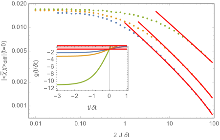
Figure 5: Plot of $\langle\bar{\chi}\chi\rangle_{\textrm{\tiny diff}}(t=0)$ as a function of $2J\delta t$ for the gapped-to-edge quench shown in the inset with $g(t)=-1+b\tanh t/\delta t$, with $b=1$(blue), $2$(yellow) and $10$ (green). The red curves are the best fit by a function $P+Q(2J\delta t)^{-1/2}$, where $P=-0.0120$(blue),$-0.0176$ (yellow), $-0.0363$ (green) and $Q=4.845\times 10^{-4}$(blue), $5.807\times 10^{-4}$(yellow), $2.322\times 10^{-4}$(green). Note also that the saturation point for small $\delta t$ increases as $b$ increases and that there is no fast scaling in the large-amplitude regime.

4.2.2 Gapped-to-interior

Next, we consider quenches where we start in the gapped phase with $g(-\infty)<-1$, pass beyond the edge point and measure the response at an interior point with $0>g(0)>-1$. That is, we are studying quench profiles (72) with $a-b<-1$ and $0>a>-1$ (and $b>0$). In this case, there are many different quench protocols that can be studied and that yield different responses. To concisely go through them, it will be convenient to define two new parameters: $\delta g_{\textrm{\tiny in}}\equiv b-a-1\ (>0)$, which sets the scale of the gap in the initial phase, i.e., measures the initial distance of $g$ to the critical region, and $\delta g_{\textrm{\tiny fin}}\equiv 1+a\ (>0)$, which measures the final distance of $g$ inside the interior critical region, i.e., , the distance of the point at which we measure the response from the edge point. There will be three clearly distinct behaviours depending on whether $\delta g_{\textrm{\tiny fin}}$ is much smaller than, greater than or the same order as $\delta g_{\textrm{\tiny in}}$.

Let us start by considering the case in which $\delta g_{\textrm{\tiny in}}>\delta g_{\textrm{\tiny fin}}$. In the previous section, we already analyzed the case where $\delta g_{\textrm{\tiny fin}}=0$, which corresponds to quenching to the edge point. In that case with small amplitudes, we found that the expectation values scale as $\delta t^{-1/2}$ in the fast regime, and $\delta t^{-3/4}$ in the slow one. Now we hold $\delta g_{\textrm{\tiny in}}$ fixed and slowly increase $\delta g_{\textrm{\tiny fin}}$ away from zero. We observe different scaling behaviours depending on whether the quench is slow or fast compared to $\delta g_{in}$, as shown in figure 6 where the initial amplitude is fixed to $\delta g_{in}=0.1$. Note that the scaling exponent in the slow quench regime, i.e., $2J\delta t>1/\delta g_{in}$, immediately changes from $-3/4$ to $-1/2$ as soon as $\delta g_{\textrm{\tiny fin}}>0$. The latter exponent corresponds to the KZ scaling of a (1+1)-dimensional fermionic mass quench. The situation is different for the fast quench regime. In this case, the scaling behaviour varies continuously from $\langle\bar{\chi}\chi\rangle_{\textrm{\tiny diff}}\sim(J\delta t)^{-1/2}$ at $\delta g_{\textrm{\tiny fin}}=0$ to a logarithmic scaling when $\delta g_{\textrm{\tiny fin}}\sim\delta g_{\textrm{\tiny in}}$.

The three examples shown in figure 6 were chosen to show the evolution of the scaling behaviour described above: The blue dots show the example where $\delta g_{\textrm{\tiny in}}=0.1$ and $\delta g_{\textrm{\tiny fin}}=0$, and hence these are quenches to the edge, as in the previous section, with a scaling exponent ${-1/2}$ in the fast regime and ${-3/4}$ in the slow regime. The yellow dots show an example where $\delta g_{\textrm{\tiny in}}=0.1$ and $\delta g_{\textrm{\tiny fin}}=0.04$. In this case, the slow quench regime already scales with an exponent $-1/2$ while the fast quench regime has an intermediate scaling (between $-1/2$ and logarithmic) with an exponent of roughly $-0.4$. The green dots correspond to quenches with $\delta g_{\textrm{\tiny fin}}=0.15\gtrsim\delta g_{\textrm{\tiny in}}=0.1$. Here, the fast quenches have already settled to a logarithmic scaling while the slow quenches again exhibit the scaling exponent $-1/2$.

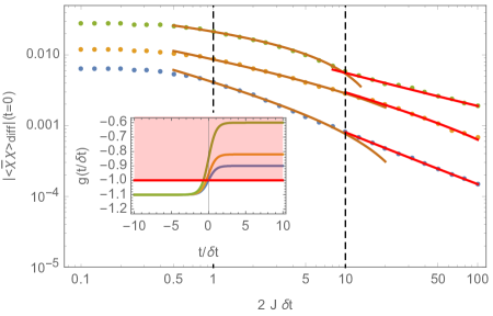
Figure 6: Plot of $\langle\bar{\chi}\chi\rangle_{\textrm{\tiny diff}}$ as a function of $2J\delta t$ for the gapped-to-gapless quenches shown in the inset. The brown and red curves are the best fits in the fast and slow quench regimes, respectively. As an example, we show here the transition between 3 different scalings. In the inset, the three quenches protocols are shown. All of them start at a distance of 0.1 from the critical region. The blue protocol goes to the edge at $t=0$, $g(t/\delta t)=-1+0.1\tanh(t/\delta t)$; the yellow protocol, just enters the critical region at $t=0$, $g(t/\delta t)=-0.96+0.14\tanh(t/\delta t)$; and the green protocol is well inside the critical area at $t=0$ (compared to the initial amplitude), $g(t/\delta t)=-0.85+0.25\tanh(t/\delta t)$. As in the previous subsection, the scalings of the blue dots correspond to the gapped-to-edge quench: in the fast regime it goes as $P+Q(2J\delta t)^{-1/2}$ (brown curve) with $P=-0.00482$ and $Q=0.000750$; in the slow regime, it behaves as $P+Q(2J\delta t)^{-3/4}$ (red curve) with $P=-0.00448$ and $Q=-6.97\times 10^{-6}$. Now, when you measure inside the critical area, the slow scaling changes instantaneously to $-1/2$, while the fast quench continually changes from $-1/2$ to a logarithmic scaling. Thus, the two regimes in the yellow quench are given by $P+Q(2J\delta t)^{-\alpha}$ (brown, fast), with $P=-0.00963,Q=0.000884,\alpha=0.406$ and $P+Q(2J\delta t)^{-1/2}$ (red, slow), with $P=-0.0107$,$Q=0.000439$. Finally, the green curve shows the prototypical example of a gapped-to-interior quench with best fits $P+Q\log(2J\delta t)$ (brown, fast), with $P=0.00690$, $Q=-0.0213$ and $P+Q(2J\delta t)^{-1/2}$ (red, slow), with $P=-0.0170$ and $Q=-0.000200$.

In figure 7, we explore the transition between the edge scaling to logarithmic scaling in the fast quench regime. We analyze different quench protocols, all with fixed $\delta g_{\textrm{\tiny in}}=0.1$ and with $\delta g_{\textrm{\tiny fin}}$ varying from $0$ to $0.15$ — see figure 7a. In figure 7b, we show the corresponding scaling exponent in the fast quench regime fit with $\langle\bar{\chi}\chi\rangle_{\textrm{\tiny diff}}\sim(J\delta t)^{-\alpha}$. We see that the exponent $\alpha$ begins at 1/2 and smoothly decreases until some value just below $0.1$ when $\delta g_{\textrm{\tiny fin}}\sim 0.1$ At this point, $\alpha$ saturates for large $\delta g_{\textrm{\tiny fin}}$. In fact, the scaling of the expectation value has become logarithmic, but it turns out that this is indistinguishable from power-law scaling with the small exponents shown in the figure.

In summary, the (small amplitude) quenches from the gapped phase to the interior of the critical region exhibit two scaling regimes: The slow quench regime with $2J\delta t>1/\delta g_{\textrm{\tiny in}}$ where $\langle\bar{\chi}\chi\rangle_{\textrm{\tiny diff}}$ always scales as $(J\delta t)^{-1/2}$ for any $\delta g_{\textrm{\tiny fin}}>0$, which is distinct from $(J\delta t)^{-3/4}$ scaling observed with $\delta g_{\textrm{\tiny fin}}=0$. We might add that this behaviour would be the KZ scaling for a (1+1)-dimensional fermionic theory. In the fast quench regime with $2J\delta t<1/\delta g_{\textrm{\tiny in}}$, the scaling behaviour makes a smooth transition from the quench-to-edge scaling of $(J\delta t)^{-1/2}$ to a logarithmic scaling, that would be expected for a (1+1)-dimensional fermionic mass quench. This transition occurs over the range $0<\delta g_{\textrm{\tiny fin}}\lesssim\delta g_{\textrm{\tiny in}}$.

Now it is natural to ask whether the same scaling holds for large amplitude quenches inside the critical region, i.e., for quenches with $\delta g_{\textrm{\tiny fin}}\gtrsim\delta g_{\textrm{\tiny in}}$. These large amplitude quenches are explored in figure 8. As the whole region on interior critical points is traversed with $\delta g_{\textrm{\tiny fin}}=1$ to analyze larger amplitudes, we need to start with smaller $\delta g_{\textrm{\tiny in}}$. For the quenches shown in figure 8, we fix $\delta g_{\textrm{\tiny in}}=0.01$ and vary the final amplitude $\delta g_{\textrm{\tiny fin}}=0.1,0.25,0.45,0.75$, all of which satisfy $\delta g_{\textrm{\tiny fin}}\gg\delta g_{\textrm{\tiny in}}$. In this large amplitude regime, the corresponding fast and slow quench scalings remain the same as above, i.e., $-1/2$ and logarithmic, respectively. However, now the transition between the two scaling regimes is no longer at $2J\delta t\sim 1/\delta g_{\textrm{\tiny in}}=100$, rather we find the transition at $2J\delta t\sim\delta g_{\textrm{\tiny fin}}$. In fact, we see that as $\delta g_{\textrm{\tiny fin}}$ increases and becomes of order one, the fast quench scaling regime shrinks more and more until is no longer observable, as shown with the violet dots in figure 8 which predominantly scale with the slow quench scaling.

Another alternative approach to large amplitude quenches is to consider quenches where we fix $\delta g_{\textrm{\tiny fin}}$ but we increase the gapped amplitude $\delta g_{\textrm{\tiny in}}$. We followed this approach with $\delta g_{\textrm{\tiny fin}}=0.1$ fixed and varying $\delta g_{\textrm{\tiny in}}=0.1,1,10,100$. When both $\delta g$’s are comparable, we found the same result as before; namely, a logarithmic fast scaling regime and a power-law slow regime with exponent $-1/2$, separated at a scale $\delta g_{\textrm{\tiny in}}^{-1}\sim\delta g_{\textrm{\tiny fin}}^{-1}$. As we increased $\delta g_{\textrm{\tiny in}}$, the logarithmic scaling remains but the exponent of the power-law starts decreasing, until around $\delta g_{\textrm{\tiny in}}=10$, where we can only observe a logarithmic behaviour. This is a rather surprising behaviour, given that in every other case the fast scaling was the regime which disappeared for large amplitudes. One possibility is that there is indeed still a slow quench regime (which sets in at some scale given by a combination of $\delta g_{\textrm{\tiny in}}$ and $\delta g_{\textrm{\tiny fin}}$) that will only appear for large enough $J\delta t$.

We do not have a good understanding of the various scaling behaviours described above. The scaling exponent of $-1/2$ in the slow quench regime has been observed previously for quenches linear in time for this model sengupta . These linear quenches began at $t=-\infty$ and the response is measured at $t=+\infty$. With these simple protocols, the response can be examined analytically and the $1/(J\delta t)^{1/2}$ scaling stems from the fact that the excitation probability predominantly depends on one of the directions in momentum space. Recall that the critical models (41) for the interior points are not really anisotropic and so we expect that this result must be related to the fact that the quenched operator itself is anisotropic. That is, from the critical Hamiltonian in Eq. (44), we see that the quenched operator corresponds to $\bar{\psi}\gamma_{x}\psi$. Hence we should think of $m(t)$ as the $x$-component of a vector coupling and accordingly, the roles of $p_{x}$ and $p_{y}$ are clearly distinguished in the dispersion relation (45) — see further discussion in section 5. Of course, for the protocols used in this paper, our numerical results exhibit a behaviour similar to that in the linear quenches, as long as the gapless interior region is traversed, irrespective of the starting point.

(a) Quenches Protocols

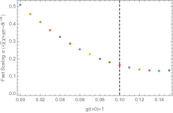
(b) Resulting scaling in the fast regime

Figure 7: Resulting scaling in the fast regime as a function of how deep inside the critical region it is measured. For the quench to the edge, it is expected a fast scaling of $\delta t^{-1/2}$ (see last subsection). That scaling slowly decays until it stabilizes when the distance inside the critical region is of the order of the initial amplitude (in this case, 0.1). At that stage (shown in dashed black line), the scaling of the expectation value becomes logarithmic, that in figure (b) is presented as a “small” power-law behaviour.

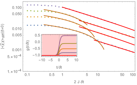
Figure 8: Plot of $\langle\bar{\chi}\chi\rangle_{\textrm{\tiny diff}}$ as a function of $2J\delta t$ for the large-amplitude gapped-to-gapless quenches shown in the inset. The initial distance to the critical region is 0.01. The brown and red curves are the best fits in the fast and slow quench regimes, respectively. In all cases they correspond to fits by $P_{1}+Q_{1}\log(2J\delta t)$ for the fast and $P_{2}+Q_{2}(2J\delta t)^{-1/2}$ for the slow regime. $P_{1}=0.00385$ (blue), $0.0119$ (yellow), $0.0240$ (green); $Q_{1}=-0.0115$ (blue),$-0.0291$ (yellow), $-0.0544$ (green); $P_{2}=-0.00857$ (blue),$-0.0229$ (yellow), $-0.0448$ (green), $-0.110$ (violet); $Q_{2}=0.0000391$(blue), $0.000421$ (yellow), $0.000443$ (green), $0.00194$ (violet). The crossover between fast and slow regimes happens at a $J\delta t$ that is inversely proportional to the amplitude of the quench, making the fast regime to effectively disappear when the amplitude is large enough (like for the violet dots).

For slow quenches, the change of the exponent from 3/4 to 1/2 as soon as $\delta g_{in}\neq 0$ may be understood as follows: Consider first the line $k_{1}=k_{2}={\bar{k}}$, so that $G(k)=0$. In this case the equations for $\chi_{1}$ and $\chi_{2}$, as defined in equation (62), decouple. The solutions of the Dirac equation can be readily written down

$$\chi_{1}({\bar{k}}) = A_{1}\,{\rm exp}[-i\alpha({\bar{k}},t)]\,,$$

$$\chi_{2}({\bar{k}}) = A_{2}\,{\rm exp}[i\alpha({\bar{k}},t)]\,,$$ (89)

where $A_{1},A_{2}$ are integration constants and

$$\alpha({\bar{k}},t)=-\int^{t}m({\bar{k}},t^{\prime})dt^{\prime}=-4J[(a-\cos{\bar{k}})t+b\delta t\log(\cosh t/\delta t)]\,.$$ (90)

To determine the “in” solution, we need to examine the behavior at $t\rightarrow-\infty$,

$$\alpha({\bar{k}},t)\rightarrow-4J(a-b-\cos{\bar{k}})t\,.$$ (91)

Since we are considering quenches which start from the gapped phase we have $(a-b)<-1$, so that $(a-b-\cos{\bar{k}})<0$. Therefore for the positive energy solution we must set $A_{2}=0$, while for the negative energy solution we must set $A_{1}=0$,

$$U({\bar{k}},t)=A_{1}\left(\begin{array}[]{c}e^{-i\alpha({\bar{k}},t)}\\ 0\end{array}\right)\,,$$ (94)

$$V({\vec{k}},t)=A_{2}\left(\begin{array}[]{c}0\\ e^{i\alpha({\bar{k}},t)}\end{array}\right)\,.$$ (97)

Substituting these in the mode expansion for the operator $\chi$ as in eq. (76) and imposing the anticommutation relations then determines the integration constants $A_{1}=A_{2}=1$ upto a phase.

Therefore for these $k_{1}=k_{2}={\bar{k}}$ modes, we have

$${}_{in}\langle 0|{\bar{\chi}}\chi|0\rangle_{in}={\bar{V}}({\vec{k}},t)V({\vec{k}},t)=-1\,,$$ (98)

which is independent of ${\vec{k}}$ and time.

Consider now the response which we measure, viz. the quantity $\langle{\bar{\chi}}\chi\rangle_{\textrm{\tiny diff}}$ defined in eq. (80). The adiabatic modes at time $t=0$ for $k_{1}=k_{2}={\bar{k}}$ are

$$\chi_{1}^{adia}({\bar{k}}) = A_{1}\,{\rm exp}[i\,m({\bar{k}},0)t]\,,$$

$$\chi_{2}^{adia}({\bar{k}}) = A_{2}\,{\rm exp}[-i\,m({\bar{k}},0)t]\,,$$ (99)

Therefore the negative frequency adiabatic modes have $\chi_{1}=0$ when $m({\bar{k}},0)<0$ while they have $\chi_{2}=0$ when $m({\bar{k}},0)>0$. Therefore we have

$${}_{in}\langle 0|{\bar{\chi}}({\vec{k}})\chi({\vec{k}})|0\rangle_{in} = -1~{}~{}~{}~{}(m({\bar{k}},0)<0)\,,$$ (100)

$$= +1~{}~{}~{}~{}(m({\bar{k}},0)>0)\,.$$

which subsequently means that

$$\langle{\bar{\chi}}({\vec{k}})\chi({\vec{k}})\rangle_{\textrm{\tiny diff}} = \ 0\qquad\ (m({\bar{k}},0)<0)\,,$$ (101)

$$= -2\qquad(m({\bar{k}},0)>0)\,.$$

Let us now consider quench protocols “gapped to edge”. These have $a=-1$ and $b>0$. This means $m({\vec{k}},0)=-4J(\cos{\vec{k}}-a)=-8J\cos^{2}({\vec{k}}/2)\leq 0$ for these quenches, so that $\langle{\bar{\chi}}({\vec{k}})\chi({\vec{k}})\rangle_{\textrm{\tiny diff}}=0$. On the other hand for quench protocols “gapped to interior”, we need $a=-1+2\eta$ where $\eta>0$, so that $m({\vec{k}},0)=-8J(\cos^{2}{\bar{k}}/2-\eta)$. This can be positive for ${\vec{k}}$ such that $\cos^{2}{\bar{k}}/2<\eta$.

We therefore conclude that along the $k_{1}=k_{2}={\bar{k}}$ the contribution to the response, $\langle{\bar{\chi}}({\vec{k}})\chi({\vec{k}})\rangle_{\textrm{\tiny diff}}$ is always independent of ${\vec{k}}$. This vanishes for all ${\vec{k}}$ for gapped to edge quenches, whereas for gapped to interior quenches there is a range of ${\vec{k}}$ for which this has the maximal value $-2$.

Consider now the response for generic $k_{1}$ and $k_{2}$. The components $\chi_{1},\chi_{2}$ satisfy the equation

$$\left[\partial_{t}^{2}\pm i\partial_{t}m({\vec{k}},t)+[G({\vec{k}})^{2}+m({\vec{k}},t)^{2}]\right]\chi_{1.2}=0\,.$$ (102)

For slow quenches the response is substantial for times when the quench profile can be approximated by a profile which is linear in time. For these times, eq. (102) becomes

$$\left[\partial_{t}^{2}\pm i4Jb/\delta t+[G({\vec{k}})^{2}+m({\vec{k}},t)^{2}]\right]\chi_{1,2}=0\,.$$ (103)

Rescaling $t\rightarrow t^{\prime}=t/\sqrt{\delta t}$ it is clear that solutions have a functional form

$$\chi_{1,2}=F(G({\vec{k}})\sqrt{\delta t},m({\vec{k}},t)\sqrt{\delta t},t/\sqrt{\delta t})\,.$$ (104)

This, in turn, implies that the quantity $\langle{\bar{\chi}}({\vec{k}})\chi({\vec{k}})\rangle_{\textrm{\tiny diff}}$ also has this functional form.

Since we have shown that this quantity is independent of momenta when $G(k)=0$, the simplest form of this function at time $t=0$ is

$$\langle{\bar{\chi}}(k)\chi(k)\rangle_{\textrm{\tiny diff}}=c_{1}\,F_{1}(G({\vec{k}})\sqrt{\delta t})+c_{2}\,(G(k)\sqrt{\delta t})^{\alpha}\,F_{2}(G({\vec{k}})\sqrt{\delta t},m({\vec{k}},t)\sqrt{\delta t})+\cdots\,,$$ (105)

where $F_{1,2}$ are some functions and $\alpha$ is some positive real exponent. The ellipsis indicates higher orders in $G({\vec{k}})\sqrt{\delta t}$.

For gapped-to-edge quenches, we have also shown that $\langle{\bar{\chi}}({\vec{k}})\chi({\vec{k}})\rangle_{\textrm{\tiny diff}}$ vanishes for all ${\vec{k}}$. Therefore for such quenches, the first term must be absent, or we should set $c_{1}=0$. On the other hand, for gapped-to-interior quenches, $\langle{\bar{\chi}}({\vec{k}})\chi({\vec{k}})\rangle_{\textrm{\tiny diff}}$ is nonvanishing for some range of momenta. Therefore for such quenches the first term is generically nonvanishing.

Since we are considering slow quenches, most of the contribution will come from the region in momentum space where $G(k)$ is small. In this region we can approximate

$$G(k)\sim 2k_{-}\cos(k_{+})\,,$$ (106)

where $k_{\pm}=\frac{1}{2}(k_{1}\pm k_{2})$. Thus, for gapped-to-interior quenches, we have

$$\langle{\bar{\chi}}\chi\rangle_{\textrm{\tiny diff}}=\int dk_{+}dk_{-}F_{1}(\cos k_{+}(k_{-}\sqrt{\delta t}))\sim(\delta t)^{-1/2}\,.$$ (107)

On the other hand, for gapped-to-edge quenches, most of the contribution should come from the single gapless point which has $k_{+}=\pi,k_{-}=0$. Expanding around this point, $k_{+}=\pi+\delta k_{+}$ and $k_{-}=\delta k_{-}$ where both $\delta k_{\pm}$ are small we have

$$G(k)\sim-2\delta k_{-}~{}~{}~{}~{}~{}m(k,0)\sim(\delta k_{+})^{2}+(\delta k_{-})^{2}\,.$$ (108)

Therefore, we have

$$\langle{\bar{\chi}}\chi\rangle_{\textrm{\tiny diff}}=\int d\delta k_{+}d\delta k_{-}(\delta k_{-}\sqrt{\delta t})^{\alpha}F_{2}(\delta k_{-}\sqrt{\delta t},(\delta k_{+}^{2}+\delta k_{-}^{2})\sqrt{\delta t})\,.$$ (109)

To extract the leading $\delta t$ dependence we rescale $\delta k_{-}\rightarrow\delta k_{-}\sqrt{\delta t}$ and $\delta k_{+}\rightarrow\delta k_{+}(\delta t)^{1/4}$ to get

$$\langle{\bar{\chi}}\chi\rangle_{\textrm{\tiny diff}}\sim(\delta t)^{-3/4}\,.$$ (110)

4.2.3 Interior-to-interior

In this section, we consider quenches where both $g(-\infty)$ and $g(0)$ are at interior critical points — and in fact, where the entire protocol from $t=-\infty$ to 0 passes only through interior points. That is, we consider profiles (72) with $-1<a<0$ and $-1<a-b<0$ (as well as $b>0$).

Typical results are shown in figure 9 where we consider two different protocols one with $b=0.1$ and the other with $b=0.01$. One somewhat surprising feature is that we, in fact, observe two different scaling regimes, separated at a scale of $J\delta t$ of the order of the inverse of the amplitude, i.e., $J\delta t\sim 1/b$, even though the quench only travels across interior critical points at all times. The two scaling regimes are characterized by distinct scaling exponents. For $1<J\delta t<1/b$, we found that expectation values scale as $1/(J\delta t)$, which is consistent with the fast scaling of a (2+1)-dimensional fermionic mass quench. On the other hand, in the slow regime where $J\delta t>1/b$, we find $\langle\bar{\chi}\chi\rangle_{\textrm{\tiny diff}}\sim(J\delta t)^{-1/2}$, which matches the slow quench scaling found for gapped-to-interior quenches in the previous section.

Of course, since the amplitudes considered in Figure 9 are still small, it would be very interesting to develop an understanding of these scalings in terms of a continuum theory described in section 2.2. In particular, there is a striking fact to understand, namely, why is there a slow quench regime at all? Since the quench only passes through interior points where the model is gapless, there is no intrinsic energy scale with which to compare the quench rate, i.e., the quenches are never in an adiabatic regime, no matter how large $J\delta t$ becomes. We checked this last fact by computing expectation values at a finite time but never observing an adiabatic evolution. However, the numerical computations still show that there is a slow scaling regime for these quenches, which therefore cannot be adiabatic and somehow the scaling exponent matches the KZ scaling for a mass quench in $(1+1)$-dimensional fermionic theory! We also reiterate that this behaviour also matches the slow quench scaling found for gapped-to-interior quenches in the previous section. There it was suggested that this unusual scaling was associated with the anisotropy of the quenched operator.

One observation, which provides a step towards a possible explanation, is the following: In dgm1 ; dgm2 , it was shown that the fast quench scaling behaviour essentially follows from linear response theory. In our case, the dimensionless parameter which controls the renormalized perturbation theory is $Jb\,\delta t$. Thus the linear response would be valid when $Jb\,\delta t$ is small, and indeed in this regime, we get the expected result from the continuum theory. That is, we find the fast quench scaling, i.e., $1/(J\delta t)$, for a mass quench in a (2+1)-dimensional fermionic theory. On the other hand, when $Jb\,\delta t>1$, the linear response calculation is no longer valid, and the arguments which lead to the fast quench scaling do not hold any more. Indeed the change of the scaling exponent changes precisely around $Jb\,\delta t\sim 1$. While this does not explain the new scaling $(J\delta t)^{-1/2}$ found beyond this point, it does indicate that we should expect that the quenches are entering a new regime here.

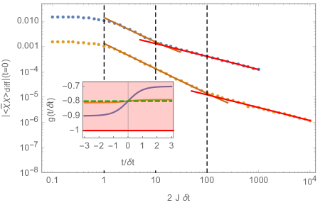
Figure 9: Plot of $\langle\bar{\chi}\chi\rangle_{\textrm{\tiny diff}}$ as a function of $2J\delta t$ for the interior-to-interior quench. The quench protocols are shown in the inset with $g(t/\delta t)=-0.8+b\tanh t/\delta t$, where $b=0.1$ (blue), $0.01$ (yellow). The green dashed line shows the value at which we are computing, $g(t=0)=-0.8$. The shaded red area is critical. The red fits are for functions $P(2J\delta t)^{-1/2}+Q$ with $P=-0.00416,1.22\times 10^{-4},Q=1.01\times 10^{-5},7.60\times 10^{-8}$, respectively. The brown curves show the best fit for functions $P(2J\delta t)^{-1}+Q$ with $P=0.0139,-0.00131,Q=1.42\times 10^{-4},6.04\times 10^{-7}$.

4.3 Instantaneous quench limit

Irrespective of the particular model under consideration, when the quench rate is faster than the lattice scale, i.e., $J\delta t\lesssim 1$, we expect that our results should agree with that of an instantaneous quench in which the coupling is switched abruptly from $g(t=-\infty)$ to $g(t=0)$ at the time of measurement. In particular, the system has no time to respond to the change in the coupling and so to a good approximation, we have

$${\rm instantaneous\ quench:}\ \ \ \langle\bar{\chi}\chi\rangle_{\textrm{\tiny diff}}=\langle\bar{\chi}\chi\rangle_{\textrm{\tiny adia}}\big{|}_{t=-\infty}-\langle\bar{\chi}\chi\rangle_{\textrm{\tiny adia}}\big{|}_{t=0}\,.$$ (111)

Hence given the expression for $\langle\bar{\chi}\chi\rangle_{adia}(t)$ in Eq. (83), it is straightforward to calculate $\langle\bar{\chi}\chi\rangle_{\textrm{\tiny diff}}$ for this regime.

For the Kitaev model, Eq. (83) yields

$$\langle\bar{\chi}\chi\rangle_{\textrm{\tiny adia}}(t)=-\int_{0}^{\pi}\int_{0}^{\pi}\frac{dk_{1}dk_{2}}{(2\pi)^{2}}\,\frac{\cos k_{1}+\cos k_{2}-2g(t)}{\sqrt{(\cos k_{1}+\cos k_{2}-2g(t))^{2}+(\sin k_{1}-\sin k_{2})^{2}}}\,.$$ (112)

Now as an example, figure 10 shows the result for $\langle\bar{\chi}\chi\rangle_{\textrm{\tiny diff}}$ at $t=0$ for a quench protocol which starts in the gapped phase with $g(t=-\infty)=-1.01$, and ends in the interior of the critical region with $g(t=0)=-0.9$. The figure also shows the instantaneous quench result (111) evaluated with Eq. (112). The figure clearly shows that in the limit $J\delta t\rightarrow 0$, the exact numerical results smoothly approach the instant quench value (111). Similarly, we have verified that the saturation value of $\langle\bar{\chi}\chi\rangle_{\textrm{\tiny diff}}$ agrees with Eq. (111) in the Ising model.

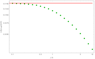
Figure 10: Plot of $\langle\bar{\chi}\chi\rangle_{\textrm{\tiny diff}}$ at $t=0$ as a function of $J\delta t$ for the gapped-interior quench shown in the inset. At the beginning of the quench $g(t=-\infty)=1.01$ and we measure at $g(t=0)=0.9$. The red line is the result (111) for instantaneous quenches evaluated using Eq. (112), which in this case yields $0.0155$.

Beyond $t=0$

The exact result for an instantaneous quench in the Ising model from a coupling $g=g_{0}$ to $g=g_{1}$ was calculated in barouch ,

$$\langle\bar{\chi}\chi\rangle_{\textrm{\tiny inst}}(t) = \int_{0}^{\pi}\frac{dk}{\pi\,\epsilon_{0}(k)\,\epsilon_{1}^{2}(k)}\,\Big{[}(g_{0}-g_{1})\sin^{2}k~{}\cos(2\epsilon_{1}t)$$ (113)

$$\qquad-(\cos k-g_{1})\big{(}(\cos k-g_{0})(\cos k-g_{1})+\sin^{2}k\big{)}\Big{]}\,,$$

where

$$\epsilon_{i}=\Big{(}\sin^{2}k+(g_{i}-\cos k)^{2}\Big{)}^{1/2}\,.$$ (114)

Hence in the Ising model, we can compare our full solution $\langle\bar{\chi}\chi\rangle(t)$ for quench rates faster than the lattice scale with this instantaneous quench answer, for all times $t>0$. In Figure (11), we compare the time dependence of ${}_{in}\langle 0|{\bar{\chi}}\chi|0\rangle_{in}$ at small values of $\delta t$ with the exact instant quench result Eq. (113) and we see that the agreement gets better as $J\delta t$ decreases.

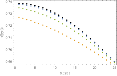
Figure 11: Comparison of the instantaneous quench answer (black dots) in Eq. (113) with the time-dependent solution for $J\delta t=0.5$ (orange dots), $J\delta t=0.25$ (green dots) and $J\delta t=0.1$ (blue dots).

5 Discussion

In this paper, we have studied critical quench dynamics in the transverse field Ising model (23) on one-dimensional chain and in the Kitaev honeycomb model (34) in two dimensions. We studied an exactly solvable quench protocol which asymptotes to finite values of the coupling at early and late times, and focused on the response of the operator by which we carried out the quench. The exact solutions in terms of free fermions were used to study the scaling of the response with the quench rate. Our answers have been obtained in the thermodynamic limit with an infinite number of sites and thus are free from finite size effects. Our results are summarized in Table 3.

Theory		Slow	Fast	Transition
Continuum Free Fermion	$d=1+1$	1/2	$\log$	$m_{0}^{-1}$
	$d=2+1$	1	1	$m_{0}^{-1}$
Transverse Ising Model	small amplitude; $\epsilon_{in}\ll 1$	1/2	$\log$	$\epsilon_{in}^{-1}$
	large amplitude; $\epsilon_{in}\gg 1$	1/2	none	$\epsilon_{in}$
Kitaev Honeycomb Model	gapped-to-edge
	small amplitude; $b\ll 1$	3/4	1/2	$|b|^{-1}$
	large amplitude; $b\gg 1$	1/2	none	$|b|\$
	gapped-to-interior
	$\delta g_{\textrm{\tiny in}}\gg\delta g_{\textrm{\tiny fin}}$	1/2	$\frac{1}{2}>\alpha>0$	$\delta g_{\textrm{\tiny in}}^{-1}$
	$\delta g_{\textrm{\tiny in}}\sim\delta g_{\textrm{\tiny fin}}$	1/2	$\log$	$\delta g_{\textrm{\tiny in}}^{-1}$
	$\delta g_{\textrm{\tiny in}}\ll\delta g_{\textrm{\tiny fin}}$	1/2	$\log$	$\delta g_{\textrm{\tiny fin}}^{-1}$
	interior-to-interior	1/2	1	$|b|^{-1}$

Table 3: A summary of our results for the scaling behaviour in critical quenches of the transverse field Ising model (23) and the Kitaev honeycomb model (34). We have also included the analogous results for a free fermion in two and three dimensions, for comparison. The columns ‘Slow’ and ‘Fast’ indicate the scaling exponent in the response, i.e., $\langle{\bar{\chi}}\chi\rangle_{\textrm{\tiny diff}}\sim(J\delta t)^{-\alpha}$, for the slow and fast quench regimes — ‘log’ indicates a logarithmic scaling was found and ‘none’ indicates the fast scaling regime disappears. The column ‘Transition’ indicates the approximate value of $J\delta t$ when the scaling makes a transition between the two scaling regimes, or the minimum value for the slow scaling when there is no fast scaling regime. For the continuum free fermion, we are indicating the value of $\delta t$ at this transition.

The results for the Ising model, discussed in section 4.1, are the ones which are best understood. The Ising model has an isolated critical point. Our quench protocol takes us through this point and we measure the response at the moment (chosen to be $t=0$) when the quench hits the critical point. For small amplitude quenches (with $\epsilon_{in}=b\ll 1$), there are three different regimes, as shown in figure 2: 1) for $J\delta t\lesssim 1$, the response saturates and we are in the instantaneous quench regime; 2) for $1\lesssim J\delta t\lesssim 1/\epsilon_{in}$, the response scales logarithmically with $J\delta t$, as expected from the continuum description of the fast quench regime; and 3) for $J\delta t>1/\epsilon_{in}$, the response scales as $1/(J\delta t)^{1/2}$, as expected for Kibble-Zurek scaling in continuum. Hence for quenches which only make small excursions from the critical point, our results agree with those expected for the continuum theory dgm1 ; dgm2 ; dgm3 ; dgm4 . However, we can also consider large amplitude quenches (with $\epsilon_{in}=b\gtrsim 1$) and the scaling behaviour changes in this regime. In particular, the fast quench scaling regime disappears and rather there is a smooth crossover between the instantaneous and slow quench regimes. Further, the slow scaling behaviour matches the KZ scaling found above, but the transition into this regime occurs roughly when $J\delta t\sim\epsilon_{in}$.

As described in section 4.1, for the Ising model, we have a good theoretical understanding of the response in all of the different situations described above. Perhaps one of the most interesting results here is that there is a fast scaling regime for small amplitude quenches. That is, our analysis of the Ising model confirms that even with a finite lattice spacing, certain quench protocols produce the fast scaling behaviour originally discovered in the study of continuum field theories numer ; fastQ ; dgm1 ; dgm2 — see further discussion below.

The Kitaev model is distinguished by having an extended region of couplings for which the theory is gapless. In section (4.2), we considered a variety of different quench protocols with different starting points and measuring the response at different points in the critical region (again, chosen to be time $t=0$), and the results are summarized in Table 3.

The simplest case to consider is the gapped-to-edge quench, described in section 4.2.1, where the quench of the Kitaev model starts in the gapped phase and at $t=0$, the system is at the edge of the gapless region. The situation here is very similar to that of quenching across an isolated critical point, as in the Ising model. Indeed for small amplitude quenches, we observe three distinct scaling regimes: instantaneous, fast and slow regimes, which can be understood in terms of the continuum model (52). However, we must add that the latter is an anisotropic theory and the scaling behaviour does not match the scaling of a conventional fermionic field, which is also shown in Table 3. Further, for large amplitude quenches, the fast scaling regime disappears. One difference in the Kitaev case is that for the large amplitude quenches, the scaling exponent in the slow regime is different from that in the small amplitude quenches.

We began to explore the extended critical region of the Kitaev model with the gapped-to-interior and interior-to-interior quenches, which are discussed in sections 4.2.2 and 4.2.3. In both cases, the response is measured when the system is at an interior critical point, while in the first family, the quench starts in the gapped phase and in the second, the system is initially at an interior point. For all of these quenches, we again observe three distinct scaling regimes: slow, fast and instantaneous, with smooth transitions between them. The scaling behaviour in the fast regime depends on the details of the quench, as shown in Table 3. However, for all of these quenches which traverse a finite part of the critical region, all exhibit the same scaling exponent in the slow quench regime. Namely, $\langle{\bar{\chi}}\chi\rangle_{\textrm{\tiny diff}}\sim(J\delta t)^{-1/2}$, which corresponds to the Kibble Zurek scaling of a relativistic fermion in one lower dimension. In fact, our preliminary results indicate this slow scaling behaviour extends to any quenches which traverse some distance in the interior region, e.g., quenches beginning at an interior point and ending at an edge point or vice versa.

This slow quench behaviour has been observed earlier for quenches of the Kitaev model with linear protocols which start at $t=-\infty$, and the measurement is performed at $t=\infty$ sengupta . In this case, the equivalent Landau-Zener problem has a simple solution and for slow quench rates, the excitation probability predominantly depends on $k_{y}$ alone. We do not have a clear explanation for how this behaviour emerges with our quench protocols at the moment. However, examining the integrand $\langle\bar{\chi}\chi\rangle(\vec{k})$ in an expansion around the critical modes, we find that this quantity depends primarily on $k_{y}=k_{1}-k_{2}$ and is almost independent of $k_{x}=k_{1}+k_{2}$. Hence this momentum dependence reflects the same behaviour found for the excitation probability for the linear quenches sengupta . Further, as commented in section 4.2.2, while the critical models (41) for the interior points are not anisotropic, these quenches are inherently anisotropic because the quenched operator corresponds to $\bar{\chi}\gamma_{x}\chi$. Accordingly, we should think of coupling which we are varying in the quenches as the $x$-component of a vector. We expect that this anisotropy will play a central role in the explanation of the unusual scaling found in both the slow and fast quench regimes.

As commented above, one of the most interesting results here is that there is a fast scaling regime in many of our lattice quenches. For small amplitudes, our numerical results here match to the expectations of a continuum analysis for the Ising model and for the gapped-to-edge quenches in the Kitaev model. While we presently lack a theoretical understanding, it also appears that a fast scaling regime arises for quenches of the Kitaev model which traverse a finite distance across the critical region, e.g., for the gapped-to-interior and interior-to-interior quenches. Therefore our results indicate that for systems with a finite lattice spacing, there is quite generally a regime where the quench rates lie between the inverse lattice spacing and the physical mass scales, and where the fast scaling behaviour found previously only in continuum field theories holds. This opens up the interesting possibility that such scaling can be indeed observed in experiments.

In the cases where we can match the theoretical and numerical analysis for the fast scaling regime, the dimensionless couplings are small and the change in the couplings are small as well. It is only in this case that the crossover from the fast to the slow quench happens when $\delta t$ is of the order of the inverse physical mass scale. This is expected, since small dimensionless couplings correspond to finite physical mass scales and the continuum fast quench scalings are expected when the quench rate is fast compared to the physical scales but slow compared to the UV cutoff scale. Indeed, in the case of the Ising model, when $\Delta g(t)\sim{\cal O}(1/|m_{in}|)$ and in the case of the Kitaev quench from gapped to the edge for $\Delta J_{3}(t)\sim{\cal O}(1/|m_{in}|)\sim{\cal O}(1/J)$ we still have three regimes, but now the crossover between the fast and the slow regime is no longer at $\delta t\sim 1/|m_{in}|$. On the other hand the slow quench behaviour is insensitive to this, since this is the regime where the physical mass scale is much higher than the scale set by the quench rate.

There are a wide variety of different avenues to follow in extending our study of critical quench dynamics in lattice models. In particular, the three protocols introduced in section 4.2 to study the Kitaev model do not form an exhaustive list of the possibly interesting quench protocols in this lattice model. As alluded to in the above discussion, we have made some preliminary studies of interior-to-edge and edge-to-interior quenches. One feature that seems to extend to these protocols is the slow quench scaling: $\langle{\bar{\chi}}\chi\rangle_{\textrm{\tiny diff}}\sim(J\delta t)^{-1/2}$. It also appears that there is a fast scaling regime separating the instantaneous and slow quench regimes. As noted in section 2.2, there is a distinct “interior” edge point with $g=0$. It would be interesting to probe this new critical theory with new quench protocols.

From the quantum information perspective, it will be important to understand quench dynamics on the open chain Cluster-Ising model which has non-trivial symmetry protected edge-states — see appendix C. In that context, it will be interesting to study the response of the string order parameter cluster-ising , in a similar manner in terms of free fermions.

As we commented above, the quenches in the Kitaev model which traverse the critical region are inherently anisotropic. While the critical theories corresponding to the interior critical points are not anisotropic, we are quenching the system with an anisotropic operator, i.e., $\chi^{\dagger}\sigma_{3}\chi\sim\bar{\chi}\gamma_{x}\chi$ (in the continuum langauge). We also measure the response as the expectation value of this same operator. Hence it would be interesting to see if similar scaling laws hold in these quenches for other operators like $\chi^{\dagger}\sigma_{1}\chi$, $\chi^{\dagger}\sigma_{2}\chi$ or $\chi^{\dagger}\chi$. Undoubtedly, this would give us new insights into the unusual scaling behaviour found for, e.g., the gapped-to-interior and interior-to-interior quenches.

Of course, we do not have a good theoretical understanding of many results for the quenches in the Kitaev model, particularly, for quenches that traverse a finite distance in the critical region. Certainly, this situation should be improved. We might note that this is required even for the small amplitude quenches with the gapped-to-edge protocols, where we heuristically applied Eq. (13) with an effective spacetime dimension to predict the scaling exponent should be –1/2. While the fast quench scaling is well understood in relativistic theories dgm1 ; dgm2 , it is interesting to confirm that these ideas properly extend to non-relativisitic theories, and to semi-Dirac point appearing at the edge of critical region. Similarly, as discussed above, our quenches involving moving across the interior critical region are not really mass quenches, i.e., $m$ is actually the $x$-component of a vector coupling. Hence it would also be interesting to extend the discussions in dgm1 ; dgm2 to smooth fast quenches involving anisotropic operators.

Appendix A Fast Scaling from CFT

We imagine doing a global quantum quench in $d$ spacetime dimensions by the Hamiltonian, $H=H_{CFT}-i\delta\lambda\int F(t/\delta t)\,{\cal O}_{\Delta}$, where the profile $F(t/\delta t)$ is non-zero for $t\in(-\delta t,\delta t)$. We then calculate $\langle{\cal O}_{\Delta}(t)\rangle$ for $t\ll\delta t$. If we choose the scale $\delta t$ such that it is much smaller than the gap, then we can use the Kubo formula about the CFT to obtain,

$$\delta\langle{\cal O}_{\Delta}(t,0)\rangle=-i\delta\lambda\int_{-\delta t}^{t}dt^{\prime}F(t^{\prime}/\delta t)\int_{-(t-t^{\prime})}^{t-t^{\prime}}d^{d-1}x\langle\left[{\cal O}_{\Delta}(t,0),{\cal O}_{\Delta}(t^{\prime},x)\right]\rangle_{\textrm{\tiny CFT}}+\cdots\,.$$ (115)

The Lorentzian unequal time commutator in the CFT involves crossing of a branch cut — see section 3.4 of Hartman:2015lfa . The result is

$$\langle\left[{\cal O}_{\Delta}(t,0),{\cal O}_{\Delta}(t^{\prime},x)\right]\rangle_{\textrm{\tiny CFT}}=\frac{2i\sin\pi\Delta}{\left((t-t^{\prime})^{2}-x^{2}\right)^{\Delta}}.$$ (116)

for timelike separations, zero otherwise. This is reflected in the range of the $x$ integrals. In polar coordinates, for the spatial integral, we have

$$\Omega_{d-1}\int_{0}^{t-t^{\prime}}dr\frac{r^{d-2}}{\left((t-t^{\prime})^{2}-r^{2}\right)^{\Delta}}=\Omega_{d-1}\,\frac{\Gamma\left(\frac{d+1}{2}\right)\,\Gamma\left(1-\Delta\right)}{\Gamma\left(\frac{d+1-2\Delta}{2}\right)\,\left(d-1\right)}\left(t-t^{\prime}\right)^{d-2\Delta-1}\,,$$ (117)

where $\Omega_{d-1}=2\pi^{d/2}/\Gamma(d/2)$ is the volume of a unit $(d-1)$-sphere. Thus Eq. (115) yields

$$\delta\langle{\cal O}_{\Delta}(t,0)\rangle=\frac{\delta\lambda\,\pi^{\frac{d+1}{2}}}{\Gamma\left(\frac{d+1-2\Delta}{2}\right)\,\Gamma(\Delta)}\int_{-\delta t}^{t}dt^{\prime}\frac{F(t^{\prime}/\delta t)}{\left(t-t^{\prime}\right)^{2\Delta-d+1}}+\cdots\,.$$ (118)

Now if we choose a simple impulse profile with $F(x)=1$ in the range where it is nonvanishing, then

$$\delta\langle{\cal O}_{\Delta}(t,0)\rangle=\frac{\delta\lambda\,\pi^{\frac{d+1}{2}}}{\Gamma\left(\frac{d+1-2\Delta}{2}\right)\,\Gamma(\Delta)}\,\int_{-\delta t}^{t}dt^{\prime}\frac{1}{\left(t-t^{\prime}\right)^{2\Delta-d+1}}+\cdots\,.$$ (119)

When $d\neq 2\Delta$, the integral evaluates to

$$\delta\langle{\cal O}_{\Delta}(t,0)\rangle=\frac{\delta\lambda\,\pi^{\frac{d+1}{2}}}{\Gamma(\Delta)\,\Gamma\left(\frac{d+1}{2}-\Delta\right)\,(d-2\Delta)}\,\left(t+\delta t\right)^{d-2\Delta}+\cdots\,.$$ (120)

In our discussion of quenches in the main text, the observable was measured at $t\rightarrow 0$. Thus the leading order scaling with $\delta t$ is given by $\langle{\cal O}_{\Delta}(0,0)\rangle\sim\delta t^{d-2\Delta}$, as noted earlier in Eq. (13). When $d=2\Delta$, the upper limit of the $t^{\prime}$ integral is divergent and we regulate this by shifting the upper limit of the integral, $t\rightarrow t+\epsilon$. The leading behaviour is then logarithmic,

$$\delta\langle{\cal O}_{\Delta}(t,0)\rangle=\lim_{\epsilon\rightarrow 0}\,\frac{\delta\lambda\,\pi^{\frac{d+1}{2}}}{\Gamma(\Delta)\,\Gamma\left(\frac{d+1}{2}-\Delta\right)}\,\log\left(\frac{t+\delta t}{\epsilon}\right)+\cdots\,.$$ (121)

For the example of the ($1+1$)-dimensional Ising model in the continuum limit, we have a massless fermion and ${\cal O}=\bar{\psi}\psi$. Hence, we have $\Delta=1$ and $d=2$ and Eq. (121) becomes

$$\delta\langle\bar{\psi}\psi\rangle(t=0)=\lim_{\epsilon\rightarrow 0}\,2\pi\delta\lambda\,\log\left({\delta t}/{\epsilon}\right)+\cdots\,.$$ (122)

Appendix B Saturation in the Transverse Field Ising model

One feature which distinguishes the lattice quenches from their counterparts in a continuum field theory is that for small enough $\delta t$, the expectation value of the quenched operator saturates in the lattice quenches. While this is expected since the lattice provides a natural cutoff given by the lattice spacing (which is hidden in the interaction strength $J$ — see footnote 6), the details of this saturation are important to understand the different regimes which we are analyzing in this paper.

In this Appendix, we will provide the details for understanding why the point at which saturation sets in is qualitatively different for small and large amplitudes in the Transverse Field Ising model. This difference was observed in the results in section 4.1 and already discussed there. The main result is that for small amplitudes the expectation value saturates to the instantaneous answer at a scale of $J\delta t\sim 1$, independent of the amplitude $\epsilon_{in}$, while for large amplitudes the saturation occurs for a value of $J\delta t$ proportional to the amplitude $|\epsilon_{in}|$. We expect that an analogous description will hold for quenches in the Kitaev model, which exhibits similar behaviour as described in section 4.2.

To understand the above difference, it is important to carefully account for the contributions of the various momentum modes in the two different cases. For that, we analyze the integrand in

$$\langle{\bar{\chi}}\chi\rangle_{\textrm{\tiny diff}}(t=0)\equiv\int\frac{dk}{2\pi}\,X(k)$$ (123)

where

$$X(k)=\left[-|\partial_{t}\phi_{in}|^{2}+[(G({\vec{k}}))^{2}-(m({\vec{k}},t))^{2}]|\phi_{in}|^{2}+2m({\vec{k}},t)~{}{\rm{Im}}[\phi_{in}\partial_{t}\phi_{in}^{\star}]-\frac{m(k,t)}{\omega(k,t)}\right]_{t=0}$$ (124)

which comes from combining Eqs. (3) and (83) in Eq. (80). Recall that all of the needed definitions are given in section 3. We note that for $k=0\,{\rm and}\,\pi$, $G(k)=0$ — see Eqs. 67 and 70; consequently, the instantaneous energy levels at these momenta are decoupled. This in turn ensures that the probability of excitation, for any quench rate and amplitude for these modes, is either $0$ (for $k=\pi$ when the instantaneous levels do not cross) or $1$ (for $k=0$ when there is exact level crossing). Consequently, $X(k=\pi)=0$ and $X(k=0)=1$.

Now from plotting this integrand, it is straightforward to see that the behaviour is qualitatively different depending on whether the amplitude of the quench is small or large. In figure 12, we show this for two different cases, $|\epsilon_{in}|=0.1$ and $|\epsilon_{in}|=100$ for different values of $\delta t$. In the case of small amplitudes, the integrand is rapidly decaying and hence only low momenta contribute to the expectation value; while for large amplitudes, the integrand does not decay rapidly and so large momenta also give important contributions to the expectation value.

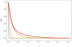
(a) Small Amplitude ($|\epsilon_{in}|=0.1$)

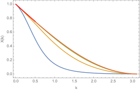
(b) Large Amplitude ($|\epsilon_{in}|=100$)

Figure 12: Momentum mode contribution to the expectation value as a function of the amplitude and the quench rate. Different curves correspond to different quench rates: $J\delta t=100$ is blue; $J\delta t=10$ is yellow; $J\delta t=1$ is green; and $J\delta t=0.1$ overlaps in both figures with the red curve that corresponds to the instantaneous answer (B). The different rate of decay in each figure is clear, showing that only small momenta contribute in the small amplitude case while high modes start contributing for large amplitudes.

In figure 12, we also compare these profiles with the integrand for an ‘instantaneous’ quench, as in Eq. (111). From Eq. (83), this instantaneous integrand takes the simple form

$$X_{inst}(k) = \frac{m(k,t=-\infty)}{\omega(k,t=-\infty)}-\frac{m(k,t=0)}{\omega(k,t=0)}$$

$$= \frac{2\sin^{2}\left(k/2\right)-\epsilon_{in}}{\left[2(2-\epsilon_{in})\sin^{2}\left(k/2\right)+\epsilon_{in}^{2}\right]^{1/2}}-\sin\left(k/2\right)\,,$$

where we have combined the various definitions in section 3 to produce the final expression. Figure 12 shows that for either large or small amplitudes, the integrand $X(k)$ quickly approaches $X_{inst}(k)$ as $J\delta t\to 0$. This will become a key fact in analyzing the modes contribution for small amplitudes, as we will see below. In passing, we also note that with $\epsilon_{in}<0$, $X_{inst}(k=\pi)=0$ and $X_{inst}(k=0)=1$, as was argued must be the case on general grounds above.

Let us first analyze the small amplitude case in more detail. We first determine which modes are contributing significantly to the expectation value. Then since we are interested in understanding when the expectation value saturates, we will ask for which values of $J\delta t$ are all of these modes excited by the quench (as first discussed in section 4.1), and how this varies as we vary the initial amplitude. We approached these questions with a combination of numerical and analytic analyses. In figure 13, we study the decay of the integrand as a function of $|\epsilon_{in}|$. In particular, we find numerically the momentum $k_{max}$ where $X(k)=0.1$, i.e., where the integrand decays to 10 percent of its maximum value. This gives us an estimate of the range of momenta for which the corresponding modes are contributing significantly to the expectation value (123). The result in figure (13) is robust: for any $J\delta t$, there is a region for small enough $|\epsilon_{in}|$ where $k_{max}\propto|\epsilon_{in}|$ and moreover, the coefficient of proportionality is independent of $J\delta t$. However, the coefficient obviously depends on the chosen threshold, i.e., $X(k_{max})=0.1$ in the present case.

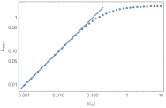
(a) $J\delta t=0.1$

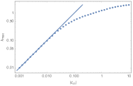
(b) $J\delta t=1$

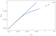
(c) $J\delta t=10$

Figure 13: Numerical evaluation of $k_{max}$ as a function of $|\epsilon_{in}|$ for different values of $J\delta t$. In the three cases, it is possible to observe a linear dependence of $k_{max}$ on $|\epsilon_{in}|$ for small enough $|\epsilon_{in}|$. This is verified by the fit with a function $k_{max}=c\,|\epsilon_{in}|$ (solid blue line). Further, we find the coefficient $c$ is the same in all three plots, i.e., it is independent of $J\delta t$ but depends, of course, on the choice of the threshold, being $X(k_{max})=0.1$ in the present case.

We can also provide an analytic calculation which supports this same conclusion. First, using Eqs. (3) and (75), we can expand the expression in Eq. (124) for $X(k)$ to find

$$X(k)=X_{inst}(k)+O((J\delta t)^{2})\,,$$ (126)

where $X_{inst}$ is given by Eq. (B). Of course, this result is in agreement with the observation that $X(k)$ quickly approaches $X_{inst}(k)$, made from the plots in figure 12. However, this result can be refined since if we carefully examine the expressions in Eqs. (3) and (75), it is possible to see that every contribution of $J\delta t$ to the integrand (124) is accompanied either by a factor of the amplitude $\epsilon_{in}$ or a momentum factor, $\sin(k/2)$. It will serve our purposes below to expand $X(k)$ simultaneously for small $x\equiv\epsilon_{in}\,J\delta t$ and $y\equiv\sin(k/2)\,J\delta t$. With these variables, we find that the previous expansion is replaced by

$$X(k)=X_{inst}(k)+O(y^{2},xy)\,.$$ (127)

where implicitly we have assumed that $x\sim y$ in our expansion. Of course, we may ensure that $|x|,|y|\ll 1$ by simply taking $J\delta t\ll 1$ and with this choice, we recover Eq. (126). However, the above expansion indicates for any $J\delta t\ll 1/|\epsilon_{in}|,1/k$, the integrand is well approximated by the instantaneous integrand. Hence for small amplitudes, as considered here, we may still consider $J\delta t\sim 1$ as long as the relevant momenta are also small. This will now let us self-consistently prove that only small momenta contribute to the expectation value (123) for small amplitude quenches.

Above we argued that in the limit of small momenta and small amplitude, $X(k)$ reduces to the instantaneous integrand. However, it remains to expand the expression in eq. (B) when taking $k,|\epsilon_{in}|\ll 1$ while keeping $k/|\epsilon_{in}|\sim 1$. This expansion yields

$$X_{inst}(k)=-\frac{\epsilon_{in}}{\left[k^{2}+\epsilon_{in}^{2}\right]^{1/2}}-\frac{k}{2}+\frac{(2k^{2}+\epsilon_{in}^{2})k^{2}}{4\left[k^{2}+\epsilon_{in}^{2}\right]^{3/2}}+O(k^{2})\,,$$ (128)

where the $O(k^{2})$ is used above in a sense where the third term is $O(k)$.

Now, to determine the significant contributions, we want to see when the leading term in eq. (128) reaches a particular threshold $\gamma$ in this limit. Hence we set

$$\frac{|\epsilon_{in}|}{\left[k_{max}^{2}+\epsilon_{in}^{2}\right]^{1/2}}=\gamma\quad\implies\quad k_{max}=\frac{\sqrt{1-\gamma^{2}}}{\gamma}\,|\epsilon_{in}|\,,$$ (129)

where we assumed that $\epsilon_{in}<0$ while $\gamma>0$. We note that this $O(1)$ term for $X_{inst}(k)$ in eq. (128) has a long tail. However, let us explicitly evaluate the pre-factor for $\gamma=0.1,\,0.2,\,0.5$, and we find $c\equiv\sqrt{1-\gamma^{2}}/\gamma=9.95,\,4.90,\,1.73$, respectively. So even with $\gamma=0.1$, we have a consistent solution for $k_{max}$. That is, our expansion assumed that the relevant $k$’s were small and now we find that the maximum contributing momentum is proportional to $|\epsilon_{in}|$ and so it is indeed small for the small amplitudes considered here. Moreover, as both the amplitudes and momenta are small, this result is still valid for $J\delta t\sim 1$, which will be needed below for our final result on the saturation point. It is also important that the pre-factor $c$ in eq. (129) is independent of $J\delta t$.

Hence both our numerical and analytic calculations suggest that for small amplitude quenches, the modes which contribute significantly to the expectation value (123) lie in a narrow band: $0\leq k\leq k_{max}$ with $k_{\max}=c\,|\epsilon_{in}|$ where $c$ is some order one number (which is independent of $J\delta t$). Now as discussed in section 4.1, we can expect that the expectation value saturates when all of these modes are in fact excited by the quench. In particular then, we must confirm that the last mode at $k=k_{max}$ is excited according to the Landau criterion (85). Substituting in $k_{\max}=c\,|\epsilon_{in}|$ and keeping in mind that we are considering small amplitude quenches, i.e., $|\epsilon_{in}|\ll 1$, we find

$${\rm small\ amplitude:}\qquad\frac{1}{E_{k_{max}}^{2}}\,\left|\frac{dE_{k_{max}}}{dt}\right|_{t=0}=\frac{1}{4c\,J\delta t}\,,$$ (130)

which should then be larger then one to excite all of the modes contributing to $\langle{\bar{\chi}}\chi\rangle_{\textrm{\tiny diff}}(t=0)$. That is, we expect saturation for $J\delta t\leq 1/(4c)$ or more simply $J\delta t\lesssim 1$. As stressed in the main text, this result shows that for the small amplitude quenches, the point where saturation sets in is independent of the initial amplitude. Note also that while the argument that the maximum momentum contribution is proportional to the initial amplitude is valid for larger $J\delta t$ (provided the amplitude is small enough), the Landau criterion in this case will show that it is still possible to keep exciting these modes and then we will see no saturation for larger $J\delta t$.

The situation is qualitatively different for large amplitude quenches. As shown in figure 12, in this case, the profile of the integrand (124) is much broader and hence almost every mode makes a significant contribution to the expectation value. Hence we essentially have, $k_{max}\simeq\pi$. Of course, the mode $k$ exactly at $\pi$ is not contributing since as noted above, $X(k=\pi)=0$ in every quench, i.e., for any amplitude or quench rate. However, other modes near $\pi$ will contribute significantly to the expectation value. It is straightforward to evaluate the Landau criterion (85) for $k_{max}\simeq\pi$, and as in eq. (86), we obtain

$${\rm large\ amplitude:}\qquad\frac{1}{E_{k_{max}}^{2}}\,\left|\frac{dE_{k_{max}}}{dt}\right|_{t=0}=\frac{|\epsilon_{in}|}{8J\delta t}\,.$$ (131)

As before, all the modes contributing to the expectation value (123) will be excited when the above expression is bigger than one. Hence we should expect saturation for $J\delta t\lesssim|\epsilon_{in}|/8$. This is the result reported in section 4.1, and hence the saturation point is proportional to the initial amplitude for large amplitude quenches. While all of the above analysis is particular to the Transverse Field Ising model, let us re-iterate that we expect an analogous description will hold for the results for the quenches in the Kitaev model described in section 4.2.

Appendix C Cluster-Ising model

The Hamiltonian of the Cluster-Ising model cluster-ising on a one-dimensional bipartite lattice is

$$H_{\textrm{\tiny CI}}=-\sum_{j=1}^{N}\tau^{(1)}(j-1)\tau^{(3)}(j)\tau^{(1)}(j+1)+\lambda(t)\sum_{j=1}^{N}\tau^{(2)}(j)\tau^{(2)}(j+1)\,.$$ (132)

where we have allowed for a time-dependent Ising coupling to consider quenches and $\tau^{(1,2,3)}$ denote Pauli spin operators.

For $\lambda=0$, the ground state is protected by a $\mathbb{Z}_{2}\times\mathbb{Z}_{2}$ symmetry generated by $\prod_{i\in even}\tau_{i}^{z}\times\prod_{i^{\prime}\in odd}\tau_{i^{\prime}}^{z}$. This short-ranged entangled state has topological order (no long range order) on a open chain, realizing projective representations of the symmetry group via edge states. At $\lambda=1$, the model has a quantum critical point and for $\lambda>1$, the system is antiferromagnetic with long range order. At the quantum phase transition, the critical exponents are $\nu=z=1$, $\beta=3/8$ and $\alpha=0$. We show below that on a closed chain with periodic boundary conditions, the model can be mapped to ($1+1$)-dimensional free fermions as in the Ising case.

Introducing Jordan-Wigner fermions,

$$c(j)=\prod_{m=1}^{j-1}\tau^{(3)}(m)\tau^{-}(j).$$

where $\tau_{j}^{\pm}=(\tau^{(1)}(j)\pm i\tau^{(2)}(j))/2$, the Hamiltonian (132) becomes

$$H_{\textrm{\tiny CI}} = \sum_{l=1}^{N}\left(c(l-1)^{\dagger}-c(l-1)^{\vphantom{\dagger}}\right)\left(c^{\dagger}(l+1)+c(l+1)^{\vphantom{\dagger}}\right)$$ (133)

$$+\lambda\sum_{l=1}^{N}\left(c^{\dagger}(l)+c^{\vphantom{\dagger}}(l)\right)\left(c^{\dagger}(l+1)-c^{\vphantom{\dagger}}(l+1)\right)\,.$$

Next we apply the Fourier transform

$$b(k)=\frac{1}{\sqrt{N}}\sum_{j=1}^{N}c(j)\,e^{-ikj}\,.$$ (134)

with

$$k=\pm 2\pi/(2N),\pm 6\pi/(2N)\dots,\pm 2\pi(N-1)/(2N)\,.$$

The spin Hamiltonian (133) can now be written as,

$$H_{\textrm{\tiny CI}}=\sum_{k>0}\chi^{\dagger}(k){\cal H}_{k}\chi^{\vphantom{\dagger}}(k)\,,$$ (135)

where

$${\cal H}_{k}=(\cos 2k-\lambda\cos k)\sigma_{3}+(\sin 2k+\lambda\sin k)\sigma_{2}\,,$$ (136)

$\sigma_{i}$ denotes Pauli matrices in particle-hole space of fermions and $\chi(q)$ is a two-component Majorana fermion defined by

$$\chi(q)=\left(\begin{array}[]{c}b(q)\\ b^{\dagger}(-q)\end{array}\right)\,.$$

To bring this Hamiltionian into a standard Dirac form, we carry out a few unitary transformations. Let us first write the Hamiltonian (136) as

$${\cal H}_{k}=(\alpha_{k}+\beta_{k}\lambda)\,\sigma_{3}+(\gamma_{1k}+\gamma_{2k}\lambda)\,\sigma_{2}\,.$$ (137)

where $\alpha_{k}=\cos 2k$, $\beta_{k}=-\cos k$, $\gamma_{1k}=\sin 2k$ and $\gamma_{2k}=\sin k$. First we do a global rotation by the unitary, $e^{i\sigma_{3}\pi/4}$, which leaves $\sigma_{3}$ invariant and rotates $\sigma_{2}$ into $\sigma_{1}$. Next, let us rewrite the Hamiltonian in terms of new Pauli matrices, $\tau_{i}$ as

$$\tilde{\cal H}_{k}=\Lambda_{1k}(\lambda(t)-t_{1k})\tau_{3}+\Lambda_{2k}\tau_{1}\,.$$ (138)

We have from Eqs. (137) and (138),

$$\Lambda_{1k}\tau_{3} = \beta_{k}\sigma_{3}+\gamma_{2k}\sigma_{1}\,,$$

$$\Lambda_{2k}\tau_{1} = \sigma_{3}(\alpha_{k}+t_{1k}\beta_{k})+\sigma_{1}(\gamma_{1k}+t_{1k}\gamma_{2k})\,.$$

This gives

$$\Lambda_{1k}^{2} = \beta_{k}^{2}+\gamma_{2k}^{2}\,,$$ (139)

$$\Lambda_{2k}^{2} = (\alpha_{k}+t_{1k}\beta_{k})^{2}+(\gamma_{1k}+t_{1k}\gamma_{2k})^{2}\,.$$ (140)

From the canonical condition, $\{\tau_{1},\tau_{3}\}_{+}=0$, we find

$$\beta_{k}(\alpha_{k}+t_{1k}\beta_{k})+\gamma_{2k}(\gamma_{1k}+t_{1k}\gamma_{2k})=0\,.$$ (141)

Using Eqs. (139), (140) and (141), the Hamiltonian can be brought into the form

$$\tilde{\cal H}_{k}=\left(\lambda(t)-\cos 3k\right)\,\tau_{3}+\sin 3k\,\tau_{1}\,.$$ (142)

Note that this expression (142) is the same as the lattice Hamiltonian (20) for the Ising model with the replacement of $k\rightarrow-3k$, and there is a periodicity $k\rightarrow k+\frac{2\pi}{3}$. This means that we can rewrite the theory in terms of three flavors of Majorana fermions, each living on a chain of size $N/3$.

The eigenvalues of the Hamiltonian (142) are

$$E_{k}=\pm\sqrt{1+\lambda(t)^{2}-2\lambda(t)\cos 3k}\,.$$ (143)

Thus we see at $\lambda=1$ the gap closes for $k\rightarrow 0$, $2\pi/3$ and $4\pi/3$. Expanding around this critical point, we can see that the theory is described by three massive Majorana fermions in the continuum limit. With the lattice spacing $a$, we introduce dimensionful momenta $p$, and a dimensionful mass $m$,

$$p=\frac{3k}{a}\qquad{\rm and}\qquad m(t)=\frac{\lambda(t)-1}{a}\,,$$ (144)

the Hamiltonian becomes in the $a\rightarrow 0$ limit

$$H_{\textrm{\tiny CI}}^{\textrm{\tiny cont}}=\sum_{i=1}^{3}\int\frac{dp}{2\pi}\,\psi^{i\dagger}(p)\left[m(t)\,\tau_{3}+p\,\tau_{1}\right]\psi^{i}(p)\,.$$ (145)

which is equivalent to three identical copies of Eq. 27, describing the continuum theory for the Ising model.

References

- (1) T. W. B. Kibble, “Topology of Cosmic Domains and Strings,” J. Phys. A 9, 1387 (1976).
- (2) W. H. Zurek, “Cosmological Experiments in Superfluid Helium?,” Nature 317, 505 (1985).
-
(3)
For example, see the following reviews:
S. Mondal, D. Sen and K. Sengupta, “Non-equilibrium dynamics of quantum systems: order parameter evolution, defect generation, and qubit transfer,” Quantum Quenching, Anealing and Computation, Lecture notes in Physics, 802, 21 (2010) [arXiv:0908.2922[cond-mat.stat-mech]];
V. Gritsev and A. Polkovnikov, “Universal Dynamics Near Quantum Critical Points,” arXiv:0910.3692 [cond-mat.stat-mech].
J. Dziarmaga, “Dynamics of a quantum phase transition and relaxation to a steady state,” Adv. Phys. 59, 1063 (2010) [arXiv:0912.4034 [cond-mat.quant-gas]];
A. Polkovnikov, K. Sengupta, A. Silva and M. Vengalattore, “Nonequilibrium dynamics of closed interacting quantum systems,” Rev. Mod. Phys. 83, 863 (2011) [arXiv:1007.5331 [cond-mat.stat-mech]];
A. Lamacraft and J.E. Moore, “Potential insights into non-equilibrium behaviour from atomic physics,” in Ultracold Bosonic and Fermionic Gases, Contemporary Concepts in Condensed Matter Science, Elsevier (Editors: A. Fletcher, K. Levin and D. Stamper-Kurn) [arXiv:1106.3567[cond-mat.quant-gas]]; -
(4)
A. Chandran, A. Erez, S. S. Gubser and S. L. Sondhi,
“Kibble-Zurek problem: Universality and the scaling limit,”
Phys. Rev. B 86, 064304 (2012) [arXiv:1202.5277 [cond-mat.stat-mech]];
-
(5)
A. Buchel, L. Lehner and R. C. Myers,
“Thermal quenches in N=2* plasmas,”
JHEP 1208, 049 (2012)
[arXiv:1206.6785 [hep-th]];
A. Buchel, L. Lehner, R. C. Myers and A. van Niekerk, “Quantum quenches of holographic plasmas,” JHEP 1305, 067 (2013) [arXiv:1302.2924 [hep-th]]. - (6) A. Buchel, R. C. Myers and A. van Niekerk, “Universality of Abrupt Holographic Quenches,” Phys. Rev. Lett. 111, 201602 (2013) [arXiv:1307.4740 [hep-th]].
-
(7)
S. R. Das, D. A. Galante and R. C. Myers,
“Universal scaling in fast quantum quenches in conformal field theories,”
Phys. Rev. Lett. 112, 171601 (2014)
[arXiv:1401.0560 [hep-th]].
- (8) S. R. Das, D. A. Galante and R. C. Myers, “Universality in fast quantum quenches,” JHEP 1502, 167 (2015) [arXiv:1411.7710 [hep-th]].
- (9) S. R. Das, D. A. Galante and R. C. Myers, “Smooth and fast versus instantaneous quenches in quantum field theory,” JHEP 1508, 073 (2015) doi:10.1007/JHEP08(2015)073 [arXiv:1505.05224 [hep-th]].
- (10) S. R. Das, D. A. Galante and R. C. Myers, “Quantum Quenches in Free Field Theory: Universal Scaling at Any Rate,” JHEP 1605, 164 (2016) doi:10.1007/JHEP05(2016)164 [arXiv:1602.08547 [hep-th]].
- (11) A. Kitaev, “Anyons in an exactly solved model and beyond,” Ann. Phys. (N.Y.) 321, 2 (2006). doi: 10.1016/j.aop.2005.10.005 [arXiv:cond-mat/0506438 [cond-mat.mes-hall]].
-
(12)
J. Dziarmaga, “Dynamics of a Quantum Phase Transition: Exact Solution of the Quantum Ising Model,” Phys. Rev. Lett. 95, 245701 (2005) doi:10.1103/PhysRevLett.95.245701
[arXiv:cond-mat/0509490 [cond-mat.other]];
J. Dziarmaga, “Dynamics of a quantum phase transition in the random Ising model: Logarithmic dependence of the defect density on the transition rate,” Phys. Rev. B 74, 064416 (2006) doi: 10.1103/PhysRevB.74.064416 [arXiv:cond-mat/0603814 [cond-mat.dis-nn]]. -
(13)
K. Sengupta, D. Sen and S. Mondal, “Exact Results for Quench Dynamics and Defect Production in a Two-Dimensional Model,” Phys. Rev. Lett. 100, 077204 (2008)
doi: 10.1103/PhysRevLett.100.077204
[arXiv:0710.1712 [cond-mat.stat-mech]];
S. Mondal, D. Sen and K. Sengupta, “Quench dynamics and defect production in the Kitaev and extended Kitaev models,” Phys. Rev. B 78, 045101 (2008) doi: 10.1103/PhysRevB.78.045101 [arXiv:0802.3986 [cond-mat.stat-mech]]. - (14) T. Hikichi, S. Suzuki, and K. Sengupta, “Slow quench dynamics of the Kitaev model: Anisotropic critical point and effect of disorder,” Phys. Rev. B 82, 174305 (2010) doi: 10.1103/PhysRevB.82.174305 [arXiv:1009.0323 [cond-mat.str-el]].
- (15) K. Sengupta, S. Powell and S. Sachdev, “Quench dynamics across quantum critical points,” Phys. Rev. A 69, 053616 (2004) doi: 10.1103/PhysRevA.69.053616 [arXiv:cond-mat/0311355 [cond-mat.str-el]].
-
(16)
P. Calabrese and J. L. Cardy,
“Time-dependence of correlation functions following a quantum quench,”
Phys. Rev. Lett. 96, 136801 (2006)
[cond-mat/0601225];
P. Calabrese and J. Cardy, “Quantum Quenches in Extended Systems,” [arXiv:0704.1880 [cond-mat.stat-mech]]. - (17) A. A. Patel, A. Dutta, “Sudden quenching in the Kitaev honeycomb model: Study of defect and heat generation,” Phys. Rev. B 86, 174306 (2012) [arXiv:1209.0072 [cond-mat.stat-mech]].
- (18) M. Schmitt, S. Kehrein, “Dynamical Quantum Phase Transitions in the Kitaev Honeycomb Model ,” Phys. Rev. B 92, 075114 (2015) [arXiv:1505.03401 [cond-mat.stat-mech]].
- (19) S. Sotiriadis and J. Cardy, “Quantum quench in interacting field theory: A Self-consistent approximation,” Phys. Rev. B 81, 134305 (2010) [arXiv:1002.0167 [quant-ph]].
-
(20)
G. Mandal, R. Sinha and N. Sorokhaibam,
“Thermalization with chemical potentials, and higher spin black holes,”
JHEP 1508, 013 (2015)
doi:10.1007/JHEP08(2015)013
[arXiv:1501.04580 [hep-th]];
G. Mandal, S. Paranjape and N. Sorokhaibam, “Thermalization in 2D critical quench and UV/IR mixing,” arXiv:1512.02187 [hep-th]. - (21) J. S. Cotler, M. P. Hertzberg, M. Mezei and M. T. Mueller, JHEP 1611, 166 (2016) doi:10.1007/JHEP11(2016)166 [arXiv:1609.00872 [hep-th]].
- (22) J. B. Kogut, “An Introduction to Lattice Gauge Theory and Spin Systems,” Rev. Mod. Phys. 51, 659 (1979). doi:10.1103/RevModPhys.51.659
- (23) P. Smacchia, L. Amico, P. Facchi, R. Fazio, G. Florio, S. Pascazio and V. Vedral, “Statistical mechanics of the cluster Ising model,” Phys. Rev. A, 84, 2, (2011) doi:10.1103/PhysRevA.84.022304 [arXiv:1105.0853 [quant-ph]].
- (24) H. D. Chen and Z. Nussinov, “Exact results on the Kitaev model on a hexagonal lattice: spin states, string and brane correlators, and anyonic excitations,” [arXiv:cond-mat/0703633]; Z. Nussinov and G. Ortiz, “Autocorrelations and thermal fragility of anyonic loops in topologically quantum ordered systems,” Phys. Rev. B 77, 064302 (2008) doi: 10.1103/PhysRevB.77.064302 [arXiv:0709.2717 [cond-mat.str-el]].
- (25) X.-Y. Feng, G.-M. Zhang, and T. Xiang, “Topological Characterization of Quantum Phase Transitions in a Spin-1/2 Model,” Phys. Rev. Lett. 98, 087204 (2007) doi: 10.1103/PhysRevLett.98.087204 [arXiv:cond-mat/0610626 [cond-mat.str-el]].
- (26) A. Duncan, “Explicit Dimensional Renormalization of Quantum Field Theory in Curved Space-Time,” Phys. Rev. D 17, 964 (1978).
- (27) E. Barouch and B. McCoy, “Statistical Mechanics of the XY Model. I,” Phys. Rev. A 2, 1075 (1970).
- (28) T. Hartman, S. Jain and S. Kundu, “Causality Constraints in Conformal Field Theory,” JHEP 1605, 099 (2016) doi:10.1007/JHEP05(2016)099 [arXiv:1509.00014 [hep-th]].