PNe and H II regions in the starburst irregular galaxy NGC 4449 from LBT MODS data

Abstract

We present deep 3500$-$10000 Å spectra of H II regions and planetary nebulae (PNe) in the starburst irregular galaxy NGC 4449, acquired with the Multi Object Double Spectrograph at the Large Binocular Telescope. Using the “direct” method, we derived the abundance of He, N, O, Ne, Ar, and S in six H II regions and in four PNe in NGC 4449. This is the first case of PNe studied in a starburst irregular outside the Local Group. Our H II region and PN sample extends over a galacto-centric distance range of $\approx$2 kpc and spans $\approx$0.2 dex in oxygen abundance, with average values of $12+\log(O/H)=8.37\pm 0.05$ and $8.3\pm 0.1$ for H II regions and PNe, respectively. PNe and H II regions exhibit similar oxygen abundances in the galacto-centric distance range of overlap, while PNe appear more than $\sim$1 dex enhanced in nitrogen with respect to H II regions. The latter result is the natural consequence of N being mostly synthesized in intermediate-mass stars and brought to the stellar surface during dredge-up episodes. On the other hand, the similarity in O abundance between H II regions and PNe suggests that NGC 4449’ s interstellar medium has been poorly enriched in $\alpha$-elements since the progenitors of the PNe were formed. Finally, our data reveal the presence of a negative oxygen gradient for both H II regions and PNe, whilst nitrogen does not exhibit any significant radial trend. We ascribe the (unexpected) nitrogen behaviour as due to local N enrichment by the conspicuous Wolf-Rayet population in NGC 4449.

1. Introduction

Stellar and galaxy evolution are closely coupled: on the one hand, subsequent generations of high- and intermediate-mass stars continuously modify the energy balance and chemical composition of the interstellar medium (ISM) of their host galaxy; on the other hand gas accretion by diffuse or filamentary cold streams (Dekel et al., 2009) or by gas-rich dwarfs may trigger new star formation and dilute the metallicity of the ISM. It is thus mandatory to combine accurate star formation histories (SFHs) from resolved stellar studies and chemical abundance studies in individual systems as key ingredients to reconstruct a coherent and complete picture of how galaxies formed and evolved.

Since the advent of the Hubble Space Telescope (HST), much effort has been done to resolve the individual stars and to derive the SFHs in large galaxy samples within the Local Universe (e.g., Dalcanton et al., 2009; McQuinn et al., 2010; Monelli et al., 2010a, b; Weisz et al., 2011; Dalcanton et al., 2012; Weisz et al., 2014; Calzetti et al., 2015, see also Tolstoy, Hill & Tosi (2009) for a review). At the same time, the availability of multi-object spectroscopy on 8-10 m telescopes has promoted chemical composition studies of H II regions and planetary nebulae (PNe) over large galaxy areas (e.g., Bresolin et al., 2005; Magrini et al., 2005; Peña et al., 2007; Bresolin et al., 2009b; Magrini & Gonçalves, 2009; Stasińska et al., 2013; Annibali et al., 2015; Berg et al., 2015). In particular, the simultaneous study of chemical abundances in PNe and in H II regions can provide more stringent constraints on chemical evolution models, since H II regions probe the present-day composition of the ISM, while PNe, being the end-product of the evolution of stars with masses 0.8$M_{\odot}$$<$ M $<$ 8 $M_{\odot}$, offer a view of the ISM composition back to several Gyrs ago.

PNe enrich the ISM mainly in He, C and N, while leaving untouched elements such as Ne, S and Ar whose abundance remains the initial one of the PN progenitor. O is also usually thought to be unaffected by the progenitor reaction processes, although it has sometimes been suggested to be enhanced (Marigo, 2001) in metal-poor PNe. The important production of He, C and N by PNe is due to dredge-up episodes occurring during the red giant branch (RGB) and asymptotic giant branch (AGB) phases of intermediate- and low-mass stars, and to hot-bottom burning (HBB, e.g. Renzini & Voli, 1981) in the most massive AGB stars ($\;\lower 2.58334pt\hbox{$\sim$}\kern-7.75pt\raise 2.79857pt\hbox{$>$}\;4M_{\odot}$, depending on metallicity), that change the stellar surface abundances of these elements.

Here we exploited the high performance of the Multi Object Double Spectrograph (MODS) mounted on the Large Binocular Telescope (LBT) to perform the first combined study of H II regions and PNe in the irregular galaxy NGC 4449 ($\alpha_{2000}=12^{h}~{}28^{m}~{}11^{s}.9$, $\delta_{2000}=+44^{\circ}~{}05^{\prime}~{}40^{\prime\prime}$), at a distance of 3.82$\pm$0.27 Mpc from us (Annibali et al., 2008). NGC 4449 is of particular interest because it is one of the strongest starburst in the local Universe (star formation rate$\sim$1 M_⊙ yr^-1, or $\sim$0.04 M_⊙ yr^-1 kpc^-2, McQuinn et al., 2010; Annibali et al., 2011), and moreover it exhibits several characteristics suggesting that it has accreted one or possibly several smaller companions: more specifically, i) it has a very extended H I halo ($\approx$90 kpc in diameter), which is a factor of $\sim$10 larger than the optical diameter of the galaxy and rotates in the opposite direction to the gas in the center (Hunter et al., 1998); ii) it is one of the very few dwarf galaxies where a stellar tidal stream has been discovered so far (Martínez-Delgado et al., 2012; Rich et al., 2012); iii) it hosts an old, $10^{6}$ $M_{\odot}$cluster associated with two tails of young stars, potentially the nucleus of an accreted gas-rich satellite galaxy (Annibali et al., 2012). Because of these properties, NGC 4449 is a perfect laboratory to test the hypothesis that strong starbursts in dwarf galaxies are caused by accretion or merging events, as suggested by recent studies showing that disturbed H I kinematics, H I companions, and filamentary H I structures are more common in starburst dwarfs than in typical star-forming irregulars (Lelli et al., 2014). NGC 4449 was targeted with the Advanced Camera for Survey (ACS) on board of HST a few years ago to resolve its stellar content and to derive its SFH (Annibali et al., 2008; McQuinn et al., 2010; Sacchi et al., 2017). These analyses indicate that NGC 4449 enhanced its SF activity $\approx$500 Myr ago, while the rate was much lower at earlier epochs; however, the impossibility to reach, even with HST, the main sequence turnoffs at a distance of $\sim$4 Mpc implies that the SFH of NGC 4449 is very uncertain prior to $1-2$ Gyr ago (see e.g. Sacchi et al., 2017).

In this paper we present a study of the H II region and PN chemical abundances in NGC 4449 with the purpose of providing a key complement to previous stellar population studies. Chemical evolution models based on the SFH and on the derived abundances (see e.g. the approach of Romano et al., 2006) will be presented in a forthcoming paper and will provide new insights into the past evolution of NGC 4449. The paper is structured as follows: Section 2 describes the observations and data reduction, Section 3 informs on the procedure for the derivation of the reddening-corrected emission line fluxes, while temperatures, densities, and chemical abundances of H II regions and PNe are derived in Section 4. Section 5 focuses on the study of the Wolf-Rayet spectral features. In Section 6 and 7 we analyse and discuss the derived abundances, element ratios and spatial abundance distributions, while in Section 8 we compare the properties of our PNe with those of Local Group star forming dwarfs. Our conclusions are summarised in Section 9.

2. Observations and data reduction

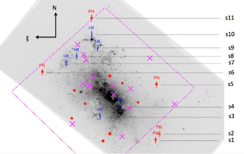
Figure 1.— HST/ACS image of NGC 4449 in F555W ($\sim$V) with superimposed our H II region and PN sample. The smaller field of view covered by the ACS F502N ($\sim$[O III]) image is also indicated with the magenta line. The small red points and magenta crosses indicate the totality of the 28 PNe identified from the combined F435W ($\sim$B)-F502N - F814W (I) image, and then cross-checked in F658N (H$\alpha$). The small red points denote the 13 PNe also identified when using the combined B, V, I image. Superimposed on the image are the eleven LBT/MODS 1”$\times$10” slits at the position of the 6 H II regions and 5 PNe targeted for spectroscopy.

PN candidates and H II regions were identified on HST/ACS images in the F435W ($\sim$ B), F555W ($\sim$ V), F814W ($\sim$ I), and F658N (H$\alpha$) filters (GO program 10585; PI: Aloisi). These data cover a field of view as large as $\sim 400^{\prime\prime}\times 200$” (two ACS pointings) and allow to identify both H II regions and PNe up to large galacto-centric distances. In the ACS images, H II regions are resolved and appear as regions of diffuse H$\alpha$ and V (i.e. [OIII]$\lambda\lambda$4959,5007) emission. On the other hand, PN candidates were visually selected from a B, V, I color-combined image looking for point-like sources that stand out in V compared to B and I because of the [OIII]$\lambda\lambda$4959,5007 emission lines. The 29 selected candidates were then cross-identified on the shallower H$\alpha$ image to eliminate background emission-line sources. This provided 13 PN candidates in NGC 4449, whose spatial location is shown in Figure 1. We repeated the PN search using archival ACS images in the narrow-band F502N filter (GO program 10522, PI Calzetti) instead of the F555W image and then cross-checked in H$\alpha$. The F502N filter, centered around the [O III]$\lambda$5007 line, allows for a better contrast of the PNe compared to stars; however, the smaller $\sim 200^{\prime\prime}\times 200$” field of view of the available data (corresponding to just one ACS pointing) does not permit an inspection of the NGC 4449 outskirts where PNe can be more easily studied thanks to the lower galaxy background. All the PNe that were identified from the F555W image were also found when using the F502N image (however three PNe fall outside the field of view of the F502N image); 15 additional PNe were identified when adopting the F502N image in place of the F555W one (see Figure 1), for a total sample of 28 PNe.

PNe and H II regions were targeted for spectroscopy with LBT/MODS from January 21, 2013 until April 5, 2013 within program 2012B_23, RUN A (PI Annibali). The 1”$\times$10” slit mask is shown in Figure 1. We were able to accomodate into the MODS slit mask 5 PNe out of 28, chosen in the most external regions of NGC 4449 to minimize the contamination from the diffuse ionized gas. Six remaining slits were positioned on H II regions. Figure 2 shows color-composite HST images for the PNe and H II regions targeted with LBT, with superimposed the MODS slits. We observed our targets using the blue G400L (3200$-$5800 Å) and the red G670L (5000$-$10000 Å) gratings on the blue and red channels in dichroic mode for a total exposure time of $\sim$10.5 h, organized into 14 sub-exposures of $\sim$2700 s each. The seeing varied between $\sim$0.6” and $\sim$1.3”, and the airmass from $\sim$1.0 to $\sim$1.3. Typically, the exposures were acquired at hour angles between $\sim$ $-$1 h and $\sim$ $+$1 h to avoid significant effects from differential atmospheric refraction (see e.g. Filippenko, 1982). Only 8 sub-exposures with a seeing $\lesssim 1^{\prime\prime}$ were retained for our study, for a total integration time of $\sim$ 6 h. The journal of the observations is provided in Table 1.

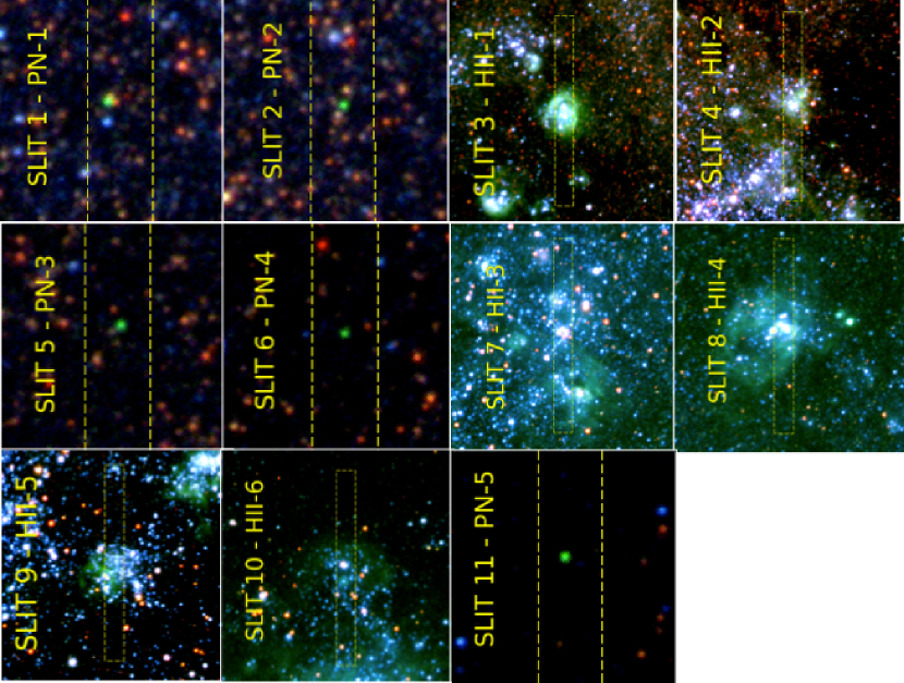
Figure 2.— HST/ACS color-combined images (F435W$=$blue, F555W$=$green, F814W$=$red) of PNe and H II regions in NGC 4449 targeted for spectroscopy with LBT/MODS. The FoV shown is $\sim 3.5^{\prime\prime}\times 3.5^{\prime\prime}$ for the PNe and $12^{\prime\prime}\times 12^{\prime\prime}$ for the H II regions.

Table 1Journal of LBT/MODS observations

Exp.N.	Date-obs	Exptime	Seeing	Airmass	Retained?
1	2013-01-21	2700 s	0.6”	1.0	yes
2	2013-01-21	2700 s	0.6”	1.0	yes
3	2013-01-21	2700 s	0.7”	1.0	yes
4	2013-04-01	2700 s	1.0”	1.1	yes
5	2013-04-01	2700 s	0.8”	1.1	yes
6	2013-04-01	2700 s	0.7”	1.0	yes
7	2013-04-01	2700 s	0.8”	1.0	yes
8	2013-04-01	2700 s	1.1”	1.0	no
9	2013-04-01	2700 s	1.1”	1.1	no
10	2013-04-01	2700 s	1.1”	1.2	no
11	2013-04-01	3040 s	2.0”	1.3	no
12	2013-04-02	2700 s	0.9”	1.0	yes
13	2013-04-02	2700 s	1.3”	1.1	no
14	2013-04-05	2700 s	1.3”	1.0	no

Bias, flat-field, and wavelength calibrations were performed with the Italian LBT Spectroscopic reduction Facility at INAF-IASF Milano, producing the calibrated two-dimensional (2D) spectra for the individual sub-exposures. Then, the individual sub-exposures were sky-subtracted and combined into final 2D blue and red frames. The sky subtraction was performed with the background task in IRAF, typically choosing the windows at the two opposite sides of the central source. This procedure removed, together with the sky, also the contribution from the NGC 4449 unresolved background. As an example, we show in Figure 3 the two-dimensional sky-subtracted combined spectra for our PNe in selected spectral regions. The figure shows that we were able to detect the [O III]$\lambda$4363 line in all PNe thanks both to the good MODS resolution and to the NGC 4449’ s systemic velocity of $\approx$210 km s^-1, allowing for sufficient separation with the Hg I $\lambda$4358 sky line. For region H II-3, located in slit 7, it was not possible to evaluate the background, since the slit was entirely filled by gaseous emission. In this case, we adopted the background derived for PN 5 (slit 11) as a sky template, and subtracted it to region H II-3. This is a reasonable choice because PN 5 is located at fairly large galactocentric distance and is affected by negligible contribution from the NGC 4449 unresolved background. The one-dimensional (1D) spectra were extracted from the 2D calibrated and sky-subtracted spectra by running the apall task in the twodspec IRAF package. To derive the effective spectral resolution, we used the combined 1D spectra with no sky subtraction, and measured the FWHM of the most prominent sky lines; this resulted into FWHM$\approx$4.1 Å (or R$\sim$1100 at 4500 Å) for the blue channel, and FWHM$\approx$5.8 Å (or R$\sim$1400 at 8000 Å) for the red channel.

The blue and red 1D spectra were flux calibrated using the sensitivity curves from the Italian LBT spectroscopic reduction pipeline; the curves were derived using the spectrophotometric standard star Feige 56 observed in dichroic mode with a 5”-width slit on April 1, 2013 at an airmass of $\sim$1.4. To obtain the red and blue sensitivity curves, the observed standard was compared with reference spectra in the HST CALSPEC database. Atmospheric extinction corrections were applied using the average extinction curve available from the MODS calibration webpage at http://www.astronomy.ohio-state.edu/MODS/Calib/. This may introduce some uncertainty in flux calibration, in particular at the bluest wavelengths, where the effect of atmospheric extinction is more severe. By comparing the sensitivity curves from Feige 56 with those obtained from another standard, Feige 66, observed on January 20, 2013 at an airmass of $\sim$1 and with the same setup of Feige 56 as part of our 2012B_23, RUN B program, we found a $\sim 15\%$ difference at wavelegnths below $\sim$ 4000 Å, while the curves agree within $\sim 1\%$ at redder wavelengths.

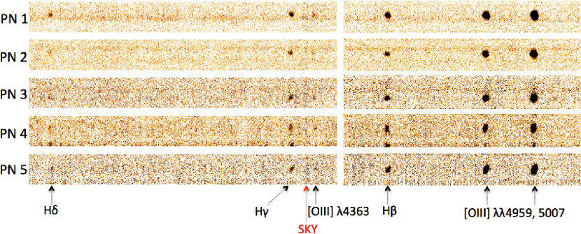
Figure 3.— Two-dimensional MODS spectra of PNe in NGC 4449 showing the H$\delta$, H$\gamma$, [O III]$\lambda$4363, H$\beta$ and [O III]$\lambda\lambda$4959, 5007 lines. The residuals corresponding to the subtraction of the Hg I $\lambda$4358 sky line, between the H$\gamma$ and [O III]$\lambda$4363 lines, are visible in the 2D spectra.

Figure 4.— Comparison between ACS and Synphot fluxes for H II regions in NGC 4449 (see Section 2). From blue to red wavelengths, the dots correspond to the following ACS bandpasses: F435W, F502N, F555W, F550M, F658N and F814W. For each H II region, the solid horizontal line is the average $log(F_{\lambda,ACS})-log(F_{\lambda,SYN})$ offset. The standard deviation around this value is also indicated within each panel.

Figure 5.— LBT/MODS spectra in the blue and red channels for H II-1 in NGC 4449 with indicated all the identified emission lines. A linear interpolation was performed in the 5400 - 5800 Å region where the sensitivities of the blue and red detectors drop. The spectra of the other H II regions (H II-2, H II-3, H II-4, H II-5, H II-6) are provided in the Appendix.

Figure 6.— LBT/MODS spectra in the blue and red channels for PN-1 in NGC 4449 with indicated all the identified emission lines. A linear interpolation was performed in the 5400 - 5800 Å region where the sensitivities of the blue and red detectors drop. A $\sim$1 Å boxcar filter smoothing was applied to the spectrum to better highlight the low singal-to-noise features. The spectra of the other PNe (PN-2, PN-3, PN-4, PN-5) are provided in the Appendix.

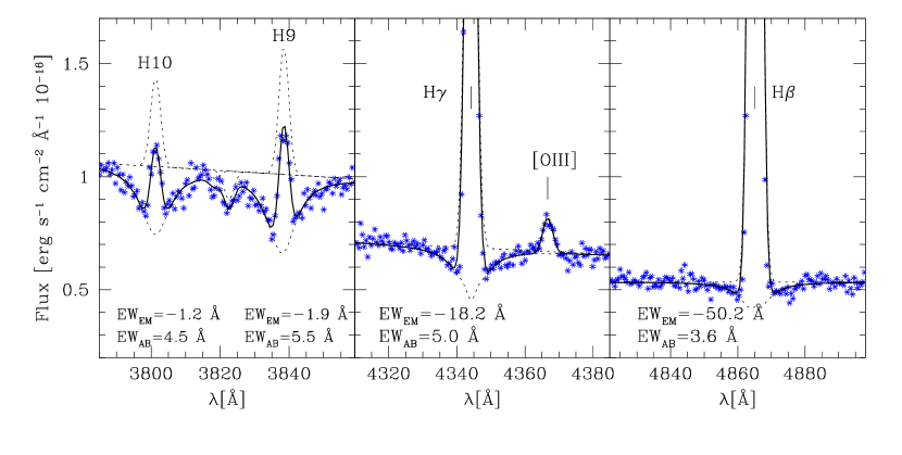
Figure 7.— Example (region H II-6) of spectral fit to the regions around some Balmer lines. The asterisks are the observed spectrum, while the continuous line is the best fit. The individual components of the fit are plotted with a dashed line: linear continuum, Gaussian profiles for the emission lines, and Voigt profiles for the Balmer absorption lines. The outcome of fit to the H10($\lambda$3798) and H9($\lambda$3835) lines, with prominent absorption wings, was used to fix the Lorentian and Gaussian FWHMs during the fit to redder Balmer lines. The derived Balmer equivalent widths in absorption and in emission are provided within each panel. The absorption feature between H10 and H9 is due to a blend of Fe I lines. The figure clearly shows that the contribution of absorption with respect to emission becomes increasingly lower toward redder wavelengths (see section 3.1 for more details.)

Eventually, to evaluate the accuracy of the flux calibration for our spectra, we used HST/ACS imaging in F435W, F555W, F814W, and F658N from our GO program 10585 and archive HST/ACS imaging in F502N and F550M from GO program 10522 (PI Calzetti), with a smaller field of view. The six H II regions, plus PN-3 and PN-4, fall within the field of view of all six images; however, we considered only H II regions to the purpose of checking the flux calibration, because of their signal-to-noise higher than in PNe. Aperture photometry was performed on the images within the same extraction aperture of the 1D spetcra using the Polyphot task in IRAF. The F555W magnitudes in the ACS Vegamag system derived for the H II regions and the 5 PNe targeted with MODS are given in Tables 2 and 3 in the Appendix (see instead Table 9 in Section 8 for a complete list of the F555W and the F502N magnitudes derived for the total sample of 28 PNe). For the H II regions, we also computed synthetic magnitudes in the F435W, F502N, F550M, F555W, F814W and F658N ACS filters by convolving the MODS spectra with the ACS bandpasses: this was done by running the Calcphot task in the Synphot package. Figure 4 shows, for each H II region, the comparison between the observed ACS fluxes and the synthetic ones (in logarithmic scale) as a function of wavelength. We notice that the $F_{\lambda,ACS}$ fluxes are smaller than the $F_{\lambda,SYN}$ ones, indicating that the fluxes from the spectra are overestimated. This effect is expected, and its origin is well discussed by Smith et al. (2007): flux calibrations are usually tied to reference point source observations, and therefore include an implicit correction for the fraction of the point source light that falls outside the slit; however, in the limit of a perfect uniform, slit-filling extended source, the diffractive losses out of the slit are perfectly balanced by the diffractive gains into the slit from emission beyond its geometric boundary. Therefore, the point-source-based calibration will inevitably cause an overestimate of the extended source flux. The $\log(F_{\lambda,ACS})-\log(F_{\lambda,SYN})$ zero point offsets of Fig. 4 were used to anchor our H II region spectra to the ACS magnitudes; this procedure is useful to establish an absolute flux calibration for these objects. On the other hand, no correction was applied to the PN spectra, for two main reasons: 1) these sources are point-like at NGC 4449’ s distance (also in the HST images), and therefore we do not expect the spectral fluxes to be overestimated as in the case of extended H II regions; 2) synthetic fluxes derived by convolving the ACS filter throughputs with the PN spectra are highly affected by uncertainties in the background subtraction, and do not permit a reliable comparison with the ACS photometry. The standard deviation around the average $\log F_{\lambda,ACS}-logF_{\lambda,SYN}$ value derived for the H II regions is quite modest, corresponding to an average flux uncertainty in the range $\approx$2% - $\approx$11%. The low dispersion about the mean and the lack of a general trend with wavelength apparently confirms that our observational setup prevented significant flux losses at the bluest wavelengths due to atmospheric differential refraction (Filippenko, 1982).

As an example, we show the final calibrated spectra for H II region H II-1 and planetary nebula PN-1 in Figures 5 and  6, respectively. The spectra of all the other H II regions and PNe are provided in Figures 16 to  24 in the Appendix.

3. Emission line measurement

Emission line fluxes for H II regions and PNe were obtained with the deblend function available in the splot IRAF task. We used this function to fit single lines, groups of lines close in wavelength, or blended lines. Lines were fitted with Gaussian profiles, treating the centroids and the widths as free parameters; however, when fitting groups of lines close in $\lambda$ (e.g., ${\rm He~{}I~{}\lambda 6678+[S~{}II]\lambda 6716+[S~{}II]\lambda 6731}$) or (partially) blended (${\rm H\alpha+[N~{}II]\lambda\lambda 6548,84}$), we forced the lines to have all the same width. On the other hand, no constraint on the line centroids (e.g. fixed separation between the lines) was assumed and we let the deblend function to find the best-fit line centers independently. This was a reasonable choice given that even faint “key” lines, such as [O III]$\lambda 4363$ and [N II]$\lambda\lambda 6548,84$, are detected with a good signal-to-noise in our spectra; however, had we had worse data, it would have been more appropriate to set the wavelengths of the blended lines and to allow for a common Doppler shift, in order to reduce the noise on the weak lines measurement. The continuum was defined choosing two continuum windows to the left and to the right of the line or line complex, and fitting with a linear regression. Balmer lines, potentially affected by underlying stellar absorption, were fitted with a combination of Voigt profiles in absorption plus Gaussian profiles in emission (see Section 3.1 for more details).

The final emission fluxes were obtained repeating the measurement several times with slightly different continuum choices, and averaging the results. To compute the errors, we derived the standard deviation of the different measurements ($\sigma_{F,line}$). The results for the H II regions and the PNe are provided in Tables 2 and  3 of the Appendix, respectively. From the tables, we notice that the errors on the derived fluxes are very small: for instance, in the case of H II regions, $\sigma_{F,line}$ is below 1% for the brightest lines such as [O III]$\lambda 5007$. To get more realistic errors, we added in quadrature to $\sigma_{F,line}$ a 15% flux error below $\sim 4000$ Å to account for atmospheric extinction uncertainties (see Section 2), and a 2% to 11% flux error, corresponding to the scatter around the average offsets in Figure 4, at redder wavelengths. For PNe, the standard deviation from the different line measurements turned out significantly larger than for H II regions, typically in the range $\approx$2% to $\approx$20%; an arbitrary additional 15% error, equalling the flux calibration uncertainty below $\sim 4000$ Å  and slightly above the largest scatter for the H II regions in Fig. 4, was added in quadrature to $\sigma_{F,line}$ over the entire wavelength range.

3.1. Absorption from underlying stellar population

Table 4Reddening-corrected emission fluxes for H II regions in NGC 4449

Line	H II-1	H II-2	H II-3	H II-4	H II-5	H II-6
[O II] $\lambda$3727	110 $\pm$ 20	190 $\pm$ 30	400 $\pm$ 70	250 $\pm$ 50	240 $\pm$ 40	480 $\pm$ 90
H10 $\lambda$3978	6 $\pm$ 1	6 $\pm$ 1	6 $\pm$ 1	7 $\pm$ 1	6 $\pm$ 1	6 $\pm$ 1
He I $\lambda$3820	0.9 $\pm$ 0.1	0.7 $\pm$ 0.1	$-$	0.6 $\pm$ 0.1	$-$	$-$
H9$+$He II $\lambda$3835	9 $\pm$ 1	8 $\pm$ 1	9 $\pm$ 1	9 $\pm$ 2	8 $\pm$ 1	9 $\pm$ 2
[Ne III] $\lambda$3869	32 $\pm$ 5	23 $\pm$ 4	14 $\pm$ 2	23 $\pm$ 4	18 $\pm$ 3	35 $\pm$ 6
H8$+$He I $\lambda$3889	19 $\pm$ 3	21 $\pm$ 4	20 $\pm$ 3	22 $\pm$ 4	21 $\pm$ 4	21 $\pm$ 4
H$\epsilon$ $+$ He I $+$[Ne III] $\lambda$3970	25 $\pm$ 4	23 $\pm$ 4	21 $\pm$ 3	27 $\pm$ 5	24 $\pm$ 4	29 $\pm$ 5
He I $\lambda$4026	2.02 $\pm$ 0.06	1.8 $\pm$ 0.2	0.9 $\pm$ 0.1	1.5 $\pm$ 0.2	1.0 $\pm$ 0.1	$-$
[S II] $\lambda$4068	0.73 $\pm$ 0.03	0.77 $\pm$ 0.07	2.5 $\pm$ 0.2	1.0 $\pm$ 0.1	1.3 $\pm$ 0.2	3.9 $\pm$ 0.5
[S II] $\lambda$4076	0.21 $\pm$ 0.03	0.40 $\pm$ 0.04	0.79 $\pm$ 0.06	$-$	$-$	1.5 $\pm$ 0.2
H$\delta$ $\lambda$4101	26.3 $\pm$ 0.8	29 $\pm$ 3	30 $\pm$ 2	33 $\pm$ 5	30 $\pm$ 4	30 $\pm$ 4
H$\gamma$ $\lambda$4340	46 $\pm$ 1	49 $\pm$ 4	50 $\pm$ 4	50 $\pm$ 7	50 $\pm$ 6	52 $\pm$ 6
[O III] $\lambda$4363	2.1 $\pm$ 0.1	1.8 $\pm$ 0.2	1.4 $\pm$ 0.1	1.6 $\pm$ 0.2	1.9 $\pm$ 0.2	2.4 $\pm$ 0.3
He I $\lambda$4389	0.57 $\pm$ 0.02	0.38 $\pm$ 0.03	$-$	0.48 $\pm$ 0.07	$-$	$-$
He I $\lambda$4471	4.6 $\pm$ 0.1	4.8 $\pm$ 0.4	4.1 $\pm$ 0.3	4.5 $\pm$ 0.6	4.2 $\pm$ 0.4	4.2 $\pm$ 0.4
[N III](WR) $\lambda$4640	0.19 $\pm$ 0.01	$-$	$-$	1.1 $\pm$ 0.2	$-$	$-$
[C III](WR) $\lambda$4652	0.11 $\pm$ 0.03	$-$	$-$	0.5 $\pm$ 0.1	$-$	$-$
[Fe III] $\lambda$4658	0.14 $\pm$ 0.02	0.28 $\pm$ 0.02	0.84 $\pm$ 0.06	0.43 $\pm$ 0.07	0.50 $\pm$ 0.06	1.4 $\pm$ 0.2
He II (WR) $\lambda$4686	3.6 $\pm$ 0.2	$-$	$-$	6 $\pm$ 1	$-$	$-$
He II $\lambda$4686	0.4 $\pm$ 0.3	$-$	$-$	$-$	$-$	0.8 $\pm$ 0.1
[Ar IV]$+$He I $\lambda$4713	0.50 $\pm$ 0.05	0.38 $\pm$ 0.03	$-$	0.5 $\pm$ 0.1	$-$	$-$
[Ar IV] $\lambda$4740	0.16 $\pm$ 0.01	$-$	$-$	0.30 $\pm$ 0.06	$-$	$-$
H$\beta$ $\lambda$4861	100 $\pm$ 3	100 $\pm$ 8	100 $\pm$ 7	100 $\pm$ 14	100 $\pm$ 11	100 $\pm$ 11
He I $\lambda$4922	1.20 $\pm$ 0.04	1.2 $\pm$ 0.1	0.76 $\pm$ 0.06	1.0 $\pm$ 0.2	0.8 $\pm$ 0.1	$-$
[O III] $\lambda$4959	143 $\pm$ 4	129 $\pm$ 11	71 $\pm$ 5	100 $\pm$ 20	110 $\pm$ 10	100 $\pm$ 10
[Fe III] $\lambda$4986	0.19 $\pm$ 0.02	0.37 $\pm$ 0.06	1.16 $\pm$ 0.09	0.38 $\pm$ 0.05	0.57 $\pm$ 0.07	1.9 $\pm$ 0.2
[O III] $\lambda$5007	420 $\pm$ 10	380 $\pm$ 30	210 $\pm$ 10	300 $\pm$ 40	320 $\pm$ 40	300 $\pm$ 30
He I $\lambda$5015	2.46 $\pm$ 0.07	2.7 $\pm$ 0.2	2.2 $\pm$ 0.2	2.3 $\pm$ 0.3	2.2 $\pm$ 0.2	2.2 $\pm$ 0.3
[N I] $\lambda$5199	0.21 $\pm$ 0.01	0.13 $\pm$ 0.01	1.01 $\pm$ 0.08	0.26 $\pm$ 0.04	0.34 $\pm$ 0.04	2.2 $\pm$ 0.2
He I $\lambda$5876	11.8 $\pm$ 0.3	12 $\pm$ 1	10.8 $\pm$ 0.8	12 $\pm$ 2	12 $\pm$ 1	13 $\pm$ 1
[OI] $\lambda$6302	1.17 $\pm$ 0.04	0.64 $\pm$ 0.06	$-$	1.1 $\pm$ 0.2	1.7 $\pm$ 0.2	9.4 $\pm$ 1.1
[S III] $\lambda$6314	1.12 $\pm$ 0.03	1.3 $\pm$ 0.1	1.2 $\pm$ 0.1	1.2 $\pm$ 0.2	1.3 $\pm$ 0.2	1.6 $\pm$ 0.2
[OI] $\lambda$6365	0.37 $\pm$ 0.01	0.17 $\pm$ 0.02	2.0 $\pm$ 0.2	0.39 $\pm$ 0.06	0.61 $\pm$ 0.08	3.1 $\pm$ 0.4
[NII] $\lambda$6548	2.9 $\pm$ 0.1	4.2 $\pm$ 0.4	8.8 $\pm$ 0.9	5.3 $\pm$ 0.8	4.9 $\pm$ 0.6	12 $\pm$ 1
H$\alpha$ $\lambda$6563	287 $\pm$ 8	300 $\pm$ 30	300 $\pm$ 30	310 $\pm$ 50	300 $\pm$ 40	310 $\pm$ 40
[N II] $\lambda$6584	8.0 $\pm$ 0.3	12 $\pm$ 1	25 $\pm$ 2	16 $\pm$ 2	14 $\pm$ 2	35 $\pm$ 4
He I $\lambda$6678	3.5 $\pm$ 0.1	3.4 $\pm$ 0.3	3.4 $\pm$ 0.3	3.7 $\pm$ 0.6	3.4 $\pm$ 0.4	3.8 $\pm$ 0.5
[S II] $\lambda$6716	8.2 $\pm$ 0.2	7.1 $\pm$ 0.7	33 $\pm$ 3	15 $\pm$ 2	16 $\pm$ 2	51 $\pm$ 6
[S II] $\lambda$6731	6.0 $\pm$ 0.2	5.6 $\pm$ 0.5	24 $\pm$ 2	11 $\pm$ 2	12 $\pm$ 1	37 $\pm$ 5
He I $\lambda$7065	1.9 $\pm$ 0.1	2.1 $\pm$ 0.2	1.9 $\pm$ 0.2	2.1 $\pm$ 0.3	1.9 $\pm$ 0.2	1.8 $\pm$ 0.2
[Ar III] $\lambda$7136	8.4 $\pm$ 0.3	9.4 $\pm$ 0.9	7.1 $\pm$ 0.7	8 $\pm$ 1	9 $\pm$ 1	10$\pm$ 1
He I $\lambda$7281	0.57 $\pm$ 0.02	0.59 $\pm$ 0.06	$-$	0.6 $\pm$ 0.1	0.63 $\pm$ 0.08	$-$
[O II] $\lambda$7320	1.14 $\pm$ 0.04	1.7 $\pm$ 0.2	$-$	2.2 $\pm$ 0.4	2.3 $\pm$ 0.3	4.1 $\pm$ 0.5
[O II] $\lambda$7330	0.96 $\pm$ 0.03	1.5 $\pm$ 0.1	$-$	1.8 $\pm$ 0.3	1.9 $\pm$ 0.2	3.3 $\pm$ 0.4
[Ar III] $\lambda$7751	2.25 $\pm$ 0.07	2.4 $\pm$ 0.2	$-$	1.9 $\pm$ 0.3	2.4 $\pm$ 0.3	2.0 $\pm$ 0.3
P10 $\lambda$9017	19.8 $\pm$ 0.5	15$\pm$ 2	$-$	19 $\pm$ 3	20 $\pm$ 3	16 $\pm$ 2
[S III] $\lambda$9069	20.5 $\pm$ 0.7	21 $\pm$ 2	20 $\pm$ 2	21 $\pm$ 4	23 $\pm$ 3	22 $\pm$ 3
P9 $\lambda$9229	2.24 $\pm$ 0.08	2.1 $\pm$ 0.2	2.5 $\pm$ 0.3	2.4 $\pm$ 0.5	2.5 $\pm$ 0.4	$-$
[S III] $\lambda$9532	42 $\pm$ 1	51 $\pm$ 6	41 $\pm$ 5	44 $\pm$ 9	51 $\pm$ 8	46 $\pm$ 7
P8 $\lambda$9547	2.7 $\pm$ 0.1	3.1 $\pm$ 0.4	$-$	2.4 $\pm$ 0.5	2.6 $\pm$ 0.4	$-$
F(H$\beta$)[$10^{-13}$ erg/s/cm2]	0.35$\pm$ 0.01	0.64$\pm$ 0.08	0.41$\pm$ 0.07	0.4$\pm$ 0.1	0.21$\pm$ 0.04	0.06$\pm$ 0.01
E(B$-$V)	0.10 $\pm$ 0.01	0.24 $\pm$ 0.03	0.18 $\pm$ 0.05	0.20 $\pm$ 0.07	0.16 $\pm$ 0.05	0.23 $\pm$ 0.05

Note. — Fluxes are given on a scale where F(H$\beta$)$=$100.

Table 5Reddening-corrected emission fluxes for PNe in NGC 4449

Line	PN-1	PN-2	PN-3	PN-4	PN-5
[O II] $\lambda$3727	25 $\pm$ 7	80 $\pm$ 20	90 $\pm$ 20	400 $\pm$ 100	$-$
[Ne III] $\lambda$3869	70 $\pm$ 20	80 $\pm$ 20	70 $\pm$ 20	80 $\pm$ 20	90 $\pm$ 20
H8$+$He I $\lambda$3889	10 $\pm$ 3	23 $\pm$ 6	20 $\pm$ 5	24 $\pm$ 6	18 $\pm$ 5
H$\epsilon$ $+$ He I $+$[Ne III] $\lambda$3970	30 $\pm$ 8	40 $\pm$ 10	40 $\pm$ 10	30 $\pm$ 9	$-$
H$\delta$ $\lambda$4101	23 $\pm$ 5	31 $\pm$ 7	20 $\pm$ 5	$-$	$-$
H$\gamma$ $\lambda$4340	40 $\pm$ 8	60 $\pm$ 10	50 $\pm$ 10	60 $\pm$ 10	50 $\pm$ 10
[O III] $\lambda$4363	10 $\pm$ 3	20 $\pm$ 4	20 $\pm$ 4	20 $\pm$ 4	20 $\pm$ 4
He II $\lambda$4686	$-$	16 $\pm$ 3	40 $\pm$ 7	$-$	$-$
H$\beta$ $\lambda$4861	100 $\pm$ 20	100 $\pm$ 20	100 $\pm$ 20	100 $\pm$ 20	100 $\pm$ 20
[O III] $\lambda$4959	390 $\pm$ 70	410 $\pm$ 70	400 $\pm$ 70	330 $\pm$ 60	430 $\pm$ 80
[O III] $\lambda$5007	1100 $\pm$ 200	1200 $\pm$ 200	1100 $\pm$ 200	900 $\pm$ 200	1200 $\pm$ 200
He I $\lambda$5876	11 $\pm$ 3	11 $\pm$ 3	7 $\pm$ 2	11 $\pm$ 2	14 $\pm$ 3
[NII] $\lambda$6548	10 $\pm$ 3	9 $\pm$ 3	24 $\pm$ 6	11 $\pm$ 3	5 $\pm$ 1
H$\alpha$ $\lambda$6563	280 $\pm$ 70	280 $\pm$ 70	260 $\pm$ 70	280 $\pm$ 70	280 $\pm$ 70
[N II] $\lambda$6584	25 $\pm$ 7	36 $\pm$ 9	70 $\pm$ 20	24 $\pm$ 6	11 $\pm$ 3
[S II] $\lambda$6716	10 $\pm$ 3	11 $\pm$ 3	9 $\pm$ 2	27 $\pm$ 7	$-$
[S II] $\lambda$6731	11 $\pm$ 3	10 $\pm$ 3	11 $\pm$ 3	18 $\pm$ 5	$-$
He I $\lambda$7065	14 $\pm$ 4	$-$	$-$	$-$	7 $\pm$ 2
[Ar III] $\lambda$7136	8 $\pm$ 2	17 $\pm$ 5	9 $\pm$ 3	$-$	$-$
[S III] $\lambda$9069	18 $\pm$ 7	20 $\pm$ 10	19 $\pm$ 8	$-$	$-$
[S III] $\lambda$9532	30 $\pm$ 10	$-$	$-$	$-$	$-$
F(H$\beta$)[10-16erg/s/cm2]	0.52 $\pm$ 0.07	0.4 $\pm$ 0.3	0.35 $\pm$ 0.05	0.8 $\pm$ 0.5	0.4 $\pm$ 0.3
E(B$-$V)	0.0 $\pm$ 0.2	0.1 $\pm$ 0.2	0.0 $\pm$ 0.2	0.4 $\pm$ 0.2	0.1 $\pm$ 0.2

Note. — Fluxes are given on a scale where F(H$\beta$)$=$100.

To account for underlying stellar absorption in H II regions, spectral regions around Balmer lines were fitted with a combination of Voigt profiles (in absorption) plus Gaussian profiles (in emission), as shown in Figure 7. Absorption wings are more prominent for bluer lines, because Balmer emission decreases very rapidly toward bluer wavelength, while the absorption equivalent widths remain roughly constant with wavelength. This implies that the contribution from absorption and emission can be better separated for bluer lines, while fits to red Balmer lines (H$\beta$ and H$\alpha$) tend to be highly affected by a degeneracy between absorption strength and FWHM of the line. To overcome this problem, we fitted the H10($\lambda$3798) and H9($\lambda$3835) lines in the first place, and then adopted the derived (Lorentian and Gaussian) FWHM values for the fits to all the other Balmer lines up to H$\beta$. We derived average absorption equivalent widths and standard deviations of $3.3\pm 0.6$ Å, $4.2\pm 0.7$ Å, $4.2\pm 0.3$ Å, $4.2\pm 0.6$ Å, $4.9\pm 0.1$ Å, $5.6\pm 0.3$ Å, and $5.6\pm 1.2$ Å for H10, H9, H8, H$\epsilon$, H$\delta$, H$\gamma$, and H$\beta$, respectively, compatible with a simple stellar population (SSP) of age $\simeq$10-20 Myr and $Z=0.008$ (about NGC 4449’ s metallicity) from the Starburst99 models (Leitherer et al., 2014, hereafter SB99). For such an SSP, the models predict a typical absorption equivalent width of $\simeq 3.5$ Å for H$\alpha$, to be compared with emission strengths in the range 100$-$2000 Å. Therefore, we neglected the effect of underlying absorption on the $\rm{H\alpha+[N~{}II]\lambda\lambda 6548,84}$ emission complex. In conclusion, our procedure accounts for the presence of underlying Balmer absorptions by simultaneously fitting the emission and absorption components, so that no further correction needs to be applied to the Hydrogen emission lines.

As for Helium, absorption wings are too shallow to allow for a decomposition of absorption and emission through spectral fits. Thus we used the predictions of simple stellar population models to correct for this effect. The SB 99 models provide for a $\simeq$10-20 Myr old population with $Z=0.008$ typical absorption equivalent widths of $\simeq$0.5 Å, $\simeq$0.3 Å and $\simeq$0.3 Å in the He I $\lambda$4471, He I $\lambda$5876 and He I $\lambda$6678 lines, respectively. These contributions are not negligible when compared with observed emissions in the range $\simeq 1-9$ Å, $\simeq 9-55$ Å, and $\simeq 3-23$ Å in our sample. Therefore, we adopted the absorption EWs provided by SB 99 and corrected the He I emission lines according to the formula $F^{\prime}(He~{}I)=F(He~{}I)+EW_{abs}(SB~{}99)*F(CONT)$, where $F(He~{}I)$ and $F^{\prime}(He~{}I)$ are the ”raw” and the corrected fluxes, respectively, $EW_{abs}(SB~{}99)$ is the stellar absorption equivalent width from the SB 99 models, and $F(CONT)$ is the flux in the continuum measured from the spectra.

3.2. Reddening correction

For H II regions, the reddening was derived from the H$\delta$/H$\alpha$, H$\gamma$/H$\alpha$ and H$\beta$/H$\alpha$ ratios assuming the Cardelli et al. (1989) extinction law with $R_{V}=3.05$, according to the formula:

$$E(B-V)=\frac{\log_{10}[(FH_{\lambda 1}/FH_{\lambda 2})_{o}/(FH_{\lambda 1}/FH_{\lambda 2})_{t}]}{0.4\times R_{V}\times[A_{\lambda 2}/A_{V}-A_{\lambda 1}/A_{V}]}$$ (1)

where $\lambda 1$ and $\lambda 2$ are the wavelengths of the two Balmer lines, $(FH_{\lambda 1}/FH_{\lambda 2})_{o}$ and $(FH_{\lambda 1}/FH_{\lambda 2})_{t}$ are, respectively, the observed and theoretical Balmer emission line ratios, and the magnitude attenuation ratio $A_{\lambda}/A_{V}$ is that from Cardelli’ s law. We adopted theoretical Balmer ratios of $(FH_{\delta}/FH_{\alpha})_{t}=0.090$, $(FH_{\gamma}/FH_{\alpha})_{t}=0.163$, and $(FH_{\beta}/FH_{\alpha})_{t}=0.350$ from Storey & Hummer (1995) for case B recombination assuming $T_{e}=10,000$ K and $n_{e}=100\ cm^{-3}$, and $A_{H\delta}/A_{V}\sim 1.45$, $A_{H\gamma}/A_{V}\sim 1.36$, $A_{H\beta}/A_{V}\sim 1.17$ and $A_{H\alpha}/A_{V}\sim 0.81$ from Cardelli’ s extinction curve. For each Balmer line ratio, the error in $E(B-V)$ was obtained by propagating the emission flux errors into Eq. (1). It can be easily verified from Eq. (1) and from the $A_{\lambda}/A_{V}$ values reported above that, for equal emission flux errors, the reddening uncertainty is higher when using Balmer line ratios with closer wavelength spacing, minimizing the $A_{\lambda 2}-A_{\lambda 1}$ difference: for instance, a $\sim$5% flux error provides an error $\sigma_{E(B-V)}$ in the range $\sim$0.04$-$0.07 mag if the reddening is estimated from the H$\delta$/H$\alpha$, H$\gamma$/H$\alpha$ and H$\beta$/H$\alpha$ ratios (as in our case), while using e.g. H$\delta$/H$\gamma$ implies $\sigma_{E(B-V)}$ as high as $\sim$0.28 mag.

For H II regions, the reddening was obtained by averaging the results from the H$\delta$/H$\alpha$, H$\gamma$/H$\alpha$ and H$\beta$/H$\alpha$ ratios, and its uncertainty was computed as the standard deviation; typically, the $E(B-V)$ values derived from the three different Balmer ratios turned out to be consistent with each other, within the errors. Differences in the $E(B-V)$ values obtained from different Balmer lines may arise from the fact that redder lines, affected by a lower extinction, probe larger optical depths of the nebula (Calzetti et al., 1996). For PNe, we used instead only the H$\beta$/H$\alpha$ ratio, due to the faintness of the other Balmer lines. For H II regions, the derived $E(B-V)$ values are in the range $\sim 0.10\pm 0.01-0.24\pm 0.03$ mag, while for PNe they are in the range $\approx$0$-$0.4 mag with a typical uncertainty of $\sim$0.2 mag.

The emission line fluxes are corrected for reddening according to the formula :

$$F_{c}=F_{o}\times 10^{0.4\times A_{\lambda}},$$ (2)

where $F_{o}$ and $F_{c}$ are the observed and the extinction-corrected fluxes, respectively, and $A_{\lambda}=(A_{\lambda}/A_{V})\times R_{V}\times E(B-V)$. The derived E(B$-V$) values and the reddening-corrected emission-line fluxes for H II regions and PNe are given in Tables 4 and  5, respectively.

4. Temperatures, Densities and Chemical Abundances

Temperatures, densities, and chemical abundances for H II regions and PNe were derived using the getCrossTemDen and getIonAbundance options in the 1.0.1 version of the PyNeb code (Luridiana et al., 2015), which is based upon the FIVEL program developed by De Robertis et al. (1987) and Shaw & Dufour (1994). The getCrossTemDen task simultaneously derives electron densities ($n_{e}$) and temperatures ($T_{e}$) through an iterative process assuming a density-sensitive and a temperature-sensitive diagnostic line ratio: the quantity (density or temperature) derived from one emission line ratio is inserted into the other, and the process is iterated until the two temperature-sensitive and density-sensitive diagnostics give self-consistent results.

Once the physical conditions are known, the getIonAbundance task computes the ionic abundance of a given ion relative to $H^{+}$ from the observed emission line intensities relative to H$\beta$. We ran PyNeb with the default data-set for line emissivities, collision strengths, and radiative transition probabilities; the atomic data set sources for the various ions are provided in Table 6. Notice that the adopted emissivities for $He^{+}$ are those of Porter et al. (2012, 2013), which include collisional excitation.

Table 6Used Atomic Data Set

Ion	Emissivities
$H^{+}$	Storey & Hummer (1995)
$He^{+}$	Porter et al. (2012, 2013)
$He^{+2}$	Storey & Hummer (1995)
	Transition Probabilities	Collision Strengths
$N^{+}$	Galavis et al. (1997), Wiese et al. (1996)	Tayal (2011)
$O^{+}$	Zeippen (1982), Wiese et al. (1996)	Pradhan et al. (2006), Tayal (2007)
$O^{+2}$	Storey & Zeippen (2000), Wiese et al. (1996)	Aggarwal & Keenan (1999)
$S^{+}$	Podobedova et al. (2009)	Tayal & Zatsarinny (2010)
$S^{+2}$	Podobedova et al. (2009)	Tayal & Gupta (1999)
$Ne^{+2}$	Galavis et al. (1997)	McLaughlin & Bell (2000)
$Ar^{+2}$	Mendoza (1983), Kaufman & Sugar (1986)	Galavis et al. (1995)

4.1. H II regions

For H II regions, $n_{e}$ and $T_{e}$ values were derived using the density-sensitive [S II] $\lambda 6716/\lambda 6731$ diagnostic line ratio, and three sets of temperature-sensitive line ratios: [O III]$\lambda 4363/\lambda 4959+\lambda 5007$, [S III]$\lambda 6312/\lambda 9069+\lambda 9532$ and [O II]$\lambda 7320+\lambda 7330/\lambda 3726+\lambda 3729$. We found $n_{e}\lesssim 100\ cm^{-3}$, and $T_{e}$ in the range $9000-11000\ K$. Density and temperature values for the individual H II regions are given in Table 7. The associated errors were derived by inputting into the getCrossTemDen task the $\pm 1\sigma$ interval for each diagnostic line flux ratio.

The availability of multiple $T_{e}$ measurements in H II regions allowed us to investigate the comparison between temperatures measured for different ions ($O^{+}$, $O^{+2}$, $S^{+2}$). The behaviour of $T_{e}$[S III] against $T_{e}$[O III], and of $T_{e}$[O II] against $T_{e}$[O III] for our H II regions is shown in Figure 8, together with the predicted correlations from Garnett (1992) and Izotov et al. (2006) based on photoionization models. The derived temperatures are consistent, within the errors, with the predictions from the models, although they do not exhibit clear correlations, probably because of the small temperature range sampled by our data. In particular, we notice that the data points in the $T_{e}$[O II] versus $T_{e}$[O III] diagram exhibit a large scatter around the theoretical relations, an effect that was also found and discussed by other authors (e.g. Kennicutt et al., 2003; Bresolin et al., 2009a; Berg et al., 2015). A detailed discussion of the possible theoretical and observational causes of this disagreement (e.g. recombination contribution to the [O II]$\lambda\lambda 7320,30$ lines, radiative transfer and shocks affecting the [O II] lines, reddening uncertainties) can be found in these studies. We notice that our [O II] temperatures are affected by large observational errors, both because of the uncertain flux calibration below $\sim$4000 Å, as discussed in Section 2, and because of the large uncertainty in the extinction-corrected [O II] ratios, due to the large wavelength difference between the [O II]$\lambda\lambda 3726,29$ doublet and the [O II]$\lambda\lambda 7320,30$ complex.

Figure 8.— Correlations between electron temperatures derived for H II regions in NGC 4449 through different diagnostics: [O III]$\lambda$4363/[O III]$\lambda\lambda$4959,5007 for $T_{e}$[O III], [S III]$\lambda$6312/[S III]$\lambda\lambda$9069,9532 for $T_{e}$[S III], and [O II]$\lambda\lambda$3726,29/[O II]$\lambda\lambda$7320,30 for $T_{e}$[O II]. The solid and dashed lines are the predicted correlations based on photoionization models from Garnett (1992) and from Izotov et al. (2006), respectively.

Chemical abundances were derived assuming a three-zone model for the electron temperature structure: the [O III] temperature was adopted for the highest-ionization zone ($O^{+2}$, $Ne^{+2}$, $He^{+}$, $He^{+2}$) , the [S III] temperature for the intermediate-ionization zone ($S^{+2}$, $Ar^{+2}$), and the [O II] temperature for the low-ionization zone ($O^{0}$, $O^{+}$, $N^{+}$, $S^{+}$, $Fe^{+2}$). For $T_{e}$[O III] and $T_{e}$[S III], we used the temperatures directly derived from the [O III]$\lambda 4363/\lambda\lambda 4959,5007$ and [S III]$\lambda 6312/\lambda\lambda 9069,9532$ line ratios. For the [O II] temperature, instead, in view of the problems observed in the T_e[O II] versus T_e[O III] plane, we used the relation from Garnett (1992):

Table 7Derived properties for H II regions in NGC 4449

Property	H II-1	H II-2	H II-3	H II-4	H II-5	H II-6
R.A.[J2000]	12:28:12.626	12:28:09.456	12:28:17.798	12:28:16.224	12:28:13.002	12:28:13.925
Dec.[J2000]	+44:05:04.35	+44:05:20.35	+44:06:32.49	+44:06:43.32	+44:06:56.38	+44:07:19.04
$R/R_{25}$	0.20	0.13	0.49	0.46	0.44	0.57
$n_{e}[cm^{-3}]$	$50_{-30}^{+30}$	$120_{-90}^{+100}$	$40_{-40}^{+70}$	$70_{-70}^{+100}$	$40_{-40}^{+100}$	$30_{-30}^{+100}$
$T_{e}(O^{+})$ [K]	10300$\pm$ 900	9100 $\pm$ 800	$-$	9000 $\pm$ 1000	10000 $\pm$ 1000	9000 $\pm$ 1000
$T_{e}(O^{++})$ [K]	9300 $\pm$ 100	9100 $\pm$ 200	10000 $\pm$ 200	9300 $\pm$ 400	9700 $\pm$ 300	10600 $\pm$ 400
$T_{e}(S^{++})$ [K]	9600 $\pm$ 100	9800 $\pm$ 300	9900 $\pm$ 400	9900 $\pm$ 600	9700 $\pm$ 500	10900 $\pm$ 600
$(O^{+}/H^{+})\times 10^{4}$	0.50 $\pm$ 0.04	0.88 $\pm$ 0.09	1.3 $\pm$ 0.2	1.0 $\pm$ 0.1	0.9 $\pm$ 0.1	1.2 $\pm$ 0.2
$(O^{++}/H^{+})\times 10^{4}$	2.0 $\pm$ 0.1	2.0 $\pm$ 0.2	0.75 $\pm$ 0.06	1.4 $\pm$ 0.2	1.3 $\pm$ 0.1	0.9 $\pm$ 0.1
$12+\log(O/H)$	8.40 $\pm$ 0.02	8.46 $\pm$ 0.03	8.32 $\pm$ 0.03	8.39 $\pm$ 0.04	8.34 $\pm$ 0.04	8.32 $\pm$ 0.04
$(He/H)$	0.089 $\pm$ 0.003	0.090 $\pm$ 0.005	0.084 $\pm$ 0.004	0.092 $\pm$ 0.008	0.086 $\pm$ 0.006	0.095 $\pm$ 0.007
$(N^{+}/H^{+})\times 10^{6}$	1.96 $\pm$ 0.06	3.1 $\pm$ 0.3	5.2 $\pm$ 0.5	3.7 $\pm$ 0.6	3.1 $\pm$ 0.4	6.6 $\pm$ 0.8
$12+\log(N/H)$	6.99 $\pm$ 0.01	7.04 $\pm$ 0.04	6.99 $\pm$ 0.04	7.02 $\pm$ 0.07	6.95 $\pm$ 0.05	7.15 $\pm$ 0.05
$(Ne^{++}/H^{+})\times 10^{5}$	4.8 $\pm$ 0.3	3.9 $\pm$ 0.4	1.5 $\pm$ 0.1	3.4 $\pm$ 0.6	2.3 $\pm$ 0.3	3.0 $\pm$ 0.4
$12+\log(Ne/H)$	7.74 $\pm$ 0.02	7.71 $\pm$ 0.04	7.52 $\pm$ 0.04	7.71 $\pm$ 0.08	7.53 $\pm$ 0.06	7.76 $\pm$ 0.06
$(S^{+}/H^{+})\times 10^{7}$	4.1 $\pm$ 0.1	3.9 $\pm$ 0.4	14 $\pm$ 1	7 $\pm$ 1	7.2 $\pm$ 0.9	20 $\pm$ 2
$(S^{++}/H^{+})\times 10^{6}$	3.00 $\pm$ 0.09	3.3 $\pm$ 0.3	2.7 $\pm$ 0.3	2.9 $\pm$ 0.5	3.4 $\pm$ 0.3	2.5 $\pm$ 0.3
$12+\log(S/H)$	6.68 $\pm$ 0.01	6.64 $\pm$ 0.04	6.60 $\pm$ 0.03	6.58 $\pm$ 0.06	6.64 $\pm$ 0.04	6.65 $\pm$ 0.04
$(Ar^{++}/H^{+})\times 10^{7}$	8.8 $\pm$ 0.5	9.3 $\pm$ 0.6	6.5 $\pm$ 0.4	7.4 $\pm$ 0.9	9.3 $\pm$ 0.9	6.6 $\pm$ 0.6
$12+\log(Ar/H)$	5.98 $\pm$ 0.02	5.99 $\pm$ 0.03	5.88 $\pm$ 0.03	5.90 $\pm$ 0.06	6.00 $\pm$ 0.04	5.88 $\pm$ 0.04
$(Fe^{++}/H^{+})\times 10^{7}$	0.74 $\pm$ 0.06	1.8 $\pm$ 0.2	4.0 $\pm$ 0.5	1.7 $\pm$ 0.2	2.4 $\pm$ 0.5	5.6 $\pm$ 0.7
$12+\log(Fe/H)$	5.69 $\pm$ 0.03	5.92 $\pm$ 0.04	5.97 $\pm$ 0.06	5.79 $\pm$ 0.05	5.94 $\pm$ 0.09	6.18 $\pm$ 0.06

$$T_{e}[O~{}II]=0.70\times T_{e}[O~{}III]+3000\ K,$$ (3)

an approach that is widely applied in the literature to reduce the uncertainty in the [O II] temperature determination (e.g. Kennicutt et al., 2003; Bresolin, 2011; Berg et al., 2015). However, we caution that the errors on the [O II] temperature derived with this model-based relation are formal errors obtained by propagating the $T_{e}$[O III] uncertainties, without assigning any error to the temperature calibration itself; as a consequence, the errors on $T_{e}$[O II] may be underestimated, a problem that has been discussed by previous studies (e.g. Hägele et al., 2006).

To determine the abundances of the various ions, we used the extinction-corrected fluxes (listed in Table 4) for the following lines: He I $\lambda$4471, He I $\lambda$5876, and He I $\lambda$6678 for $He^{+}$, He II $\lambda$4686 (when available) for $He^{+2}$, [N II]$\lambda$6548,6584 for $N^{+}$, [O III]$\lambda$4959,5007 for $O^{+2}$, [O II]$\lambda\lambda$3726,29 and [O II]$\lambda\lambda$7320,30 for $O^{+}$, [O I]$\lambda$6300 and [O I]$\lambda$6364 for $O^{0}$, [Ne III]$\lambda$3869 for $Ne^{+2}$, [S II]$\lambda\lambda$6716,31 for $S^{+}$, [S III]$\lambda$6312 and [S III]$\lambda 9069+\lambda 9531$ for $S^{+2}$, [Ar III]$\lambda$7136 and [Ar III]$\lambda$7751 for $Ar^{+2}$, and [Fe III]$\lambda\lambda 4986,87$ for $Fe^{+2}$. The PyNeb code adopts the He I emissivities of Porter et al. (2012, 2013) including collisional excitation, so no correction to the emission line fluxes for this effect (Clegg, 1987) needs to be applied. The He I $\lambda$7065 line, which has a strong contribution from collisional excitation, was not included in the computation of the $He^{+}$; in fact, the uncertainties on the derived $n_{e}$ values translate into large errors on the $He^{+}$ abundance due to the strong dependence of the He I $\lambda$7065 emissivity on density (see e.g. Fig. 4 of Porter et al., 2012).

To get an estimate of the ion abundance uncertainties, we ran the getIonAbundance task for ranges of temperatures, densities, and flux ratios within the $\pm 1\sigma$ levels, and conservatively adopted the maximum excursion around the nominal abundance value as our error. When multiple sets of lines were available for a single ion (i.e. $He^{+}$, $O^{+}$, $O^{0}$, $S^{+2}$, $Ar^{+2}$), its abundance was computed by averaging all the abundances from the various lines (or line complexes). Typically, the standard deviation around the mean abundance from the different lines is lower than or comparable with the error obtained by propagating the individual abundance uncertainties; conservatively, we adopted the largest value as our uncertainty on the abundance determinations.

Total element abundances were derived from the abundances of ions seen in the optical spectra using ionization correction factors (ICFs). For Oxygen, the total abundance was computed as $O/H=(O^{+}+O^{+2})/H^{+}$. From Izotov et al. (2006), the contribution of $O^{+3}$ to the total oxygen abundance is expected to be $<$1%, since $O^{+}/(O^{+}+O^{+2})>0.1$ in our H II regions. We did not add the contribution from $O^{0}$ because it is associated to neutral hydrogen, and almost all the emission in the [O I] $\lambda$6300, 6364 lines comes from photodissociation regions (Abel et al., 2005).

To compute the abundances of the other elements, we adopted the ICFs from Izotov et al. (2006) for the “high” Z regime ($12+\log O/H\geq 8.2$):

$$ICF(N^{+})=-1.476v+1.752+0.688/v,$$ (4)

$$ICF(Ne^{+2})=-0.591w+0.927+0.546/w,$$ (5)

$$ICF(S^{+}+S^{+2})=0.178v+0.610+0.153/v,$$ (6)

$$ICF(Ar^{+2})=0.517v+0.763+0.042/v,$$ (7)

$$ICF(Fe^{+2})=-1.377v+1.606+1.045/v$$ (8)

where

$$v=O^{+}/(O^{+}+O^{+2}),w=O^{+2}/(O^{+}+O^{+2}).$$ (9)

In H II-6, where the He II $\lambda 4686$ nebular emission line was clearly detected (see Fig. 20), the He abundance was computed as $He^{+}+He^{+2}$ (with $He^{+2}$ contributing for $\sim$1% to the total He abundance), while we neglected the He⁺² contribution in all the other H II regions. We notice that a modest nebular He II $\lambda 4686$ emission could be present in H II-1, superimposed upon a much stronger Wolf-Rayet broad emission component (see Section 5 and Table 4); however, since this nebular He II contribution turns out very small, and is furthermore affected by large uncertainties due to the dominating WR component, we decided to neglect it in the computation of the total He abundance for region H II-1.

To derive the total abundance of He, one should in principle account for the ionization structure of the nebula. In fact, the radius of the $He^{+}$ zone can be smaller than the radius of the $H^{+}$ zone in the case of soft ionizing radiation, or larger in the case of hard radiation. In the former case, a correction for unseen neutral helium needs to be applied, resulting in a ionization correction factor $ICF(He^{+}+He^{+2})>1$ (Izotov et al., 2007). Izotov et al. (2013) ran photoionization models to investigate the behavior of $ICF(He^{+}+He^{+2})$ as a function of metallicity and excitation parameter $w$. According to their “high” Z models, $ICF(He^{+}+He^{+2})$ approaches unity for large $w$ values and $ICF\sim$1.03 for $w\sim$0.3. Since $w>0.3$ in our H II regions, it is reasonable to neglect this correction.

4.2. Planetary Nebulae

Table 8Derived properties for PNe in NGC 4449

Property	PN-1	PN-2	PN-3	PN-5
R.A. [J2000]	12:28:04.126	12:28:03.540	12:28:03.972	12:28:13.950
Dec. [J2000]	+44:04:25.14	+44:04:34.80	+44:05:56.78	+44:07:45.29
$R/R_{25}$	0.57	0.56	0.43	0.71
$n_{e}[cm^{-3}]$	$600_{-400}^{+500}$	$300_{-300}^{+400}$	$1300_{-700}^{+1000}$	$-$
$T_{e}(O^{++})$ [K]	12200 $\pm$ 900	14000 $\pm$ 1000	13000 $\pm$ 1000	13000 $\pm$ 1000
$(O^{+}/H^{+})\times 10^{5}$	0.4 $\pm$ 0.1	0.9 $\pm$ 0.3	1.2 $\pm$ 0.4	0.07 $\pm$ 0.02
$(O^{++}/H^{+})\times 10^{4}$	2.2 $\pm$ 0.5	1.6 $\pm$ 0.4	1.7 $\pm$ 0.4	1.9 $\pm$ 0.4
$12+\log(O/H)$	8.3 $\pm$ 0.1	8.3 $\pm$ 0.1	8.4 $\pm$ 0.1	8.3 $\pm$ 0.1
$He/H$	0.08 $\pm$ 0.02	0.09 $\pm$ 0.02	0.08 $\pm$ 0.01	0.10 $\pm$ 0.02
$(N^{+}/H^{+})\times 10^{6}$	3.4 $\pm$ 0.9	3.4 $\pm$ 0.9	7 $\pm$ 2	1.2 $\pm$ 0.3
$12+\log(N/H)$	8.2 $\pm$ 0.1	7.9 $\pm$ 0.1	8.2 $\pm$ 0.1	8.5 $\pm$ 0.1
$(Ne^{++}/H^{+})\times 10^{5}$	4 $\pm$ 1	2.9 $\pm$ 0.9	2.7 $\pm$ 0.8	3 $\pm$ 1
$12+\log(Ne/H)$	7.6 $\pm$ 0.1	7.5 $\pm$ 0.1	7.6 $\pm$ 0.1	7.5 $\pm$ 0.1
$(S^{+}/H^{+})\times 10^{7}$	4 $\pm$ 1	2.9 $\pm$ 0.8	3.2 $\pm$ 0.9	$-$
$(S^{++}/H^{+})\times 10^{6}$	1.8 $\pm$ 0.7	2.0 $\pm$ 0.8	1.6 $\pm$ 0.7	$-$
$12+\log(S/H)$	6.8 $\pm$ 0.1	6.6 $\pm$ 0.2	6.6 $\pm$ 0.2	$-$
$(Ar^{++}/H^{+})\times 10^{7}$	4.5 $\pm$ 1.3	8 $\pm$ 2	4 $\pm$ 1	$-$
$12+\log(Ar/H)$	5.9 $\pm$ 0.1	6.2 $\pm$ 0.1	5.9 $\pm$ 0.1	$-$

Densities and temperatures of PNe were derived using the density-sensitive [S II]$\lambda 6716/\lambda 6731$ line ratio, and the temperature-sensitive [O III]$\lambda 4363/\lambda\lambda 4959+5007$ ratio. Figure 3 shows that the [O III]$\lambda$4363 line was detected in all five PNe. We excluded PN 4 from our study since its 2D spectra appeared highly contaminated from diffuse emission due to nearby H II regions. For all the other PNe, we obtained [O III] temperatures in the range 12,000 - 14,000 K. Densities were derived for PN 1, PN 2 and PN 3 with large errors ($n_{e}=600^{+500}_{-400}$, $300^{+400}_{-300}$, $1300^{+1000}_{-700}\ cm^{-3}$), while for PN 5, where the [S II]$\lambda\lambda 6716,31$ lines were not detected, we assumed $n_{e}=$ 1000 cm^-3. Following the same approach adopted by many studies in the literature (e.g. Stasińska et al., 2013; Idiart et al., 2007), we assumed that the temperature of all the ions is equal to $T_{e}[OIII]$. In fact, empirical relations between $T_{e}$[O III] and $T_{e}$[ N II] derived in the literature for PNe (Kaler, 1986; Kingsburgh & Barlow, 1994; Wang & Liu, 2007) show important spreads and have different trends.

For all the PNe but PN 4, we derived the abundances of $He^{+}$, $N^{+}$, $O^{+}$, $O^{+2}$, and $Ne^{+2}$ from the He I $\lambda$5876, [N II]$\lambda$6548,84, [O II]$\lambda\lambda$3726,29, [O III]$\lambda$4959, 5007 and [Ne III] $\lambda$3869 lines; $S^{+}$, $S^{+2}$, and $Ar^{+2}$ abundances were derived for PN 1, PN 2, and PN 3 from the [S II]$\lambda\lambda$6716,31, [S III]$\lambda 9069$, and [Ar III]$\lambda$7136 lines; $He^{+2}$ abundances were obtained only for PN 2 and PN 3 from the He II $\lambda$4686 line. For these two PNe, the total He abundance was computed as $He^{+}+He^{+2}$, while the $He^{+2}$ contribution was omitted for PN 1 and PN 5.

To derive total element abundances, we used the ICFs from Kingsburgh & Barlow (1994), hereafter KB94. For oxygen, the correction due to unseen $O^{+3}$ is:

$$ICF(O^{+}+O^{++})=\left(\frac{He^{+}+He^{+2}}{He^{+}}\right)^{2/3}.$$ (10)

The absence of He II lines in PN 1 and PN 5 indicates negligible $He^{+2}$ abundances, and thus we do not expect an important amount of $O^{+3}$ in these two objects. On the other hand, we derived $ICF(O^{+}+O^{++})\sim 1.1$ and $\sim$1.4 for PN 2 and PN 3, respectively.

For the other elements, the KB94 ICFs are:

$$ICF(N^{+})=\frac{O}{O^{+}},$$ (11)

$$ICF(Ne^{++})=\frac{O}{O^{+2}},$$ (12)

$$ICF(Ar^{++})=1.87,$$ (13)

$$ICF(S^{+}+S^{++})=\left[\left(1-\frac{O^{+}}{O}\right)^{3}\right]^{-1/3}$$ (14)

The derived PN abundances are provided in Table 8.

Recently, a new set of ICFs was presented by Delgado-Inglada et al. (2014) (hereafter DMS14). The new ICFs from DMS14 are based on a large grid of photoionization models and provide significant improvement with respect to previous ICFs for PNe. We present in the Appendix a description of the new ICFs and evaluate the effect on the derived PN abundances. We find that oxygen is very little affected by the new ICFs, with abundance differences of only a few percent in dex. For the other elements, i.e. N, Ne, S and Ar, the difference in abundance is larger than for O, but always within $\sim$0.1 dex, comparable to the errors associated with our derived abundances.

5. Wolf-Rayet features

According to stellar evolution models, the most massive stars ($M\;\lower 2.58334pt\hbox{$\sim$}\kern-7.75pt\raise 2.79857pt\hbox{$>$}\;20M_{\odot}$, for a solar metallicity model with rotation, see Meynet & Maeder, 2005) evolve into the Wolf-Rayet (WR) phase $\approx$2-5 Myr after their birth. A WR star is a bare stellar core that has lost the main part of its H-rich envelope via strong winds (e.g. Maeder, 1991; Maeder & Conti, 1994), or by mass transfer through the Roche Lobe in close binary systems (e.g. Chiosi & Maeder, 1986). The characteristic features of WR stars are broad emission lines of helium, nitrogen, carbon and oxygen formed in the high-velocity wind region surrounding the hot stellar photosphere. In the optical, two main emission features can be identified: the so-called blue bump around 4600 - 4700 Å, and the red bump centered around 5800 Å, usually fainter than the blue bump. The blue bump is due to the blend of a broad He II $\lambda$4686 Å  emission feature with N III $\lambda$4640 Å (WN subtype) or with C III$~{}\lambda$4652 Å (WC subtype). The red bump is due to the C IV $\lambda$5808 Å emission in WC stars, and is more rarely observed than the blue bump. The WN and WC subtypes represent an evolutionary sequence since the ejection process is believed to occur in succession, first exposing the surface mainly composed of the nitrogen-rich products of the CNO cycle (WN stars), and later the carbon-rich layer due to He-burning (WC and WO) (Dray et al., 2003, and references therein).

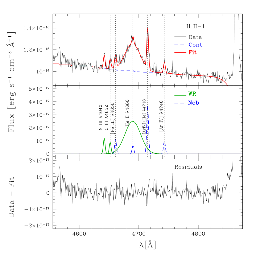
Figure 9.— Portion of the spectrum of H II-1 around the region of the Wolf-Rayet blue bump at $\sim$4690 Å. Top panel: Observed spectrum (thin black line) and total (continuum plus emission lines) fit (red thick line). The continuum has been modelled with a Z$=$0.004, 3-4 Myr old SSP, normalized at $4770-4840$ Å(see Section 5 for details). Middle panel: fitted emission lines (solid green line for WR features, dashed blue line for nebular narrow emission lines). Bottom panel: residual after subtracting the best-fit model.

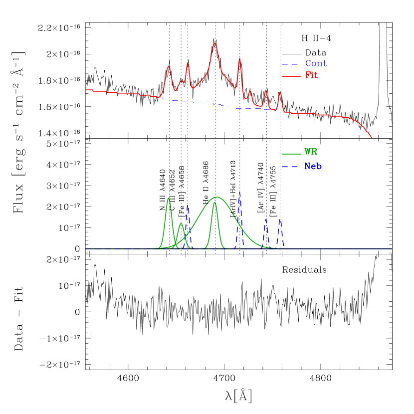
Figure 10.— Same as in Figure 9 but for H II-4.

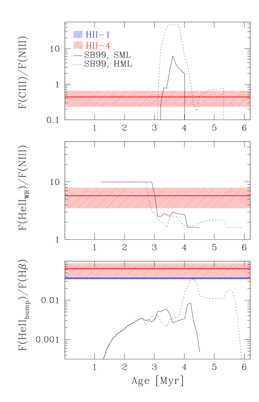
Figure 11.— Wolf-Rayet features detected in regions H II-1 and H II-4 against Starburst 99 (SB99) models. The models are based on the Geneva tracks with metallicity $Z=0.008$ with a standard mass-loss prescription (solid line) and with a high mass-loss prescription (dotted line). From top to bottom: F(C III)/F(N III), F(He II_WR)/F(N III), and F(He II_WR)/F(H$\beta$) ratios versus age. Notice that the F(He II_WR) flux refers to the broad WR component without the contribution from the nebular He II emission line.

We detected the blue bump in two (H II -1 and H II -4) out of the six H II regions studied in NGC 4449. On the other hand, the wavelength range of the red bump falls close to the region of low sensitivity of the blue and red MODS detectors, preventing us to draw conclusions about the presence of this feature. The blue bump spectral region in H II-1 and H II-4 was modeled by simultaneously fitting the WR features (N III $\lambda$4640, C III $\lambda$4652, He II $\lambda$4686) and the nebular emission lines ([Fe III] $\lambda$4658, He II $\lambda$4686, [Ar IV]$+$He I $\lambda$4713, [Ar IV]$\lambda$4740) following an approach similar to that of Brinchmann et al. (2008). To evaluate the underlying stellar continuum, we performed a spectral energy distribution (SED) fit to the 4000-7000 Å range (avoiding the regions contaminated by nebular emission lines) using SSP models from the Padova group (Marigo et al., 2008; Chavez et al., 2009). The SED of H II -1 and H II -4 turned out to be best reproduced by a Z$=$0.004, 3-4 Myr old population; this result, which we expect to be highly affected by the age-metallicity degeneracy, is not intended to draw conclusions on the physical properties of the underlying stars, but has the mere purpose of providing a reliable continuum below the bump. The fits to the blue bump in regions H II-1 and H II-4 are shown in Figures 9 and  10, respectively. We fixed the nebular emission lines to have the same Gaussian widths as the other emission lines in the 4000-6000 Å spectral range (FWHM$\sim$4 Å), while the FWHMs of the WR features were allowed to vary as free parameters.

For region H II-1, the width of the broad He II $\lambda$4686 feature is best fitted with a Gaussian FWHM of $\sim$30 Å, corresponding to a velocity $\sigma\sim$800 km s^-1 ; the presence of a nebular contribution to this line is not well constrained given the large errors (see Table 4). Surprisingly, the N III $\lambda$4640 and C III $\lambda$4652 features show widths comparable to those of the nebular emission lines. A similar result was found by Smith et al. (2016) when fitting the WR blue bump for cluster #5 in the blue compact dwarf galaxy NGC 5253; as they noticed, the narrow widths derived for N III and C III would suggest that these lines are likely to be nebular in origin, although detecting these transitions is unusual.

For region H II-4, it was necessary to assume two broad emission components to obtain a satisfactory fit to the He II $\lambda$4686 feature: our best fit provides two Gaussians with FWHMs of $\sim$8 Å and $\sim$ 45 Å, corresponding to velocities of $\sim$200 km s^-1 and $\sim$1200 km s^-1, while the N III and C III features are reproduced by two Gaussians with FWHM$\sim$8 Å. Notice that wind velocities derived in WR stars can be as high as $\sim$2500 km s^-1 (e.g., Niedzielski & Skorzynski, 2002).

We show in Figure 11 a comparison of the WR features in H II-1 and H II-4 against the Starburst99 instantaneous burst models (Leitherer et al., 2014). For region H II-1, we do not show the ratios involving the C III and N III emission because, as previously discussed, the narrow widths derived for these lines would suggest that they are nebular in origin and not due to WR stars. The plotted models were computed with the Geneva $Z=0.008$ stellar tracks (Schaller et al., 1992; Meynet et al., 1994) assuming either a standard mass-loss (SML) or a high mass-loss (HML) rate. It is well known that models of massive stars suffer uncertainties due to rotation (e..g Meynet & Maeder, 2005) and to possible binary evolution (e.g. Eldridge et al., 2008; Vanbeveren et al., 2007). Models including rotation have been computed by the Geneva group for some metallicities, but are not available for $Z=0.008$.

Figure 11 shows that WR features (mainly C III, N III and He II $\lambda$4686) are visible during a limited age range, from $\approx$1 Myr to $\approx$4.5 Myr in the case of SML models, and up to $\approx$6 Myr for HML models. While the N III emission is always present during the WR phase, the C III emission due to the later appearance of WC stars is observed only after $\approx$3 Myr (top panel of Fig. 11). This holds both for the SML and for the HML models, although we notice that the latter ones imply significantly higher F(C III)/F(N III) ratios. The presence of broad C III emission in H II-4 indicates the existence of a WR population at least $\approx$ 3 Myr old. The behaviour of the F(He II $\lambda$4686)/F(N III) ratio is displayed in the middle panel of Fig. 11. The SML and HML models predict a moderate difference in this ratio. The F(He II)/F(N III) ratio is as high as $\sim$10 in the earliest phases, and then rapidly decreases after $\sim$3 Myr reaching down to $\sim$2. For H II-4, we derive a ratio of $\sim 6\pm 2$, compatible with an age of $\sim$3 Myr. Finally, the bottom panel of Fig. 11 shows the evolution of the F(He II $\lambda$4686)/F(H$\beta$) ratio, which is proportional to the number of WR stars over the number of ionizing OB stars. Here the difference between the two sets of models is striking: while the SML largely under-predict the number of WR over OB stars, the HML provide a very satisfactory match for ages older than $\approx$4 Myr for both H II-1 and H II-4. This is in agreement with past studies in the literature showing that the observed properties of WR stars require, in absence of stellar models with rotation, the inclusion of an enhanced mass loss (e.g. Schaller et al., 1992; Schaerer & Maeder, 1992). However, we caution that the difficulty of the models in reproducing the strength of the blue bump could be due to the presence of stars other than “classical” WR, such as massive, mass losing core-hydrogen burning stars close to the main sequence, a stellar phase not yet accounted for in the evolution models (Leitherer et al., 2017). Using the HML models we derive, from the observed He II $\lambda$4686 flux, a number of WR stars of $\approx 4$ and $\approx 8\pm 2$ in regions H II-1 and H II-4, respectively.

6. Results on the Chemical Abundances and Abundance Ratios

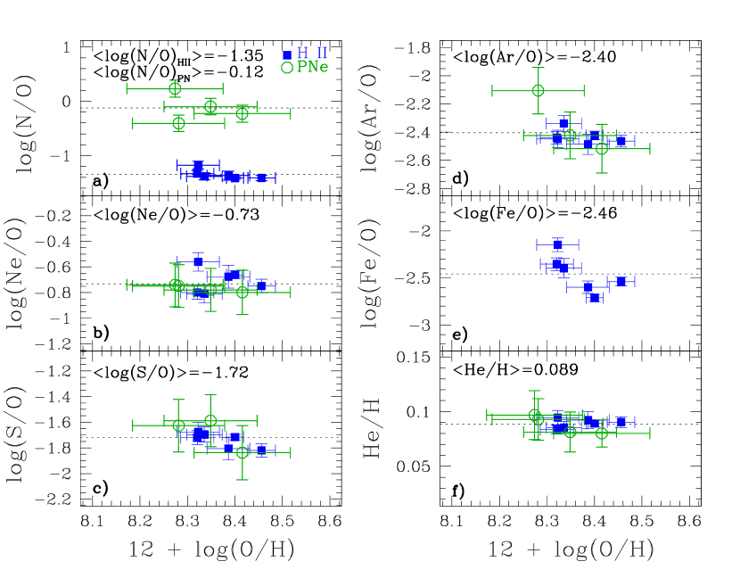
Figure 12.— Abundance ratios as a function of total oxygen abundance. Solid and open symbols are for H II regions and PNe, respectively. Within each panel, the label and the dotted horizontal line indicate the average value for the combined H II region and PN data; only in panel a), separate $\log(N/O)$ mean values for H II regions and PNe are provided.

Element abundances derived in H II regions and PNe are given in Tables 7 and 8. The oxygen abundance interval spanned by our sample is ${\rm 8.3\pm 0.1\leq 12+\log(O/H)\leq 8.46\pm 0.03}$, with average O abundances for H II regions and PNe of 8.37 $\pm$ 0.05 and 8.3 $\pm$ 0.1, respectively. The H II region results are consistent with previous literature measurements based on the direct temperature method: Talent (1980), see also Skillman et al. (1989), derived an average oxygen abundance of $12+\log(O/H)=8.31\pm 0.07$ for H II regions in NGC 4449; later, Berg et al. (2012) obtained new MMT spectra for the bright H II knot located a few arcsec to the south of our H II-6 region (slit 10 in Figure 1), and found an average abundance of $12+\log(O/H)=8.20\pm 0.08$, consistent with our value of $12+\log(O/H)=8.32\pm 0.04$ within the errors.

The trend of H II region and PN abundance ratios versus total oxygen abundance is illustrated in Figure 12. We find that, within the oxygen interval spanned by our data, the Ne/O, S/O and Ar/O ratios are similar for the H II region and PN sub-samples, and are compatible, within the errors, with a constant trend as a function of oxygen (Figs 12b, 12c and  12d). This behaviour is consistent with what is commonly observed in other studies (e.g., Richer & McCall, 2007; Bresolin et al., 2010; Stasińska et al., 2013; Annibali et al., 2015). The explanation is that $\alpha$-elements are all synthesized by massive stars on similar timescales, thus their abundance variations occur in lockstep, maintaining the corresponding ratios constant. The similarity between the Ne/O, S/O and Ar/O ratios measured in PNe and H II regions is not surprising since $\alpha$ - elements are not significantly affected during the evolution of low and intermediate mass stars. In NGC 4449, the average values of $<\log(Ne/O)>\simeq-0.73$, $<\log(S/O)>\simeq-1.72$, and $<\log(Ar/O)>\simeq-2.40$ are consistent with typical abundance ratios derived in H II regions of star-forming dwarf galaxies (see Figure 13 of Annibali et al., 2015, for NGC 1705).

The major abundance difference between H II regions and PNe is observed for Nitrogen (Figure 12a), showing a dichotomy in the N/O distribution. Our H II regions exhibit an average $<\log(N/O)_{H~{}II}>\simeq-1.35$, comparable to values measured in H II regions of luminous dwarf galaxies (e.g. Kobulnicky & Skillman, 1996; Berg et al., 2012) and of spirals for similar oxygen abundances as in NGC 4449 (e.g. Bresolin et al., 2009a; Berg et al., 2015; Croxall et al., 2016). On the other hand, our PNe are more than $\simeq$1 dex enhanced in N with respect to H II regions, with an average $<\log(N/O)_{PNe}>\simeq-0.12$. This is not unusual since previous studies have shown that PNe in nearby galaxies are enriched in N with respect to H II regions; there is a large scatter in the amount of the enrichment, with N/O ratios from close to those measured in H II regions up to $\approx$ 1 dex higher (e.g. Peña et al., 2007; Richer & McCall, 2007, 2008; Bresolin et al., 2010; Stasińska et al., 2013; García-Rojas et al., 2016). Highly N-enriched PNe are found both in star-forming galaxies and in quiescent early-type galaxies, where star formation ceased a long time ago (e.g. Richer & McCall, 2008). However, we notice that our PNe, despite their significant N enrichment, do not appear to be enhanced in He (Fig. 12f); to our knowledge, there are no models that can simultaneously increase the N abundance by a factor of 10 and leave He unchanged (see e.g. Karakas & Lattanzio, 2007). A possible explanation is that our derived PN He abundances are uncertain because the detected He I $\lambda 5876$ line is significantly fainter than two nearby sky lines at $\lambda\sim 5867$ Å and $\lambda\sim 5890$ Å.

From the theoretical point of view, the N/O enhancement in PNe is the natural consequence of nitrogen being mostly synthesized in intermediate mass stars, that are the PN progenitors, and brought to the stellar surface during dredge-up episodes occurring in the RGB and AGB phases; a significant N production may also occur in the most massive and luminous AGB stars through HBB (see Section 1). PNe exhibiting the most extreme N (and He) abundances, classified as type I, are thought to be the descendants of massive ($>$ 3 $M_{\odot}$), relatively young (age$\lesssim$400 Myr) AGB stars experiencing HBB (e.g. Stanghellini et al., 2006; Corradi & Schwarz, 1995). Torres-Peimbert & Peimbert (1997) proposed $\log(N/O)>-0.42$ and He/H$>0.105$ as an empirical criterion to select type I systems; three PNe out of four in our sample satisfy the condition in N/O, but their helium abundances are similar to those of H II regions around He/H$\simeq$0.09 (see Figure 12f), which can not be explained with existing models. Although the reliability of the derived He abundances for our PNe could be questioned as discussed before, a strong selection bias should be invoked to explain why a fraction as high as 3/4 of our sample derives from massive star progenitors.

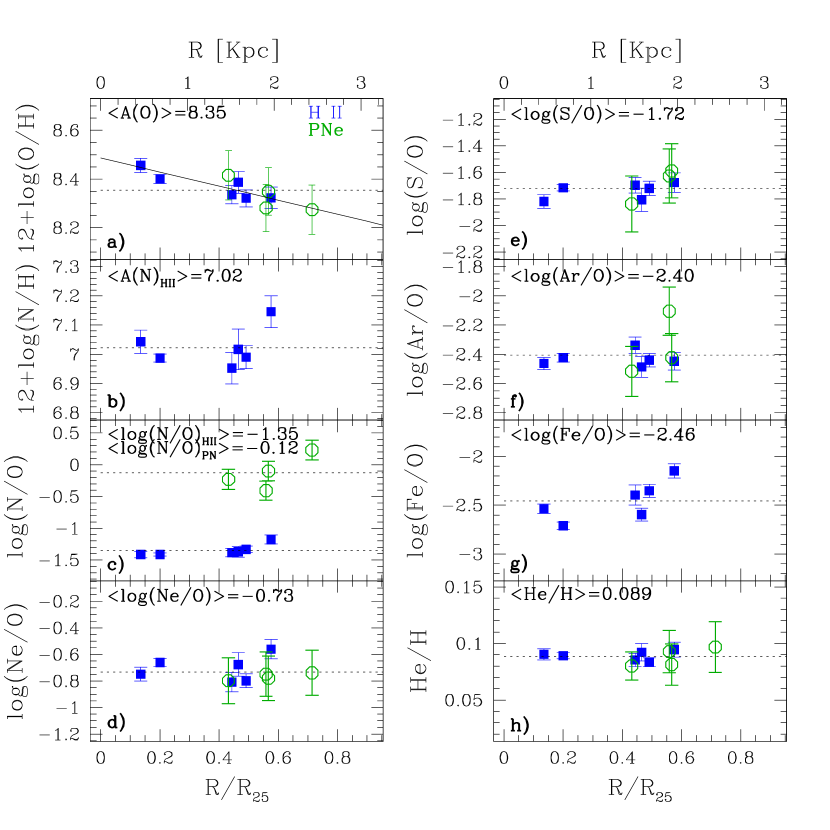
Figure 13.— Element abundances and abundance ratios as a function of galacto-centric distance $R/R_{25}$, where $R_{25}=3.4$ kpc. The linear galacto-centric scale in kpc is also indicated on top. Solid and open symbols are for H II regions and PNe, respectively. Within each panel, the label and the dotted horizontal line indicate the average value for the combined H II region and PN data; only in panel c), separate $\log(N/O)$ mean values for H II regions and PNe are provided. In panel b), in order to better visualise the range of nitrogen variation as a function of radius for H II regions, we do not include PNe, whose N abundance is so high (see Table 8) that the ordinate scale would be too compressed.

We find no significant trends in the N/O vs O/H distribution of Figure 12a. Historically, the absence of a trend in N/O vs O/H for low-metallicity systems was taken as the first indication that nitrogen cannot be a pure secondary element. Primary elements (like He, C and O) are those whose production can start already in stars with primordial initial chemical composition. Secondary elements are those that can be synthesized only if the star already contains their seed elements at birth or at the evolutionary phase when the physical conditions allow the element to be synthesized. As a natural consequence, the abundance of secondary elements is predicted to increase as the square of primary ones (Tinsley, 1980). Hence, had N been of fully secondary nature, its ratio to oxygen should have been proportional to the O abundance. Since N/O is instead always found to be quite independent of O/H in the nebulae of individual galaxies (see, e.g. Diaz & Tosi, 1986), a significant fraction of N must be of primary origin. In practice, its nature depends on whether the C used to synthesize N was produced by previous nuclear reactions in the same star or was already present in its initial chemical composition. An inspection of the chemical yields computed for low- and intermediate-mass stars (see e.g. Karakas, 2010; Ventura et al., 2013; Vincenzo et al., 2016) shows that N is mainly of secondary origin above a metallicity $\approx$ half of solar, and is mainly produced by M$\;\lower 2.58334pt\hbox{$\sim$}\kern-7.75pt\raise 2.79857pt\hbox{$>$}\;3.5M_{\odot}$ stars experiencing HBB (see also Figs 1 and 2 in Romano et al., 2010). In massive stars N can have a significant primary origin if their metallicity is low and they rotate sufficiently fast (Meynet & Maeder, 2002).

Finally, the distribution of the Fe abundance, derived only for H II regions, is shown in Figure 12e. The Fe/O ratio shows no clear trend with oxygen: in fact, although there is a hint for an Fe/O decrease with increasing O abundance, in agreement with the behaviour revealed by other studies (e.g., Izotov et al., 2006; Guseva et al., 2011; Delgado-Inglada et al., 2011) and commonly interpreted as Fe depletion into dust grains, the range in oxygen abundance probed by our data is likely too small to claim a clear trend. In particular, we notice that the data in the Fe/O versus O plane shown by Delgado-Inglada et al. (2011) span an oxygen interval of almost $\sim$2 dex, compared to a range of only $\sim$0.2 dex for the NGC 4449 data. Our Fe and O abundances nicely fall upon the region occupied by H II regions in the Delgado-Inglada et al. (2011) plot.

7. Results on the abundance spatial distributions

The behaviour of element abundances as a function of galacto-centric distance is shown in Figure 13. For immediate comparison between NGC 4449 and other literature studies, the radial distance is expressed in terms of $R/R_{25}$, where the optical isophotal radius $R_{25}=3.1^{\prime}$ is taken from Pilyugin et al. (2015), and corresponds to $\approx$3.4 kpc at NGC 4449’s distance of $\approx$ 3.8 Mpc.

Figure 13a shows that H II regions and PNe exhibit similar oxygen abundances in the galacto-centric distance range of overlap, despite the fact that they represent different evolutionary stages of the galaxy. The same result was found for other star-forming dwarf and spiral galaxies by previous studies reporting similar abundances for H II regions and bright PNe (e.g. Richer, 1993; Magrini et al., 2005; Richer & McCall, 2007; Bresolin et al., 2010; Stasińska et al., 2013). From the analysis of the CMD of the resolved stars, we know that NGC 4449 has been actively forming stars over the last 1 Gyr (Annibali et al., 2008; McQuinn et al., 2010; Sacchi et al., 2017); therefore we would expect a significant chemical enrichment since the PN progenitors were formed, i.e. since $\sim$100 Myr ago or more. On the other hand, the similarity in oxygen abundance between H II regions and PNe suggests that this is not the case. The galactic outflow observed in NGC 4449 (Della Ceca et al., 1997; Summers et al., 2003; Bomans & Weis, 2014) may have played an important role, expelling the recently produced $\alpha$-elements. Accretion of metal poor gas or acquisition of smaller gaseous systems may have also contributed to dilute the metals in the ISM.

Figure 13a illustrates that both H II regions and PNe show a well-defined oxygen gradient. We thus combined H II and PN data to infer a global relation from a linear least-squares fit:

$${\rm 12+\log(O/H)=-0.29(\pm 0.06)\times R/R_{25}+8.49(\pm 0.030)}.$$ (15)

Hence our gradient is ${\rm(-0.29\pm 0.08)\ dex\ R_{25}^{-1}}$ , in good agreement with the value of ${\rm(-0.23\pm 0.03)\ dex\ R_{25}^{-1}}$ obtained by Pilyugin et al. (2015), once we correct his O/H gradient for the larger distance adopted in his work (${\rm D_{NGC~{}4449}\approx 4.1\ Mpc)}$. On the other hand, we notice that the central extrapolated oxygen abundance derived by Pilyugin et al. (2015) is $12+\log(O/H)=8.26\pm 0.01$, more than 0.2 dex lower than ours.

The presence of metallicity gradients in late-type dwarf galaxies has been widely discussed in the literature. For a long time, dIrrs and BCDs have been considered to have nearly constant radial trends, at least within the observational uncertainties (e.g., Kobulnicky & Skillman, 1997; Croxall et al., 2009; Lagos & Papaderos, 2013; Haurberg et al., 2013). Two possible explanations have been proposed for this behaviour: (a) the ejecta from stellar winds and supernovae are dispersed and mixed across the ISM on short timescales, of the order of $\lesssim 10^{7}$ year; (b) freshly synthesized elements remain unmixed with the surrounding ISM and reside in a hot $10^{6}$ K phase or a cold, dusty, molecular phase (Kobulnicky & Skillman, 1997). However, detections of negative metallicity gradients from stars and H II regions have been reported in the literature for the dIrr NGC 6822 (Venn et al., 2004; Lee et al., 2006), and spectroscopic studies of individual RGB stars have shown slightly negative gradients in [Fe/H] for the SMC, the LMC, and the dIrr WLM (Leaman et al., 2014, and references therein). Very recently, our study of the BCD NGC 1705 (Annibali et al., 2015) and the study by Pilyugin et al. (2015) showed that negative nebular metallicity gradients are indeed present in late-type dwarf galaxies; our results for NGC 4449 reinforce this scenario. We suspect that these recent studies were able to reveal gradients previously undetected thanks to the high-quality data implied, allowing for much smaller uncertainties on the element abundance determinations.

Figures 13d, 13e, and 13f show a constant trend of the Ne/O, S/O, and Ar/O abundance ratios with galacto-centric distance, which, as described in Section 6, is expected because $\alpha$-elements are all synthesized by massive stars on similar timescales and vary in lockstep. Also the He abundance remains constant with galacto-centric distance (Figure 13h), in agreement with the absence of any trend of He with oxygen in Figure 12f. On the other hand, Fe/O decreases with increasing galacto-centric distance (Figure 13g), which is expected from the presence of an oxygen radial gradient and from the fact that Fe/O decreases with increasing O in Figure 12e.

Figure 13b and  13c show the radial distribution of the N abundance and of the N/O ratio, respectively. The behaviour of nitrogen in Figures 13b and  13c deserves particular discussion. In fact, despite the existence of a well-defined oxygen metallicity gradient in Figure 13a, no clear trend of the N abundance with galacto-centric distance is observed for H II regions. This behaviour is surprising, since we expect that the present ISM in NGC 4449 contains a significant component of secondary N (see e.g. Vincenzo et al., 2016), implying that an oxygen metallicity gradient should be accompanied by a nitrogen gradient at least as steep (see for instance studies of spiral galaxies, e.g. Diaz & Tosi, 1986; Bresolin et al., 2009a; Croxall et al., 2015).

Given the evidence for a conspicuous population of WR stars in NGC 4449 (Martin & Kennicutt, 1997; Bietenholz et al., 2010; Srivastava et al., 2014; Sokal et al., 2015, see also Section 5), local pollution from WR ejecta enriched in N is an attractive possibility to explain the observed behaviour. Although significant amounts of N and C are expected to be injected by WR stars on theoretical grounds (e.g. Chiosi & Maeder, 1986; Dray & Tout, 2003; Meynet & Maeder, 2005), observational results have been discrepant so far, suggesting either the absence (Kobulnicky & Skillman, 1996; Kobulnicky, 1999b) or the presence (Kobulnicky et al., 1997; López-Sánchez et al., 2007, 2011; James et al., 2011, 2013) of localised metal enrichment by massive star ejecta. A proposed explanation for these ambiguous results is that an N/O excess is observed only after a recently completed WR phase, when the WR features are weak and the ejecta have cooled. In this picture, strong WR features trace very young regions where the stellar ejecta are still in a hot (T$\approx 10^{6}$ K) phase and do not show up in optical spectroscopy of H II regions (Tenorio-Tagle, 1996; Wofford, 2009). This scenario is supported by a study of a large galaxy sample from the SDSS (Brinchmann et al., 2008) where an excess in N/O is found for WR galaxies with EW(H$\beta$)$<$100 Å (i.e. burst ages  $\sim$$>$ 6 Myr), while WR and non-WR galaxies do not show difference in N/O for EW(H$\beta$)$>$100 Å (i.e. burst ages $\lesssim$6 Myr). Indeed, the two regions with strong WR features in our sample (H II-1 and H II-4) do not exhibit particularly high N/O values, while H II-6, which does not have WR features but is located in a region of very active SF, presents an N/O excess. Whether there is a correlation in NGC 4449 between the age of the burst and the N abundance for the individual H II regions will be investigated in a forthcoming paper (Sacchi et al., 2017) based on UV LEGUS data (Calzetti et al., 2015).

8. Distinctive properties of the PN population

Further insights on the overall evolutionary status of the PNe in NGC 4449 can be attained by considering the full sample of 28 bona fide candidates examined either with spectroscopic or with photometric observations (see Table 9). The statistics is affected by a selection bias, since our PN detection is restrained only to the most active objects with prominent [O III] emission at 5007 Å (for the target to clearly stand out in the $V$ or F502N band frames, compared to $B$ and $I$ imaging). Notice that younger stars do not produce brighter [O III] planetary nebulae; however, at NGC 4449’s metallicity and lower, the highest luminosity that a PN can attain increases with increasing oxygen abundance (Dopita et al., 1992; Richer, 1993). Therefore, we can not exclude that our selection criterium has picked-up only the most oxygen-rich PNe in NGC 4449.

Within the biased and limited size of our sample, a preliminary, yet useful, estimate of the luminosity-specific PN number density $\alpha=N_{PN}/L_{gal}$ (Jacoby, 1980) may be attempted. This parameter directly relates the amount of light in a stellar system to be associated to any observed PN sample, and it closely traces the distinctive evolutionary properties of the underlying stellar population in the parent galaxy. For this task we first require an estimate of NGC 4449 bolometric luminosity, followed by a quantitative assessment of the completeness factor of our PN counts.

Table 9The total sample of 28 PNe.

ID	mF555W	mF502N	$(M-M^{*})_{[OIII]}$	ID	mF555W	mF502N	$(M-M^{*})_{[OIII]}$
	[Vega mag]	[Vega mag]	[mag]		[Vega mag]	[Vega mag]	[mag]
PN-1	23.86	$-$	0.82	PN-15	25.41	22.85	2.36
PN-2	24.39	$-$	1.01	PN-16	25.49	23.10	2.44
PN-3	24.46	22.03	1.25	PN-17	24.57	22.00	1.52
PN-4	24.78	22.6	0.57	PN-18	23.82	21.85	0.77
PN-5	24.26	$-$	1.01	PN-19	23.38	21.83	0.33
PN-6	24.33	22.02	1.28	PN-20	23.63	21.60	0.58
PN-7	24.47	22.38	1.42	PN-21	24.27	22.69	1.22
PN-8	25.11	22.72	2.06	PN-22	24.89	22.19	1.84
PN-9	24.62	22.48	1.57	PN-23	24.34	21.89	1.29
PN-10	24.51	22.18	1.46	PN-24	23.29	21.30	0.24
PN-11	24.20	21.85	1.15	PN-25	25.15	23.16	2.10
PN-12	23.96	21.56	0.91	PN-26	24.70	21.99	1.65
PN-13	23.93	21.57	0.88	PN-27	23.09	20.75	0.04
PN-14	25.59	22.93	2.54	PN-28	24.97	22.30	1.92

Note. — Apparent m_F555W and m_F502N magnitudes derived for our sample of 28 PNe from HST/ACS data. The $(M-M^{*})_{[OIII]}$ magnitude difference for PN-1 to PN-5 is obtained from the observed $[OIII]$ fluxes listed in Table 5 (corrected for the distance modulus), by assuming $M^{*}_{[OIII]}=-4.36$ as the PN cutoff-magnitude. For the remaining objects, we nominally assume $m_{[OIII]}=m_{F555W}+0.5$, as explained in the text.

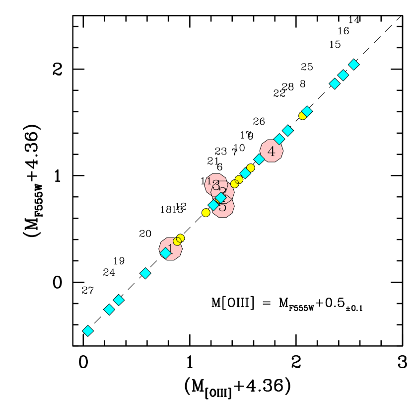
Figure 14.— The $M_{F555W}$ magnitudes of the spectroscopic PN sample are compared to the corresponding $M_{[O~{}III]}$ values (big dot markers). All magnitudes have been corrected for the distance modulus and offset by a value of $+4.36$ mag, corresponding to the PNLF bright cutoff magnitude ($M^{*}_{[O~{}III]}$). A straight relationship is in place with $M_{[O~{}III]}-M_{F555W}=0.5\pm 0.1$. When applied to the total photometric PN sample (diamond markers), this offset allows us to assess the $M_{[O~{}III]}$ distribution of the whole sample of 28 PNe showing that our observations actually probed the bright tail of NGC 4449 PNLF, down to $(M_{[O~{}III]}-M^{*}_{[O~{}III]})\sim 2.5$ mag. In the plot each nebula is labeled according to its entry ID of Table 9.

The apparent integrated magnitude $V^{N4449}_{o}=9.47\pm 0.3$ and the color $(B-V)^{N4449}_{o}=0.36\pm 0.07$ of NGC 4449 are taken from the corresponding RC3 (de Vaucouleurs et al., 1991) and Gronwall et al. (2004) entries, assuming a Galactic foreground reddening of $E(B-V)=0.019$ (Schlegel, Finkbeiner, & Davis, 1998). A match of these figures with the Buzzoni (2005) Im template galaxy model (see Table A7 therein) suggests a bolometric correction in the range $(Bol-V)=-0.84\pm 0.02$, from which an absolute value of $M_{bol}=-19.3\pm 0.3$ and a total bolometric luminosity of $L=(4.0\pm 1.0)\,10^{9}~{}L_{\odot}$ can be obtained, once accounting for the galaxy distance modulus, and assuming for the Sun $M^{bol}_{\odot}=+4.72$ (Lang, 1980).

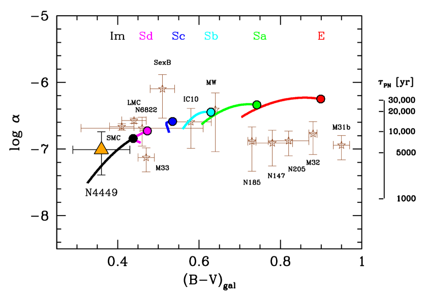
Figure 15.— A comprehensive overview of the derived luminosity-specific PN number density $\alpha$ for NGC 4449, compared with Local Group galaxies (star markers) as from Buzzoni, Arnaboldi, & Corradi (2006). Also superposed are the Buzzoni (2005) template galaxy models along the whole morphological sequence from 2 to 15 Gyr, with the latter limit marked by the big solid dots. The Weidemann (2000) empirical scheme is adopted for properly assessing stellar mass loss in the galaxy models. An indicative estimate of the mean representative PN visibility timescale (in years) is sketched on the right scale, as discussed in the text.

Our PN completeness level can be estimated by relying on the classical Henize & Westerlund (1963) PN luminosity function (PNLF), in the form of an exponential curve with a sharp truncation designed to accomodate the bright end (cf. e.g. Ciardullo et al., 1989; Jacoby & De Marco, 2002). An absolute $M_{[O~{}III]}$ magnitude (at 10 pc) can be derived for each nebula in our spectroscopic sample, according to the observed [O III] flux of Table 3, corrected for the distance modulus of $(m-M)_{0}\sim 27.9$ (Annibali et al., 2008), as $M_{[O~{}III]}=-2.5\,\log F_{[O~{}III]}-13.74$. These figures can be contrasted with the bright cut-off magnitude (M${}^{*}_{[O~{}III]}$) of Ciardullo et al. (1989) PNLF that, for the NGC 4449 metallicity, can be set at $M^{*}_{[O~{}III]}=-4.36$ (Ciardullo et al., 2002). Our results are summarized in Table 9 and Fig. 14.

The figure also provides a mapping between $M_{F555W}$ magnitudes and $M_{[O~{}III]}$ magnitudes for the five planetary nebulae with spectroscopy. For this task we relied on the observed $m_{F555W}$ magnitudes, after correcting the Table 9 entries for distance modulus. As expected, the $M_{F555W}$ magnitude of the five spectroscopic nebulae happens to be a quite confident proxy of the corresponding $M_{[O~{}III]}$, with $M_{[O~{}III]}=M_{F555W}+0.5\pm 0.1$ (see Fig. 14). When applied to the remaining photometric targets, one can therefore conclude that our observations sample the bright tail of NGC 4449 PNLF, down to $(M_{[O~{}III]}-M^{*}_{[O~{}III]})\sim 2.5$ mag.

Adopting the standard PNLF, as scaled for instance from the M31 (Ciardullo et al., 1989) or LMC observations (Reid & Parker, 2010) down to $\sim 8$ mag fainter than the bright cut-off limit $M^{*}_{[O~{}III]}$, we obtain a total expected number of $280\pm 53$ (Poissonian rms) PNe for our field. A lower value of $\sim 145\pm 27$ would be obtained assuming instead the SMC PNLF, as from the deep [O III]₅₀₀₇ observations of Jacoby & De Marco (2002). These values need to be corrected for the fact that we are missing the PNe in the most crowded, central $R/R_{25}\lesssim 0.1$ galaxy regions: adopting the galaxy surface brightness profile of Rich et al. (2012), we estimate a $\sim$40 % correction to the PN number, which translates into $392\pm 74$ for an assumed Ciardullo et al. (1989) PNLF (or $203\pm 38$ PNe assuming the SMC PNLF). We caution that these estimates are highly uncertain because our extrapolation assumes that our sample is proportional to the complete sample from the brightest PN down to $\sim$2.5 mag below the PNLF cutoff; indeed a robust determination of the PN completeness as a function of magnitude would require artificial star tests performed on the images, which is beyond the scope of this paper.

With these figures, our estimate of the $\alpha$ parameter leads eventually to

$$\log\alpha=\log\left[\frac{392_{\pm 74}}{4.0_{\pm 0.1}\,10^{9}}\right]=-7.01^{+0.27}_{-0.38},$$ (16)

to which, in addition to the Poissonian error from the counts, we attached an uncertainty range that either assumes a 50% fraction of PNe in excess due to a more conservative completeness limit at $\sim 1.5$ mag below the bright cutoff or, conversely, a halved reduction of the PN number, as from the Jacoby & De Marco (2002) SMC PNLF.

A comparison with other Local Group galaxies is shown in Fig. 15, following Buzzoni, Arnaboldi, & Corradi (2006). In the plot we also report the theoretical predictions for Buzzoni (2005) template galaxy models, between 2 and 15 Gyr, according to Weidemann’s (2000) stellar mass-loss scheme. The models predict that $\alpha$ decreases in young and/or star-forming galaxies, compared to more quiescent early-type systems as a consequence of a smaller population of PNe embedded in a higher galaxy luminosity per unit mass (i.e. a lower M/L ratio). We notice that the luminosity-specific PN number in NGC 4449, as well as the values derived for other late-type systems, agree quite well with the Buzzoni (2005) models (on the other hand, the models are less successful for the earliest galaxy types).

From a theoretical point of view, the luminosity-specific PN number density easily relates with the reference visibility lifetime ($\tau_{PN}$) of the PN events, being $\alpha={\cal{B}}\times\tau_{PN}$, with $\cal{B}$ the so-called specific evolutionary flux of a stellar population (see Buzzoni, Arnaboldi, & Corradi, 2006, for the theoretical background). The PN visibility lifetime $\tau_{PN}$ depends both on the chemical and dynamical properties of the ejected material, and on the stellar core evolution during the PAGB phase. In general, for young and intermediate-age SSPs, the PAGB timescale ($\tau_{PAGB}$) is shorter than the dynamical time-scale for the nebula evaporation, so that the PN lifetime might likely be shorter for more massive, and younger, stellar progenitors. This trend is schematically sketched in Fig. 15 relying on Buzzoni, Arnaboldi, & Corradi (2006) theoretical framework. According to these models, the typical visibility lifetime for the PNe in NGC 4449 is predicted to be a few thousand years.

9. Conclusions

We presented new deep multi-object spectroscopy with LBT/MODS of H II regions and PNe in the starburst irregular galaxy NGC 4449, at a distance of $\approx$3.8 Mpc from us. The [O III]$\lambda 4363$ auroral line was detected in all spectra, allowing for a direct determination of the O⁺² temperature. For the H II regions, the O⁺ and S⁺² temperatures were also derived from the [O II]$\lambda 7320+\lambda 7330/\lambda 3726+\lambda 3729$ and [S III]$\lambda 6312/\lambda 9069+\lambda 9532$ ratios. Using the “direct” method, we derived the abundance of He, N, O, Ne, Ar, and S for six H II regions and, for the first time, for four PNe in NGC 4449. Iron abundances were also derived for the H II regions, but this element is notoriously highly affected by depletion into dust grains. The combined H II region and PN sample covers a galacto-centric distance range of $\sim$2 kpc, corresponding to $\approx$70% of the $R_{25}$ isophotal radius. Our main results are:

1. The total H II region $+$ PN sample spans $\sim$0.2 dex in oxygen abundance, with average $12+\log(O/H)$ values of 8.37 $\pm$ 0.05 and 8.3 $\pm$ 0.1 for H II regions and PNe, respectively. The results for the H II regions are consistent, within the errors, with previous literature estimates based on the direct temperature method.

2. We find a well defined trend of decreasing oxygen abundance with increasing galacto-centric distance: $12+\log(O/H)=-0.29(\pm 0.06)\times R/R_{25}+8.49(\pm 0.030)$, with H II regions and PNe exhibiting similar oxygen abundances at the same galacto-centric distance. This result, coupled with our previous finding of a negative metallicity gradient for H II regions in the blue compact dwarf NGC 1705 (Annibali et al., 2015) and with the recent results by Pilyugin et al. (2015), suggests that metallicity gradients do exist in irregular galaxies, at odds with what was previously believed (e.g. Kobulnicky & Skillman, 1997; Croxall et al., 2009; Haurberg et al., 2013; Lagos & Papaderos, 2013).

3. Despite the presence of a negative oxygen gradient, nitrogen does not exhibit any well-defined radial trend. This is unexpected, since an important component of secondary nitrogen should exist in the present-day ISM of NGC 4449. Building on previous literature studies showing evidence for N/O inhomogeneities in Wolf-Rayet galaxies, we suggest that the anomalous nitrogen behaviour may be due to local enrichment by the conspicuous Wolf-Rayet population in NGC 4449.

4. The studied PNe exhibit a significant nitrogen enhancement with respect to H II regions ( $\sim$$>$ 1 dex); this behaviour is in agreement with previous chemical abundance studies of PNe in galaxies of different morphological types. On the other hand, we also find that the PN helium abundances are similar to those of NGC 4449’ s H II regions, around He/H$\simeq$0.09 (although we caution that our PN He estimates are very uncertain because the detected He I $\lambda 5876$ line is significantly fainter than two nearby sky lines at $\lambda\sim 5867$ Å and $\lambda\sim 5890$ Å). From the theoretical point of view, we expect both N and He to be enhanced in PNe because they are both synthesized and brought to the stellar surface through dredge-up episodes occurring in the RGB and AGB phases of intermediate mass stars. We are not aware of any model producing a factor $\sim$10 enhancement in N while leaving He unchanged.

5. Our PN oxygen (and $\alpha$-element, more in general) abundances are, on the other hand, similar to those of H II regions in the galacto-centric distance range of overlap. This indicates that the NGC 4449’s ISM has not been significantly enriched in metals since the progenitors of the PNe were formed (i.e., since $\sim$ 100 Myr ago or more). Recently produced $\alpha$-elements may have been expelled from NGC 4449 by the galactic outflow, or may still reside in a hot phase (see e.g. Martin et al., 2002, for NGC 1569); also, acquisition of metal poor gas may have diluted the metals in the ISM.

6. The derived luminosity-specific PN number density ($\alpha=N_{PN}/L_{gal}$) in NGC 4449 agrees quite well with the Buzzoni (2005) template galaxy models that predict the behaviour of $\alpha$ as a function of galaxy morphological type and color; according to these models, the $\alpha$ value derived in NGC 4449 translates into a typical visibility lifetime for the PN population of a few thousand years.

7. Two out of the six studied H II regions show broad emission features associated with Wolf-Rayet stars of WN and WC subtypes. From a comparison with population synthesis models, we infer that a WR population at least 3$-$4 Myr old must be present in NGC 4449.

Appendix A H II regions and PNe spectra

We present the LBT/MODS spectra of H II regions H II-2, H II-3, H II-4, H II-5, H II-6 in Figures 16, 17, 18, 19, 20, respectively, and of planetary nebulae PN-2, PN-3, PN-4, PN-5 in Figures 21, 22, 23, 24, respectively.

Figure 16.— LBT/MODS spectra in the blue and red channels for H II-2 in NGC 4449 with indicated all the identified emission lines. The spectra have been scaled such that the details are evident.

Figure 17.— Same as Fig. 16 but for H II-3.

Figure 18.— Same as Fig. 16 but for H II-4.

Figure 19.— Same as Fig. 16 but for H II-5.

Figure 20.— Same as Fig. 16 but for H II-6. The small insertion provides a zoom into the $\sim$4640 - 4710 Å wavelength range to highlight the faint [Fe III]$\lambda$4658 and He II$\lambda$4686 lines.

Figure 21.— LBT/MODS spectra in the blue and red channels for PN-2 in NGC 4449 with indicated all the identified emission lines. A $\sim$1 Å boxcar filter smoothing was applied to the spectrum to better highlight the low singal-to-noise features. The spectra have been scaled such that the details are evident.

Figure 22.— Same as Fig. 21 but for PN-3.

Figure 23.— Same as Fig. 21 but for PN-4.

Figure 24.— Same as Fig. 21 but for PN-5.

Appendix B “Raw” emission line fluxes

We provide in Tables 2 and  3 the measured emission line fluxes, with no reddening correction applied, for our studied H II regions and PNe in NGC 4449. The reported flux values were obtained by averaging the results from different measurements, as outlined in Section 3; the associated uncertainties were simply obtained as the standard deviation of the different measurements. Notice that these errors do not account for additional uncertainties due to e.g. flux calibration.

Table 2Observed emission fluxes for H II regions in NGC 4449

Line	H II-1	H II-2	H II-3	H II-4	H II-5	H II-6
[O II] $\lambda$3727	23.69 $\pm$ 0.02	42.85 $\pm$ 0.04	75 $\pm$ 2	43.62 $\pm$ 0.04	24.70 $\pm$ 0.03	10.2 $\pm$ 0.1
H10 $\lambda$3978	1.41 $\pm$ 0.01	1.41 $\pm$ 0.02	1.19 $\pm$ 0.01	1.17 $\pm$ 0.01	0.60 $\pm$ 0.01	0.13 $\pm$ 0.01
He I $\lambda$3820	0.210 $\pm$ 0.001	0.163 $\pm$ 0.001	$-$	0.110 $\pm$ 0.001	$-$	$-$
H9$+$He II $\lambda$3835	1.99 $\pm$ 0.01	1.907 $\pm$ 0.006	1.65 $\pm$ 0.01	1.63 $\pm$ 0.01	0.837 $\pm$ 0.002	0.195 $\pm$ 0.001
[Ne III] $\lambda$3869	7.22 $\pm$ 0.02	5.32 $\pm$ 0.01	2.64 $\pm$ 0.01	4.08 $\pm$ 0.01	1.96 $\pm$ 0.01	0.75 $\pm$ 0.01
H8$+$He I $\lambda$3889	4.33 $\pm$ 0.02	4.96 $\pm$ 0.01	3.81 $\pm$ 0.01	3.90 $\pm$ 0.01	2.19 $\pm$ 0.02	0.45 $\pm$ 0.01
H$\epsilon$ $+$ He I $+$[Ne III] $\lambda$3970	5.72 $\pm$ 0.01	5.44 $\pm$ 0.01	4.08 $\pm$ 0.01	4.84 $\pm$ 0.04	2.56 $\pm$ 0.03	0.64 $\pm$ 0.01
He I $\lambda$4026	0.462 $\pm$ 0.006	0.420 $\pm$ 0.004	0.18 $\pm$ 0.01	0.284 $\pm$ 0.001	0.105 $\pm$ 0.004	$-$
[S II] $\lambda$4068	0.168 $\pm$ 0.005	0.184 $\pm$ 0.002	0.50 $\pm$ 0.01	0.177 $\pm$ 0.002	0.143 $\pm$ 0.004	0.088 $\pm$ 0.001
[S II] $\lambda$4076	0.049 $\pm$ 0.008	0.095 $\pm$ 0.001	0.155 $\pm$ 0.002	$-$	$-$	0.034 $\pm$ 0.002
H$\delta$ $\lambda$4101	6.08 $\pm$ 0.01	6.96 $\pm$ 0.01	5.96 $\pm$ 0.04	6.10 $\pm$ 0.03	3.36 $\pm$ 0.04	0.69 $\pm$ 0.01
H$\gamma$ $\lambda$4340	10.93 $\pm$ 0.01	12.54 $\pm$ 0.01	10.46 $\pm$ 0.01	9.75 $\pm$ 0.01	5.74 $\pm$ 0.04	1.25 $\pm$ 0.01
[O III] $\lambda$4363	0.51 $\pm$ 0.02	0.460 $\pm$ 0.005	0.289 $\pm$ 0.004	0.310 $\pm$ 0.003	0.222 $\pm$ 0.004	0.059 $\pm$ 0.001
He I $\lambda$4389	0.137 $\pm$ 0.003	0.098 $\pm$ 0.003	$-$	0.096 $\pm$ 0.002	$-$	$-$
He I $\lambda$4471	1.03 $\pm$ 0.01	1.15 $\pm$ 0.01	0.70 $\pm$ 0.01	0.81 $\pm$ 0.01	0.39 $\pm$ 0.01	0.07 $\pm$ 0.01
[N III](WR) $\lambda$4640	0.046 $\pm$ 0.002	$-$	$-$	0.23 $\pm$ 0.01	$-$	$-$
[C III](WR) $\lambda$4652	0.028 $\pm$ 0.007	$-$	$-$	0.10 $\pm$ 0.03	$-$0	$-$
[Fe III] $\lambda$4658	0.034 $\pm$ 0.006	0.078 $\pm$ 0.001	0.186 $\pm$ 0.004	0.090 $\pm$ 0.007	0.060 $\pm$ 0.001	0.036 $\pm$ 0.004
He II (WR) $\lambda$4686	0.89 $\pm$ 0.04	$-$	$-$	1.33 $\pm$ 0.09	$-$	$-$
He II $\lambda$4686	0.10 $\pm$ 0.08	$-$	$-$	$-$	$-$	0.022 $\pm$ 0.001
[Ar IV]$+$He I $\lambda$4713	0.12 $\pm$ 0.01	0.107 $\pm$ 0.001	$-$	0.11 $\pm$ 0.01	$-$	$-$
[Ar IV] $\lambda$4740	0.041 $\pm$ 0.003	$-$	$-$	0.064 $\pm$ 0.009	$-$	$-$
H$\beta$ $\lambda$4861	25.02 $\pm$ 0.02	29.06 $\pm$ 0.01	22.77 $\pm$ 0.04	21.76 $\pm$ 0.03	12.42 $\pm$ 0.01	2.72 $\pm$ 0.01
He I $\lambda$4922	0.30 $\pm$ 0.01	0.35 $\pm$ 0.01	0.17 $\pm$ 0.01	0.23 $\pm$ 0.02	0.10 $\pm$ 0.01	$-$
[O III] $\lambda$4959	36.190 $\pm$ 0.005	38.200 $\pm$ 0.008	16.37 $\pm$ 0.02	22.95 $\pm$ 0.06	14.010 $\pm$ 0.005	2.913 $\pm$ 0.006
[Fe III] $\lambda$4986	0.049 $\pm$ 0.004	0.11 $\pm$ 0.01	0.268 $\pm$ 0.005	0.084 $\pm$ 0.001	0.073 $\pm$ 0.003	0.054 $\pm$ 0.001
[O III] $\lambda$5007	106.40 $\pm$ 0.01	113.50 $\pm$ 0.01	48.22 $\pm$ 0.03	67.35 $\pm$ 0.02	40.37 $\pm$ 0.01	8.45 $\pm$ 0.01
He I $\lambda$5015	0.624 $\pm$ 0.004	0.804 $\pm$ 0.003	0.50 $\pm$ 0.01	0.52 $\pm$ 0.02	0.273 $\pm$ 0.002	0.062 $\pm$ 0.005
[N I] $\lambda$5199	0.054 $\pm$ 0.001	0.041 $\pm$ 0.001	0.243 $\pm$ 0.006	0.059 $\pm$ 0.002	0.044 $\pm$ 0.001	0.064 $\pm$ 0.001
He I $\lambda$5876	3.14 $\pm$ 0.01	4.04 $\pm$ 0.01	2.72 $\pm$ 0.04	3.06 $\pm$ 0.01	1.57 $\pm$ 0.01	0.40 $\pm$ 0.01
[OI] $\lambda$6302	0.322 $\pm$ 0.002	0.231 $\pm$ 0.001	$-$	0.283 $\pm$ 0.002	0.247 $\pm$ 0.002	0.314 $\pm$ 0.001
[S III] $\lambda$6314	0.307 $\pm$ 0.001	0.471 $\pm$ 0.001	0.309 $\pm$ 0.008	0.321 $\pm$ 0.001	0.189 $\pm$ 0.001	0.054 $\pm$ 0.001
[OI] $\lambda$6365	0.102 $\pm$ 0.001	0.060 $\pm$ 0.004	0.526 $\pm$ 0.001	0.102 $\pm$ 0.004	0.087 $\pm$ 0.002	0.104 $\pm$ 0.001
[NII] $\lambda$6548	0.80 $\pm$ 0.01	1.53 $\pm$ 0.02	2.4 $\pm$ 0.1	1.42 $\pm$ 0.01	0.71 $\pm$ 0.01	0.40 $\pm$ 0.01
H$\alpha$ $\lambda$6563	79.61 $\pm$ 0.01	110.00 $\pm$ 0.05	82.6 $\pm$ 0.2	82.70 $\pm$ 0.01	44.28 $\pm$ 0.01	10.55 $\pm$ 0.01
[N II] $\lambda$6584	2.24 $\pm$ 0.03	4.59 $\pm$ 0.02	6.8 $\pm$ 0.1	4.18 $\pm$ 0.01	2.07 $\pm$ 0.01	1.22 $\pm$ 0.01
He I $\lambda$6678	0.965 $\pm$ 0.001	1.257 $\pm$ 0.004	0.89 $\pm$ 0.03	0.984 $\pm$ 0.004	0.477 $\pm$ 0.001	0.122 $\pm$ 0.001
[S II] $\lambda$6716	2.29 $\pm$ 0.01	2.67 $\pm$ 0.01	9.09 $\pm$ 0.05	3.93 $\pm$ 0.01	2.36 $\pm$ 0.01	1.79 $\pm$ 0.01
[S II] $\lambda$6731	1.67 $\pm$ 0.01	2.08 $\pm$ 0.01	6.53 $\pm$ 0.05	2.90 $\pm$ 0.01	1.70 $\pm$ 0.01	1.28 $\pm$ 0.01
He I $\lambda$7065	0.544 $\pm$ 0.001	0.802 $\pm$ 0.002	0.534 $\pm$ 0.001	0.582 $\pm$ 0.004	0.278 $\pm$ 0.001	0.066 $\pm$ 0.001
[Ar III] $\lambda$7136	2.388 $\pm$ 0.001	3.668 $\pm$ 0.005	2.014 $\pm$ 0.002	2.223 $\pm$ 0.005	1.331 $\pm$ 0.001	0.349 $\pm$ 0.001
He I $\lambda$7281	0.164 $\pm$ 0.002	0.235 $\pm$ 0.001	$-$	0.167 $\pm$ 0.001	0.097 $\pm$ 0.001	$-$
[O II] $\lambda$7320	0.327 $\pm$ 0.002	0.694 $\pm$ 0.002	$-$	0.624 $\pm$ 0.001	0.353 $\pm$ 0.001	0.152 $\pm$ 0.001
[O II] $\lambda$7330	0.276 $\pm$ 0.002	0.592 $\pm$ 0.003	$-$	0.508 $\pm$ 0.001	0.287 $\pm$ 0.001	0.123 $\pm$ 0.002
[Ar III] $\lambda$7751	0.66 $\pm$ 0.01	1.00 $\pm$ 0.01	$-$	0.58 $\pm$ 0.01	0.38 $\pm$ 0.01	0.08 $\pm$ 0.01
P10 $\lambda$9017	0.582 $\pm$ 0.005	0.808 $\pm$ 0.006	$-$	0.57 $\pm$ 0.02	0.280 $\pm$ 0.009	0.055 $\pm$ 0.002
[S III] $\lambda$9069	6.298 $\pm$ 0.002	9.749 $\pm$ 0.009	6.36 $\pm$ 0.03	6.76 $\pm$ 0.02	3.823 $\pm$ 0.008	0.965 $\pm$ 0.002
P9 $\lambda$9229	0.692 $\pm$ 0.008	0.989 $\pm$ 0.003	0.800 $\pm$ 0.004	0.785 $\pm$ 0.003	0.426 $\pm$ 0.001	$-$
[S III] $\lambda$9532	13.200 $\pm$ 0.005	24.34 $\pm$ 0.04	13.64 $\pm$ 0.03	14.67 $\pm$ 0.03	8.78 $\pm$ 0.02	2.03 $\pm$ 0.02
P8 $\lambda$9547	0.840 $\pm$ 0.009	1.492 $\pm$ 0.030	$-$	0.79 $\pm$ 0.02	0.44 $\pm$ 0.01	$-$
F555W [Vega mag]	18.1	17.6	18.2	18.3	18.5	19.4

Note. — The fluxes, in units of $10^{-15}erg\ s^{-1}cm^{-2}\AA^{-1}$, were not corrected for reddening. For each line, the reported uncertainty is the standard deviation from different measurements, as described in Section 3.

Table 3Observed emission fluxes for PNe in NGC 4449

Line	PN-1	PN-2	PN-3	PN-4	PN-5
[O II] $\lambda$3727	1.28 $\pm$ 0.03	2.43 $\pm$ 0.03	3.18 $\pm$ 0.09	6.92 $\pm$ 0.07	$-$
[Ne III] $\lambda$3869	3.68 $\pm$ 0.03	2.66 $\pm$ 0.04	2.51 $\pm$ 0.03	1.31 $\pm$ 0.02	2.41 $\pm$ 0.04
H8$+$He I $\lambda$3889	0.55 $\pm$ 0.01	0.71 $\pm$ 0.02	0.69 $\pm$ 0.02	0.40 $\pm$ 0.01	0.49 $\pm$ 0.02
H$\epsilon$ $+$ He I $+$[Ne III] $\lambda$3970	1.55 $\pm$ 0.02	1.34 $\pm$ 0.01	1.37 $\pm$ 0.06	0.60 $\pm$ 0.01	$-$
H$\delta$ $\lambda$4101	1.19 $\pm$ 0.02	0.99 $\pm$ 0.04	0.71 $\pm$ 0.01	$-$	$-$
H$\gamma$ $\lambda$4340	2.06 $\pm$ 0.03	1.91 $\pm$ 0.04	1.77 $\pm$ 0.09	1.16 $\pm$ 0.02	1.41 $\pm$ 0.02
[O III] $\lambda$4363	0.71 $\pm$ 0.01	0.63 $\pm$ 0.01	0.62 $\pm$ 0.06	0.40 $\pm$ 0.02	0.53 $\pm$ 0.01
He II $\lambda$4686	$<0.15$	0.55 $\pm$ 0.03	1.37 $\pm$ 0.02	$<0.15$	$<0.2$
H$\beta$ $\lambda$4861	5.21 $\pm$ 0.03	3.36 $\pm$ 0.03	3.50 $\pm$ 0.07	2.44 $\pm$ 0.04	3.10 $\pm$ 0.02
[O III] $\lambda$4959	20.29 $\pm$ 0.02	13.84 $\pm$ 0.02	13.9 $\pm$ 0.1	8.25 $\pm$ 0.01	13.63 $\pm$ 0.01
[O III] $\lambda$5007	59.06 $\pm$ 0.05	40.30 $\pm$ 0.03	40.15 $\pm$ 0.07	24.2 $\pm$ 0.2	38.08 $\pm$ 0.02
He I $\lambda$5876	0.59 $\pm$ 0.01	0.38 $\pm$ 0.03	0.24 $\pm$ 0.01	0.34 $\pm$ 0.02	0.47 $\pm$ 0.03
[NII] $\lambda$6548	0.54 $\pm$ 0.02	0.34 $\pm$ 0.02	0.83 $\pm$ 0.01	0.40 $\pm$ 0.01	0.16 $\pm$ 0.02
H$\alpha$ $\lambda$6563	14.50 $\pm$ 0.03	10.12 $\pm$ 0.02	9.19 $\pm$ 0.01	9.96 $\pm$ 0.02	9.77 $\pm$ 0.02
[N II] $\lambda$6584	1.31 $\pm$ 0.02	1.30 $\pm$ 0.01	2.49 $\pm$ 0.01	0.84 $\pm$ 0.01	0.37 $\pm$ 0.01
[S II] $\lambda$6716	0.54 $\pm$ 0.03	0.41 $\pm$ 0.02	0.30 $\pm$ 0.01	0.98 $\pm$ 0.01	$-$
[S II] $\lambda$6731	0.55 $\pm$ 0.04	0.37 $\pm$ 0.02	0.38 $\pm$ 0.01	0.66 $\pm$ 0.01	$-$
He I $\lambda$7065	0.74 $\pm$ 0.03	$-$	$-$	$-$	0.25 $\pm$ 0.01
[Ar III] $\lambda$7136	0.40 $\pm$ 0.01	0.63 $\pm$ 0.02	0.30 $\pm$ 0.01	$-$	$-$
[S III] $\lambda$9069	0.92 $\pm$ 0.02	0.90 $\pm$ 0.01	0.65 $\pm$ 0.03	$-$	$-$
[S III] $\lambda$9532	1.71 $\pm$ 0.08	$-$	$-$	$-$	$-$
F555W [Vega mag]	23.9	24.4	24.5	24.8	24.3

Note. — The fluxes, in units of $10^{-17}erg\ s^{-1}cm^{-2}\AA^{-1}$, were not corrected for reddening. For each line, the reported uncertainty is the standard deviation from different measurements, as described in Section 3.

Appendix C PN chemical abundances with new ionization correction factors

Recently, Delgado-Inglada et al. (2014) (hereafter DMS14) presented new ionization correction factors (ICFs) for PNe using a large grid of photoionization models covering a wide range of physical parameters. Analytical expressions for the uncertainties associated with the new ICFs are also provided. We performed a comparison of the ICFs from Kingsburgh & Barlow (1994) (KB94), used in Section 4.2 of this paper, with the new DMS14 recipes and evaluated the effect on the derived PN chemical abundances. Figure 25 shows the difference in abundance due to the use of the new ICFs by DMS14 compared to the old ICFs by KB94.

For Helium, DMS14 suggest to calculate the He/H total abundance simply by adding He⁺/H⁺ and He⁺⁺/H⁺, i. e. neglecting any correction for neutral helium. This corresponds to the same approach that we adopted in Section 4.2, therefore no comparison needs to be made for He.

For Oxygen, DMS14 propose:

$$O=(O^{+}+O^{++})\times ICF(O^{+}+O^{++})$$ (C1)

where

$$\log ICF(O^{+}+O^{++})=\frac{0.08v+0.006v^{2}}{0.34-0.27v},$$ (C2)

and

$$v=\frac{He^{++}}{(He^{+}+He^{++})};~{}~{}~{}~{}~{}~{}~{}w=\frac{O^{++}}{(O^{+}+O^{++})}.$$ (C3)

Equation C2 is valid for $v\leq 0.95$ and thus applies to all our 4 PNe. Panel a) of Figure 25 shows that the difference in O abundance due to the use of the new ICFs is very small (a few percent in dex) and largely below the errors associated with the derived $12+\log(O/H)$ values.

For Nitrogen, DMS14 propose the following formulas valid only until $w=0.95$:

$$\frac{N}{O}=\frac{N^{+}}{O^{+}}\times ICF(N^{+}/O^{+}),$$ (C4)

where

$$\log ICF(N^{+}/O^{+})=-0.16w(1+logv)$$ (C5)

when He II lines are detected, and

$$\log ICF(N^{+}/O^{+})=0.64w$$ (C6)

when He II lines are not detected. However, Eq. C6 may work fine for matter bounded nebulae but not for radiation bounded models and therefore the recommendation is to use the usual $N/O=N^{+}/O^{+}$ expression until the issue is further explored (Delgado-Inglada, private communication). In our sample, the condition $w\leq 0.95$ is only satisfied by PN-2 and PN-3, with observed He II lines, and therefore we used Eq. C5 to compute the new abundances. Panel b) of Figure 25 shows that the new N abundances tend to be lower than the previous ones; however, the difference is within $\sim$0.1 dex, i. e. comparable to the uncertainty associated with the $12+\log(N/H)$ values.

For Neon, the abundance is:

$$\frac{Ne}{O}=\frac{Ne^{++}}{O^{++}}\times ICF(Ne^{++}/O^{++}),$$ (C7)

where

$$ICF(Ne^{++}/O^{++})=w+\left(\frac{0.014}{v^{\prime}}+2v^{\prime 2.7}\right)^{3}(0.7+0.2w-0.8w^{2});$$ (C8)

$v^{\prime}=0.01$ if no He II lines are detected (PN-1 and PN-5) and $v^{\prime}=v$ if $v\geq 0.015$ (PN-2 and PN-3). Panel c) of Figure 25 shows that the difference in Ne abundance is within $\sim$0.1 dex, smaller than the errors for the $12+\log(Ne/H)$ values; notice also the large uncertainties associated to the ICFs for Ne.

For Sulfur, we measure both $S^{+}$ and $S^{++}$ in PN-1, PN-2 and PN-3; therefore DMS14 provides:

$$\frac{S}{O}=\frac{S^{+}+S^{++}}{O^{+}}\times ICF((S^{+}+S^{++})/O^{+}),$$ (C9)

where

$$\log ICF((S^{+}+S^{++})/O^{+})=\frac{-0.02-0.03w-2.31w^{2}+2.19w^{3}}{0.69+2.09w-2.69w^{2}}$$ (C10)

if $I(He~{}II)/I(H\beta)\geq 0.02$ and

$$ICF((S^{+}+S^{++})/O^{+})=1$$ (C11)

in all the other cases. We measure $I(He~{}II)/I(H\beta)\sim$0.2 and $\sim$0.4 in PN-2 and PN-3, respectively, while for PN-1 we have only an upper limit of $I(He~{}II)/I(H\beta)<0.03$ from Table 3; therefore Eq. C10 is applied to all three PNe. Panel d) of Figure 25 shows no systematic trend of the new S abundances with respect to the old ones; the differences are within $\sim$0.1 dex, i.e. lower than the errors associated with the $12+\log(S/H)$ values.

Finally, the DMS14 recipe for Argon is:

$$Ar=Ar^{++}\times\frac{O}{O^{+}+O^{++}}\times ICF(Ar^{++}/(O^{+}+O^{++})$$ (C12)

where, for $w>0.5$ (i.e. PN-1, PN-2, PN-3, PN-5):

$$\log ICF(Ar^{++}/(O^{+}+O^{++})=\frac{0.03w}{0.4-0.3w}-0.05.$$ (C13)

Panel e) of Figure 25 shows again differences in the Ar abundances within $\sim$0.1 dex, smaller than the uncertainty in the computed $12+\log(Ar/H)$ values.

Figure 25.— Abundance difference due to the use of the new ICFs by DMS14 compared to the old ICFs by KB94, used in Section 4.2 of this paper (see Appendix for details).

References

- Abel et al. (2005) Abel, N. P., Ferland, G. J., Shaw, G., & van Hoof, P. A. M. 2005, ApJS, 161, 65
- Aggarwal & Keenan (1999) Aggarwal, K. M., & Keenan, F. P. 1999, ApJS, 123, 311
- Annibali et al. (2008) Annibali, F., Aloisi, A., Mack, J., et al. 2008, AJ, 135, 1900
- Annibali et al. (2011) Annibali, F., Tosi, M., Aloisi, A., & van der Marel, R. P. 2011, AJ, 142, 129
- Annibali et al. (2012) Annibali, F., Tosi, M., Aloisi, A., van der Marel, R. P., & Martinez-Delgado, D. 2012, ApJ, 745, L1
- Annibali et al. (2015) Annibali, F., Tosi, M., Pasquali, A., et al. 2015, AJ, 150, 143
- Berg et al. (2015) Berg, D. A., Skillman, E. D., Croxall, K. V., et al. 2015, ApJ, 806, 16
- Berg et al. (2012) Berg, D. A., Skillman, E. D., Marble, A. R., et al. 2012, ApJ, 754, 98
- Bietenholz et al. (2010) Bietenholz, M. F., Bartel, N., Milisavljevic, D., et al. 2010, MNRAS, 409, 1594
- Bomans & Weis (2014) Bomans, D. J., & Weis, K. 2014, Astronomische Nachrichten, 335, 99
- Bresolin (2011) Bresolin, F. 2011, ApJ, 730, 129
- Bresolin et al. (2009a) Bresolin, F., Gieren, W., Kudritzki, R.-P., et al. 2009a, ApJ, 700, 309
- Bresolin et al. (2009b) Bresolin, F., Ryan-Weber, E., Kennicutt, R. C., & Goddard, Q. 2009b, ApJ, 695, 580
- Bresolin et al. (2005) Bresolin, F., Schaerer, D., González Delgado, R. M., & Stasińska, G. 2005, A&A, 441, 981
- Bresolin et al. (2010) Bresolin, F., Stasińska, G., Vílchez, J. M., Simon, J. D., & Rosolowsky, E. 2010, MNRAS, 404, 1679
- Brinchmann et al. (2008) Brinchmann, J., Kunth, D., & Durret, F. 2008, A&A, 485, 657
- Buzzoni (2005) Buzzoni A., 2005, MNRAS, 361, 725
- Buzzoni, Arnaboldi, & Corradi (2006) Buzzoni A., Arnaboldi M., Corradi R. L. M., 2006, MNRAS, 368, 877
- Calzetti et al. (1996) Calzetti, D., Kinney, A. L., & Storchi-Bergmann, T. 1996, ApJ, 458, 132
- Calzetti et al. (2015) Calzetti, D., Lee, J. C., Sabbi, E., et al. 2015, AJ, 149, 51
- Cardelli et al. (1989) Cardelli, J. A., Clayton, G. C., & Mathis, J. S. 1989, ApJ, 345, 245
- Chavez et al. (2009) Chavez, M., Bertone, E., Morales-Hernandez, J., & Bressan, A. 2009, ApJ, 700, 694
- Chiosi & Maeder (1986) Chiosi, C., & Maeder, A. 1986, ARA&A, 24, 329
- Ciardullo et al. (1989) Ciardullo, R., Jacoby, G. H., Ford, H. C., Neill, J. D., 1989, ApJ, 339, 53
- Ciardullo et al. (2002) Ciardullo, R., Feldmeier, J. J., Jacoby, G. H., et al. 2002, ApJ, 577, 31
- Clegg (1987) Clegg, R. E. S. 1987, MNRAS, 229, 31P
- Corradi & Schwarz (1995) Corradi, R. L. M., & Schwarz, H. E. 1995, A&A, 293, 871
- Croxall et al. (2016) Croxall, K. V., Pogge, R. W., Berg, D. A., Skillman, E. D., & Moustakas, J. 2016, ApJ, 830, 4
- Croxall et al. (2015) Croxall, K. V., Pogge, R. W., Berg, D. A., Skillman, E. D., & Moustakas, J. 2015, ApJ, 808, 42
- Croxall et al. (2009) Croxall, K. V., van Zee, L., Lee, H., et al. 2009, ApJ, 705, 723
- Dalcanton et al. (2012) Dalcanton, J. J., Williams, B. F., Lang, D., et al. 2012, ApJS, 200, 18
- Dalcanton et al. (2009) Dalcanton, J. J., Williams, B. F., Seth, A. C., et al. 2009, ApJS, 183, 67
- Dekel et al. (2009) Dekel, A., Birnboim, Y., Engel, G., et al. 2009, Nature, 457, 451
- Delgado-Inglada et al. (2014) Delgado-Inglada, G., Morisset, C., & Stasińska, G. 2014, MNRAS, 440, 536
- Delgado-Inglada et al. (2011) Delgado-Inglada, G., Rodríguez, M., García-Rojas, J., Peña, M., & Ruiz, M. T. 2011, Revista Mexicana de Astronomia y Astrofisica Conference Series, 40, 165
- Della Ceca et al. (1997) Della Ceca, R., Griffiths, R. E., & Heckman, T. M. 1997, ApJ, 485, 581
- De Robertis et al. (1987) De Robertis, M. M., Dufour, R. J., & Hunt, R. W. 1987, JRASC, 81, 195
- de Vaucouleurs et al. (1991) de Vaucouleurs G., de Vaucouleurs A., Corwin H. G. Jr., Buta R. J., Paturel G., Fouque P., 1991, Third Reference Catalog of Bright Galaxies. Springer, Heidelberg
- Diaz & Tosi (1986) Diaz, A. I., & Tosi, M. 1986, A&A, 158, 60
- Dopita et al. (1992) Dopita, M. A., Jacoby, G. H., & Vassiliadis, E. 1992, ApJ, 389, 27
- Dray & Tout (2003) Dray, L. M., & Tout, C. A. 2003, MNRAS, 341, 299
- Dray et al. (2003) Dray, L. M., Tout, C. A., Karakas, A. I., & Lattanzio, J. C. 2003, MNRAS, 338, 973
- Eldridge et al. (2008) Eldridge, J. J., Izzard, R. G., & Tout, C. A. 2008, MNRAS, 384, 1109
- Filippenko (1982) Filippenko, A. V. 1982, PASP, 94, 715
- Galavis et al. (1995) Galavis, M. E., Mendoza, C., & Zeippen, C. J. 1995, A&AS, 111, 347
- Galavis et al. (1997) Galavis, M. E., Mendoza, C., & Zeippen, C. J. 1997, A&AS, 123, 159
- García-Rojas et al. (2016) García-Rojas, J., Peña, M., Flores-Durán, S., & Hernández-Martínez, L. 2016, A&A, 586, A59
- Garnett (1992) Garnett, D. R. 1992, AJ, 103, 1330
- Gronwall et al. (2004) Gronwall C., Salzer J. J., Sarajedini V. L., Jangren A., Chomiuk L., Moody J. W., Frattare L. M., Boroson T. A., 2004, AJ, 127, 1943
- Guseva et al. (2011) Guseva, N. G., Izotov, Y. I., Stasińska, G., et al. 2011, A&A, 529, AA149
- Hägele et al. (2006) Hägele, G. F., Pérez-Montero, E., Díaz, Á. I., Terlevich, E., & Terlevich, R. 2006, MNRAS, 372, 293
- Hanuschik (2003) Hanuschik, R. W. 2003, A&A, 407, 1157
- Haurberg et al. (2013) Haurberg, N. C., Rosenberg, J., & Salzer, J. J. 2013, ApJ, 765, 66
- Idiart et al. (2007) Idiart, T. P., Maciel, W. J., & Costa, R. D. D. 2007, A&A, 472, 101
- Izotov et al. (2013) Izotov, Y. I., Stasińska, G., & Guseva, N. G. 2013, A&A, 558, A57
- Izotov et al. (2006) Izotov, Y. I., Stasińska, G., Meynet, G., Guseva, N. G., & Thuan, T. X. 2006, A&A, 448, 955
- Izotov et al. (2007) Izotov, Y. I., Thuan, T. X., & Stasińska, G. 2007, ApJ, 662, 15
- Henize & Westerlund (1963) Henize, K. G., & Westerlund, B. E. 1963, ApJ, 137, 747
- Hunter et al. (1998) Hunter, D. A., Wilcots, E. M., van Woerden, H., Gallagher, J. S., & Kohle, S. 1998, ApJ, 495, L47
- Jacoby (1980) Jacoby G., 1980, ApJ, 42, 1
- Jacoby & De Marco (2002) Jacoby, G. H., & De Marco, O. 2002, AJ, 123, 269
- Jacoby (2006) Jacoby G., 2006, in J.R. Walsh, L. Stanghellini & N. Douglas eds., “Planetary Nebulae beyond the Milky Way”, ESO Astroph. Symp., Springer-Verlag, Heidelberg, in press.
- James et al. (2011) James, B. L., Tsamis, Y. G., Barlow, M. J., et al. 2011, EAS Publications Series, 48, 109
- James et al. (2013) James, B. L., Tsamis, Y. G., Walsh, J. R., Barlow, M. J., & Westmoquette, M. S. 2013, MNRAS, 430, 2097
- Kaler (1986) Kaler, J. B. 1986, ApJ, 308, 322
- Karakas & Lattanzio (2007) Karakas, A., & Lattanzio, J. C. 2007, PASA, 24, 103
- Karakas (2010) Karakas, A. I. 2010, MNRAS, 403, 1413
- Kaufman & Sugar (1986) Kaufman, V., & Sugar, J. 1986, Journal of Physical and Chemical Reference Data, 15, 321
- Kennicutt et al. (2003) Kennicutt, R. C., Jr., Bresolin, F., & Garnett, D. R. 2003, ApJ, 591, 801
- Kingsburgh & Barlow (1994) Kingsburgh, R. L., & Barlow, M. J. 1994, MNRAS, 271, 257
- Kobulnicky (1999b) Kobulnicky, H. A. 1999b, in van der Hucht K. A., Koenigsberger G., Eenens P. R. J., eds, Proc. IAU Symp. Vol. 193, Chemical Enrichment from Massive Stars in Starbursts, Astron. Soc. Pac., San Francisco, p. 670
- Kobulnicky & Skillman (1996) Kobulnicky, H. A., & Skillman, E. D. 1996, ApJ, 471, 211
- Kobulnicky & Skillman (1997) Kobulnicky, H. A., & Skillman, E. D. 1997, ApJ, 489, 636
- Kobulnicky et al. (1997) Kobulnicky, H. A., Skillman, E. D., Roy, J.-R., Walsh, J. R., & Rosa, M. R. 1997, ApJ, 477, 679
- Lagos & Papaderos (2013) Lagos, P., & Papaderos, P. 2013, Advances in Astronomy, 2013, 20
- Lang (1980) Lang K. R., 1980, Astrophysical Formulae, Springer-Verlag, Berlin, p. 563
- Leaman et al. (2014) Leaman, R., Venn, K., Brooks, A., et al. 2014, Mem. Soc. Astron. Italiana, 85, 504
- Lee et al. (2006) Lee, H., Skillman, E. D., & Venn, K. A. 2006, ApJ, 642, 813
- Leitherer et al. (2017) Leitherer, C., Lee, J., and Levesque, E., Proc. IAU Symp. 329, The lives and death-throes of massive stars, in press
- Leitherer et al. (2014) Leitherer, C., Ekström, S., Meynet, G., et al. 2014, ApJS, 212, 14
- Lelli et al. (2014) Lelli, F., Verheijen, M., & Fraternali, F. 2014, MNRAS, 445, 1694
- López-Sánchez et al. (2007) López-Sánchez, Á. R., Esteban, C., García-Rojas, J., Peimbert, M., & Rodríguez, M. 2007, ApJ, 656, 168
- López-Sánchez et al. (2011) López-Sánchez, Á. R., Mesa-Delgado, A., López-Martín, L., & Esteban, C. 2011, MNRAS, 411, 2076
- Luridiana et al. (2015) Luridiana, V., Morisset, C., & Shaw, R. A. 2015, A&A, 573, A42
- Maeder (1991) Maeder, A. 1991, A&A, 242, 93
- Maeder & Conti (1994) Maeder, A., & Conti, P. S. 1994, ARA&A, 32, 227
- Magrini & Gonçalves (2009) Magrini, L., & Gonçalves, D. R. 2009, MNRAS, 398, 280
- Magrini et al. (2005) Magrini, L., Leisy, P., Corradi, R. L. M., et al. 2005, A&A, 443, 115
- Marigo (2001) Marigo, P. 2001, A&A, 370, 194
- Marigo et al. (2008) Marigo, P., Girardi, L., Bressan, A., et al. 2008, A&A, 482, 883
- Martin & Kennicutt (1997) Martin, C. L., & Kennicutt, R. C., Jr. 1997, ApJ, 483, 698
- Martin (1997) Martin, C. L. 1997, ApJ, 491, 561
- Martin et al. (2002) Martin, C. L., Kobulnicky, H. A., & Heckman, T. M. 2002, ApJ, 574, 663
- Martínez-Delgado et al. (2012) Martínez-Delgado, D., Romanowsky, A. J., Gabany, R. J., et al. 2012, ApJ, 748, L24
- McLaughlin & Bell (2000) McLaughlin, B. M. & Bell, K. L. 2000, JPhB, 33, 597
- McQuinn et al. (2010) McQuinn, K. B. W., Skillman, E. D., Cannon, J. M., et al. 2010, ApJ, 724, 49
- Mendoza (1983) Mendoza, C. 1983, Planetary Nebulae, 103, 143
- Meynet & Maeder (2005) Meynet, G., & Maeder, A. 2005, A&A, 429, 581
- Meynet & Maeder (2002) Meynet, G., & Maeder, A. 2002, A&A, 381, L25
- Meynet et al. (1994) Meynet, G., Maeder, A., Schaller, G., Schaerer, D., & Charbonnel, C. 1994, A&AS, 103,
- Monelli et al. (2010a) Monelli, M., Gallart, C., Hidalgo, S. L., et al. 2010a, ApJ, 722, 1864
- Monelli et al. (2010b) Monelli, M., Hidalgo, S. L., Stetson, P. B., et al. 2010b, ApJ, 720, 1225
- Niedzielski & Skorzynski (2002) Niedzielski, A., & Skorzynski, W. 2002, Acta Astronomica, 52, 81
- Peimbert & Peimbert (2010) Peimbert, A., & Peimbert, M. 2010, ApJ, 724, 791
- Peña et al. (2007) Peña, M., Richer, M. G., & Stasińska, G. 2007, A&A, 466, 75
- Pilyugin et al. (2015) Pilyugin, L. S., Grebel, E. K., & Zinchenko, I. A. 2015, arXiv:1505.00337
- Podobedova et al. (2009) Podobedova, L. I. , Kelleher, D. E., and Wiese, W. L., 2009, J. Phys. Chem. Ref. Data, Vol. 38, No. 2, 2009
- Porter et al. (2012) Porter, R. L., Ferland, G. J., Storey, P. J., & Detisch, M. J. 2012, MNRAS, 425, L28
- Porter et al. (2013) Porter, R. L., Ferland, G. J., Storey, P. J., & Detisch, M. J. 2013, MNRAS, 433, L89
- Pradhan et al. (2006) Pradhan, A. K., Montenegro, M., Nahar, S. N., & Eissner, W. 2006, MNRAS, 366, L6
- Reid & Parker (2010) Reid, W. A., & Parker, Q. A. 2010, MNRAS, 405, 1349
- Renzini & Voli (1981) Renzini, A., & Voli, M. 1981, A&A, 94, 175
- Rich et al. (2012) Rich, R. M., Collins, M. L. M., Black, C. M., et al. 2012, Nature, 482, 192
- Richer & McCall (2008) Richer, M. G., & McCall, M. L. 2008, ApJ, 684, 1190-1209
- Richer & McCall (2007) Richer, M. G., & McCall, M. L. 2007, ApJ, 658, 328
- Richer (1993) Richer, M. G. 1993, ApJ, 415, 240
- Romano et al. (2010) Romano, D., Karakas, A. I., Tosi, M., & Matteucci, F. 2010, A&A, 522, A32
- Romano et al. (2006) Romano, D., Tosi, M., & Matteucci, F. 2006, MNRAS, 365, 759
- Sacchi et al. (2017) Sacchi, E. et al, ApJ submitted
- Schaerer & Maeder (1992) Schaerer, D., & Maeder, A. 1992, A&A, 263, 129
- Schaller et al. (1992) Schaller, G., Schaerer, D., Meynet, G., & Maeder, A. 1992, A&AS, 96, 269
- Schlegel, Finkbeiner, & Davis (1998) Schlegel D. J., Finkbeiner D. P., Davis M., 1998, ApJ, 500, 525
- Shaw & Dufour (1994) Shaw, R. A., & Dufour, R. J. 1994, Astronomical Data Analysis Software and Systems III, 61, 327
- Skillman et al. (1989) Skillman, E. D., Kennicutt, R. C., & Hodge, P. W. 1989, ApJ, 347, 875
- Sokal et al. (2015) Sokal, K. R., Johnson, K. E., Indebetouw, R., & Reines, A. E. 2015, AJ, 149, 115
- Smith et al. (2007) Smith, J. D. T., Armus, L., Dale, D. A., et al. 2007, PASP, 119, 1133
- Smith et al. (2016) Smith, L. J., Crowther, P. A., Calzetti, D., & Sidoli, F. 2016, ApJ, 823, 38
- Srivastava et al. (2014) Srivastava, S., Kantharia, N. G., Basu, A., Srivastava, D. C., & Ananthakrishnan, S. 2014, MNRAS, 443, 860
- Stanghellini et al. (2006) Stanghellini, L., Guerrero, M. A., Cunha, K., Manchado, A., & Villaver, E. 2006, ApJ, 651, 898
- Stasińska et al. (2013) Stasińska, G., Peña, M., Bresolin, F., & Tsamis, Y. G. 2013, A&A, 552, A12
- Storey & Hummer (1995) Storey, P. J., & Hummer, D. G. 1995, MNRAS, 272, 41
- Storey & Zeippen (2000) Storey, P. J., & Zeippen, C. J. 2000, MNRAS, 312, 813
- Summers et al. (2003) Summers, L. K., Stevens, I. R., Strickland, D. K., & Heckman, T. M. 2003, MNRAS, 342, 690
- Talent (1980) Talent, D. L. 1980, BAAS, 12, 866
- Tayal (2007) Tayal, S. S. 2007, ApJS, 171, 331
- Tayal (2011) Tayal, S. S. 2011, ApJS, 195, 12
- Tayal & Gupta (1999) Tayal, S. S., & Gupta, G. P. 1999, ApJ, 526, 544
- Tayal & Zatsarinny (2010) Tayal, S. S., & Zatsarinny, O. 2010, ApJS, 188, 32
- Tenorio-Tagle (1996) Tenorio-Tagle, G. 1996, AJ, 111, 1641
- Tinsley (1980) Tinsley, B.M. 1980, Fund. Cosmic Phys., 5, 287
- Tolstoy, Hill & Tosi (2009) Tolstoy, E., Hill, V., & Tosi, M. 2009, ARA&A, 47, 371
- Torres-Peimbert & Peimbert (1997) Torres-Peimbert, S., & Peimbert, M. 1997, Planetary nebulae, Proceedings of the 180th IAU Symposium, Groningen, The Netherlands, August 26-30, 1996, Dordrecht: Kluwer Academic Publishers, 1997, p. 175
- Vanbeveren et al. (2007) Vanbeveren, D., Van Bever, J., & Belkus, H. 2007, ApJ, 662, L107
- Vassiliadis & Wood (1994) Vassiliadis E., Wood P.R., 1994, ApJS, 92, 125
- Venn et al. (2004) Venn, K. A., Tolstoy, E., Kaufer, A., & Kudritzki, R. P. 2004, Origin and Evolution of the Elements, 58
- Ventura et al. (2013) Ventura, P., Di Criscienzo, M., Carini, R., & D’Antona, F. 2013, MNRAS, 431, 3642
- Vincenzo et al. (2016) Vincenzo, F., Belfiore, F., Maiolino, R., Matteucci, F., & Ventura, P. 2016, MNRAS, 458, 3466
- Wang & Liu (2007) Wang, W., & Liu, X.-W. 2007, MNRAS, 381, 669
- Weidemann (2000) Weidemann V., 2000, A&A, 363, 647 (W00)
- Weisz et al. (2011) Weisz, D. R., Dalcanton, J. J., Williams, B. F., et al. 2011, ApJ, 739, 5
- Weisz et al. (2014) Weisz, D. R., Dolphin, A. E., Skillman, E. D., et al. 2014, ApJ, 789, 147
- Wiese et al. (1996) Wiese, W. L., Fuhr, J. R., & Deters, T. M. 1996, Atomic transition probabilities of carbon, nitrogen, and oxygen : a critical data compilation. Edited by W.L. Wiese, J.R. Fuhr, and T.M. Deters. Washington, DC : American Chemical Society … for the National Institute of Standards and Technology (NIST) c1996. QC 453 .W53 1996. Also Journal of Physical and Chemical Reference Data, Monograph 7. Melville, NY: AIP Press,
- Wofford (2009) Wofford, A. 2009, MNRAS, 395, 1043
- Zeippen (1982) Zeippen, C. J. 1982, MNRAS, 198, 111