Influence of Photoelectrons on the Structure and Dynamics of the Upper Atmosphere of a Hot Jupiter

Abstract

A self-consistent, aeronomic model of the upper atmosphere of a “hot Jupiter” including reactions involving suprathermal photoelectrons is presented. This model is used to compute the height profiles of the gas density, velocity, and temperature in the atmosphere of the exoplanet HD 209458b. It is shown that including suprathermal electrons when computing the heating and cooling functions reduces the mass loss rate of the atmosphere by a factor of five.

1 Introduction

Studies of exoplanets have recently become one of the most active areas of astrophysical research. Thousands of exoplanets have already been discovered, and this number is continuously growing Schneider (2016). Modern techniques make it possible not only to detect an exoplanet and determine its orbital characteristics, but also to obtain information about the parameters of its atmosphere Seager (2010). Observations of transits and secondary eclipses, as well as direct observations of exoplanets, can be used to obtain spectra of upper atmospheric layers Vidal-Madjar et al. (2003, 2004); Linsky et al. (2010), making it possible to determine their composition, structure, and dynamics.

The first exoplanets for which such observations were carried out were “hot Jupiters” — exoplanets with masses comparable to that of Jupiter located no more than 0.1 AU from their stars Murray-Clay, Chiang & Murray (2009). Spectral observations of the hot Jupiter HD 209458b — the first transiting exoplanet, as far as we are aware — obtained in 2003 showed that this object is surrounded by an extended envelope of neutral hydrogen extending beyond its Roche lobe Vidal-Madjar et al. (2003). Similar envelopes were later discovered for other hot Jupiters, such as HD 189733b Lecavelier Des Etangs et al. (2010), and WASP-12b Fossati et al. (2010b, a), and also for the “warm Neptune” GJ 436b Ehrenreich et al. (2015). It was established that the atmospheres of planets with such envelopes should undergo a gas-dynamical outflow of matter. The mass loss rate for the exoplanet HD 209458b was estimated to be $10^{10}$ g/s Vidal-Madjar et al. (2003); Lammer et al. (2003, 2009).

The outflow of the atmosphere of HD 209458b has been studied by various authors using gas-dynamical simulations Yelle (2004); García Muñoz (2007); Koskinen et al. (2012); Shaikhislamov et al. (2014) taking into account a variety of chemical reactions. In all these studies, a one dimensional system of gas-dynamical equations was solved; the main differences between the various published models concern the composition of the atmosphere and the boundary conditions applied. The atmosphere was taken to be composed of atomic hydrogen, molecular hydrogen, and helium in Yelle (2004). The presence of minor species was taken into account in Koskinen et al. (2012) and García Muñoz (2007). Koskinen et al. (2012) included C, C⁺, O, O⁺, N, N⁺, Si⁺, Si, and Si²⁺, in their model, but assumed an absence of molecular hydrogen in the upper atmosphere, while García Muñoz (2007) also included molecules comprised of C, O, N, and D atoms.

A free-outflow condition is usually adopted as an external boundary condition, when the values of the gas-dynamical parameters at the outer boundary are extrapolated from adjacent cells. The external pressure was specified at the upper boundary in  García Muñoz (2007). Fixed boundary conditions are usually imposed at the lower boundary Yelle (2004); García Muñoz (2007), although an inflow condition was imposed in Koskinen et al. (2012). The results obtained in these various studies show that the upper atmosphere can be heated to temperatures exceeding 10000 K, although the equilibrium temperature for the planet is 1300 K. These models can produce outflow rates corresponding to observational estimates. However, models based exclusively on the gas-dynamical equations are insufficiently accurate to describe heating processes in the upper atmosphere, where the velocity distribution of the gas particles is non- Maxwellian Shematovich, Bisikalo & Ionov (2015).

The main reason for the gas-dynamical outflow of the atmosphere of a hot Jupiter is heating by the star’s radiation Lammer et al. (2003, 2009); Shaikhislamov et al. (2014); Tian et al. (2005) at 1–100 nm (so-called XUV radiation). This wavelength interval is conventionally divided into the extreme ultraviolet (EUV, 10–100 nm) and soft X-ray (1–10 nm) ranges. XUV radiation is absorbed during atomic-hydrogen and helium ionization reactions, and also during the ionization, dissociation, and dissociative ionization of molecular hydrogen Shematovich (2010); Shematovich, Ionov & Lammer (2014); Ionov & Shematovich (2015). These processes are described by the reaction equations

$$\begin{array}[]{l}H_{2}+h\nu(e_{p})\rightarrow H_{2}^{+}+e+(e_{p})\\ H_{2}+h\nu(e_{p})\rightarrow H(1s)+H(1s,2s,2p)\\ H_{2}+h\nu(e_{p})\rightarrow H(1s,2p)+H^{+}+e+(e_{p})\\ H+h\nu(e_{p})\rightarrow H^{+}+e+(e_{p})\\ He+h\nu(e_{p})\rightarrow He^{+}+e+(e_{p})\end{array}$$ (1)

where $h\nu$ represents an XUV photon, $e_{p}$ a photoelectron, and $e$ a secondary electron.

Some of the energy of an absorbed photon, equal to or exceeding the ionization or dissociation energy, goes into the internal energy of the matter, while the remainder is transformed into the kinetic energy of the reaction products, to a large degree the kinetic energy of the electrons. If the energy of a photoelectron that is produced is sufficiently high — more than an order of magnitude above the thermal energy (it is a so-called suprathermal electron), it can participate in secondary reactions leading to the ionization and excitation of components in the atmosphere. All of the electrons’ initial kinetic energy is spent in this case. Another channel for the loss of the initial energy of photoelectrons is elastic collisions, which transform this energy into heat. Thus, part of the energy of the photoelectrons goes into internal energy, and part into heating the atmosphere. The effect of reactions involving suprathermal photoelectrons is to decrease the fraction of the energy of the star’s radiation that goes into heating the gas.

The role of photoelectrons in the gas heating is taken into account in Yelle (2004); García Muñoz (2007); Koskinen et al. (2012); Shaikhislamov et al. (2014) using an adjustable coefficient called the heating efficiency. Physically, the heating efficiency indicates what fraction of the energy of the XUV radiation absorbed in the atmosphere goes into heating. The heating efficiency has been assigned values from 0 to 1 in various studies. Calculations of the photoelectron kinetics are necessary for a full determination of this quantity. Since photoelectrons are suprathermal particles and have a non-Maxwellian velocity distribution, the Boltzmann equation must be solved in order to carry out such calculations. We did this in Shematovich, Ionov & Lammer (2014); Ionov & Shematovich (2015) using a model in which the electron kinetics were determined using Monte Carlo simulations. This model was used to compute the height profiles of the heating intensity and heating efficiency in the atmosphere of the hot Jupiter HD 209458b based on the density height profiles of Yelle (2004). The mean heating efficiency over all heights in the atmosphere was 0.14. However, this computed profile of the heating efficiency is valid only when the components of the atmosphere are distributed in accordance with the results of Yelle (2004), and other component distributions could give rise to different heating-efficiency profiles. Therefore, correct computations of the dynamics of the atmosphere of a hot Jupiter require the development of a complex, self-consistent model that includes computation of the dynamics of suprathermal particles, chemical reactions, and gas dynamics. The construction of such a model was the main task of our current study.

2 Model

We present here a self-consistent, aeronomic model for the upper atmosphere of a hot Jupiter with taking into account the suprathermal photoelectrons. This numerical model includes a Monte Carlo module, chemical module, and gas-dynamical module. The structure of the model is shown schematically in Fig. 1. In the Monte Carlo module, the intensity of heating in the atmosphere and the rates of ionization, dissociation, and excitation of the atmospheric components are computed based on the initial distributions of the concentrations of the atmospheric components and the temperature. The concentrations of the atmospheric components are computed in the chemical module, based on the reaction rates computed in the Monte Carlo module. In the gas-dynamical module, variations of the macroscopic characteristics of the atmosphere — density, velocities, temperature — are computed using the heating rate.

Figure 1: Chart of the model.

The transport and kinetics of photoelectrons in an exoplanetary upper atmosphere dominated by hydrogen and helium were computed using the Monte Carlo model of Shematovich (2008, 2010), adapted for a hydrogen atmosphere. The model includes the reactions (1) and the transport of suprathermal electrons in the atmosphere. The energy of an electron formed during a collision and subsequent ionization is chosen in accordance with the procedure described in Garvey & Green (1976); Jackman, Garvey & Green (1977); Garvey, Porter & Green (1977). Accordingly, the kinetics and transport of photoelectrons are described using the Boltzmann equation,

$$\vec{v}\frac{\partial}{\partial\vec{r}}f_{e}+\vec{s}\frac{\partial}{\partial\vec{v}}f_{e}=Q_{e,photo}(\vec{v})+Q_{e,secondary}(\vec{v})+\sum_{M=H_{2},H,He}J(f_{e},f_{M}),$$ (2)

where $f_{e}(r,v)$ and $f_{M}(r,v)$ are the distribution functions for the velocities of the electrons and components of the ambient atmospheric gas, respectively. The transport of electrons in the force field $\vec{s}$ of the planet is described on the left-hand side of the equation. The term $Q_{e,photo}$ on the right-hand side of the kinetics equation describes the rate of formation of fresh electrons via photoionization, and the term $Q_{e,secondary}$ the formation of secondary electrons via ionization by photoelectrons. The collision integrals for elastic and inelastic interactions between the electrons and the ambient atmospheric gas $J(f_{e},f_{M})$ are written in the standard form, assuming that the atmospheric gas is characterized by a local equilibrium Maxwellian velocity distribution.

A detailed description of the realization of the Monte Carlo model for the transport of photoelectrons in the planetary atmosphere is presented in Marov, Shematovich & Bisicalo (1996); Shematovich (2008, 2010). We note only that this realization used experimental and computational data for the cross sections and scattering-angle distributions for elastic, inelastic, and ionization collisions between electrons and H₂, He, and H, selected from the sources listed in Shematovich (2010). The partial and total rates of ionization by the flux of photoelectrons were specified using standard formulas based on computed distribution functions for the electrons in the thermosphere.

The rate at which the energy of radiation and photoelectrons is transformed into internal energy in each of the photoreactions and in reactions with secondary electrons is computed in the module. The energy of the suprathermal photoelectrons that is transformed into thermal energy is calculated separately. Thus, the modeling results can be used to determine the heating function of the atmosphere.

A system of chemical-kinetics equations is solved in the chemical module. This reaction network includes 19 reactions involving nine components: H, H₂, e^-, H⁺, H${}_{2}^{+}$, H${}_{3}^{+}$, He, He⁺, HeH⁺. The reaction-rate constants were taken from García Muñoz (2007). Since the resulting system of differential equations is stiff, it was solved using the DVODE program package. The main channel for radiative cooling is emission by the ion H${}_{3}^{+}$. The dependence of the intensity of this emission on the temperature was taken from Neale, Miller & Tennyson (1996), and the cooling function was calculated on this basis.

The basis of the gas-dynamical module is the numerical code described in Pavlyuchenkov et al. (2015). This code was first created to compute the collapse of a protostellar cloud, and was adapted by us to be suitable for a planetary atmosphere before we applied it. A one dimensional spherically symmetrical adiabatic system of gas-dynamical equations is solved in the model using the equation of state of an ideal gas:

$$\dfrac{1}{\rho}=r^{2}\dfrac{\partial r}{\partial q}$$

$$\dfrac{dr}{dt}=v$$

$$p=(\gamma-1)\rho\varepsilon$$ (3)

$$\dfrac{dv}{dt}=-r^{2}\dfrac{\partial p}{\partial q}-G\dfrac{M}{r^{2}}$$

$$\dfrac{d\varepsilon}{dt}=-p\dfrac{\partial}{\partial q}\left(r^{2}v\right)$$

where $q$ is the Lagrangian mass coordinate, which is related to a mass element in a spherical layer $\Delta m$ by the expression $\Delta m=4\pi\Delta q$, $r$ is the radial coordinate, $t$ the time, $\rho$ the density, $v$ the velocity, $p$ the pressure, $\varepsilon$ the specific thermal energy, $\gamma$ the adiabatic index, and $M$ the mass of the planet. The system of equations was solved using an implicit, fully conservative difference scheme described in Samarsky & Popov (1992). The computations were carried out on a Lagrangian grid, that is, with movable cell boundaries.

The adiabatic index was taken to be $\gamma=5/3$ in the computations. This value is valid for a monoatomic gas; the real adiabatic index will vary with height, since the atmosphere consists partially of molecules of hydrogen, as well as the ions H${}_{2}^{+}$, H${}_{3}^{+}$ and HeH⁺. To test whether these variations significantly influenced the computation results, we carried out a test computation with a variable adiabatic index. This test computation showed that deviations of the adiabatic index from 5/3 did not appreciably influence the resulting profiles.

Since the density in the atmosphere falls off exponentially with radius, the use of a grid that is uniform in the mass variable means that cells near the surface of the planet are much smaller than cells in the upper part of the computed region. This leads to a reduction in the time step determined from the Courant condition. Thus, the uniform grid leads to a low computation rate and low spatial resolution in the upper part of the atmosphere, where key processes are occurring. To solve this problem, the numerical method used in Pavlyuchenkov et al. (2015) was modified for computations on a non-uniform grid. In our computations, we used a grid that was non-uniform in the mass coordinate: the mass of the cells falls off with height in accordance with a geometric progression. The index of this progress was chosen empirically to be 0.986. Artificial viscosity was introduced into the scheme in order to suppress oscillations arising in dense layers of the atmosphere. The value of this viscosity was chosen to be the minimum sufficient to suppress non-physical oscillations.

At each time step, after implementing the gas-dynamical module, the thermal energy and pressure values were renewed taking into account the heating function $\Gamma$ and cooling function $\Lambda$ obtained in the chemical module and Monte Carlo module:

$$\dfrac{d\varepsilon}{dt}=\Gamma-\Lambda,$$ (4)

This approach is widely used and is known as splitting according to the physical processes.

The planet HD 209458b was chosen as the object of study. This is the first detected transiting hot Jupiter, for which the results of several observations and numerous data modeling its atmosphere are available.

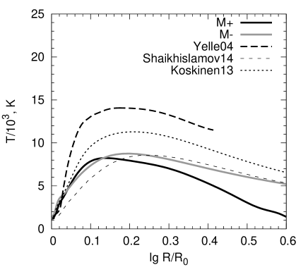
Figure 2: Height profiles of the temperature for the models M+, M-, Koskinen13, Shaikhislamov14, and Yelle04. Data for this and subsequent figures can be downloaded from %****␣paper1.tex␣Line␣350␣****https://github.com/Pantarktik/ARepIonovEtAl2017.

Figure 3: Height profiles of the velocity for models M+, M-, Koskinen13, Shaikhislamov14, and Yelle04.

We chose the following initial conditions for the computations. The atmosphere was taken to be isothermal at a temperature of 1300 K, which corresponds to the equilibrium temperature at a distance from the star equal to the semi-major axis of the orbit of HD 209458b. The density in the atmosphere was distributed according to a barometric law, and the gas velocity was initially equal to zero. The lower boundary of the computational domain was rigidly fixed at a distance equal to one planetary radius, with the conditions for reflection implemented. The upper boundary was not fixed; i.e. the atmosphere could both expand and contract during the simulations. The outer boundary condition was provided by the external pressure, which was taken to be equal to the gas pressure of the stellar wind at the corresponding orbital radius. Taking the stellar-wind parameters presented in Withbroe (1988), the external pressure is equal to $p_{ex}=1.6\times 10^{-6}$ dyne/cm². The atmosphere initially consisted of molecular hydrogen and helium, with a particle number fraction of helium equal to 0.15. One of the input parameters of the model is the total mass of the atmosphere. This was chosen empirically, such that the part of the atmosphere heated by XUV radiation fell into the computational domain. In our case, the mass of the atmosphere was $1\cdot 10^{18}$ g. The number density at the lower boundary was initially $7\times 10^{11}$ cm^-3. The spectrum of the star in the UV was taken to be the same as the spectrum of the current Sun, taken from Huebner, Keady & Lyon (1992) and recalculated for a distance of 0.045 AU. The computations were carried out until a steady state was reached.

Further, we compare the results for the model taking into account reactions involving suprathermal electrons (M+) and the model without these reactions (M-), that is, with an enhanced heating intensity. We also used the results obtained Yelle (2004) (Yelle04), Koskinen et al. (2012) (Koskinen13), and Shaikhislamov et al. (2014) (Shaikhislamov14) in this comparison.

3 Results

Figure 4: Height profiles of the density for models M+, M-, Koskinen13, Shaikhislamov14, and Yelle04.

Figures 2–4 show the computed height profiles of the temperature, velocity, and density for all the models considered. Since including suprathermal particles in the computations leads to a decrease in the heating intensity, we expect that including such particles should result in an appreciable decrease in the temperature of the atmosphere, as well as a reduction of the gas velocity, since the gas velocity is increased by heating.

We can see that our computations gave results that are qualitatively similar to the results of other studies. The height profiles of the temperature for models M+ and M-, as well as for models from other studies, are shown in Fig. 2. In agreement with expectations, taking into account photoelectrons leads to a reduction in the temperature of the atmosphere, with the difference between our two models growing with increasing radius. While the maximum temperature in model M- is roughly 9000 K, including suprathermal particles in the model reduces this, maximum temperature to 6000 K. Among the three models with which we compared our own computations, the best agreement is observed for the model Skaihislamov14. The temperatures in the Yelle04 and Koskinen13 models are several thousand Kelvin higher. However, the maximum temperature is located at roughly the same distance from the center in all the models: 1.3–1.5 $R_{0}$.

The velocity profiles shown in Fig. 3 are also qualitatively similar to the profiles obtained in other studies, and encompass the same range of velocities. Only at high heights do the models Koskinen13 and Skaihislamov14 display velocities exceeding the results of our model M-. The difference between models M+ and M- is especially large for the velocity: the gas velocity in the model without photoelectrons is a factor of a few higher.

Fig. 4 compares the density profiles for models M+, M-, Koskinen13, Shaikhislamov14, and Yelle04. Taking into account photoelectrons does not strongly influence the density profile, and the curves for models M+, M-, and Yelle04 virtually coincide.

The mass loss rate of the atmosphere can be estimated from the density and velocity at a given radius using the formula

$$\dot{M}=4\pi\rho(R)\upsilon(R)R^{2}$$ (5)

The computed mass loss rate does not change at heights above 1.2 planetary radii. The mass loss rate in model M- is $\dot{M}\approx 4\cdot 10^{10}$ g/s. The mass loss rate at the same heights in model M+ is $\dot{M}\approx 8\cdot 10^{9}$ g/s. The mass loss rate in model M- agrees with the results for the model Shaikhislamov14 ($7\cdot 10^{10}$ g/s) and essentially coincides with the model Koskinen13 ($4\cdot 10^{10}$ g/s). Taking into account the photoelectrons leads to a reduction in the mass loss rate by a factor of a few.

As was shown in Bisikalo et al. (2013a, b); Cherenkov, Bisikalo & Kaigorodov (2014), the regime and mass loss rate of the atmosphere are determined not only by the state of the atmosphere, but also by the parameters of the stellar wind. Therefore, the derived parameters of the atmosphere can be used as boundary conditions for three-dimensional gas-dynamical computations modeling the interaction between the planetary atmosphere and the stellar wind.

4 Conclusion

We have carried out simulations of the upper atmosphere of the exoplanet HD 209458b both including and excluding reactions involving suprathermal electrons. Including suprathermal particles leads to a strong reduction in the gas velocity. The mass loss rate falls by a factor of five in the computations with photoelectrons. Thus, we have demonstrated that suprathermal particles are an important factor in exoplanetary atmospheric processes, and neglecting them will lead to substantial errors in estimates of the parameters of the atmosphere.

5 Acknowledgements

This work was supported by the Russian Science Foundation (D.I. by Project 14-12-01048 and V.S. by Project 15-12-30038) and a grant of the President of the Russian Federation for the Support of Scientific Schools of the Russian Federation (project NSh-9576.2016.2).

References

- Bisikalo et al. (2013a) Bisikalo D., Kaygorodov P., Ionov D., Shematovich V., Lammer H., Fossati L., 2013a, Astrophys. J., 764, 19
- Bisikalo et al. (2013b) Bisikalo D. V., Kaigorodov P. V., Ionov D. E., Shematovich V. I., 2013b, Astronomy Reports, 57, 715
- Cherenkov, Bisikalo & Kaigorodov (2014) Cherenkov A. A., Bisikalo D. V., Kaigorodov P. V., 2014, Astronomy Reports, 58, 679
- Ehrenreich et al. (2015) Ehrenreich D. et al., 2015, Nature, 522, 459
- Fossati et al. (2010a) Fossati L. et al., 2010a, Astrophys. J., 720, 872
- Fossati et al. (2010b) Fossati L. et al., 2010b, Astrophys. J. (Letters), 714, L222
- García Muñoz (2007) García Muñoz A., 2007, Planet. Space Sci., 55, 1426
- Garvey & Green (1976) Garvey R. H., Green A. E. S., 1976, Phys. Rev. A, 14, 946
- Garvey, Porter & Green (1977) Garvey R. H., Porter H. S., Green A. E. S., 1977, Journal of Applied Physics, 48, 4353
- Huebner, Keady & Lyon (1992) Huebner W. F., Keady J. J., Lyon S. P., 1992, Astrophys. and Space Sci., 195, 1
- Ionov & Shematovich (2015) Ionov D. E., Shematovich V. I., 2015, Solar System Research, 49, 339
- Jackman, Garvey & Green (1977) Jackman C. H., Garvey R. H., Green A. E. S., 1977, J. Geophys. Res., 82, 5081
- Koskinen et al. (2012) Koskinen T. T., Harris M. J., Yelle R. V., Lavvas P., 2012, ArXiv e-prints
- Lammer et al. (2009) Lammer H. et al., 2009, Astron. and Astrophys., 506, 399
- Lammer et al. (2003) Lammer H., Selsis F., Ribas I., Guinan E. F., Bauer S. J., Weiss W. W., 2003, Astrophys. J. (Letters), 598, L121
- Lecavelier Des Etangs et al. (2010) Lecavelier Des Etangs A. et al., 2010, Astron. and Astrophys., 514, A72
- Linsky et al. (2010) Linsky J. L., Yang H., France K., Froning C. S., Green J. C., Stocke J. T., Osterman S. N., 2010, Astrophys. J., 717, 1291
- Marov, Shematovich & Bisicalo (1996) Marov M. Y., Shematovich V. I., Bisicalo D. V., 1996, Space Sci. Rev., 76, 1
- Murray-Clay, Chiang & Murray (2009) Murray-Clay R. A., Chiang E. I., Murray N., 2009, Astrophys. J., 693, 23
- Neale, Miller & Tennyson (1996) Neale L., Miller S., Tennyson J., 1996, Astrophys. J., 464, 516
- Pavlyuchenkov et al. (2015) Pavlyuchenkov Y. N., Zhilkin A. G., Vorobyov E. I., Fateeva A. M., 2015, Astronomy Reports, 59, 133
- Samarsky & Popov (1992) Samarsky A. A., Popov Y. P., 1992, Finite-difference methods of solving gas dynamic problems. - Moscow, Science
- Schneider (2016) Schneider J., 2016, The extrasolar planets encyclopaedia http://exoplanet.eu
- Seager (2010) Seager S., 2010, Exoplanet Atmospheres: Physical Processes
- Shaikhislamov et al. (2014) Shaikhislamov I. F., Khodachenko M. L., Sasunov Y. L., Lammer H., Kislyakova K. G., Erkaev N. V., 2014, Astrophys. J., 795, 132
- Shematovich (2008) Shematovich V. I., 2008, in American Institute of Physics Conference Series, Vol. 1084, American Institute of Physics Conference Series, Abe T., ed., pp. 1047–1054
- Shematovich (2010) Shematovich V. I., 2010, Solar System Research, 44, 96
- Shematovich, Bisikalo & Ionov (2015) Shematovich V. I., Bisikalo D. V., Ionov D. E., 2015, in Astrophysics and Space Science Library, Vol. 411, Characterizing Stellar and Exoplanetary Environments, Lammer H., Khodachenko M., eds., p. 105
- Shematovich, Ionov & Lammer (2014) Shematovich V. I., Ionov D. E., Lammer H., 2014, Astron. and Astrophys., 571, A94
- Tian et al. (2005) Tian F., Toon O. B., Pavlov A. A., De Sterck H., 2005, Astrophys. J., 621, 1049
- Vidal-Madjar et al. (2004) Vidal-Madjar A. et al., 2004, Astrophys. J. (Letters), 604, L69
- Vidal-Madjar et al. (2003) Vidal-Madjar A., Lecavelier des Etangs A., Désert J.-M., Ballester G. E., Ferlet R., Hébrard G., Mayor M., 2003, Nature, 422, 143
- Withbroe (1988) Withbroe G. L., 1988, Astrophys. J., 325, 442
- Yelle (2004) Yelle R. V., 2004, Icarus, 170, 167