Macquarie University at BioASQ 5b – Query-based Summarisation Techniques for Selecting the Ideal Answers

Abstract

Macquarie University’s contribution to the BioASQ challenge (Task 5b Phase B) focused on the use of query-based extractive summarisation techniques for the generation of the ideal answers. Four runs were submitted, with approaches ranging from a trivial system that selected the first $n$ snippets, to the use of deep learning approaches under a regression framework. Our experiments and the ROUGE results of the five test batches of BioASQ indicate surprisingly good results for the trivial approach. Overall, most of our runs on the first three test batches achieved the best ROUGE-SU4 results in the challenge.

1 Introduction

The main goal of query-focused multi-document summarisation is to summarise a collection of documents from the point of view of a particular query. In this paper we compare the use of various techniques for query-focused summarisation within the context of the BioASQ challenge. The BioASQ challenge Tsatsaronis et al. (2015) started in 2013 and it comprises various tasks centred on biomedical semantic indexing and question answering. The fifth run of the BioASQ challenge Nentidis et al. (2017), in particular, had three tasks:

• BioASQ 5a: Large-scale online biomedical semantic indexing.

• BioASQ 5b: Biomedical semantic question answering. This task had two phases:

  • Phase A: Identification of relevant information.

  • Phase B: Question answering.

• BioASQ 5c: Funding information extraction from biomedical literature.

The questions used in BioASQ 5b were of three types: yes/no, factoid, list, and summary. Submissions to the challenge needed to provide an exact answer and an ideal answer. Figure 1 shows examples of exact and ideal answers for each type of question.

yes/no

Does Apolipoprotein E (ApoE) have anti-inflammatory activity?

• Exact answer: yes

• Ideal answer: Yes. ApoE has anti-inflammatory activity

factoid

Which type of lung cancer is afatinib used for?

• Exact answer: EGFR-mutant non small cell lung carcinoma

• Ideal answer: Afatinib is a small molecule covalently binding and inhibiting the EGFR, HER2 and HER4 receptor tyrosine kinases. Trials showed promising efficacy in patients with EGFR-mutant NSCLC or enriched for clinical benefit from EGFR tyrosine kinase inhibitors gefitinib or erlotinib.

list

Which are the Yamanaka factors?

• Exact answer: [OCT4, SOX2, MYC, KLF4]

• Ideal answer: The Yamanaka factors are the OCT4, SOX2, MYC, and KLF4 transcription factors

summary

What is the role of brain natriuretic peptide in traumatic brain injury patients ?

• Exact answer: N/A

• Ideal answer: Brain natriuretic peptide concentrations are elevated in patients with traumatic brain during the acute phase and correlate with poor outcomes. In traumatic brain injury patients higher brain natriuretic peptide concentrations are associated with more extensive SAH, elevated ICP and hyponatremia. Brain natriuretic peptide may play an adaptive role in recovery through augmentation of cerebral blood flow.

Figure 1: Examples of questions with their exact and ideal answers in BioASQ 5b.

We can see that the ideal answers are full sentences that expand the information provided by the exact answers. These ideal answers could be seen as the result of query-focused multi-document summarisation. We therefore focused on Task 5b Phase B, and in that phase we did not attempt to provide exact answers. Instead, our runs provided the ideal answers only.

In this paper we will describe the techniques and experiment results that were most relevant to our final system runs. Some of our runs were very simple, yet our preliminary experiments revealed that they were very effective and, as expected, the simpler approaches were much faster than the more complex approaches.

Each of the questions in the BioASQ test sets contained the text of the question, the question type, a list of source documents, and a list of relevant snippets from the source documents. We used this information, plus the source documents which are PubMed abstracts accessible using the URL provided in the test sets.

Overall, the summarisation process of our runs consisted of the following two steps:

1. Split the input text (source documents or snippets) into candidate sentences and score each candidate sentence.

2. Return the $n$ sentences with highest score.

The value of $n$ was determined empirically and it depended on the question type, as shown in Table 1.

	Summary	Factoid	Yesno	List
n	6	2	2	3

Table 1: Value of $n$ (the number of sentences returned as the ideal answer) for each question type.

2 Simple Runs

As a first baseline, we submitted a run labelled trivial that simply returned the first $n$ snippets of each question. The reason for this choice was that, in some of our initial experiments, we incorporated the position of the snippet as a feature for a machine learning system. In those experiments, the resulting system did not learn anything and simply returned the input snippets verbatim. Subsequent experiments revealed that a trivial baseline that returned the first snippets of the question was very hard to beat. In fact, for the task of summarisation of other domains such as news, it has been observed that a baseline that returns the first sentences often outperformed other methods Brandow et al. (1995).

As a second baseline, we submitted a run labelled simple that selected the $n$ snippets what were most similar to the question. We used cosine similarity, and we tried two alternatives for computing the question and snippet vectors:

tfidf-svd:

First, generate the $tf.idf$ vector of the question and the snippets. We followed the usual procedure, and the $tf.idf$ vectors of these sentences are bag-of-word vectors where each dimension represents the $tf.idf$ of a word. Then, reduce the dimensionality of the vectors by selecting the first 200 components after applying Singular Value Decomposition. In contrast with a traditional approach to generate the $tf.idf$ (and SVD) vectors where the statistics are based on the input text solely (question and snippets in our case), we used the text of the question and the text of the ideal answers of the training data. The reason for using this variant was based on empirical results during our preliminary experiments.

word2vec:

Train Word2Vec Mikolov et al. (2013) using a set of over 10 million PubMed abstracts provided by the organisers of BioASQ. Using these pre-trained word embeddings, look up the word embeddings of each word in the question and the snippet. The vector representing a question (or snippet) is the sum of embeddings of each word in the question (or snippet). The dimension of the word embeddings was set to 200.

Table 2 shows the F1 values of ROUGE-SU4 of the resulting summaries. The table shows the mean and the standard deviation of the evaluation results after splitting the training data set for BioASQ 5b into 10 folds (for comparison with the approaches presented in the following sections).

	trivial	simple
		tfidf-svd	word2vec
Mean F1	0.2157	0.1643	0.1715
Stdev F1	0.0209	0.0097	0.0128

Table 2: ROUGE-SU4 of the simple runs.

We observe that the trivial run has the best results, and that the run that uses word2vec is second best. Our run labelled “simple” therefore used cosine similarity of the sum of word embeddings returned by word2vec.

3 Regression Approaches

For our run labelled regression, we experimented with the use of Support Vector Regression (SVR). The regression setup and features are based on the work by Malakasiotis et al. (2015), who reported the best results in BioASQ 3b (2015).

The target scores used to train the SVR system were the F1 ROUGE-SU4 score of each individual candidate sentence.

In contrast with the simple approaches described in Section 2, which used the snippets as the input data, this time we used all the sentences of the source abstracts. We also incorporated information about whether the sentence was in fact a snippet as described below.

As features, we used:

• $tf.idf$ vector of the candidate sentence. In contrast with the approach described in Section 2, The statistics used to determine the $tf.idf$ vectors were based on the text of the question, the text of the ideal answers, and the text of the snippets.

• Cosine similarity between the $tf.idf$ vector of the question and the $tf.idf$ vector of the candidate sentence.

• The smallest cosine similarity between the $tf.idf$ vector of candidate sentence and the $tf.idf$ vector of each of the snippets related to the question. Note that this feature was not used by Malakasiotis et al. (2015).

• Cosine similarity between the sum of word2vec embeddings of the words in the question and the word2vec embeddings of the words in the candidate sentence. As in our run labelled “simple”, we used vectors of dimension 200.

• Pairwise cosine similarities between the words of the question and the words of the candidate sentence. As in the work by Malakasiotis et al. (2015), we used word2vec to compute the word vectors. These word vectors were the same as used in Section 2. We then computed the pairwise cosine similarities and selected the following features:

  • The mean, median, maximum, and minimum of all pairwise cosine similarities.

  • The mean of the 2 highest, mean of the 3 highest, mean of the 2 lowest, and mean of the 3 lowest.

• Weighted pairwise cosine similarities, also based in the work by Malakasiotis et al. (2015). In particular, now each word vector was multiplied by the $tf.idf$ of the word, we computed the pairwise cosine similarities, and we used the mean, median, maximum, minimum, mean of 2 highest, mean of 3 highest, mean of 2 lowest, and mean of 3 lowest.

Figure 2 shows the result of grid search by varying the $gamma$ parameter of SVR, fixing $C$ to 1.0, and using the $RBF$ kernel. The figure shows the result of an extrinsic evaluation that reports the F1 ROUGE-SU4 of the final summary, and the result of an intrinsic evaluation that reports the Mean Square Error (MSE) between the target and the predicted SU4 of each individual candidate sentence.

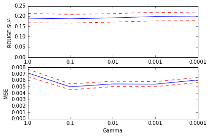
Figure 2: Grid search of the Gamma parameter for the experiments using Support Vector Regression. The continuous lines indicate the mean of 10-fold cross-validation over the training data set of BioASQ 5b. The dashed lines indicate 2 $\times$ the standard deviation.

We can observe discrepancy between the results of the intrinsic and the extrinsic evaluations. This discrepancy could be due to the fact that the data are highly imbalanced in the sense that most annotated SU4 scores in the training data have low values. Consequently, the regressor would attempt to minimise the errors in the low values of the training data at the expense of errors in the high values. But the few sentences with high SU4 scores are most important for the final summary, and these have higher prediction error. This can be observed in the scatter plot of Figure 3, which plots the target against the predicted SU4 in the SVR experiments for each value of $gamma$. The SVR system has learnt to predict the low SU4 scores to some degree, but it does not appear to have learnt to discriminate among SU4 scores over a value of 0.4.

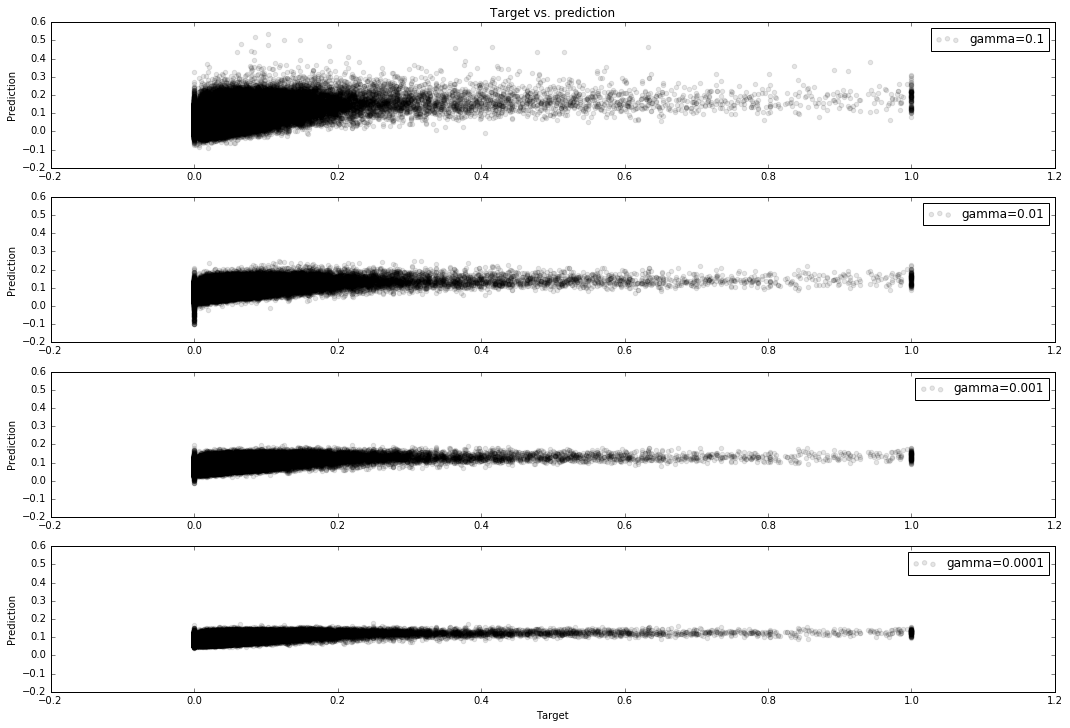
Figure 3: Target vs. predicted SU4 in the SVR experiments for various values of $gamma$.

Our run labelled “regression” used $gamma=0.1$ since it gave the best MSE in our intrinsic evaluation, and Figure 3 appeared to indicate that the system learnt best.

4 Deep Learning Approaches

For our run labelled nnr we experimented with the use of deep learning approaches to predict the candidate sentence scores under a regression setup. The regression setup is the same as in Section 3.

Figure 4 shows the general architecture of the deep learning systems explored in our experiments.

Figure 4: Architecture of the regression system.

In a pre-processing stage, and not shown in the figure, the main text of the source PubMed abstracts is split into sentences by using the default NLTK sentence segmenter. The candidate sentences and questions undergo a simple preprocessing stage that removes punctuation characters, and lowercases the string and splits on blank spaces. Then, these are fed to the system as a sequence of token identifiers. Figure 4 shows that the input to the system is a candidate sentence and the question (as sequences of token IDs). The input is first converted to sequences of word embeddings by applying an embedding matrix. The word embedding stage is followed by a sentence and question reduction stage that combines the word embeddings of each sentence into a sentence embedding. Then, the sentence embedding and the question embedding are compared by applying a similarity operation, and the vector resulting from the comparison is concatenated to the sentence embedding for a final regression comprising of a hidden layer of rectilinear units (relu) and a final linear combination.

The weights of all stages are optimised by backpropagation in order to minimise the MSE of the predicted score at training time. Our experiments varied on the approach for sentence and question reduction, and the approach to incorporate the similarity between sentence and question, as described below.

To produce word embeddings we use word2vec, trained on a collection of over 10 million PubMed abstracts as described in previous sections. The resulting word embeddings are encoded in the embedding matrix of Figure 4. We experimented with the possibility of adjusting the weights of the embedding matrix by backpropagation, but the results did not improve. The results reported in this paper, therefore, used a constant embedding matrix. We experimented with various sizes of word embeddings and chose 100 for the experiments in this paper.

After obtaining the word embeddings, we experimented with the following approaches to produce the sentence vectors:

Mean:

The word embeddings provided by word2vec map words into a dimensional space that roughly represents the word meanings, such that words that are similar in meaning are also near in the embedded space. This embedding space has the property that some semantic relations between words are also mapped in the embedded space Mikolov et al. (2013). It is therefore natural to apply vector arithmetics such as the sum or the mean of word embeddings of a sentence in order to obtain the sentence embedding. In fact, this approach has been used in a range of applications, on its own, or as a baseline against which to compare other more sophisticated approaches to obtain word embeddings, e.g. work by Yu et al. (2014) and Kageback et al. (2014). To accommodate for different sentence lengths, in our experiments we use the mean of word embeddings instead of the sum.

CNN:

Convolutional Neural Nets (CNN) were originally developed for image processing, for tasks where the important information may appear on arbitrary fragments of the image Fukushima (1980). By applying a convolutional layer, the image is scanned for salient information. When the convolutional layer is followed by a maxpool layer, the most salient information is kept for further processing.

We follow the usual approach for the application of CNN for word sequences, e.g. as described by Kim (2014). In particular, the embeddings of the words in a sentence (or question) are arranged in a matrix where each row represents a word embedding. Then, a set of convolutional filters are applied. Each convolutional filter uses a window of width the total number of columns (that is, the entire word embedding). Each convolutional filter has a fixed height, ranging from 2 to 4 rows in our experiments. These filters aim to capture salient ngrams. The convolutional filters are then followed by a maxpool layer.

Our final sentence embedding concatenates the output of 32 different convolutional filters, each at filter heights 2, 3, and 4. The sentence embedding, therefore, has a size of $32\times 3=96$.

LSTM:

The third approach that we have used to obtain the sentence embeddings is recurrent networks, and in particular Long Short Term Memory (LSTM). LSTM has been applied successfully to applications that process sequences of samples Hochreiter et al. (1997). Our experiments use TensorFlow’s implementation of LSTM cells as described by Pham et al. (2013).

In order to incorporate the context on the left and right of each word we have used the bidirectional variant that concatenates the output of a forward and a backward LSTM chain. As is usual practice, all the LSTM cells in the forward chain share a set of weights, and all the LSTM cells in the backward chain share a different set of weights. This way the network can generalise to an arbitrary position of a word in the sentence. However, we expect that the words of the question behave differently from the words of the candidate sentence. He have therefore used four distinct sets of weights, two for the forward and backward chains of the candidate sentences, and two for the question sentences.

In our experiments, the size of the output of a chain of LSTM cells is the same as the number of features in the input data, that is, the size of the word embeddings. Accounting for forward and backward chains, and given word embeddings of size 100, the size of the final sentence embedding is 200.

Figure 4 shows how we incorporated the similarity between the question and the candidate sentence. In particular, we calculated a weighted dot product, where the weights $w_{i}$ can be learnt by backpropagation:

$$sim(q,s)=\sum_{i}w_{i}q_{i}s_{i}$$

Since the sum will be performed by the subsequent relu layer, our comparison between the sentence and the question is implemented as a simple element-wise product between the weights, sentence embeddings, and question embeddings.

An alternative similarity metric that we have also tried is as proposed by Yu et al. (2014). Their similarity metric allows for interactions between different components of the sentence vectors, by applying a $d\times d$ weight matrix $W$, where $d$ is the sentence embedding size, and adding a bias term:

$$simYu(q,s)=q^{T}Ws+b$$

In both cases, the optimal weights and bias are learnt by backpropagation as part of the complete neural network model of the system.

Table 3 shows the average MSE of 10-fold cross-validation over the training data of BioASQ 5b.

Method	Plain	Sim	SimYu
Tf.idf	0.00354
SVD	0.00345	0.00334	0.00342
Mean	0.00341	0.00330	0.00331
CNN	0.00350	0.00348	0.00349
LSTM	0.00344	0.00335	0.00336

Table 3: Average MSE of 10-fold cross-validation.

“Tf.idf” is a neural network with a hidden layer of 50 relu cells, followed by a linear cell, where the inputs are the tf.idf of the words. “SVD” computes the sentence vectors as described in Section 2, with the only difference being that now we chose 100 SVD components (instead of 200) for comparison with the other approaches shown in Table 3.

We observe that all experiments perform better than the Tf.idf baseline, but there are no major differences between the use of SVD and the three approaches based on word embeddings. The systems which integrated a sentence similarity performed better than those not using it, though the differences when using CNN are negligible. Each cell in Table 3 shows the best results after grid searches varying the dropout rate and the number of epochs during training.

For the “nnr” run, we chose the combination “Mean” and “Sim” of Table 3, since they produced the best results in our experiments (although only marginally better than some of the other approaches shown in the table).

5 Submission Results

At the time of writing, the human evaluations had not been released, and only the ROUGE results of all 5 batches were available. Table 4 shows the F1 score of ROUGE-SU4.

System	Batch 1	Batch 2	Batch 3	Batch 4	Batch 5
trivial	0.5498	0.4901	0.5832	0.5431	0.4950
simple	0.5068	0.5182	0.6186	0.5769	0.5840
regression	0.5186	0.4795	0.5785	0.5436	0.4784
nnr	0.4192	0.3920	0.5196	0.4445	0.4000

Table 4: ROUGE-SU4 of the 5 batches of BioASQ 2017.

Figure 5 shows the same information as a plot that includes our runs and all runs of other participating systems with higher ROUGE scores. The figure shows that, in the first three batches, only one run by another participant was among our results (shown as a dashed line in the figure). Batches 4 and 5 show consistent results by our runs, and improved results of runs of other entrants.

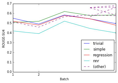
Figure 5: Top ROUGE-SU4 scores of the 5 batches of BioASQ 2017.

The results are consistent with our experiments, though the absolute values are higher than those in our experiments. This is probably because we used the entire training set of BioASQ 5b for our cross-validation results, and this data is the aggregation of the training sets of the BioASQ tasks of previous years. It is possible that the data of latter years are of higher quality, and it might be useful to devise learning approaches that would account for this possibility.

6 Conclusions

At the time of writing, only the ROUGE scores of BioASQ 5b were available. The conclusions presented here, therefore, do not incorporate any insights of the human judgements that are also part of the final evaluation of BioASQ.

Our experiments show that a trivial baseline system that returned the first $n$ snippets appears to be hard to beat. This implies that the order of the snippets matters. Even though the judges were not given specific instructions about the order of the snippets, it would be interesting to study what criteria they used to present the snippets.

Our runs using regression were not significantly better than simpler approaches, and the runs using deep learning reported the lowest results. Note, however, that the input features used in the runs using deep learning did not incorporate information about the snippets. Table 3 shows that the results using deep learning are comparable to results using tf.idf and using SVD, so it is possible that an extension of the system that incorporates information from the snippets would equal or better the other systems.

Note that none of the experiments described in this paper used information specific to the biomedical domain and therefore the methods described here could be applied to any other domain.

References

- Brandow et al. (1995) Ronald Brandow, Karl Mitze, and Lisa F. Rau. 1995. Automatic condensation of electronic publications by sentence selection. Information Processing and Management 31(5):675–685.
- Fukushima (1980) Kunihiko Fukushima. 1980. Neocognitron: A self-organizing neural network model for a mechanism of pattern recognition unaffected by shift in position. Biological Cybernetics 36(4):193–202.
- Hochreiter et al. (1997) Sepp Hochreiter, Jürgen Schmidhuber, Sepp Hochreiter, Jürgen Schmidhuber, and Jürgen Schmidhuber. 1997. Long short-term memory. Neural Computation 9(8):1735–80.
- Kageback et al. (2014) Mikael Kageback, Olof Mogren, Nina Tahmasebi, and Devdatt Dubhashi. 2014. Extractive summarization using continuous vector space models. In Proceedings of the 2nd Workshop on Continuous Vector Space Models and their Compositionality (CVSC). pages 31–39.
- Kim (2014) Yoon Kim. 2014. Convolutional neural networks for sentence classification. Proceedings of the 2014 Conference on Empirical Methods in Natural Language Processing (EMNLP 2014) pages 1746–1751.
- Malakasiotis et al. (2015) Prodromos Malakasiotis, Emmanouil Archontakis, and Ion Androutsopoulos. 2015. Biomedical question-focused multi-document summarization: ILSP and AUEB at BioASQ3. In CLEF 2015 Working Notes.
- Mikolov et al. (2013) Tomas Mikolov, Kai Chen, Greg Corrado, and Jeffrey Dean. 2013. Efficient estimation of word representations in vector space. In Proceedings of Workshop at ICLR. pages 1–12.
- Nentidis et al. (2017) Anastasios Nentidis, Konstantinos Bougiatiotis, Anastasia Krithara, Georgios Paliouras, and Ioannis Kakadiaris. 2017. Results of the fifth edition of the BioASQ Challenge. In Proceedings BioNLP 2017.
- Pham et al. (2013) Vu Pham, Théodore Bluche, Christopher Kermorvant, and Jérôme Louradour. 2013. Dropout improves recurrent neural networks for handwriting recognition. Technical report.
- Tsatsaronis et al. (2015) George Tsatsaronis, Georgios Balikas, Prodromos Malakasiotis, Ioannis Partalas, Matthias Zschunke, Michael R Alvers, Dirk Weissenborn, Anastasia Krithara, Sergios Petridis, Dimitris Polychronopoulos, Yannis Almirantis, John Pavlopoulos, Nicolas Baskiotis, Patrick Gallinari, Thierry Artiéres, Axel-Cyrille Ngonga Ngomo, Norman Heino, Eric Gaussier, Liliana Barrio-Alvers, Michael Schroeder, Ion Androutsopoulos, and Georgios Paliouras. 2015. An overview of the BIOASQ large-scale biomedical semantic indexing and question answering competition. BMC Bioinformatics 16(1):138.
- Yu et al. (2014) Lei Yu, Karl Moritz Hermann, Phil Blunsom, and Stephen Pulman. 2014. Deep learning for answer sentence selection. In NIPS Deep Learning Workshop. page 9.