On the geometry of folded cuspidal edges

Abstract

We study the geometry of cuspidal $S_{k}$ singularities in $\mathbb{R}^{3}$ obtained by folding generically a cuspidal edge. In particular we study the geometry of the cuspidal cross-cap $M$, i.e. the cuspidal $S_{0}$ singularity. We study geometrical invariants associated to $M$ and show that they determine it up to order 5. We then study the flat geometry (contact with planes) of a generic cuspidal cross-cap by classifying submersions which preserve it and relate the singularities of the resulting height functions with the geometric invariants.

1 Introduction

Given a parametrisation $\phi:U\subset\mathbb{R}^{2}\rightarrow\mathbb{R}^{3}$ of a surface $N$, where $U$ is an open set, we say that $N$ is a cuspidal $S_{k}$ singularity if it admits a parametrisation $\phi$ which is $\mathcal{A}$-equivalent (equivalent by diffeomorphisms in source and target) to $f(x,y)=(x,y^{2},x^{k+1}y^{3}+y^{5})$. In the particular case of $k=0$, the cuspidal $S_{0}$-singularity is the cuspidal cross-cap (or folded umbrella), which we denote by $M$. In this case, the image of $f$ resembles that of the Whitney umbrella but it contains a cuspidal edge transversal to the double point curve (see Figure 1). Cuspidal $S_{k}$ singularities are types of frontal singularities and the cuspidal cross-cap in particular naturally appears in different contexts of differential geometry. For example, it is a generic singularity of bicaustics, the surface drawn by the cuspidal edges of a 1-parameter family of caustics in 3-space [1]. It is also the singularity which appears in a developable surface of a space curve at a point of zero torsion [9]. It even appears as a type of generic singularity in dynamical systems related to relaxational equations ([11], [39]).

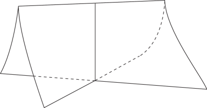
Figure 1: The standard cuspidal cross-cap.

There has been a recent impulse in the study of the differential geometry of singular surfaces. Defining new geometric invariants (namely, invariants of surfaces under the action of $SO(3)$ in $\mathbb{R}^{3}$) and applying singularity theory techniques has become a crucial subject to attain this goal. For instance, there have been many developments considering the geometry of the cross-cap (Whitney umbrella) ([4, 7, 12, 13, 14, 15, 16, 27, 28, 29]). Considering the most simple type of wave front singularity, the cuspidal edge, there have also been many significant advances ([21, 23, 24, 26, 30, 34, 37]). Many papers are devoted to the study of singularities of wave fronts or frontals in general ([25, 33, 35]). Also, in [22], the geometry of corank 1 surface singularities is studied in general.

In order to study the generic geometry of a certain singular surface it is convenient to have a normal form with arbitrary coefficients which give the necessary freedom to capture all the generic geometry. Such a normal form must be obtained by applying diffeomorphisms in the source, but only isometries in the target. In [38], a normal form was obtained for the cross-cap. In [23], Martins and the second author obtain a normal form for the cuspidal edge. In the case of the cross-cap the authors consider the normal form modulo order 3 terms, and in the cuspidal edge case the normal form is considered up to order 3 terms. However, for more degenerate singularities the order one must consider in order to capture interesting geometrical features can grow considerably. For example, taking a generic section of the cuspidal cross-cap $M$ through the origin yields a ramphoid (or (2,5)-)cusp, therefore, it is reasonable to think that a normal form must consider up to order 5 terms. We avoid this difficulty by taking an alternative approach: given a generic cuspidal edge, if we take a plane transversal to the cuspidal edge curve and fold the cuspidal edge along that plane we obtain a cuspidal cross-cap. This was first noticed by Arnol’d in [2, page 120] and generalized by the second author in [32]. If the order of contact of the cuspidal edge with the folding plane is $k+1$, the resulting surface has an $S_{k}$ singularity.

The idea of folding maps (more precisely, studying geometry by considering its symmetries) dates back to Klein’s Erlangen programme. In [8] Bruce and Wilkinson studied this phenomenon from the singularity theory point of view and it is starting to be of interest for geometers in singularity theory again ([3, 18]). More recently, Peñafort-Sanchis has studied (generalized) reflection maps as a source of corank 2 maps and has proved Lê’s conjecture about the injectivity of corank 2 maps for this class of maps ([31]). In our case, considering the cuspidal cross-cap obtained by folding a cuspidal edge is obviously more restrictive than studying a generic cuspidal cross-cap. We shall show that from the point of view of flat geometry, there is only one generic singularity of the height function which is not captured by this process. Namely, the reflecting plane is the tangent cone of the resulting cuspidal cross-cap and all of the surface is on one side of this plane, but generically the surface could be on both sides of the tangent cone, as we shall show. This suggests that the set of germs of surfaces with a cuspidal cross-cap obtained by folding a cuspidal edge has (in a certain sense) codimension 1 in the set of germs of surfaces with a cuspidal cross-cap singularity. However, there are more advantages than disadvantages (besides the fact of not needing a special normal form) since we can relate the geometry of the cuspidal cross-cap with that of the cuspidal edge it comes from. In fact, we find a relation between a generic singularity of a height function on a generic cuspidal cross-cap and the torsion of a certain curve in the cuspidal edge before folding it.

The paper is organized as follows: Section 2 explains the setting and studies geometric invariants of the cuspidal cross-cap, and cuspidal $S_{k}$ singularities obtained by folding a cuspidal edge. We consider geometric invariants of the cuspidal edge in the cuspidal cross-cap, the double point curve and of the ramphoid cusp obtained by a generic section through the origin. Some relations are given amongst these invariants and it is shown which of these invariants determine the cuspidal cross-cap up to order 5. Section 3 is devoted to the classification of submersions preserving $M$. The singularities of these submersions model the singularities of the height functions on $M$ and capture the geometry of the contact of $M$ with planes. These singularities are related to the geometric invariants considered in Section 2. We then study the duals of the different generic $M$. Finally, in Section 4, we consider the geometry of the tangent developable of a space curve at a point of zero torsion.

Acknowledgements: The authors would like to thank Farid Tari for helpful discussions and the referees for valuable suggestions which improved the scope and presentation of the results.

2 Geometrical invariants

2.1 Normal form of the cuspidal edge and its invariants

A map-germ $f:(\mathbb{R}^{2},0)\rightarrow(\mathbb{R}^{3},0)$ is a frontal if there exists a well defined normal unit vector field $\nu$ along $f$, namely, $|\nu|=1$ and for any $X\in T_{p}\mathbb{R}^{2}$, $df_{p}(X)\cdot\nu(p)=0$. A frontal $f$ with a unit normal unit vector field $\nu$ is a front if the pair $(f,\nu)$ is an immersion. Since at a cuspidal edge $f:(\mathbb{R}^{2},0)\rightarrow(\mathbb{R}^{3},0)$, there is always a well defined normal unit vector field $\nu$ along $f$, and the pair $(f,\nu)$ is an immersion, a cuspidal edge is a front. On the other hand, at a cuspidal cross-cap $f:(\mathbb{R}^{2},0)\rightarrow(\mathbb{R}^{3},0)$, there is always a well defined normal unit vector field $\nu$ along $f$, but the pair $(f,\nu)$ is not an immersion, a cuspidal cross-cap is a frontal but not a front. Let $f:(\mathbb{R}^{2},0)\rightarrow(\mathbb{R}^{3},0)$ be a frontal with a normal unit vector field $\nu$. Consider the function $\lambda=\det(f_{x},f_{y},\nu)$, where $(x,y)$ are the coordinates of $\mathbb{R}^{2}$. Then $S(f)=\{\lambda^{-1}(0)\}$, where $S(f)$ is the set of singular point of $f$. A singular point $q$ is non-degenerate if $d\lambda(q)\neq 0$. If $q$ is a non-degenerate singular point, there is a well defined vector field $\eta$ in $\mathbb{R}^{2}$, such that $df(\eta)=0$ on $S(f)$. Such a vector field is called a null vector field. A singular point $q$ is called of first kind if $\eta\lambda(q)\neq 0$. A singular point $q$ is of first kind of a front if $f$ is a cuspidal edge ([21]). Let $f:(\mathbb{R}^{2},0)\rightarrow(\mathbb{R}^{3},0)$ be a frontal with a normal unit vector field $\nu$, and $0$ a singular point of the first kind. Since $\eta$ is transversal to $S(f)$, we can consider another vector field $\xi$ which is tangent to $S(f)$ and such that $(\xi,\eta)$ is positively oriented. Such a pair of vector fields is called an adapted pair. An adapted coordinate system $(u,v)$ of $\mathbb{R}^{2}$ is a coordinate system such that $S(f)$ is the $u$-axis, $\partial_{v}$ is the null vector field and there are no singular points besides the $u$-axis. Let $\gamma$ be a parametrisation of the singular curve $S(f)$ and let $\widehat{\gamma}=f\circ\gamma$.

In [23] certain geometric invariants of cuspidal edges are studied. Amongst them are the singular curvature, the limiting normal curvature, the cuspidal curvature and the cusp-directional torsion ($\kappa_{s}$, $\kappa_{\nu}$, $\kappa_{c}$ and $\kappa_{t}$, resp.), and these are given as follows:

$$\kappa_{s}(t)=\displaystyle\operatorname{sgn}(d\lambda(\eta))\frac{\det(\widehat{\gamma}^{\prime}(t),\widehat{\gamma}^{\prime\prime}(t),\nu(\gamma(t)))}{|\widehat{\gamma}^{\prime}(t)|^{3}},\quad\kappa_{\nu}(t)=\displaystyle\frac{\langle\widehat{\gamma}^{\prime\prime}(t),\nu(\gamma(t))\rangle}{|\widehat{\gamma}^{\prime}(t)|^{2}},$$ (2.1)

and

$$\kappa_{c}(t) =\displaystyle\frac{|\xi f|^{3/2}\det(\xi f,\eta^{2}f,\eta^{3}f)}{|\xi f\times\eta^{2}f|^{5/2}}(\gamma(t)),$$ (2.2)

$$\kappa_{t}(t) =\displaystyle\frac{\det(\xi f,\eta^{2}f,\xi\eta^{2}f)}{|\xi f\times\eta^{2}f|^{2}}(\gamma(t))-\frac{\det(\xi f,\eta^{2}f,\xi\eta^{2}f)\langle\xi f,\eta^{2}f\rangle}{|\xi f|^{2}|\xi f\times\eta^{2}f|^{2}}(\gamma(t)),$$ (2.3)

where ^′ stands for the differential with respect to the considered variable, and $\zeta^{i}f$ stands for the $i$ times directional derivative of $f$ by the vector field $\zeta$. A detailed description and geometrical interpretation of $\kappa_{s}$ and $\kappa_{\nu}$ can be found in [34], of $\kappa_{c}$ in [25] and of $\kappa_{t}$ in [23]. Since $\xi f\times\eta^{2}f\neq 0$ for singularities of the first kind, these invariants can be also defined for the singularities of the first kind.

A normal form for a cuspidal edge is obtained in [23, Theorem 3.1]. The same proof works for the case of a singular point of the first kind, and we obtain:

Proposition 2.1.

Let $f:(\mathbb{R}^{2},0)\rightarrow(\mathbb{R}^{3},0)$ be a frontal with a normal unit vector field $\nu$. Let $0$ be a singular point of the first kind. Then there exist a coordinate system $(x,y)$ on $(\mathbb{R}^{2},0)$ and an isometry-germ $\Phi:(\mathbb{R}^{3},0)\to(\mathbb{R}^{3},0)$ such that

$$\Phi\circ f(x,y)=\left(x,a(x)+\dfrac{y^{2}}{2},b_{0}(x)+b_{1}(x)y^{2}+b_{2}(x)y^{3}+b_{3}(x,y)y^{4}\right),$$ (2.4)

where $a,b_{0},b_{1},b_{2},b_{3}$ be smooth functions such that $a(0)=a^{\prime}(0)=b_{0}(0)=b_{0}^{\prime}(0)=b_{1}(0)=0.$

Let $f$ be a map-germ given by (2.4). If $b_{2}(0)\neq 0$, then $f$ is a cuspidal edge, and if $b_{2}(0)=0$, $b_{2}^{\prime}(0)\neq 0$, then $f$ is a cuspidal cross-cap. Moreover, if $b_{2}^{(i)}(0)=0$ $(i=1,\ldots,k)$ and $b_{2}^{(k+1)}(0)\neq 0$, then $f$ is $\mathcal{A}$-equivalent to $(x,y^{2},x^{k+1}y^{3}\pm y^{5})$ (i.e. a cuspidal $S_{k}^{\pm}$ singularity, and a cuspidal $S_{0}$ singularity is a cuspidal cross-cap). Furthermore, we have:

$$|\kappa_{s}(0)|=|a^{\prime\prime}(0)|,\quad\kappa_{\nu}(0)=b_{0}^{\prime\prime}(0),\quad\kappa_{c}(0)=6b_{2}(0),\quad\kappa_{t}(0)=2b_{1}^{\prime}(0).$$

If $b_{2}(0)=0$, (namely, non-cuspidal edge), one can define other invariants. Let $f$ be a map-germ given by (2.4) with $b_{2}(0)=0$. Then one can take a null vector satisfying $\xi f\cdot\tilde{\eta}^{2}f(0)=\xi f\cdot\tilde{\eta}^{3}f(0)=0.$ Then there exist $l$ such that $\tilde{\eta}^{3}f(0)=l\tilde{\eta}^{2}f(0)$. Following [17], we define two real numbers by

$$B= \dfrac{|\xi f|^{2}\det\Big{(}\xi f,\ \tilde{\eta}^{2}f,\ \tilde{\eta}^{4}f\Big{)}}{|\xi f\times\tilde{\eta}^{2}f|^{3}}\Bigg{|}_{(u,v)=0},$$ (2.5)

$$\kappa_{c}^{{\rm r}}= \dfrac{|\xi f|^{5/2}\det\Big{(}\xi f,\ \tilde{\eta}^{2}f,\ 3\tilde{\eta}^{5}f-10\,l\,\tilde{\eta}^{4}f\Big{)}}{|\xi f\times\tilde{\eta}^{2}f|^{7/2}}\Bigg{|}_{(u,v)=0}.$$ (2.6)

$B$ and $\kappa_{c}^{{\rm r}}$ do not depend on the choice of $(\xi,\tilde{\eta})$. The invariant $B$ measures the bias of a curve around the singular point and it is called bias, and $\kappa_{c}^{{\rm r}}$ measures wideness of the cusp and it is called secondary cuspidal curvature. See [17] for details.

2.2 Invariants of singular space curve

In order to study special curves on the cuspidal $S_{k}^{\pm}$ singularities, we consider geometric invariants of singular space curves. Let $\gamma:(\mathbb{R},0)\to(\mathbb{R}^{3},0)$ be a curve and assume that $\gamma^{\prime}(0)=(0,0,0)$. The point $0$ is called an $A$-type point if $\gamma^{\prime\prime}(0)\neq(0,0,0)$, and $0$ is called $(2,3)$-type if $\gamma^{\prime\prime}(0)\times\gamma^{\prime\prime\prime}(0)\neq(0,0,0)$.

Let $0$ be an $A$-type singular point of $\gamma$, then, following [24], we define

$$\kappa_{sing}(\gamma)=\dfrac{|\gamma^{\prime\prime}(0)\times\gamma^{\prime\prime\prime}(0)|}{|\gamma^{\prime\prime}(0)|^{5/2}}.$$

Moreover, let $0$ be a $(2,3)$-type singular point of $\gamma$, then we define

$$\tau_{sing}(\gamma)=\dfrac{\sqrt{|\gamma^{\prime\prime}(0)|}\det(\gamma^{\prime\prime}(0),\gamma^{\prime\prime\prime}(0),\gamma^{(4)}(0))}{|\gamma^{\prime\prime}(0)\times\gamma^{\prime\prime\prime}(0)|^{2}},$$

where $f^{(i)}$ stands for the $i$-th derivative of $f$ with respect to the considered variable. We set

$$\sigma_{sing}(\gamma)=\dfrac{\left(\langle\gamma^{\prime\prime}(0)\times\gamma^{\prime\prime\prime}(0),\gamma^{\prime\prime}(0)\times\gamma^{(4)}(0)\rangle-2\dfrac{|\gamma^{\prime\prime}(0)\times\gamma^{\prime\prime\prime}(0)|^{2}\langle\gamma^{\prime\prime}(0),\gamma^{\prime\prime\prime}(0)\rangle}{\langle\gamma^{\prime\prime}(0),\gamma^{\prime\prime}(0)\rangle}\right)}{\langle\gamma^{\prime\prime}(0),\gamma^{\prime\prime}(0)\rangle^{11/4}}.$$

If two curves $\gamma_{1},\gamma_{2}:(\mathbb{R},0)\to(\mathbb{R}^{3},0)$ satisfy $\kappa_{sing}(\gamma_{1})=\kappa_{sing}(\gamma_{2})$, $\tau_{sing}(\gamma_{1})=\tau_{sing}(\gamma_{2})$ and $\sigma_{sing}(\gamma_{1})=\sigma_{sing}(\gamma_{2})$, then there exists an isometry and parameters $t_{1}$, $t_{2}$ such that $j^{3}\gamma_{1}(0)=j^{3}\gamma_{2}(0)$ with respect to the parameters $t_{1}$, $t_{2}$. Thus the invariants $\{\kappa_{sing}(\gamma),\sigma_{sing}(\gamma),\tau_{sing}(\gamma)\}$ can be used as invariants for $(2,3)$-type singular space curves up to fourth degree. See [24] for details.

2.3 Folded cuspidal edge

Let $f:(\mathbb{R}^{2},0)\to(\mathbb{R}^{3},0)$ be the map-germ defined by the right-hand side of (2.4). Let $(X,Y,Z)$ denote the coordinate system on $(\mathbb{R}^{3},0)$. We now consider the fold map whose singular set is the reflecting hyperplane $Z=0$, given by

$$g(X,Y,Z)=(X,Y,Z^{2})$$

and consider the cuspidal edge folded along the plane $Z=0$, i.e., the composition

$$\phi=g\circ f$$ (2.7)

of the parametrisation of the cuspidal edge with the fold map. We may assume that $a(0)=a^{\prime}(0)=b_{0}(0)=0,\ b_{2}(0)\neq 0$ without loss of generality. In order for $\phi=g\circ f$ to be a cuspidal $S_{k}$ singularity, we need the condition

$$b_{0}(0)=\cdots=b_{0}^{(k)}(0)=0,b_{0}^{(k+1)}(0)\neq 0,$$

(see [32, Theorem 3.2]) which is equivalent to the cuspidal edge curve having a $(k+1)$th degree contact with the plane $Z=0$ (see Figure 2). By Shafarevich [36], if ${\mathcal{X}}$ is an irreducible affine variety in $\mathbb{R}^{n}$ defined by the ideal $I$ then the equations for the tangent cone of ${\mathcal{X}}$ are the lowest degree terms of the polynomials in $I$. Therefore, the tangent cone of the cuspidal $S_{k}$ singularity is the plane $Z=0$.

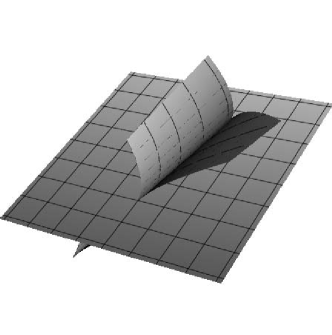
$\longrightarrow$      

Figure 2: A cuspidal cross-cap obtained by folding a cuspidal edge.

We now compute the geometric invariants of $\phi$. Since $\phi$ is a cuspidal $S_{k}$ singularity, in particular, a singularity of the first kind, we have the invariants (2.1), (2.2) and (2.3). The singular set of $\phi$ is given by $S(\phi)=\{y=0\}$. We set $\Sigma=\phi(S(\phi))$. Then $\Sigma$ is the image of $\phi(x,0)=(x,a(x),b_{0}(x)^{2})$. The osculating plane of $\Sigma$ at the origin is the plane orthogonal to the vector $(0,-2b_{0}^{\prime}(0)^{2},a^{\prime\prime}(0))$.

Proposition 2.2.

For a cuspidal $S_{k}$ singularity $\phi$ obtained by (2.7), we have

$$\kappa_{s}^{\phi}(0) =a^{\prime\prime}(0),$$

$$(\kappa_{s}^{\phi})^{\prime}(0) =8b_{1}(0)b_{0}^{\prime}(0)^{3}+a^{\prime\prime\prime}(0),$$

$$(\kappa_{s}^{\phi})^{\prime\prime}(0) =16b_{0}^{\prime}(0)^{3}b_{1}^{\prime}(0)-16b_{0}^{\prime}(0)^{4}a^{\prime\prime}(0)-3a^{\prime\prime}(0)^{3}+a^{(4)}(0)$$

$$-8b_{1}(0)b_{0}^{\prime}(0)^{2}(2b_{1}(0)a^{\prime\prime}(0)-7b_{0}^{\prime\prime}(0)),$$

$$\kappa_{\nu}^{\phi}(0) =2b_{0}^{\prime}(0)^{2},$$

$$(\kappa_{\nu}^{\phi})^{\prime}(0) =2b_{0}^{\prime}(0)(-2b_{1}(0)a^{\prime\prime}(0)+3b_{0}^{\prime\prime}(0)),$$

$$(\kappa_{\nu}^{\phi})^{\prime\prime}(0) =-32b_{1}(0)^{2}b_{0}^{\prime}(0)^{4}-24b_{0}^{\prime}(0)^{6}-4b_{0}^{\prime}(0)^{2}a^{\prime\prime}(0)^{2}+6b_{0}^{\prime\prime}(0)^{2}$$

$$-4b_{1}(0)(a^{\prime\prime}(0)b_{0}^{\prime\prime}(0)+2b_{0}^{\prime}(0)a^{\prime\prime\prime}(0))+b_{0}^{\prime}(0)(-8b_{1}^{\prime}(0)a^{\prime\prime}(0)+8b_{0}^{\prime\prime\prime}(0)),$$

$$\kappa_{t}^{\phi}(0) =4b_{1}(0)b_{0}^{\prime}(0),$$

$$(\kappa_{t}^{\phi})^{\prime}(0) =-2b_{0}^{\prime}(0)^{2}a^{\prime\prime}(0)+8b_{0}^{\prime}(0)b_{1}^{\prime}(0)+4b_{1}(0)b_{0}^{\prime\prime}(0),$$

$$(\kappa_{t}^{\phi})^{\prime\prime}(0) =-2(64b_{1}(0)^{3}b_{0}^{\prime}(0)^{3}-6b_{1}^{\prime}(0)b_{0}^{\prime\prime}(0)$$

$$+b_{0}^{\prime}(0)(6a^{\prime\prime}(0)b_{0}^{\prime\prime}(0)-6b_{1}^{\prime\prime}(0)+b_{0}^{\prime}(0)a^{\prime\prime\prime}(0))$$

$$+b_{1}(0)(32b_{0}^{\prime}(0)^{5}-4b_{0}^{\prime}(0)a^{\prime\prime}(0)^{2}-2b_{0}^{\prime\prime\prime}(0))),$$

$$\kappa_{c}^{\phi}(0) =0,$$

$$(\kappa_{c}^{\phi})^{\prime}(0) =12b_{2}(0)b_{0}^{\prime}(0),$$

$$(\kappa_{c}^{\phi})^{\prime\prime}(0) =12(2b_{0}^{\prime}(0)b_{2}^{\prime}(0)+b_{2}(0)b_{0}^{\prime\prime}(0)).$$

Proof.

By a straightforward calculation, we see that $\kappa_{s}^{\phi}(x)$, $\kappa_{\nu}^{\phi}(x)$, $\kappa_{t}^{\phi}(x)$ and $\kappa_{c}^{\phi}(x)$ are equal to

$$\kappa_{s}^{\phi}(x)= \dfrac{1}{A^{3/2}B^{1/2}}\Bigg{(}4b_{0}(x)^{2}\Big{(}b_{0}^{\prime}(x)(b_{0}^{\prime}(x)a^{\prime\prime}(x)-a^{\prime}(x)b_{0}^{\prime\prime}(x))$$

$$\hskip 28.45274pt+2b_{1}(x)\big{(}-a^{\prime}(x)b_{0}^{\prime}(x)a^{\prime\prime}(x)+b_{0}^{\prime\prime}(x)+a^{\prime}(x)^{2}b_{0}^{\prime\prime}(x)\big{)}\Big{)}$$

$$\hskip 28.45274pt+4b_{0}(x)b_{0}^{\prime}(x)^{2}\big{(}2b_{1}(x)(1+a^{\prime}(x)^{2})-a^{\prime}(x)b_{0}^{\prime}(x)\big{)}+a^{\prime\prime}(x)\Bigg{)},$$

$$\kappa_{\nu}^{\phi}(x)= \dfrac{2}{AB^{1/2}}\Big{(}b_{0}^{\prime}(x)^{2}+b_{0}(x)\big{(}-2b_{1}(x)a^{\prime\prime}(x)+b_{0}^{\prime\prime}(x)\big{)}\Big{)},$$

$$\kappa_{t}^{\phi}(x)= \dfrac{2}{AB}\Bigg{(}2b_{0}(x)a^{\prime}(x)^{2}b_{1}^{\prime}(x)+2b_{0}(x)b_{1}^{\prime}(x)+8b_{0}(x)^{3}b_{0}^{\prime}(x)^{2}b_{1}^{\prime}(x)$$

$$\hskip 8.53581pt+16b_{0}(x)^{3}b_{1}(x)^{2}b_{0}^{\prime}(x)a^{\prime\prime}(x)-a^{\prime}(x)b_{0}^{\prime}(x)^{2}-a^{\prime}(x)b_{0}(x)b_{0}^{\prime\prime}(x)$$

$$\hskip 8.53581pt+2b_{1}(x)\Big{(}b_{0}(x)a^{\prime}(x)a^{\prime\prime}(x)+b_{0}^{\prime}(x)+a^{\prime}(x)^{2}b_{0}^{\prime}(x)-4b_{0}(x)^{3}b_{0}^{\prime\prime}(x)b_{0}^{\prime}(x)\Big{)}\Bigg{)},$$

$$\kappa_{c}^{\phi}(x)= \dfrac{12}{B^{5/4}}b_{0}(x)b_{2}(x)A^{3/4},$$

where

$$A= 1+a^{\prime}(x)^{2}+4b_{0}(x)^{2}b_{0}^{\prime}(x)^{2},$$

$$B= 1+16b_{0}(x)^{2}b_{1}(x)^{2}+4b_{0}(x)^{2}(-2b_{1}(x)a^{\prime}(x)+b_{0}^{\prime}(x))^{2}.$$

The rest follows by direct computation. ∎

We remark that similarly we can obtain higher derivatives of the invariants but we omit them here. One can also consider the curvature $\kappa_{\Sigma}$ and the torsion $\tau_{\Sigma}$ of the cuspidal edge curve as a regular space curve $\Sigma$. These are given by

$$\kappa_{\Sigma}(0)=\sqrt{a_{0}^{\prime\prime}(0)^{2}+4b_{0}^{\prime}(0)^{4}},\quad\tau_{\Sigma}(0)=\frac{2b_{0}^{\prime}(0)(3a^{\prime\prime}(0)b_{0}^{\prime\prime}(0)-a^{\prime\prime\prime}(0)b_{0}^{\prime}(0))}{a_{0}^{\prime\prime}(0)^{2}+4b_{0}^{\prime}(0)^{4}}.$$ (2.8)

These two invariants are related to the ones above. In fact, we have

$$\kappa_{\Sigma}^{2}=(\kappa_{s}^{\phi})^{2}+(\kappa_{\nu}^{\phi})^{2},\quad\tau_{\Sigma}=\frac{\kappa_{s}^{\phi}(\kappa_{\nu}^{\phi})^{\prime}-(\kappa_{s}^{\phi})^{\prime}\kappa_{\nu}^{\phi}}{(\kappa_{s}^{\phi})^{2}+(\kappa_{\nu}^{\phi})^{2}}+\kappa_{t}^{\phi}.$$

Now we assume that $\phi$ is a cuspidal cross-cap. Then there is the double point curve. Here we calculate its invariants. To calculate the double point curve take $(x_{1},y_{1})$ and $(x_{2},y_{2})$ such that $\phi(x_{1},y_{1})=\phi(x_{2},y_{2})$. From the first and second components we get that $x_{1}=x_{2}$ and $y_{1}=-y_{2}$. By analysing the equality in the third component, the double point curve of $\phi$ can be parameterized as

$$d(y)=\left(\dfrac{d_{2}}{2}y^{2}+\dfrac{d_{4}}{4!}y^{4}+O(5),y\right),$$

where $O(n)$ stands for the terms whose degrees are greater than or equal to $n$, and

$$d_{2}=-\dfrac{2b_{1}(0)}{b_{0}^{\prime}(0)},\ d_{4}=-\dfrac{12}{b_{0}^{\prime}(0)^{3}}\Big{(}2b_{3}(0,0)b_{0}^{\prime}(0)^{2}+b_{1}(0)(-2b_{0}^{\prime}(0)b_{1}^{\prime}(0)+b_{1}(0)b_{0}^{\prime\prime}(0))\Big{)}.$$

We set

$$\tilde{d}(y)=f(d(y)),\qquad\widehat{d}(y)=g\circ f(d(y)).$$

Then $\tilde{d}^{\prime\prime}=(-2b_{1}(0)/b_{0}^{\prime}(0),1,0)$, $\tilde{d}^{\prime\prime\prime}=(0,0,6b_{2}(0))$, and

$$\tilde{d}^{(4)}=12\left(-\dfrac{2b_{3}(0)b_{0}^{\prime}(0)^{2}-2b_{0}^{\prime}(0)b_{1}^{\prime}(0)b_{1}(0)+b_{1}(0)^{2}b_{0}^{\prime\prime}(0)}{b_{0}^{\prime}(0)^{3}},\dfrac{b_{1}(0)^{2}a_{0}^{\prime\prime}(0)}{b_{0}^{\prime}(0)^{2}},0\right).$$

Thus $\tilde{d}$ at $0$ is of $(2,3)$-type. The invariants defined in Section 2.2 are

$$\kappa_{sing}(\tilde{d})= 6|b_{2}(0)|\left(1+\dfrac{4b_{1}(0)^{2}}{b_{0}^{\prime}(0)^{2}}\right)^{3/4},$$

$$\tau_{sing}(\tilde{d})= -2\left(1+\dfrac{4b_{1}(0)^{2}}{b_{0}^{\prime}(0)^{2}}\right)^{1/2}$$

$$\hskip 22.76219pt\dfrac{2b_{3}(0)b_{0}^{\prime}(0)^{2}-2b_{0}^{\prime}(0)b_{1}^{\prime}(0)b_{1}(0)-2b_{1}(0)^{3}a_{0}^{\prime\prime}(0)+b_{1}(0)^{2}b_{0}^{\prime\prime}(0)}{b_{2}(0)b_{0}^{\prime}(0)(4b_{1}(0)^{2}+b_{0}^{\prime}(0)^{2})},$$

and $\sigma_{sing}=0$. We remark that these invariants are geometric invariants of a singular space curve on a cuspidal edge, but they are also geometric invariants of the cuspidal cross-cap obtained by folding that cuspidal edge.

On the other hand, $\widehat{d}^{\prime}(0)=\widehat{d}^{\prime\prime\prime}(0)=0$, and

$$\widehat{d}^{\prime\prime}(0)= \left(-\frac{2b_{1}(0)}{b_{0}^{\prime}(0)},1,0\right),$$ (2.9)

$$\widehat{d}^{(4)}(0)= \left(\frac{-2b_{3}(0)b_{0}^{\prime}(0)^{2}+2b_{0}^{\prime}(0)b_{1}^{\prime}(0)b_{1}(0)-b_{1}(0)^{2}b_{0}^{\prime\prime}(0))}{b_{0}^{\prime}(0)^{3}},\frac{b_{1}(0)^{2}a_{0}^{\prime\prime}(0)}{b_{0}^{\prime}(0)^{2}},0\right).$$ (2.10)

Since $\widehat{d}^{\prime\prime}(0)\times\widehat{d}^{(4)}(0)\neq 0$, the limiting tangent vector of the curve $\widehat{d}$ can be considered to be $\widehat{d}^{\prime\prime}(0)$ and the osculating plane is generated by $\widehat{d}^{\prime\prime}(0)$ and $\widehat{d}^{(4)}(0)$. Moreover, one can take the limit tending to $y=0$ of the curvature $\kappa_{\widehat{d}}$ and the torsion $\tau_{\widehat{d}}$ of $\widehat{d}$ along a regular space curve on $\{y\neq 0\}$ as follows:

Proposition 2.3.

For a cuspidal cross-cap obtained by folding a cuspidal edge with parametrisation $\phi$ as in Proposition 2.2

$$\lim_{y\to 0}\kappa^{2}(y)=\Bigg{(}\dfrac{2b_{3}(0)b_{0}^{\prime}(0)^{2}-2b_{0}^{\prime}(0)b_{1}^{\prime}(0)b_{1}(0)+b_{1}(0)^{2}b_{0}^{\prime\prime}(0)}{324(4b_{1}(0)^{2}+b_{0}^{\prime}(0)^{2})^{3}}\Bigg{)}^{2}$$

and

$$\lim_{y\to 0}\tau(y)=\dfrac{48b_{2}(0)^{2}b_{0}^{\prime}(0)^{3}}{2b_{3}(0)b_{0}^{\prime}(0)^{2}-2b_{0}^{\prime}(0)b_{1}^{\prime}(0)b_{1}(0)+b_{1}(0)^{2}b_{0}^{\prime\prime}(0)}.$$

Proof.

Let $\kappa$, $\tau$ be the curvature and the torsion of $\widehat{d}$ as a space curve. By applying l’Hôpital’s rule 6 times, we have

$$\lim_{y\to 0}\kappa^{2}(y) =\lim_{y\to 0}\dfrac{(\hat{d}^{\prime}(y)\times\hat{d}^{\prime\prime}(y))\cdot(\hat{d}^{\prime}(y)\times\hat{d}^{\prime\prime}(y))}{(\hat{d}^{\prime}(y)\cdot\hat{d}^{\prime}(y))^{3}}$$

$$=\dfrac{(\hat{d}^{\prime\prime}(0)\times\hat{d}^{(4)}(0))\cdot(\hat{d}^{\prime\prime}(0)\times\hat{d}^{(4)}(0))}{36(\hat{d}^{\prime\prime}(0)\cdot\hat{d}^{\prime\prime}(0))^{3}}$$

$$\lim_{y\to 0}\tau(y) =\lim_{y\to 0}\dfrac{\det(\hat{d}^{\prime}(y),\hat{d}^{\prime\prime}(y),\hat{d}^{\prime\prime\prime}(y))}{(\hat{d}^{\prime}(y)\times\hat{d}^{\prime\prime}(y))\cdot(\hat{d}^{\prime}(y)\times\hat{d}^{\prime\prime}(y))}$$

$$=\dfrac{4\det(\hat{d}^{\prime\prime}(y),\hat{d}^{(4)}(y),\hat{d}^{(6)}(y))}{5(\hat{d}^{\prime\prime}(0)\times\hat{d}^{(4)}(0))\cdot(\hat{d}^{\prime\prime}(0)\times\hat{d}^{(4)}(0))}.$$

∎

We can obtain in a similar way the limits of the geodesic and normal curvature of the double point curve as a curve on the cuspidal cross-cap surface, but they are related to the previous invariants and we will omit them here.

Since $\phi$ is not a cuspidal edge, the invariants $B$ and $\kappa_{c}^{{\rm r}}$ can be defined by (2.5) and (2.6) respectively. Since $(\partial_{x},\partial_{y})$ is an adapted pair of vector fields, we obtain

$$B=24b_{1}(0)^{2},\qquad\kappa_{c}^{{\rm r}}=720b_{1}(0)b_{2}(0).$$

2.4 Geometric invariants up to order 5

Let $\phi(x,y)$ be a cuspidal cross-cap obtained by (2.7). In the previous subsections we have obtained the values of different geometric invariants of the cuspidal cross-cap in terms of the coefficients of the generic cuspidal edge. Most of these invariants are independent of each other and in fact determine all the coefficients of the folded cuspidal edge up to order 5.

Theorem 2.4.

Let $h_{1},h_{2}:(\mathbb{R}^{2},0)\rightarrow(\mathbb{R}^{3},0)$ be map-germs with a cuspidal cross-cap at 0 obtained by folding two generic cuspidal edges. Suppose that the following 16 invariants are the same at 0: $\kappa_{s}^{\phi},\kappa_{\nu}^{\phi},\kappa_{t}^{\phi}$, $(\kappa_{s}^{\phi})^{\prime},(\kappa_{\nu}^{\phi})^{\prime},(\kappa_{t}^{\phi})^{\prime},(\kappa_{c}^{\phi})^{\prime}$, $(\kappa_{s}^{\phi})^{\prime\prime},(\kappa_{\nu}^{\phi})^{\prime\prime},(\kappa_{t}^{\phi})^{\prime\prime},(\kappa_{c}^{\phi})^{\prime\prime}$, $(\kappa_{s}^{\phi})^{\prime\prime\prime},(\kappa_{\nu}^{\phi})^{\prime\prime\prime}$, $B,\kappa_{c}^{{\rm r}}$ and $\tau_{sing}(\tilde{d})$. Then there exists a germ of diffeomorphism $\varphi:(\mathbb{R}^{2},0)\rightarrow(\mathbb{R}^{2},0)$ and a germ of an isometry $\Phi:(\mathbb{R}^{3},0)\rightarrow(\mathbb{R}^{3},0)$ such that

$$h_{1}(u,v)-\Phi(h_{2}(\varphi(u,v)))\in O(6),$$

where $O(6)=\{h:(\mathbb{R}^{2},0)\rightarrow(\mathbb{R}^{3},0):j^{5}h=0\}.$

Proof.

By expanding $\phi(x,y)$ up to order 5 we get

$$\Bigg{(}x,\frac{a^{\prime\prime}(0)}{2}x^{2}+\frac{a^{\prime\prime\prime}(0)}{6}x^{3}+\frac{a^{(4)}(0)}{24}x^{4}+\frac{a^{(5)}(0)}{120}x^{5}+\frac{y^{2}}{2},b_{0}^{\prime}(0)^{2}x^{2}+b_{0}^{\prime}(0)b_{0}^{\prime\prime}(0)x^{3}$$

$$+2b_{0}^{\prime}(0)b_{1}(0)xy^{2}+(\frac{1}{3}b_{0}^{\prime}(0)b_{0}^{\prime\prime\prime}(0)+\frac{1}{4}b_{0}^{\prime\prime}(0)^{2})x^{4}+(2b_{0}^{\prime}(0)b_{1}^{\prime}(0)+b_{0}^{\prime\prime}(0)b_{1}(0))x^{2}y^{2}$$

$$+2b_{0}^{\prime}(0)b_{2}(0)xy^{3}+b_{1}(0)^{2}y^{4}+(\frac{1}{12}b_{0}^{\prime}(0)b_{0}^{(4)}(0)+\frac{1}{3}b_{0}^{\prime\prime}(0)b_{0}^{\prime\prime\prime}(0))x^{5}$$

$$+(b_{0}^{\prime}(0)b_{1}^{\prime\prime}(0)+b_{0}^{\prime\prime}(0)b_{1}^{\prime}(0)+\frac{1}{3}b_{0}^{\prime\prime\prime}(0)b_{1}(0))x^{3}y^{2}+(2b_{0}^{\prime}(0)b_{2}^{\prime}(0)+b_{0}^{\prime\prime}(0)b_{2}(0))x^{2}y^{3}$$

$$+2(b_{1}(0)b_{1}^{\prime}(0)+b_{0}^{\prime}(0)b_{3}(0))xy^{4}+2b_{1}(0)b_{2}(0)y^{5}\Bigg{)}.$$

Rewriting this expression as

$$\left(x,\sum_{i=2}^{5}f_{i}x^{i}+\frac{y^{2}}{2},\sum_{2\leq i+j\leq 5}g_{ij}x^{i}y^{j}\right),$$

we get the following relations between the coefficients and the geometric invariants:

$$f_{2} =\frac{1}{2}\kappa_{s}^{\phi},$$

$$f_{3} =\frac{1}{6}((\kappa_{s}^{\phi})^{\prime}-\kappa_{\nu}^{\phi}\kappa_{t}^{\phi}),$$

$$f_{4} =\frac{1}{24}((\kappa_{s}^{\phi})^{\prime\prime}-\kappa_{\nu}^{\phi}(\kappa_{t}^{\phi})^{\prime}-2(\kappa_{\nu}^{\phi})^{\prime}\kappa_{t}^{\phi}+3(\kappa_{\nu}^{\phi})^{2}\kappa_{s}^{\phi}+3(\kappa_{s}^{\phi})^{3}),$$

$$f_{5} =\frac{1}{120}((\kappa_{s}^{\phi})^{\prime\prime\prime}-\varphi_{1}),$$

where $\varphi_{1}$ is a function of $\kappa_{s}^{\phi},\kappa_{\nu}^{\phi},\kappa_{t}^{\phi}$ and their derivatives up to order 2,

$$g_{20} =\frac{1}{2}\kappa_{\nu}^{\phi},$$

$$g_{30} =\frac{1}{6}((\kappa_{\nu}^{\phi})^{\prime}+\kappa_{t}^{\phi}\kappa_{s}^{\phi}),$$

$$g_{40} =\frac{1}{24}((\kappa_{\nu}^{\phi})^{\prime\prime}+(\kappa_{t}^{\phi})^{\prime}\kappa_{s}^{\phi}+2\kappa_{t}^{\phi}(\kappa_{s}^{\phi})^{\prime}+3\kappa_{\nu}^{\phi}(\kappa_{s}^{\phi})^{2}+(\kappa_{\nu}^{\phi})^{3}-3(\kappa_{t}^{\phi})^{2}\kappa_{\nu}^{\phi}),$$

$$g_{50} =\frac{1}{120}((\kappa_{\nu}^{\phi})^{\prime\prime\prime}-\varphi_{2}),$$

where $\varphi_{2}$ is a function of $\kappa_{s}^{\phi},\kappa_{\nu}^{\phi},\kappa_{t}^{\phi}$ and their derivatives up to order 2, and

$$g_{12} =\frac{1}{2}\kappa_{t}^{\phi},$$

$$g_{22} =\frac{1}{4}((\kappa_{t}^{\phi})^{\prime}+\kappa_{s}^{\phi}\kappa_{\nu}^{\phi}),$$

$$g_{32} =\frac{1}{12}((\kappa_{t}^{\phi})^{\prime\prime}+(\kappa_{s}^{\phi})^{\prime}\kappa_{\nu}^{\phi}+2\kappa_{s}^{\phi}(\kappa_{\nu}^{\phi})^{\prime}+2(\kappa_{t}^{\phi})^{3}+4\kappa_{t}^{\phi}(\kappa_{\nu}^{\phi})^{2}),$$

$$g_{13} =\frac{1}{6}(\kappa_{c}^{\phi})^{\prime},$$

$$g_{23} =\frac{1}{12}(\kappa_{c}^{\phi})^{\prime\prime},$$

$$g_{04} =\frac{1}{24}B,$$

$$g_{05} =\frac{1}{360}\kappa_{c}^{{\rm r}},$$

$$g_{14} =\varphi_{3},$$

where $\varphi_{3}$ is a function of $\kappa_{s}^{\phi},\kappa_{\nu}^{\phi},\kappa_{t}^{\phi},(\kappa_{c}^{\phi})^{\prime},(\kappa_{\nu}^{\phi})^{\prime},(\kappa_{t}^{\phi})^{\prime},B,\kappa_{c}^{{\rm r}}$ and $\tau_{sing}(\widetilde{d})$. ∎

3 Flat geometry: contact with planes

In this section we study the contact of the cuspidal cross-cap with planes. Instead of analysing the different types of contact a generic cuspidal cross-cap can have with a fixed plane, we fix a model of the cuspidal cross-cap and study the contact with the zero fibres of submersions. We then relate the singularities of the height functions with the geometrical invariants studied in the previous section.

3.1 Submersions on the cuspidal cross-cap

Given the $\mathcal{A}$-normal form $f(x,y)=(x,y^{2},xy^{3})$ of a cuspidal cross-cap (or folded umbrella), we classify germs of submersions $g:\mathbb{R}^{3},0\to\mathbb{R},0$ up to $\mathcal{R}(X)$-equivalence, with $X=f(\mathbb{R}^{2},0)$. Here, for a subset germ $X,0\subset\mathbb{R}^{3},0$, two map germs $g_{1},g_{2}:\mathbb{R}^{3},0\to\mathbb{R},0$ are $\mathcal{R}(X)$-equivalent if there exists a diffeomorphism germ $k:\mathbb{R}^{3},0\to\mathbb{R}^{3},0$ satisfying $k(X)=X$ and $g_{1}\circ k=g_{2}$. Following [30] we use the finer $\mathcal{R}(X)$-equivalence instead of $\mathcal{K}(X)$-equivalence. The defining equation of $X$ is given by $h(u,v,w)=w^{2}-u^{2}v^{3}$.

Let $\Theta(X)$ be the $\mathcal{E}_{3}$-module of vector fields in $\mathbb{R}^{3}$ tangent to $X$ (called $Derlog(X)$ in other texts), where $\mathcal{E}_{3}$ is the ring of germs of real functions in 3 variables and $\mathcal{M}_{3}$ is its maximal ideal. We have $\xi\in\Theta(X)$ if and only if $\xi h=\lambda h$ for some function $\lambda$ ([7]).

Proposition 3.1.

The $\mathcal{E}_{3}$-module $\Theta(X)$ of vector fields in $\mathbb{R}^{3}$ tangent to $X$ is generated by the vector fields $\xi_{1}=3u\frac{\partial}{\partial u}-2v\frac{\partial}{\partial v},$ $\xi_{2}=2v\frac{\partial}{\partial v}+3w\frac{\partial}{\partial w},$ $\xi_{3}=2w\frac{\partial}{\partial v}+3u^{2}v^{2}\frac{\partial}{\partial w},$ $\xi_{4}=w\frac{\partial}{\partial u}+uv^{3}\frac{\partial}{\partial w}.$

Proof.

Since $h$ is quasihomogeneous $\Theta(X)=\langle\xi_{e}\rangle\oplus\Theta_{0}(X)$, where $\xi_{e}=\frac{1}{3}(\xi_{1}+4\xi_{2})=u\frac{\partial}{\partial u}+2v\frac{\partial}{\partial v}+4w\frac{\partial}{\partial w}$ is the Euler vector field and $\Theta_{0}(X)$ are vector fields such that $\xi(h)=0$ (see [6]). It can be seen that $\xi_{1}$, $\xi_{3}$ and $\xi_{4}$ generate the kernel of the map $\Phi:\mathcal{O}_{3}^{3}\rightarrow\mathbb{R}$ given by $\Phi(\xi)=\sum_{i=1}^{3}\xi^{i}\frac{\partial h}{\partial x_{i}}$ for $\xi=(\xi^{1},\xi^{2},\xi^{3})$. ∎

Let $\Theta_{1}(X)=\{\delta\in\Theta(X):j^{1}\delta=0\}$. It follows from Proposition 3.1 that

$$\Theta_{1}(X)=\mathcal{M}_{3}.\{\mathcal{\xi}_{1},\xi_{2},\xi_{3},\xi_{4}\}.$$

For $f\in\mathcal{E}_{3}$, we define $\Theta(X){\cdot}f=\{\eta(f)\,|\,\eta\in\Theta(X)\}$. We define similarly $\Theta_{1}(X){\cdot}f$ and the following tangent spaces to the $\mathcal{R}(X)$-orbit of $f$ at the germ $f$:

$$L\mathcal{R}_{1}(X){\cdot}f=\Theta_{1}(X){\cdot}f,\quad L\mathcal{R}(X){\cdot}f=L_{e}{\cal R}(X){\cdot}f=\Theta(X){\cdot}f.$$

The ${\mathcal{R}(X)}$-codimension of $f$ is given by $d(f,{\mathcal{R}(X)})=\dim_{\mathbb{R}}({\cal M}_{3}/L{\mathcal{R}(X)}(f))\,.$

The listing of representatives of the orbits (i.e., the classification) of $\mathcal{R}(X)$-finitely determined germs is carried out inductively on the jet level. The method used here is that of the complete transversal [5] adapted for the $\mathcal{R}(X)$-action. We have the following result which is a version of Theorem 3.11 in [7] for the group $\mathcal{R}(X)$.

Proposition 3.2.

Let $f:\mathbb{R}^{3},0\to\mathbb{R},0$ be a smooth germ and $h_{1},\ldots,h_{r}$ be homogeneous polynomials of degree $k+1$ with the property that

$$\mathcal{M}_{3}^{k+1}\subset L\mathcal{R}_{1}(X){\cdot}f+sp\{h_{1},\ldots,h_{r}\}+\mathcal{M}_{3}^{k+2}.$$

Then any germ $g$ with $j^{k}g(0)=j^{k}f(0)$ is $\mathcal{R}_{1}(X)$-equivalent to a germ of the form $f(x)+\sum_{i=1}^{l}u_{i}h_{i}(x)+\phi(x)$, where $\phi(x)\in\mathcal{M}_{n}^{k+2}$. The vector subspace $sp\{h_{1},\ldots,h_{r}\}$ is called a complete $(k+1)$-$\mathcal{R}(X)$-transversal of $f$.

Corollary 3.3.

If $\mathcal{M}_{3}^{k+1}\subset L\mathcal{R}_{1}(X){\cdot}f+\mathcal{M}_{3}^{k+2}$ then $f$ is $k-\mathcal{R}(X)$-determined.

We also need the following result about trivial families.

Proposition 3.4.

([7]) Let $F:\mathbb{R}^{3}\times\mathbb{R},(0,0)\to\mathbb{R},0$ be a smooth family of functions with $F(0,t)=0$ for $t$ small. Let $\xi_{1},\ldots,\xi_{p}$ be vector fields in $\Theta(X)$ vanishing at $0\in\mathbb{R}^{3}$. Then the family $F$ is $k-\mathcal{R}(X)$-trivial if $\frac{\partial F}{\partial t}\in\mathcal{E}_{4}.\{\xi_{1}(F),\ldots,\xi_{p}(F)\}+\mathcal{M}^{k+1}_{3}.$

Two families of germs of functions $F$ and $G:(\mathbb{R}^{3}\times\mathbb{R}^{l},(0,0))\to(\mathbb{R},0)$ are $P$-$\mathcal{R}^{+}(X)$-equivalent if there exist a germ of a diffeomorphism $\Phi:(\mathbb{R}^{3}\times\mathbb{R}^{l},(0,0))\to(\mathbb{R}^{3}\times\mathbb{R}^{l},(0,0))$ preserving $(X\times\mathbb{R}^{l},(0,0))$ and of the form $\Phi(x,u)=(\alpha(x,u),\psi(u))$ and a germ of a function $c:(\mathbb{R}^{l},0)\to\mathbb{R}$ such that $G(x,u)=F(\Phi(x,u))+c(u).$

A family $F$ is said to be an $\mathcal{R}^{+}(X)$-versal deformation of $F_{0}(x)=F(x,0)$ if any other deformation $G$ of $F_{0}$ can be written in the form $G(x,u)=F(\Phi(x,u))+c(u)$ for some germs of smooth mappings $\Phi$ and $c$ as above with $\Phi$ not necessarily a germ of diffeomorphism.

Given a family of germs of functions $F$, we write $\dot{F}_{i}(x)=\frac{\partial F}{\partial u_{i}}(x,0).$

Proposition 3.5.

A deformation $F:(\mathbb{R}^{3}\times\mathbb{R}^{l},(0,0))\to(\mathbb{R},0)$ of a germ of a function $f$ on $X$ is $\mathcal{R}^{+}(X)$-versal if and only if

$$L\mathcal{R}_{e}(X)\cdot{}f+\mathbb{R}.\left\{1,\dot{F}_{1},\ldots,\dot{F}_{l}\right\}=\mathcal{E}_{3}.$$

We can now state the result about the $\mathcal{R}(X)$-classification of germs of submersions.

Theorem 3.6.

Let $X$ be the germ of the $\mathcal{A}$-model of the cuspidal cross-cap parametrised by $f(x,y,z)=(x,y^{2},xy^{3})$. Denote by $(u,v,w)$ the coordinates in the target. Then any $\mathcal{R}(X)$-finitely determined germ of a submersion in $\mathcal{M}_{3}$ with $\mathcal{R}(X)$-codimension $\leq 2$ (of the stratum in the presence of moduli) is $\mathcal{R}(X)$-equivalent to one of the germs in Table 1.

Table 1: Germs of submersions in $\mathcal{M}_{3}$ of $\mathcal{R}(X)$-codimension $\leq 2$.

Normal form	$d(f,\mathcal{R}(X))$	$\mathcal{R}^{+}(X)$-versal deformation
$u\pm v$	$0$	$u\pm v$
$u\pm v^{2}$	$1$	$u\pm v^{2}+a_{1}v$
$u\pm v^{3}$	$2$	$u\pm v^{3}+a_{1}v+a_{2}v^{2}$
$\pm v\pm u^{2}$	$1$	$\pm v\pm u^{2}+a_{1}u$
$\pm v+u^{3}$	$2$	$\pm v+u^{3}+a_{1}u+a_{2}u^{2}$
$w\pm u^{2}+buv+cu^{2}$, $c\neq 0,\frac{b^{2}}{4}$	$2^{(*)}$	$w\pm u^{2}+buv+cu^{2}+a_{1}u+a_{2}v$

$(*)$: $b,c$ are moduli and the codimension is that of the stratum.

Proof.

The linear changes of coordinates in $\mathcal{R}(X)$ obtained by integrating the 1-jets of the vector fields in $\Theta(X)$ are

$$\begin{array}[]{cc}\begin{array}[]{rcl}\eta_{1}(u,v,w)&=&(e^{3\alpha}u,e^{-2\alpha}v,w)\\ \eta_{2}(u,v,w)&=&(u,e^{2\alpha}v,e^{3\alpha}w)\\ \eta_{3}(u,v,w)&=&(u,v+\alpha w,w)\\ \eta_{4}(u,v,w)&=&(u+\alpha w,v,w)\end{array},&\alpha,\beta\in\mathbb{R}\end{array}$$

Consider a non-zero 1-jet $g=au+bv+cw$ (we are interested in submersions). If $a\neq 0$, by $\eta_{4}$ we can make $c=0$. If $a=0$ and $b\neq 0$, we use $\eta_{3}$ to set $c=0$. We can also use the changes $(u,v,w)\mapsto(-u,v,w)$ and $(u,v,w)\mapsto(u,v,-w)$, which preserve $X$, so the orbits in the 1-jet space are $u,u\pm v,\pm v,w$.

$\bullet$ Consider the 1-jet $g=u\pm v$. Then $\xi_{1}(g)=3u\mp 2v$, $\xi_{2}(g)=\pm 2v$, $\xi_{3}(g)=2w$ and $\xi_{4}(g)=w$, so it is 1-determined and has codimension 0.

$\bullet$ Consider the 1-jet $g=u$. Then $\xi_{1}(g)=3u$, $\xi_{2}(g)=0$, $\xi_{3}(g)=0$ and $\xi_{4}(g)=w$, so $\mathcal{M}_{3}^{l}\subset L\mathcal{R}_{1}(X)\cdot{}g+sp\{v^{l}\}+\mathcal{M}_{3}^{l+1}$, that is, a complete $l$-transversal is given by $g=u+av^{l}$ ($l\geq 2$). Using $\eta_{1}$ and multiplication by constants we can fix $a=\pm 1$ We have

$$\begin{array}[]{rcl}\xi_{1}(g)&=&3u\mp 2lv^{l},\\ \xi_{2}(g)&=&\pm 2v^{l},\\ \xi_{3}(g)&=&2lv^{l-1}w\\ \xi_{4}(g)&=&w.\end{array}$$

Now $\mathcal{M}_{3}^{l+1}\subset L\mathcal{R}_{1}(X)\cdot{}g+\mathcal{M}_{3}^{l+2}$, so $u\pm v^{l}$ is $l$-determined and has codimension $l-1$.

$\bullet$ Consider the 1-jet $g=\pm v$. Then $\xi_{1}(g)=-2v$, $\xi_{2}(g)=2v$, $\xi_{3}(g)=2w$ and $\xi_{4}(g)=0$, so $\mathcal{M}_{3}^{l}\subset L\mathcal{R}_{1}(X)\cdot{}g+sp\{u^{l}\}+\mathcal{M}_{3}^{l+1}$, that is, a complete $l$-transversal is given by $g=v+au^{l}$ ($l\geq 2$). Using $\eta_{2}$ and multiplication by constants we can fix $a=\pm 1$ We have

$$\begin{array}[]{rcl}\xi_{1}(g)&=&\pm 3lu^{l}\mp 2v,\\ \xi_{2}(g)&=&\pm 2v,\\ \xi_{3}(g)&=&\pm 2w\\ \xi_{4}(g)&=&\pm lwu^{l-1}.\end{array}$$

Now $\mathcal{M}_{3}^{l+1}\subset L\mathcal{R}_{1}(X)\cdot{}g+\mathcal{M}_{3}^{l+2}$, so $\pm v\pm u^{l}$ is $l$-determined and has codimension $l-1$.

$\bullet$ Consider the 1-jet $g=w$. Then $\xi_{1}(g)=0$, $\xi_{2}(g)=3w$, $\xi_{3}(g)=3u^{2}v^{2}$ and $\xi_{4}(g)=uv^{3}$, and so a complete 2-transversal is $g=w+au^{2}+buv+cv^{2}$. Applying Proposition 3.4 does not show whether $g$ is trivial seen as a family with parameter $a,b$ or $c$. If $a\neq 0$, chose $\alpha$ such that $ae^{6\alpha}=\pm 1$, then using $\eta_{1}$ we get $g=w\pm u^{2}+b^{\prime}uv+c^{\prime}v^{2}$. Set $b^{\prime}=b$ and $c^{\prime}=c$.

Consider the 2-jet $g=w\pm u^{2}+buv+cv^{2}$, we have $\mathcal{M}_{3}^{3}\subset L\mathcal{R}_{1}(X)\cdot{}g+sp\{uv^{2},v^{3}\}+\mathcal{M}_{3}^{4}$, that is, a complete $3$-transversal is given by $g=w+u^{2}+buv+cv^{2}+duv^{2}+ev^{3}$.

Consider $g$ as a 1-parameter family parametrised by $d$. Now,

$$\langle\xi_{1}(g),\xi_{2}(g),\xi_{3}(g),\xi_{4}(g)\rangle$$

$$= \langle 6u^{2}+buv-4cv^{2}-uv^{2}-6ev^{3},2buv+4cv^{2}+4duv^{2}+6ev^{3}+3w,$$

$$\hskip 28.45274pt2buw+4cvw+4duvw+6ev^{2}w+3u^{2}v^{2},2uw+bvw+dv^{2}w+uv^{3}\rangle.$$

From $\xi_{2}(g)$ we get everything of order 3 with $w$ mod $\mathcal{M}_{3}^{4}$. From $\xi_{3}(g)$ and $\xi_{4}(g)$, if $c\neq\frac{b^{2}}{4},0$ we get $uw$ and $vw$. Now, from $u\xi_{1}(g)$, $v\xi_{1}(g)$, $u\xi_{2}(g)$ and $v\xi_{2}(g)$ we get (again if $c\neq\frac{b^{2}}{4},0$) $u^{3},u^{2}v,uv^{2}$ and $v^{3}$. This means that $g$ is trivial along $d$ and we can set $d=0$. Similarly, since $d\neq 0$ was not a condition for the previous calculations, $g$ is trivial along $e$ too. In fact, for $g=w+u^{2}+buv+cv^{2}$, it can be seen that if $c\neq\frac{b^{2}}{4},0$ then $\mathcal{M}_{3}^{4}\subset L\mathcal{R}_{1}(X)\cdot{}g+\mathcal{M}_{3}^{5}$, which means that $g$ is 3-determined. It has codimension 4 and the normal space is generated by $u,v,uv$ and $v^{2}$. ∎

3.2 Height functions: geometrical interpretations

We consider the general form of the cuspidal cross-cap constructed from a cuspidal edge through a folding map. Let

$$\phi(x,y)=\left(x,a(x)+\frac{y^{2}}{2},(b_{0}(x)+b_{1}(x)y^{2}+b_{2}(x)y^{3}+b_{3}(x,y)y^{4})^{2}\right),$$

be a cuspidal cross-cap obtained by (2.7) with $a(0)=a^{\prime}(0)=b_{0}(0)=0$ and $b_{0}^{\prime}(0)b_{2}(0)\neq 0$.

Recall that the cuspidal edge $\Sigma$ is given by $\phi(x,0)=(x,a(x),b_{0}(x)^{2})$ and the osculating plane of $\Sigma$ at the origin is the plane orthogonal to the vector $(0,-2b_{0}^{\prime}(0)^{2},a^{\prime\prime}(0))$. We remark that since $\kappa_{\nu}^{g\circ\phi}(0)=b_{0}^{\prime}(0)\neq 0$, the osculating plane can never coincide with the tangent cone. Recall too that the torsion is given by

$$\tau_{\Sigma}(0)=\frac{2b_{0}^{\prime}(0)(3a^{\prime\prime}(0)b_{0}^{\prime\prime}(0)-a^{\prime\prime\prime}(0)b_{0}^{\prime}(0))}{a_{0}^{\prime\prime}(0)^{2}+4b_{0}^{\prime}(0)^{4}}.$$

The double point curve is $\widehat{d}(y)=\phi(d(y),y)$ as in the setting of Section 2. It is a singular curve, the limiting tangent vector can be considered to be $\widehat{d}^{\prime\prime}(0)$ and the osculating plane is generated by $\widehat{d}^{\prime\prime}(0)$ and $\widehat{d}^{(4)}(0)$, as in (2.9) and (2.10).

The family of height functions $H:M\times S^{2}\to\mathbb{R}$ on $M$ is given by $H((x,y),{\bf v})=H_{{\bf v}}(x,y)=\phi(x,y)\cdot{\bf v}.$ The height function $H_{{\bf v}}$ on $M$ along a fixed direction ${{\bf v}}$ measures the contact of $M$ at $p$ with the plane $\pi_{{\bf v}}$ through $p$ and orthogonal to ${{\bf v}}$. The contact of $M$ with $\pi_{{\bf v}}$ is described by that of the fibre $g=0$ with the model cuspidal cross-cap $X$, with $g$ as in Theorem 3.6. Following the transversality theorem in the Appendix of [7], for a generic cuspidal cross-cap, the height functions $H_{{\bf v}}$, for any ${{\bf v}}\in S^{2}$, can only have singularities of $\mathcal{R}(X)$-codimension $\leq 2$ (of the stratum) at any point on the cuspidal edge.

We shall take $M$ parametrised by $\phi$ and write ${\bf v}=(v_{1},v_{2},v_{3})$. Then,

$$H_{{\bf v}}(x,y)=H((x,y),{\bf v})$$

$$= xv_{1}+\left(a(x)+\frac{1}{2}y^{2}\right)v_{2}+(b_{0}(x)+b_{1}(x)y^{2}+b_{2}(x)y^{3}+b_{3}(x,y)y^{4})^{2}v_{3}.$$

The function $H_{{\bf v}}$ is singular at the origin if and only if $v_{1}=0$, that is, if and only if the plane $\pi_{{\bf v}}$ contains the tangential direction to $M$ at the origin.

If the plane $\pi_{{\bf v}}$ is transversal to both the cuspidal edge and the double point curve, then the contact of $\pi_{{\bf v}}$ with $M$ is described by the contact of the zero fibre of $g=u\pm v$ with the model cuspidal cross-cap $X$.

Proposition 3.7.

The height function along the double point curve $H_{{\bf v}}(d(y),y)=\widehat{d}(y)\cdot{\bf v}$ can have $A_{j}^{\pm}$-singularities, $j=1,3,5$, which are modeled by the contact of the zero fibre of the submersions $u\pm v^{k}$, $k=1,2,3$ resp., with the model cuspidal cross-cap $X$ (i.e. modeled by the composition of the submersions with the parametrisation of the model cuspidal cross-cap along the double point curve). The geometrical interpretations are as follows:

$$\begin{array}[]{rl}A_{1}^{\pm}:&\pi_{{\bf v}}\mbox{ \rm is not a tangent plane of }\widehat{d}(y);\\ A_{3}^{\pm}:&\pi_{{\bf v}}\mbox{ \rm is not the osculating plane of }\widehat{d}(y),\,\tau_{sing}(\tilde{d})(0)\neq 0;\\ A_{5}^{\pm}:&\pi_{{\bf v}}\mbox{ \rm is the osculating plane of }\widehat{d}(y),\,\tau_{sing}(\tilde{d})(0)=0.\end{array}$$

Proof.

The height function along the double point curve $\widehat{d}(y)$ is always singular.

$$H_{{\bf v}}(d(y),y)$$

$$= d(y)v_{1}+(a(d(y))+\frac{y^{2}}{2})v_{2}+(b_{0}(d(y))+b_{1}(d(y))y^{2}$$

$$+b_{2}(d(y))y^{3}+b_{3}(d(y),y)y^{4})^{2}v_{3}$$

It has an $A_{1}^{\pm}$-singularity if $\frac{-b_{1}(0)}{b_{0}^{\prime}(0)}v_{1}+\frac{1}{2}v_{2}\neq 0$. This happens when $\pi_{{\bf v}}$ is not a tangent plane to the double point curve and is also described by the case $g=u\pm v$ above.

If $\pi_{{\bf v}}$ is transversal to the cuspidal edge but contains the limiting tangent vector to the double point curve then the contact of $\pi_{{\bf v}}$ with $M$ is described by the contact of the zero fibre of $g=u\pm v^{k}$, $k=2,3$, with the model cuspidal cross-cap $X$. For the height function to have an $A_{3}^{\pm}$-singularity the coefficient for $y^{4}$ must be non-zero, so

$$\frac{-b_{1}(0)}{b_{0}^{\prime}(0)}v_{1}+\frac{1}{2}v_{2}=0\text{ and }\widehat{d}^{(4)}_{1}(0)v_{1}+\widehat{d}^{(4)}_{2}(0)v_{2}\neq 0.$$

This case is described by the case $k=2$. The second equation means that $\pi_{{\bf v}}$ is not the osculating plane and can be written as

$$\frac{-2b_{3}(0)b_{0}^{\prime}(0)^{2}+2b_{0}^{\prime}(0)b_{1}^{\prime}(0)b_{1}(0)-b_{1}(0)^{2}b_{0}^{\prime\prime}(0))}{b_{0}^{\prime}(0)^{3}}v_{1}+\frac{b_{1}(0)^{2}a_{0}^{\prime\prime}(0)}{b_{0}^{\prime}(0)^{2}}v_{2}\neq 0.$$

Substituting $v_{2}=\frac{2b_{1}(0)}{b_{0}^{\prime}(0)}v_{1}$ in this equation we get $v_{1}(\frac{1}{b_{0}^{\prime}(0)}(2b_{1}(0)^{3}a_{0}^{\prime\prime}(0)-2b_{3}(0)b_{0}^{\prime}(0)^{2}+2b_{0}^{\prime}(0)b_{i}^{\prime}(0)b_{1}(0)-b_{1}(0)^{2}b_{0}^{\prime\prime}(0)))\neq 0$, which means that $\tau_{sing}(\tilde{d})(0)\neq 0$.

The height function has an $A_{5}^{\pm}$-singularity if

$$\frac{-b_{1}(0)}{b_{0}^{\prime}(0)}v_{1}+\frac{1}{2}v_{2}=0,\widehat{d}^{(4)}_{1}(0)v_{1}+\widehat{d}^{(4)}_{2}(0)v_{2}=0$$

$$\text{ and }\widehat{d}^{(6)}_{1}(0)v_{1}+\widehat{d}^{(6)}_{2}(0)v_{2}+720b_{2}(0)^{2}v_{3}\neq 0.$$

Here, $\pi_{{\bf v}}$ is the osculating plane and $\tau_{sing}(\tilde{d})(0)=0$ and is described by the case $k=3$. ∎

Proposition 3.8.

The height function along the cuspidal edge curve $H_{{\bf v}}(x,0)$ can have $A_{1}^{\pm}$ or an $A_{2}$-singularity, which are modeled by the contact of the zero fibre of the submersions $v\pm u^{k}$, $k=2,3$ resp., with the model cuspidal cross-cap $X$ (i.e. modeled by the composition of the submersions with the parametrisation of the model cuspidal cross-cap along the cuspidal edge). The geometrical interpretations are as follows:

$$\begin{array}[]{rl}A_{1}^{\pm}:&\pi_{{\bf v}}\mbox{ \rm is not the osculating plane of }\Sigma;\\ A_{2}:&\pi_{{\bf v}}\mbox{ \rm is the osculating plane of }\widehat{d}(y),\,\tau_{\Sigma}(0)\neq 0.\end{array}$$

Proof.

If $\pi_{{\bf v}}$ is transversal to the double point curve but contains the tangent vector at the origin to $\Sigma$ and is not the tangent cone, then the contact of $\pi_{{\bf v}}$ with $M$ is described by the contact of the zero fibre of $g=v\pm u^{k}$, $k=2,3$, with the model cuspidal cross-cap $X$. Here, the height function along the cuspidal edge is

$$H_{{\bf v}}(x,0)=\left(\frac{a^{\prime\prime}(0)}{2}v_{2}+b_{0}^{\prime}(0)^{2}v_{3}\right)x^{2}+\left(\frac{a^{\prime\prime\prime}(0)}{6}v_{2}+b_{0}^{\prime}(0)b_{0}^{\prime\prime}(0)v_{3}\right)x^{3}+h.o.t.$$

The height function has an $A_{1}^{\pm}$-singularity if

$$\frac{a^{\prime\prime}(0)}{2}v_{2}+b_{0}^{\prime}(0)^{2}v_{3}\neq 0$$

(described by the case $k=2$) and an $A_{2}$-singularity if

$$\frac{a^{\prime\prime}(0)}{2}v_{2}+b_{0}^{\prime}(0)^{2}v_{3}=0\text{ and }\frac{a^{\prime\prime\prime}(0)}{6}v_{2}+b_{0}^{\prime}(0)b_{0}^{\prime\prime}(0)v_{3}\neq 0$$

(described by the case $k=3$). Geometrically this means that the condition for the height function to have an $A_{1}^{\pm}$-singularity is that $\pi_{{\bf v}}$ is not the osculating plane of $\Sigma$. The condition for the height function to have an $A_{2}$-singularity is that $\pi_{{\bf v}}$ is the osculating plane and that $a^{\prime\prime\prime}(0)b_{0}^{\prime}(0)-3a^{\prime\prime}(0)b_{0}^{\prime}(0)\neq 0$, i.e. that $\tau_{\Sigma}(0)\neq 0$. ∎

The contact of the zero fibre of $g=w\pm u^{2}+buv+cv^{2}$ with the model cuspidal cross-cap $X$ describes the contact of $\pi_{{\bf v}}$ with $M$ when $\pi_{{\bf v}}$ is the tangent cone (but is not the osculating plane of the cuspidal edge i.e. $\kappa_{\nu}(0)\neq 0$).

For $\phi$ as in (2.7) and ${\bf v}=(0,0,1)$, the height function is

$$H_{{\bf v}}(x,y)=(b_{0}(x)+b_{1}(x)y^{2}+b_{2}(x)y^{3}+b_{3}(x,y)y^{4})^{2}v_{3},$$

which does not yield a finitely determined singularity.

Remark 3.9.

i) Notice that composing $g=w\pm u^{2}+buv+cv^{2}$ with the parametrisation of the model cuspidal cross-cap we get $xy^{3}\pm x^{2}+bxy^{2}+cy^{4}$, and since $c\neq 0,\frac{b^{2}}{4}$ this is an $A_{3}^{\pm}$-singularity. So generically there could be an $A_{3}^{\pm}$-singularity when $\pi_{{\bf v}}$ is the tangent cone. One of the reasons for this not to be captured by our approach is that when we obtain the cuspidal cross-cap as a folding of the cuspidal edge, all the surface is left on one side of the tangent cone, whereas the case when the surface is in both sides of the tangent cone is also generic.

ii) In Theorem 2.11 in [22] some conditions for the height function on a corank 1 singular surface to have a corank 2 singularity are given. For the cuspidal cross-cap, those conditions are equivalent to the fact of the tangent cone coinciding with the osculating plane of the cuspidal edge curve. This is not generic, which explains why, generically, the height function on the cuspidal cross-cap only has $A_{k}$-singularities.

3.3 Geometry of functions on the cuspidal cross-cap and duals

From the point of view of the geometry of the submersion on the cuspidal cross-cap and their $\mathcal{R}^{+}(X)$-versal deformations, there are some interesting discriminants that can be studied. Let $g:\mathbb{R}^{3},0\rightarrow\mathbb{R},0$ be a submersion and $G:\mathbb{R}^{3}\times\mathbb{R}^{2}\rightarrow\mathbb{R}$ its deformation. Now let $F(x,y,a)=G\circ\phi(x,y)=G(x,y^{2},xy^{3},a)$, $H(y,a)=F(0,y,a)=G(0,y^{2},0,a)$ and $P(x,a)=F(x,0,a)=G(x,0,0,a)$. We define

$$\mathscr{D}_{PD}(G)=\{(a,F(x,y,a))\in\mathbb{R}^{2}\times\mathbb{R}:\frac{\partial F}{\partial x}=\frac{\partial F}{\partial y}=0\text{ at some point }(x,y,a)\},$$

$$\mathscr{D}_{DPC}(G)=\{(a,H(y,a))\in\mathbb{R}^{2}\times\mathbb{R}:\frac{\partial H}{\partial y}=0\text{ at some point }(y,a)\},$$

$$\mathscr{D}_{CE}(G)=\{(a,P(x,a))\in\mathbb{R}^{2}\times\mathbb{R}:\frac{\partial P}{\partial x}=0\text{ at some point }(x,a)\}.$$

In the above notation $PD$ stands for “proper dual”, $DPC$ for “double point curve” and $CE$ for “cuspidal edge”. It is not difficult to show that for two $P$-$\mathcal{R}^{+}(X)$-equivalent deformations $G_{1}$ and $G_{2}$ the sets $\mathscr{D}_{PD}(G_{1})$, $\mathscr{D}_{DPC}(G_{1})$ and $\mathscr{D}_{CE}(G_{1})$ are diffeomorphic to $\mathscr{D}_{PD}(G_{2})$, $\mathscr{D}_{DPC}(G_{2})$ and $\mathscr{D}_{CE}(G_{2})$, respectively. Therefore, it is enough to compute the sets $\mathscr{D}_{PD}(G)$, $\mathscr{D}_{DPC}(G)$ and $\mathscr{D}_{CE}(G)$ for the deformations in Table 1.

$\bullet$ The germ $g=u\pm v$.

In this case $\mathscr{D}_{PD}(G)=\mathscr{D}_{CE}(G)=\emptyset$ and $\mathscr{D}_{DPC}(G)$ is the plane $(a_{1},a_{2},0)$.

$\bullet$ The germs $g=u\pm v^{k}$, $k=2,3$.

Here $G(u,v,w,a)=u\pm v^{k}+a_{1}v+\ldots+a_{k-1}v^{k-1}$ and $F(x,y,a)=x\pm y^{2k}+a_{1}y^{2}+\ldots a_{k-1}y^{2k-2}$, so $\mathscr{D}_{PD}(G)=\mathscr{D}_{CE}(G)=\emptyset$. On the other hand, $H(y,a)=\pm y^{2k}+a_{1}y^{2}+\ldots a_{k-1}y^{2k-2}$ is the unfolding of a $B_{k}$ singularity.

For $k=2$, we have $\frac{\partial H}{\partial y}=4y^{3}+2a_{1}y=0$ so $\mathscr{D}_{DPC}(G)$ has two components parametrised by

$$(a_{1},a_{2},0)\text{ and }(-2y^{2},a_{2},-y^{4}).$$

See Figure 3 left, where the $a_{2}$ parameter is not shown.

For $k=3$, we have $\frac{\partial H}{\partial y}=6y^{5}+2a_{1}y+4a_{2}y^{3}=0$ so $\mathscr{D}_{DPC}(G)$ has two components parametrised by

$$(a_{1},a_{2},0)\text{ and }(-3y^{4}-2a_{2}y,a_{2},-2y^{6}-a_{2}y^{4}).$$

See Figure 3 right.

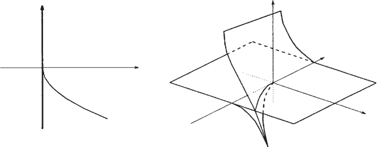
Figure 3: These figures correspond to Figures 2a) and 2b) in [7].

$\bullet$ The germs $g=v\pm u^{k}$, $k=2,3$.

Here $G(u,v,w,a)=v\pm u^{k}+a_{1}u+\ldots+a_{k-1}u^{k-1}$ and $F(x,y,a)=y^{2}\pm x^{k}+a_{1}x+\ldots a_{k-1}x^{k-1}$, which is the deformation of an $A_{k-1}$-singularity. $H(y,a)=y^{2}$ so $\mathscr{D}_{DPC}(G)$ is the plane $(a_{1},a_{2},0)$. Here $\mathscr{D}_{PD}(G)$ and $\mathscr{D}_{CE}(G)$ coincide.

For $k=2$, $\frac{\partial F}{\partial x}=\pm 2x+a_{1}=0$ and $\frac{\partial F}{\partial y}=2y=0$, so $\mathscr{D}_{PD}(G)$ is parametrised by

$$(\mp 2x,a_{2},\pm x^{2}).$$

See Figure 4 left, where the parameter $a_{2}$ is not shown.

For $k=3$, $\frac{\partial F}{\partial x}=\pm 3x^{2}+a_{1}+2a_{2}x=0$ and $\frac{\partial F}{\partial y}=2y=0$, so $\mathscr{D}_{PD}(G)$ is a cuspidal edge parametrised by

$$(\mp 3x^{2}-2a_{2}x,a_{2},\pm 2x^{3}-a_{2}x^{2}).$$

See Figure 4 right.

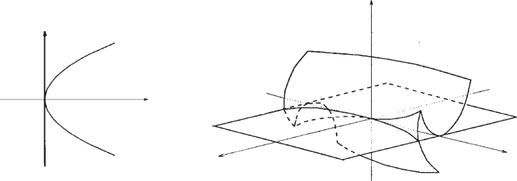
Figure 4: These figures correspond to Figures 3 and 4 in [7].

$\bullet$ The germ $g=w+u^{2}+buv+cv^{2}$.

Here $G(u,v,w,a)=w+u^{2}+buv+cv^{2}+a_{1}u+a_{2}v$ and $F(x,y,a)=xy^{3}+x^{2}+bxy^{2}+cy^{4}+a_{1}x+a_{2}y^{2}$. $\frac{\partial F}{\partial x}=y^{3}+2x+by^{2}+a_{1}=0$ and $\frac{\partial F}{\partial y}=3xy^{2}+2bxy+4cy^{3}+2a_{2}y=0$ which yields two solutions

$$\left\{\begin{array}[]{l}y=0\\ a_{1}=-2x\end{array}\right.\quad\text{and}\quad\left\{\begin{array}[]{l}a_{1}=-y^{3}-2x-by^{2}\\ a_{2}=-\dfrac{3}{2}xy-bx-2cy^{2},\end{array}\right.$$

so $\mathscr{D}_{PD}(G)$ has two components parametrised by

$$(-y^{3}-2x-by^{2},-bx-3/2xy-2cy^{2},-3/2xy^{3}-x^{2}-bxy^{2}-cy^{4}),$$

which is a cuspidal cross-cap, and

$$(-2x,a_{2},-x^{2}),$$

which is a hyperplane containing the cuspidal edge of the first component. The second component coincides with $\mathscr{D}_{CE}(G)$, which, in this case is contained in $\mathscr{D}_{PD}(G)$ (see Figure 5).

Figure 5: The discriminant $\mathscr{D}_{PD}(G)$. The dark part corresponds to $\mathscr{D}_{CE}(G)$.

On the other hand $H(y,a)=cy^{4}+a_{2}y^{2}$, so $\frac{\partial H}{\partial y}=4cy^{3}+2a_{2}y=0$, so $\mathscr{D}_{DPC}(G)$ consists of two components, the plane $(a_{1},a_{2},0)$ and another one parametrised by

$$(a_{1},-2cy^{2},-cy^{4}).$$

We can use these discriminants to study the dual of the cuspidal cross-cap. Consider again the height function $H_{{\bf v}}(x,y))=\phi(x,y)\cdot\bf v$. We have the sets

$$\mathscr{D}_{PD}(H)=\{({{\bf v}},H_{{\bf v}}(x,y))\in S^{2}\times\mathbb{R}:\frac{\partial H_{{\bf v}}}{\partial x}=\frac{\partial H_{{\bf v}}}{\partial y}=0\mbox{ at }(x,y,{{\bf v}})\},$$

$$\mathscr{D}_{DPC}(H)=\{({{\bf v}},H_{{\bf v}}(0,y))\in S^{2}\times\mathbb{R}:\frac{\partial H_{{\bf v}}}{\partial y}=0\mbox{ at }(0,y,{{\bf v}})\}$$

and

$$\mathscr{D}_{CE}(H)=\{({{\bf v}},H_{{\bf v}}(x,0))\in S^{2}\times\mathbb{R}:\frac{\partial H_{{\bf v}}}{\partial x}=0\mbox{ at }(x,0,{{\bf v}})\}.$$

If $\pi_{\bf v}$ is a member of the pencil containing the tangential direction of $M$ but is not the tangent cone to $M$, then the set $\mathscr{D}_{PD}(H)$ coincides with $\mathscr{D}_{CE}(H)$ and describes locally the dual of the curve $\Sigma$. When $\pi_{\bf v}$ is the tangent cone to $M$, then the set $\mathscr{D}_{PD}(H)$ consists of two components. One of them is $\mathscr{D}_{CE}(H)$ (the dual of $\Sigma$) and the other is the proper dual of $M$ which is the surface consisting of the tangent planes to $M$ away from points on $\Sigma$ together with their limits at points on $\Sigma$, i.e., the tangent cones at points on $\Sigma$. $\mathscr{D}_{DPC}(H)$ is the dual of the double point curve. If $\pi_{\bf v}$ is transversal to the limiting tangent vector of the double point curve, then $\mathscr{D}_{DPC}(H)$ consists of just one plane component. If $\pi_{\bf v}$ contains the limiting tangent vector of the double point curve, then $\mathscr{D}_{DPC}(H)$ consists of two components one of which is a plane.

If the contact of $M$ with $\pi_{{\bf v}}$ is described by that of the fibre $g=0$ with the model cuspidal edge $X$, with $g$ as in Theorem 3.6, then $\mathscr{D}_{PD}(H)$ (resp. $\mathscr{D}_{DPC}(H)$ and $\mathscr{D}_{CE}(H)$) is diffeomorphic to $\mathscr{D}_{PD}(G)$ (resp. $\mathscr{D}_{DPC}(G)$ and $\mathscr{D}_{CE}(G)$), where $G$ is an $\mathcal{R}^{+}(X)$-versal deformation of $g$ with 2-parameters.

Proposition 3.10.

The previous calculations give the generic models, up to diffeomorphisms, of $\mathscr{D}_{PD}(H)$, $\mathscr{D}_{DPC}(H)$ and $\mathscr{D}_{CE}(H)$, and these are as in Figures 3, 4 and 5.

4 The tangent developable surface of a space curve at a point of zero torsion

In [9], Cleave proved that the tangent developable surface of a space curve at a point of zero torsion has a cuspidal cross-cap singularity. In this section we study the geometry of such a cuspidal cross-cap.

Let $\gamma:I\to\mathbb{R}^{3}$ be a space curve, and $\gamma=(\gamma_{1},\gamma_{2},\gamma_{3})$. Without loss of generality we assume that $\gamma$ is transverse to the plane $X=0$, namely, $\gamma_{1}^{\prime}(0)\neq 0$. Then there exists a parameter $u$ such that $\gamma(u)=(u,\gamma_{2}(u),\gamma_{3}(u))$. Let $f$ be the tangent developable surface of $\gamma$:

$$f(u,v)=(u+v,\gamma_{2}(u)+v\gamma_{2}^{\prime}(u),\gamma_{3}(u)+v\gamma_{3}^{\prime}(u)).$$

Thus, if $\det(\tilde{\gamma}^{\prime}(0),\tilde{\gamma}^{\prime\prime}(0))\neq 0$, then $0$ is a singularity of the first kind, where $\tilde{\gamma}=(\gamma_{2},\gamma_{3})$. In what follows, we assume $\det(\tilde{\gamma}^{\prime}(0),\tilde{\gamma}^{\prime\prime}(0))\neq 0$. We have

$$\lambda=v,\quad\eta=\partial_{u}-\partial_{v}.$$

Let $\kappa_{s}^{f},\kappa_{\nu}^{f},\kappa_{t}^{f},\kappa_{c}^{f}$ be the invariants $\kappa_{s},\kappa_{\nu},\kappa_{t}$ and $\kappa_{c}$, of $f$.

Then we have

$$\kappa_{s}^{f} =-\dfrac{\sqrt{(1+(\gamma_{2}^{\prime})^{2})(\gamma_{3}^{\prime\prime})^{2}-2\gamma_{3}^{\prime}\gamma_{2}^{\prime}\gamma_{3}^{\prime\prime}\gamma_{2}^{\prime\prime}+(1+(\gamma_{3}^{\prime})^{2})(\gamma_{2}^{\prime\prime})^{2}}}{(1+(\gamma_{3}^{\prime})^{2}+(\gamma_{2}^{\prime})^{2})^{3/2}}=\kappa$$

$$\kappa_{\nu}^{f} =0$$

$$\kappa_{t}^{f} =\dfrac{-\gamma_{2}^{\prime\prime}\gamma_{3}^{\prime\prime\prime}+\gamma_{3}^{\prime\prime}\gamma_{2}^{\prime\prime\prime}}{(\gamma_{3}^{\prime\prime})^{2}+(\gamma_{2}^{\prime\prime})^{2}+(\gamma_{2}^{\prime}\gamma_{3}^{\prime\prime}-\gamma_{3}^{\prime}\gamma_{2}^{\prime\prime})^{2}}=\tau$$

$$\kappa_{c}^{f} =\dfrac{2(1+(\gamma_{3}^{\prime})^{2}+(\gamma_{2}^{\prime})^{2})^{3/2}(-\gamma_{2}^{\prime\prime}\gamma_{3}^{\prime\prime\prime}+\gamma_{3}^{\prime\prime}\gamma_{2}^{\prime\prime\prime})}{((\gamma_{3}^{\prime\prime})^{2}+(\gamma_{2}^{\prime\prime})^{2}+(\gamma_{2}^{\prime}\gamma_{3}^{\prime\prime}-\gamma_{3}^{\prime}\gamma_{2}^{\prime\prime})^{2})^{5/2}}.$$

where $\kappa$ and $\tau$ are the curvature and the torsion of the space curve $f(u,0)=\gamma(u)$. If $\tau(0)=0$, then $f(u,v)$ has a cuspidal cross-cap singularity at the origin and $\kappa_{\nu}(0)=\kappa_{t}(0)=\kappa_{c}(0)=0$. Therefore, from the point of view of its invariants, this cuspidal cross-cap is not generic, since there are cuspidal cross-caps with $\kappa_{\nu}\neq 0$ and $\kappa_{t}\neq 0$.

However, we can consider the contact of this cuspidal cross-cap with planes. The tangent cone of $f$ contains $\gamma^{\prime}(0)=(1,0,0)$. Consider the contact of $f$ with its tangent cone, that is, take a direction ${\bf v}=(0,v_{2},v_{3})$ and consider the height function

$$H_{{\bf v}}(x,y)=(\gamma_{2}(u)+v\gamma_{2}^{\prime}(u))v_{2}+(\gamma_{3}(u)+v\gamma_{3}^{\prime}(u))v_{3}.$$

Notice that $H$ can never have an $A_{3}$-singularity, which is the only generic singularity of the height function which cannot be recovered by folding a cuspidal edge (see Remark 3.9 i)). This suggests that any cuspidal cross-cap obtained from the tangent developable of a space curve at a point of zero torsion, which is generic in the sense of its contact with planes, can be obtained by folding a cuspidal edge.

ROS: Departament de Matemàtiques, Universitat de València, c/ Dr Moliner no 50, 46100, Burjassot, València, Spain.
Email: raul.oset@uv.es

KS: Department of Mathematics, Kobe University, Rokko 1-1, Nada, Kobe 657-8501, Japan
Email: saji@math.kobe-u.ac.jp

References

- [1] V. I. Arnol ’ d, Reconstructions of singularities of potential flows in a collision-free medium and caustic metamorphoses in three-dimensional space. (Russian) Trudy Sem. Petrovsk. No. 8 (1982), 21–57.
- [2] V. I. Arnol ’ d, Singularities of caustics and wave fronts. Volume 62 of Mathematics and its Applications (Soviet Series) . Kluwer Academic Publishers Group, Dordrecht, 1990.
- [3] M. Barajas Sichaca, Folding maps on a crosscap. Preprint, 2017.
- [4] M. Barajas Sichaca and Y. Kabata, Projections of the cross-cap. Preprint, 2017.
- [5] J. W. Bruce, N. P. Kirk and A. A. du Plessis, Complete transversals and the classification of singularities. Nonlinearity 10 (1997), 253–275.
- [6] J. W. Bruce and R. M. Roberts, Critical points of functions on analytic varieties. Topology 27 (1988), 57–90.
- [7] J. W. Bruce and J. M. West, Functions on a crosscap. Math. Proc. Cambridge Philos. Soc. 123 (1998), 19–39.
- [8] J. W. Bruce and T. C. Wilkinson, Folding maps and focal sets. Lecture Notes in Math., 1462, 63–72, Springer, Berlin, 1991.
- [9] J. P. Cleave, The form of the tangent-developable at points of zero torsion on space curves. Math. Proc. Cambridge Philos. Soc. 88 (1980), no. 3, 403–407.
- [10] J. N. Damon, Topological triviality and versality for subgroups of and . Mem. Amer. Math. Soc. 75 (1988), no. 389.
- [11] A. A. Davydov, Normal form of slow motions of an equation of relaxation type and fibering of binomial surfaces. (Russian) Mat. Sb. (N.S.) 132(174) (1987), no. 1, 131–139, 143; translation in Math. USSR-Sb. 60 (1988), no. 1, 133–141.
- [12] F. S. Dias and F. Tari, On the geometry of the cross-cap in Minkowski 3-space and binary differential equations. Tohoku Math. J. (2) 68 (2016), no. 2, 293–328.
- [13] T. Fukui and M. Hasegawa, Fronts of Whitney umbrella – a differential geometric approach via blowing up. J. Singul. 4 (2012), 35–67.
- [14] M. Hasegawa, A. Honda, K. Naokawa, M. Umehara and K. Yamada, Intrinsic invariants of cross caps. Selecta Math. (N.S.) 20 (2014), no. 3, 769–785.
- [15] M. Hasegawa, A. Honda, K. Naokawa, K. Saji, M. Umehara and K. Yamada, Intrinsic properties of surfaces with singularities. Internat. J. Math. 26 (2015), no. 4, 1540008, 34 pp.
- [16] A. Honda, K. Naokawa, M. Umehara and K. Yamada, Isometric realization of cross caps as formal power series and its applications, arXiv:1601.06265.
- [17] A. Honda and K. Saji, Geometric invariants of -cuspidal edges, arXiv:1710.06014.
- [18] S. Izumiya, M. Takahashi and F. Tari, Folding maps on spacelike and timelike surfaces and duality. Osaka J. Math. 47 (2010), no. 3, 839–862.
- [19] S. Izumiya, M. C. Romero Fuster, M. A. S. Ruas and F. Tari, Differential geometry from singularity theory viewpoint. World Scientific Publishing Co. Pte. Ltd., Hackensack, NJ, 2016.
- [20] N. P. Kirk, Computational aspects of classifying singularities. LMS J. Comput. Math. 3 (2000), 207–228.
- [21] M. Kokubu, W. Rossman, K. Saji, M. Umehara and K. Yamada, Singularities of flat fronts in hyperbolic space. Pacific J. Math. 221 (2005), no. 2, 303–351.
- [22] L. Martins and J. J. Nuño Ballesteros, Contact properties of surfaces in with corank 1 singularities. Tohoku Math. J. 67 (2015), 105–124.
- [23] L. Martins and K. Saji, Geometric invariants of cuspidal edges. Canad. J. Math. 68 (2016), 445–462.
- [24] L. Martins and K. Saji, Geometry of cuspidal edges with boundary. Preprint. arXiv:1610.09808
- [25] L. F. Martins, K. Saji, M. Umehara and K. Yamada, Behavior of Gaussian curvature and mean curvature near non-degenerate singular points on wave fronts, Geometry and topology of manifolds, 247–281, Springer Proc. Math. Stat., 154, Springer, Tokyo, 2016.
- [26] K. Naokawa, M. Umehara and K. Yamada, Isometric deformations of cuspidal edges. Tohoku Math. J. 68 (2016), 73–90.
- [27] J. J. Nuño-Ballesteros and F. Tari, Surfaces in and their projections to 3-spaces. Proc. Roy. Soc. Edinburgh Sect. A 137 (2007), no. 6, 1313–1328.
- [28] J. M. Oliver, On pairs of foliations of a parabolic cross-cap. Qual. Theory Dyn. Syst. 10 (2011), no. 1, 139–166.
- [29] R. Oset Sinha and F. Tari, Projections of surfaces in to and the geometry of their singular images. Rev. Mat. Iberoam. 31 (2015), no. 1, 33–50.
- [30] R. Oset Sinha and F. Tari, Flat geometry of cuspidal edges. To appear in Osaka J. Math.
- [31] G. Peñafort-Sanchis, Reflection maps. Preprint. arXiv:1609.03222
- [32] K. Saji, Criteria for cuspidal singularities and their applications. J. Gokova Geom. Topol. GGT 4, 67-81 (2010).
- [33] K. Saji, M. Umehara and K. Yamada, singularities of wave fronts. Math. Proc. Cambridge Philos. Soc. 146 (2009), no. 3, 731–746.
- [34] K. Saji, M. Umehara, and K. Yamada, The geometry of fronts. Ann. of Math. (2) 169 (2009), 491–529.
- [35] K. Saji, M. Umehara, and K. Yamada, Coherent tangent bundles and Gauss-Bonnet formulas for wave fronts. J. Geom. Anal. 22 (2012), no. 2, 383–409.
- [36] I. R. Shafarevich, Basic algebraic geometry. 1. Varieties in projective space. Third edition. Springer, Heidelberg, 2013.
- [37] K. Teramoto, Parallel and dual surfaces of cuspidal edges. Differential Geom. Appl. 44 (2016), 52–62.
- [38] J. M. West, The differential geometry of the crosscap. Ph.D. thesis, The University of Liverpool, 1995.
- [39] V. M. Zakalyukin and A. O. Remizov, Legendre singularities in systems of implicit ordinary differential equations and fast-slow dynamical systems. (Russian) Tr. Mat. Inst. Steklova 261 (2008), Differ. Uravn. i Din. Sist., 140–153 ISBN: 978-5-7846-0106-3 ; translation in Proc. Steklov Inst. Math. 261 (2008), no. 1, 136–148.