Unifying static and dynamic properties in 3D quantum antiferromagnets

Abstract

Quantum Monte Carlo simulations offer an unbiased means to study the static and dynamic properties of quantum critical systems, while quantum field theory provides direct analytical results. We study three dimensional, critical quantum antiferromagnets by performing a combined analysis using both quantum field theory calculations and quantum Monte Carlo data. Explicitly, we analyze the order parameter (staggered magnetization), Néel temperature, quasiparticle gaps, and the susceptibilities in the scalar and vector channels. We connect the two approaches by deriving descriptions of the quantum Monte Carlo observables in terms of the quasiparticle excitations of the field theory. The remarkable agreement not only unifies the description of the static and dynamic properties of the system, but also constitutes a thorough test of perturbative O(3) quantum field theory and opens new avenues for the analytical guidance of detailed numerical studies.

I Introduction

Quantum field theories (QFTs) are of fundamental importance to both high-energy and statistical physics. In particular, the generic O($N$)-symmetric, $d$-dimensional field theory finds a remarkably broad application. For $N=0$ this theory describes the self-avoiding random-walk problem, while for $N=1$, $2$, and $3$ it describes magnetic models with, respectively, Ising, XY, and Heisenberg interactions. In nuclear physics, the $N=4$ version in $d=4$ dimensions is of particular importance because it provides an effective theory for $\pi$-mesons. Taking $N\rightarrow\infty$, one obtains the spherical model Zinn-Justin (2002).

In the vicinity of a classical or a quantum phase transition (QPT), any characteristic length scale of a physical system diverges Sachdev (2011). If the system is described by a QFT, its properties then depend solely on the dimensionality, $d$, and the internal symmetries, which for O($N$) theories means the number of components, $N$. These provide a unique determination of the universality class and hence of the critical exponents of the field theory at the QPT. The robust predictions of QFT in this regard have inspired a multitude of experimental and numerical studies, and in fact constitutes an entire subfield of physics.

Quite generally, quantum systems in high dimensions have sufficiently many degrees of freedom that their behavior is “free,” governed by the same set of exponents that can be derived at the mean-field level. Systems in low dimensions are constrained and their exponents are “anomalous,” depending in detail on $d$, $N$, and the form of the interaction terms. A situation of special importance occurs for systems at the upper critical dimension, $d_{c}=4$, which in the quantum case is often expressed as $3+1$ [for three spatial and one temporal dimension(s)]. Here the critical exponents are predicted to take mean-field values, which for O($N$) field theories are independent of $N$, augmented by multiplicative logarithmic corrections to the observables. Because an explicit $N$-dependence does appear in the multiplicative logarithmic corrections, these represent a fundamental test of universality Zinn-Justin (2002); Kenna and Lang (1993, 1994) and their existence has profound consequences in both high-energy and statistical physics.

Although there exists a wealth of analytical results detailing the theory of logarithmic corrections Zinn-Justin (2002); Wegner and Riedel (1973); Domb et al. (1976); Hara and Tasaki (1987); Fernández et al. (1992); Li and Chen (1997); Kleinert and Schulte-Frohlinde (2001), discerning them in experimental measurements is a hugely demanding task requiring datasets spanning many orders of magnitude in parameter space near a QPT. Similarly, their numerical determination in lattice simulations is a delicate and highly computationally intensive proposition. Numerical tests of logarithmic corrections have mostly been restricted to the $N=1$ theory Kenna and Lang (1993, 1994, 1994); de Forcrand et al. (2010), and only recently has a movement beyond $N=1$ been driven by a confluence of refined numerical methods, increasing computer power, and rising interest from experiments in condensed matter Sachdev . Experimental studies of QPTs were motivated initially by problems in superconductivity, where the order parameter has U(1) or equivalently O(2) symmetry, and have since broadened to include quantum magnetism, where the order parameter in the Heisenberg case has O(3) symmetry Chakravarty et al. (1988), and condensates of ultracold atoms, in which different symmetries can be realized. In all cases the system dimensionality is $d=1$, 2, or 3.

Here we specialize to the case of quantum antiferromagnets (QAFs). Critical magnetic systems in the $d=2+1$, $N=3$ universality class have been the object of extensive numerical Sandvik and Scalapino (1994); Troyer et al. (1996); Matsumoto et al. (2001); Wang et al. (2006); Wenzel and Janke (2009) and analytical Podolsky et al. (2011); Podolsky and Sachdev (2012); Gazit et al. (2013a, b); Rançon and Dupuis (2014) investigation for over two decades, and have undergone a recent revival due to their close parallels in ultracold atomic experiments. However, our present focus is the $d=3+1$, $N=3$ QPT, which on the theoretical side encompasses all the physics of the upper critical dimension and on the experimental side is realized in the compound TlCuCl₃. TlCuCl₃ is a $S=1/2$ QAF with a dimerized geometry and three-dimensional (3D) interdimer coupling, which can be driven by an applied hydrostatic pressure through a QPT between a magnetically ordered AF phase and a “quantum disordered” dimerized phase. Elastic and inelastic neutron scattering experiments on TlCuCl₃ Rüegg et al. (2004, 2008); Merchant et al. (2014) have characterized clearly the hallmarks of the magnetic QPT in both the static and dynamic properties.

From the viewpoint of QFT, the 3D dimerized QAF provides an excellent test case for the study of critical properties around the QPT at $d_{c}$. The weakness of QFTs is that, as effective low-energy, long-wavelength theories, their connection to real systems is only through phenomenological parameters, and thus it is essential to benchmark them against numerical and experimental realizations. Indeed the effective O(3), $d=3+1$ QFT has already been used to provide an accurate analytical description of the critical properties observed in TlCuCl₃ Sachdev ; Kulik and Sushkov (2011); Scammell and Sushkov (2015); Katan and Podolsky (2015); Scammell and Sushkov (2017a); Fidrysiak and Spałek (2017). Numerically, the method of choice for computing the properties of the unfrustrated QAF is Quantum Monte Carlo (QMC), with which recent large-scale simulations of the 3D dimerized QAF across the quantum critical regime have been performed for $S=1/2$ spins with Heisenberg interactions on the double-cubic geometry depicted in Fig. 1(a). First a systematic study of the static properties by some of us Qin et al. (2015) demonstrated to high precision the validity of the theoretical predictions concerning multiplicative logarithmic corrections for this universality class. Next, two parallel studies Qin et al. (2017); Lohöfer and Wessel (2017) used QMC and analytic continuation methods to access the dynamical properties of the system. The aim of the present work is, within a one-loop perturbative renormalization-group (RG) treatment of the O(3), $d=3+1$ QFT, to analyze and unify the static and dynamic observables obtained in these QMC simulations.

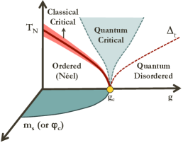
In the vicinity of the magnetic quantum critical point (QCP), the observables accounting for the relevant (critical) degrees of freedom are associated with the broken or unbroken O(3) symmetry. In the symmetric (quantum disordered) phase there are three degenerate, gapped spin excitations, which because of their triplet character are known as triplons; their energy gap, denoted by $\Delta$ in Fig. 1(b), closes as the QCP is approached. In the symmetry-broken phase, a preferred direction is established and is associated with an order parameter, which for a QAF is the staggered magnetization, $m_{s}$. In three spatial dimensions, magnetic order is present up to a finite Néel temperature, $T_{N}$, at which it is destroyed by thermal fluctuations. An illustration of the phase diagram and the behavior of these observables is presented in Fig. 1(b).

Figure 1: (a) Dimerized lattice of $S=1/2$ spins in the 3D double-cubic geometry. Sites of the red and blue cubic lattices are connected pairwise by dimer bonds. $J^{\prime}$ and $J$ are antiferromagnetic Heisenberg interactions respectively on and between the dimer units. Their ratio, $g=J^{\prime}/J$, controls the QPT from a Néel ordered phase (left) to a quantum disordered dimer-singlet phase (right). The QCP occurs at the critical ratio $g_{c}$. (b) Schematic quantum critical phase diagram for the Heisenberg model on the double-cubic lattice. The staggered magnetization, $m_{s}$ (or $\varphi_{c}$), Néel temperature, $T_{N}$, and triplon gap, $\Delta_{t}$, all vanish at the QCP. Not shown is the Higgs gap, $\Delta_{H}$, which is proportional to $\varphi_{c}$ and hence also vanishes at the QCP.

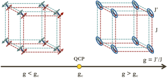
Directional oscillations of the order parameter are acoustic (gapless) and are are known as Goldstone modes. Their linear dispersion about the gapless point ensures that the dynamical critical exponent is $z=1$, and hence that the time axis counts as one additional system dimersion. By contrast, the amplitude oscillation of the order parameter is a gapped mode, often referred to as the “Higgs mode” by analogy with the amplitude modes in a superconductor and in electroweak field theory, although in the QAF it lacks the gauge character of these two systems. In the O(3) case there are two Goldstone modes and one Higgs, such that the three modes of the phases on either side of the QPT evolve continuously evolve into each other at the QCP. Because of its finite gap, or mass, it is possible in the O(3) QFT for the Higgs mode to decay spontaneously into Goldstone modes, and therefore it has not only an energy but also an intrinsic line width.

QFT and QMC both provide direct access to the static quantities of the system, namely the staggered magnetization and Néel temperature, and to the dynamic ones, which are the characteristic energy gaps of the triplon and Higgs modes, as well as the Higgs decay width. In QMC, the static and dynamic quantities are treated on a quite unequal footing, requiring very different techniques to extract. By contrast, they appear in a completely symmetric way in a QFT and thus are treated on an equal footing, being equivalently and uniquely determined by a set of (five) phenomenological QFT parameters. However, where a QFT is an effective low-energy theory, the applicability of QMC is by no means limited to the low-energy sector, nor by any of the other approximations inherent to QFT, and in this sense QMC is a completely unbiased method.

The static Qin et al. (2015) and dynamic Qin et al. (2017); Lohöfer and Wessel (2017) observables computed by QMC on both sides of the QCP for the double-cubic QAF have each been shown to fit the universal scaling forms expected from the O(3) QFT with $d=3+1$ Zinn-Justin (2002), including their logarithmic corrections. Nevertheless, important questions remain for both QMC and QFT. Specifically, space-time symmetry is largely lost in QMC, and with it any underlying connection between static and dynamic variables. While QFT is in principle perfectly suited for retrieving this connection, it has yet to be determined whether or not all of the observables of the system can be described quantitatively by an effective low-energy QFT with a single set of phenomenological parameters. An alternative statement of our primary goal is to derive this single set of parameters.

Further, the Higgs line width is an important additional observable but its determination lies at the limits of current numerical capabilities. The vector and scalar response functions used to compute the Higgs decay rate in the recent QMC studies Qin et al. (2017); Lohöfer and Wessel (2017) are described naturally by QFT in terms of the Green functions, or generalized response functions, of the magnetic excitations (the Goldstone and Higgs modes). Thus one may perform a detailed analysis of the vector and scalar response functions to obtain analytical guidance for interpreting the existing QMC line-width data and for structuring future numerical studies.

This paper is organized as follows. In Sec. II we present the lattice Hamiltonian we study, summarize the QMC methods we have applied and the nature of their output, formulate the QFT description at the mean-field level, and detail the process for computing one-loop RG corrections. In Sec. III we apply the analytical QFT formulas to fit the static and dynamic QMC data of Refs. Qin et al. (2015, 2017) and extract the phenomenological QFT parameters. Section IV provides a detailed analysis of the vector and scalar response functions, with which we analyze the Higgs line width for comparison with QMC Qin et al. (2017). For completeness, in Sec. V we relate the optimal QFT parameters to the analogous quantities derived from a microscopic description, for which we use a bond-operator framework. In Sec. VI we discuss the context of our results and their value for future research directions.

II Model and Methods

The double-cubic geometry, shown in Fig. 1(a), is perhaps the most representative and spatially symmetric 3D dimerized lattice. This system consists of two interpenetrating simple cubic lattices with the same antiferromagnetic interaction strength, $J$, connected pairwise by another antiferromagnetic interaction, $J^{\prime}$; there is no frustration in this situation. The ground state for low coupling ratios, $g=J^{\prime}/J$, is a Néel-ordered phase of finite staggered magnetization and for high $g$ it is dimer-singlet phase with no order, as illustrated in Fig. 1(b). The critical coupling ratio for the QPT is denoted by $g_{c}$. The Hamiltonian is

$$H=J\sum_{<i,j>}\{\bm{S}_{l}^{i}\cdot\bm{S}_{l}^{j}+\bm{S}_{r}^{i}\cdot\bm{S}_{r}^{j}\}+J^{\prime}\sum_{i}\bm{S}_{l}^{i}\cdot\bm{S}_{r}^{i},$$ (1)

where the subscripts $l$ and $r$ denote the two spins on a single dimer bond.

Supplemented by an appropriate treatment of the temperature, Eq. (1) contains all of the information about the static and dynamic observables of the system, whose qualitative behavior is depicted in Fig. 1(b). We summarize the two parallel techniques we employ here to extract those observables, namely direct numerical QMC simulation augmented by stochastic analytic continuation (SAC), and the analysis of the effective low-energy QFT derived from Eq. (1). Both QMC and QFT techniques allow for the efficient inclusion of finite temperatures in the quantum system, albeit in very different ways we outline below.

II.1 Quantum Monte Carlo

We have performed QMC simulations using the stochastic series expansion (SSE) technique Sandvik and Kurkijärvi (1991); Sandvik (1999); Evertz (2003). In this method, spin configurations are constructed in the $S^{z}$ basis, evolved over an imaginary time $\tau$, and sampled systematically. The (squared) order parameter is evaluated straightforwardly from the spatial and temporal average of $S_{i}^{lz}(\tau)-S_{i}^{rz}(\tau)$ and dynamical correlation functions are obtained from operator strings connecting states $S_{i}^{lz}(\tau_{1})-S_{i}^{rz}(\tau_{1})$ and $S_{j}^{lz}(\tau_{2})-S_{j}^{rz}(\tau_{2})$. To avoid the repetition of published material, we refer the reader to Ref. Qin et al. (2015). To evaluate the static quantities, we have performed simulations on cubic systems of $2L^{3}$ sites for values of $L$ up to and including 48, and at temperatures down to $1/2L$. By detailed finite-size scaling we extrapolate to the thermodynamic limit to obtain unbiased results with well-controlled statistical errors. We comment that the errors on $m_{s}$ in the ordered phase, which extrapolates to a finite zero-temperature quantity for all $g<g_{c}$, are significantly smaller than the errors on $T_{N}$, which are determined from the vanishing of $m_{s}$ at finite temperatures.

In order to obtain the dynamical response of the system, we first measure the imaginary-time structure factor and then employ SAC Sandvik (1998); Beach ; Syljuåsen (2008); Fuchs et al. (2010); Sandvik (2016) to obtain the real-frequency spectral function. This process can be performed using both the spin operator, $S_{i}^{lz}(\tau)-S_{i}^{rz}(\tau)$, and the dimer operator, $B_{i}(\tau)=\bm{S}_{i}^{l}(\tau)\cdot\bm{S}_{i}^{r}(\tau)-\langle\bm{S}_{i}^{l}(\tau)\cdot\bm{S}_{i}^{r}(\tau)\rangle$. The spin spectral function is referred to as the vector response function or the $S=1$ channel and the dimer spectral function as the scalar response function or $S=0$ channel. Again we refer the reader to previously published material Qin et al. (2017). Because the extraction of dynamical quantities is considerably more computationally intensive, our maximum $L$ is limited to 24 and the errors in extrapolated quantities are correspondingly larger, but still well characterized. In these simulations the excitation gaps, $\Delta_{t}$ for the triplons at $g>g_{c}$ and $\Delta_{H}$ for the Higgs mode at $g<g_{c}$, are obtained with significantly greater accuracy than the Higgs line width, $\Gamma_{H}$, obtained from either channel. We note that the present study does not involve any new simulations, but that we have reanalyzed some of our existing data Qin et al. (2015, 2017) in the light of the comparison with QFT.

At zero temperature and in the quantum critical regime, the observables $m_{s}$, $\Delta_{t}$, and $\Delta_{H}$ have the generic form of a power-law dependence on the separation from the QCP, $\delta g=(g-g_{c})/g_{c}$, multiplied by a logarithmic correction Zinn-Justin (2002); Scammell and Sushkov (2015); Qin et al. (2015, 2017); Lohöfer and Wessel (2017). We express them in the form

$$m_{s}(g) =a_{1}|g-g_{c}|^{\nu_{1}}\ln\left[\frac{|g-g_{c}|}{b_{1}}\right]^{\beta_{1}},$$ (2)

$$\Delta_{t}(g) =a_{2}|g-g_{c}|^{\nu_{2}}\ln\left[\frac{|g-g_{c}|}{b_{2}}\right]^{\beta_{2}},$$ (3)

$$\Delta_{H}(g) =a_{3}|g-g_{c}|^{\nu_{3}}\ln\left[\frac{|g-g_{c}|}{b_{3}}\right]^{\beta_{3}}.$$ (4)

At finite temperatures, the Néel temperature can be expressed in the same manner Qin et al. (2015); Scammell and Sushkov (2015), as

$$T_{N}(g) =a_{4}|g-g_{c}|^{\nu_{4}}\ln\left[\frac{|g-g_{c}|}{b_{4}}\right]^{\beta_{4}}.$$ (5)

The quantum critical behavior is then gathered in the exponents $\nu_{i}$ for the power-law dependence and $\beta_{i}$ for the multiplicative logarithmic correction. The exponents $\{\nu_{i},\beta_{i}\}$ have received a great deal of attention and have been discussed by scaling hypotheses and general QFT arguments for many different universality classes. At the upper critical dimension, $\nu_{i}=1/2$, i.e. all observables follow a predominantly mean-field form, independent of $N$. For an O($N$) system at $d_{c}$, the static observables have $\beta_{1}=\beta_{4}=3/(N+8)$ at one-loop order and the dynamic observables have $\beta_{2}=\beta_{3}=-(N+2)/2(N+8)$ Zinn-Justin (2002). Although these critical exponents have been verified to high precision by the recent QMC analyses Qin et al. (2015, 2017); Lohöfer and Wessel (2017), the relationships among the coefficients $\{a_{i},b_{i}\}$ remains unknown and can be determined by appealing to QFT.

II.2 Quantum field theory: Mean-field treatment

To capture the ordered and disordered phases, the QPT between them, and the low-energy magnetic degrees of freedom, we adopt the effective description of the Hamiltonian (1) provided by the Lagrangian field theory Sachdev (2011)

$${\cal L} ={\textstyle\frac{1}{2}}\partial_{\mu}{\vec{\varphi}}\,\partial^{\mu}{\vec{\varphi}}-{\textstyle\frac{1}{2}}m^{2}{\vec{\varphi}}^{\ 2}-{\textstyle\frac{1}{4}}\alpha[\vec{\varphi}^{\ 2}]^{2}.$$ (6)

Here $\vec{\varphi}$ is a vector field describing the staggered magnetization, $m$ is a mass term for free field fluctuations, $\alpha$ is a stiffness term governing the interactions of $\vec{\varphi}$ fluctuations, and the index $\mu$ enumerates one time and three space coordinates, with $\partial_{\mu}=(\partial_{t},c\nabla)$, where the constant of proportionality, $c$, is the velocity of the Goldstone modes in the ordered phase. For later quantitative purposes (Secs. II.3 and IIIA) we note that $m$ is defined to have units of energy (and $\alpha$ of an energy cubed).

Qualitatively, the QPT is controlled in Eq. (6) through the mass term, which we express at linear order as $m^{2}(\delta g)=\gamma^{2}(g-g_{c})/g_{c}$, where $\gamma^{2}>0$ is another constant of proportionality. For $g>g_{c}$, $m^{2}>0$ and the classical expectation value of the field is $\varphi_{c}^{2}=0$, which describes the magnetically disordered phase. The system has a global rotational symmetry and its excitations (the triplons) are gapped and triply degenerate. For $g<g_{c}$, $m^{2}<0$ and the (staggered) field takes a non-zero classical expectation value, $\varphi^{2}_{c}=|m^{2}|/\alpha$, which describes the ordered antiferromagnetic phase. Changing $m^{2}$ from positive to negative causes a spontaneous breaking of the O(3) spin symmetry and the excitations of the symmetry-broken phase are two gapless, transverse excitations (spin waves, the Goldstone modes) and one gapped, longitudinal excitation (the amplitude or Higgs mode). It is straightforward using the bare (unrenormalized) parameters to note that the triplon gap (at $g>g_{c}$) is $\Delta_{t}(\delta g)=m(\delta g)$ and the Higgs gap (at $g<g_{c}$) is $\Delta_{H}(\delta g)=\sqrt{2}|m(\delta g)|$, and hence to recover the relation $\Delta_{H}/\Delta_{t}=\sqrt{2}$.

Figure 2: Diagrammatic expansions for (a) the four-point vertex, $\Gamma^{(4)}$, and (b) the response function, $\chi_{\varphi\varphi}$, shown for the quantum disordered phase ($g>g_{c}$). Solid lines denote the free propagation, governed by the first two terms of Eq. (6), of the field $\varphi$, which here corresponds to triplon propagation. The vertex marked by the solid circle represents the bare interaction, the third term of Eq. (6), whose coefficient, $\alpha$, is the perturbative parameter. The one-loop corrections to $\Gamma^{(4)}$ and $\chi_{\varphi\varphi}$ are equivalent to retaining next-to-leading-order terms in $\alpha$. For the expansion of $\Gamma^{(4)}$ this implies $\alpha^{2}$ terms, which are contained in the three distinct loop diagrams (the Mandelstam s, t, and u channels) in panel (a). For the expansion of $\chi_{\varphi\varphi}$ this is the order-$\alpha$ loop diagram in panel (b), to which we refer as the self-energy, $\Sigma$. The perturbative RG treatment of $\Gamma^{(4)}$ and $\chi_{\varphi\varphi}$ (Sec. II.3) determines the running coupling constant (8) and the running mass (12) of the QFT description.

This mean-field analysis accounts for neither quantum nor thermal fluctuations. These we include in the present analysis at one-loop order, meaning that we consider contributions from the vertex and self-energy diagrams shown in Fig. 2. To provide a self-contained treatment, in Sec. II.3 we demonstrate the procedure for the RG resummation, by which we obtain the one-loop quantum and thermal corrections that are central to the analysis of Secs. III and IV.

II.3 Quantum field theory: One-loop corrections

The purpose of the present study is to obtain explicit expressions for the order parameter, excitation gaps, and Néel temperature, and hence all of their critical exponents, within the one-loop RG treatment of the QFT. To derive an analytic expression for the Néel temperature on the same footing as the zero-temperature quantities, it is necessary also to extend the analysis to finite temperatures. We take $J=1$ as the unit of energy and set the fundamental constants $\hbar=1$ and $k_{\rm B}=1$. In the QFT, $\omega_{k}=\sqrt{c^{2}k^{2}+m^{2}}$ is the energy of a magnetic excitation at momentum (wave vector) ${\bm{k}}$, which is measured from the antiferromagnetic ordering wave vector, ${\bm{Q}}=(\pi,\pi,\pi)$. This matches the low-energy form of gapped or gapless spin excitations in the starting Hamiltonian (1), while details of the higher-lying band excitations are not relevant to QFT.

II.3.1 Renormalization and Running Coupling

We generalize the 3+1D QFT to an O($N$) theory and demonstrate the renormalization of the coupling constant, $\alpha$, of the Lagrangian (6) by considering the quantum disordered phase ($g>g_{c}$). The requirements of energetic scale-invariance give rise to the RG treatment of the QFT. We illustrate the RG process by evaluating the one-loop correction to the four-point vertex shown in Fig. 2,

$$\Gamma^{(4)} =6\alpha+6(N+8)\,\alpha^{2}\int^{\Lambda_{c}}_{\Lambda}\frac{d^{4}k}{(2\pi)^{4}c^{3}}\frac{i}{(k^{2}-m^{2})^{2}}$$

$$=6\alpha-\frac{6(N+8)\,\alpha^{2}}{8\pi^{2}c^{3}}\ln\left[\frac{\Lambda_{c}}{\Lambda}\right]$$ (7)

if $\Lambda\geq m$. Here $k^{2}=\omega^{2}-c^{2}{\bm{k}}^{2}$ is the square of the four-momentum, the factor of $1/c^{3}$ arises from rescaling the integration measure, and $m$ serves as the lower bound of the infrared cutoff, $\Lambda$. The first term in Eq. (7) corresponds to the first diagram in the perturbative series for $\Gamma^{(4)}$ represented in Fig. 2(a) and the second to the three O($\alpha^{2}$) diagrams. A detailed discussion of the four-point vertex may be found in Ref. Kleinert and Schulte-Frohlinde (2001); the common factor of 6 is absorbed in constants of proportionality and the universal factor of $(N+8)$ accounts for the number of inequivalent diagrams contributing at this order.

The primary purpose of renormalization is to control the ultraviolet divergence, which is expressed in Eq. (7) by $\Lambda_{c}$; in a lattice problem such as the double-cubic model, the ultraviolet momentum cut-off is the inverse lattice spacing. The beta function of the RG flow is obtained from the Callan-Symanzik equation,

$$\left[\frac{d}{d\ln(\Lambda_{c}/\Lambda)}+\beta(\alpha)\frac{d}{d\alpha}\right]\Gamma^{(4)} =0$$

whence

$$\beta(\alpha) =\frac{(N+8)\alpha^{2}}{8\pi^{2}c^{3}}$$

$$\frac{d\alpha}{d\ln(\Lambda_{0}/\Lambda)} =-\frac{(N+8)\alpha^{2}}{8\pi^{2}c^{3}}$$

$$\alpha(\Lambda)\equiv\alpha_{\Lambda} =\frac{\alpha_{0}}{1+\frac{(N+8)}{8\pi^{2}c^{3}}\alpha_{0}\ln(\Lambda_{0}/\Lambda)}.$$ (8)

This demonstrates explicitly how the RG procedure removes the dependence on $\Lambda_{c}$ by introducing a normalization point, $\Lambda_{0}$, which is a parameter that can be fixed by optimizing the fit to the starting model. The RG equations nevertheless retain a dependence on the infrared energy scale, $\Lambda$, which is the actual energy scale of the QFT and is set by the physical energy scale of the system. Because this is either the mass (gap) of the field $\varphi$ or the ordering temperature, both of which may vanish within the range of parameters covered by the QFT, $\Lambda$ is known as the “running” energy scale. In the renormalization process, this running is absorbed into the coupling constant, $\alpha\rightarrow\alpha_{\Lambda}$, giving it the dependence on $\Lambda$ specified in Eq. (8), i.e. the running coupling constant, $\alpha_{\Lambda}$, is defined in terms of the constant $\alpha_{0}\equiv\alpha(\Lambda_{0})$.

The running of $\alpha_{\Lambda}$ as a logarithmic function of the infrared energy scale is an important and generic property of this type of QFT at the upper critical dimension, $d=3+1$. As will become clear below, the static and dynamic observables derived from the QFT all depend explicitly on $\alpha_{\Lambda}$, and hence also depend logarithmically on the energy scale $\Lambda$. It is precisely this logarithmic dependence in the QFT that produces the scaling forms of Eqs. (2)-(5), which were observed in the QMC simulations, and we will demonstrate this explicitly in Eqs. (22)-(25). A further essential property of Eq. (8) that $\alpha_{\Lambda}\rightarrow 0$ as $\Lambda\rightarrow 0$, which is a statement that at the QCP, where all energy scales vanish (hence $\Lambda\rightarrow 0$), the running coupling vanishes. Thus one expects a weak-coupling theory in the vicinity of the QCP, a result important both for its inherent physical content and because it justifies the use of a one-loop perturbative treatment.

II.3.2 Self-Energy in the Disordered Phase

We now consider the renormalization of the triplon gap in the disordered phase. The first perturbative correction to the gap energy is given by the one-loop self-energy shown in Fig. 2(b), which we separate into its zero-point and thermal contributions

$$\Sigma(\Delta,T) =(N+2)\,\alpha_{\Lambda}\sum_{\bf k}\frac{1}{\omega_{\bm{k}}}\left[\frac{1}{2}+\frac{1}{e^{{\omega}_{\bm{k}}/T}-1}\right]$$

$$=(N+2)\,\alpha_{\Lambda}\int\frac{d^{3}k}{(2\pi)^{3}}\frac{1}{2\omega_{\bm{k}}}$$ (9)

$$\;\;\;\;\;\;\;\;+(N+2)\,\alpha_{\Lambda}\int\frac{d^{3}k}{(2\pi)^{3}}\frac{1}{\omega_{\bm{k}}}\frac{1}{(e^{{\omega}_{\bm{k}}/T}-1)}.$$

Because corrections to the response function are multiplicative with the four-point vertices, the relevant coupling constant is the running coupling, $\alpha_{\Lambda}$. The notation is chosen to clarify that the triplon gap and the self-energy are determined self-consistently,

$$\Delta^{2}(\delta g,T)=m^{2}(\delta g)+\Sigma(\Delta,T).$$ (10)

To analyze the renormalization of the bare mass, we consider the case of zero temperature, where only the first term of Eq. (II.3.2) contributes. The leading contributions to the response function of Fig. 2(b), which are responsible for the logarithmic corrections, are obtained by summing the Dyson series, and hence the inverse response function can be expressed in the closed form

$$\chi^{-1}_{\varphi\varphi}(p) =p^{2}-m^{2}-\Sigma(m,T=0)$$

$$=p^{2}-m^{2}-(N+2)\alpha_{\Lambda}\int^{\Lambda_{c}}_{0}\frac{d^{3}k}{(2\pi)^{3}}\frac{1}{2\sqrt{c^{2}k^{2}+m^{2}}}$$

$$=p^{2}-m^{2}+\frac{(N+2)\alpha_{\Lambda}}{8\pi^{2}c^{3}}m^{2}\ln\left(\frac{\Lambda_{c}}{m}\right)\!,$$ (11)

where $p$ is the external four-momentum and $p^{2}=\omega^{2}-{\bm{p}}^{2}$. We apply the Callan-Symanzik procedure to obtain the beta function for the mass, for which we again substitute $\Lambda$ in place of $m$ as the lower energy cut-off in the logarithm (11). From

$$0 =\left[\frac{d}{d\ln(\Lambda_{c}/\Lambda)}+\beta_{m}(\Lambda)\frac{d}{dm^{2}}\right]\chi_{\varphi\varphi}(p=0)$$

$$\beta_{m}(\Lambda) =\frac{(N+2)\alpha_{\Lambda}m^{2}}{8\pi^{2}c^{3}}$$

$$\frac{dm^{2}}{d\ln(\Lambda_{0}/\Lambda)} =-\frac{(N+2)\alpha_{\Lambda}m^{2}}{8\pi^{2}c^{3}}$$

$$\frac{d\ln(m^{2})}{d\ln(\Lambda_{0}/\Lambda)} =-\left(\frac{N+2}{N+8}\right)\frac{\frac{N+8}{8\pi^{2}c^{3}}\alpha_{0}}{1+\frac{(N+8)}{8\pi^{2}c^{3}}\alpha_{0}\ln(\Lambda_{0}/\Lambda)}$$

we obtain

$$m^{2}_{\Lambda} =m_{0}^{2}\left(\frac{\alpha_{\Lambda}}{\alpha_{0}}\right)^{\frac{N+2}{N+8}},$$ (12)

and thus the triplon gap at zero temperature is given by $\Delta_{t}\equiv m_{\Lambda}$, which specifies its critical exponent [Eq. (3)] as

$$\beta_{2}=\frac{N+2}{2(N+8)}.$$ (13)

We defer the explicit rearrangement of Eq. (12) in the form of Eq. (3) to Sec. IID.

The corrections at finite temperatures may be computed from the second term of Eq. (II.3.2), the thermal contribution to the one-loop self-energy. Without presenting an explicit evaluation, we state that this does not change the form of the running coupling (8) and hence does not change the form of the running mass (12), but it does present a possible change to the infrared cutoff, from $\Lambda=\Delta_{t}(\delta g)$ to $\Lambda={\rm Max}\{\Delta_{t}(\delta g,T),T\}$. We collect the scale-dependence contained in Eq. (12) into a gap expression of the form

$$\Delta^{2}_{t}(\delta g,T,\Lambda) =\gamma^{2}\delta g\left[\frac{\alpha_{\Lambda}}{\alpha_{0}}\right]^{\frac{N+2}{N+8}}$$ (14)

$$\;\;\;\;\;\;+(N+2)\,\alpha_{\Lambda}\sum_{\bf k}\frac{1}{\omega_{\bm{k}}}\frac{1}{e^{{\omega}_{\bm{k}}/T}-1}.$$

II.3.3 Self-Energy in the Ordered Phase

We conclude our overview of one-loop corrections by considering renormalization in the ordered phase, which is induced by the spontaneous breaking of the O($N$) symmetry when $g<g_{c}$. Calculating perturbative corrections to the Higgs gap, and hence obtaining the correct critical exponents, is a delicate task in the ordered phase because the results must preserve the Goldstone theorem at each order in $\alpha$. The Goldstone theorem is a direct result of the remaining O($N-1$) symmetry and dictates that the Goldstone modes must remain massless even after perturbative corrections. To outline the appropriate procedure for computing corrections to the order parameter and the Higgs gap, we consider the general case of finite temperature, which is required to obtain $T_{N}$.

We write the field in the Lagrangian (6) as $\vec{\varphi}=(\varphi_{c}+\sigma,\vec{\pi})$, where the minimum of the potential (expectation value of the finite static field) is $\varphi_{c}$ and the field oscillations about this shifted minimum are the $N-1$ Goldstone modes, $\vec{\pi}$, and the gapped Higgs mode, $\sigma$. The effective potential, ${\cal V}$, due to the non-derivative terms in Eq. (6), when expanded about $\varphi_{c}$, are

$${\cal V} =-{\textstyle\frac{1}{2}}|m^{2}|(\varphi_{c}+\sigma,\vec{\pi})^{2}+{\textstyle\frac{1}{4}}\alpha\left[(\varphi_{c}+\sigma,\vec{\pi})^{2}\right]^{2}.$$ (15)

The two conditions

$$\frac{d{\cal V}}{d\vec{\varphi}}\Big{|}_{\varphi_{c}}=0\ \ \ \ \ \ \text{and}\ \ \ \ \ \ \frac{d^{2}{\cal V}}{d\vec{\pi}^{2}}\Big{|}_{\varphi_{c}}=0$$ (16)

must hold simultaneously to ensure that $\varphi_{c}$ is indeed the minimum of the potential and that, to any order in $\alpha$, the perturbations respect the O($N-1$) symmetry and so preserve the Goldstone theorem. Because we have already obtained the universal scale dependence of $\alpha_{\Lambda}$, and hence of $m_{\Lambda}$, there is no need to repeat the Callan-Symanzik RG procedure, but it remains to treat the thermal contributions more explicitly. By satisfying Eq. (16) at one-loop order we obtain

$$\frac{d{\cal V}}{d\vec{\varphi}}\Big{|}_{\varphi_{c}} =\alpha_{\Lambda}\varphi_{c}^{2}-|m_{\Lambda}^{2}|+(N-1)\alpha_{\Lambda}\sum_{\bf k}\frac{1/(ck)}{e^{ck/T}-1}$$

$$\;\;\;\;\;\;\;\;+3\alpha_{\Lambda}\sum_{\bf k}\frac{1/{\omega}_{\bm{k}}}{e^{{\omega}_{\bm{k}}/T}-1}\;\;=\;\;0,$$ (17)

whence

$$\varphi_{c}^{2} =\frac{|m_{\Lambda}^{2}|}{\alpha_{\Lambda}}-(N\!-\!1)\!\sum_{\bf k}\!\frac{1/(ck)}{e^{ck/T}\!-\!1}-3\!\sum_{\bf k}\!\frac{1/{\omega}_{\bm{k}}}{e^{\omega_{\bm{k}}/T}\!-\!1}.$$ (18)

Here we have separated the thermal contributions to the self-energy into two summations, the first with a (massless) Goldstone propagator in the loop and the second with a Higgs propagator whose mass is contained in $\omega^{2}_{\bm{k}}=c^{2}k^{2}+\Delta_{H}(\delta g,T)^{2}$. This separation is discussed in greater detail in Sec. IV, where it is represented explicitly in Fig. 4. The Higgs gap is given at one-loop order by

$$\Delta_{H}^{2} =3\alpha_{\Lambda}\varphi_{c}^{2}-|m_{\Lambda}^{2}|+(N-1)\alpha_{\Lambda}\sum_{\bf k}\frac{1/(ck)}{e^{ck/T}-1}$$

$$\;\;\;\;\;\;\;\;+3\alpha_{\Lambda}\sum_{\bf k}\frac{1/{\omega}_{\bm{k}}}{e^{\omega_{\bm{k}}/T}-1}$$

$$=2|m_{\Lambda}|^{2}-2(N-1)\alpha_{\Lambda}\sum_{\bf k}\frac{1/(ck)}{e^{ck/T}-1}$$

$$\;\;\;\;\;\;\;\;-6\alpha_{\Lambda}\sum_{\bf k}\frac{1/{\omega}_{\bm{k}}}{e^{{\omega}_{\bm{k}}/T}-1}$$ (19)

$$=2\alpha_{\Lambda}\varphi_{c}^{2}+{\rm O}(\alpha^{2}),$$ (20)

where we have made use of Eq. (18) at both steps. It is evident from Eq. (18), where the latter two terms have no explicit dependence on a running quantity, that the critical exponent of the order parameter is $\beta_{1}=\beta_{2}-1/2=3/(N+8)$ and from Eq. (20) that for the Higgs gap it is $\beta_{3}=\beta_{2}$.

Finally, the Néel temperature can be calculated by approaching the QCP from the ordered phase and solving Eq. (19) with $\Delta_{H}(\delta g,T_{N})=0$ to obtain

$$T_{N}^{2}(\delta g) =\frac{12\gamma^{2}|\delta g|c^{3}}{(N+2)\alpha_{0}}\left[\frac{\alpha_{0}}{\alpha_{\Lambda}}\right]^{\frac{6}{N+8}}.$$ (21)

Approaching from the disordered phase and solving Eq. (14) with $\Delta_{t}(\delta g,T_{N})=0$ gives an identical result. It is clear that the critical exponent $\beta_{4}=\beta_{1}$.

II.4 QFT observables

For comparison with the QMC observables in Eqs. (2)-(5), we gather the four quantities derived from the one-loop RG calculations of Sec. II.3 in the form

$$\varphi_{c}^{2}(\delta g) =\frac{\gamma^{2}|\delta g|}{\alpha_{0}}\left[\frac{\alpha_{0}}{\alpha_{\Delta}}\right]^{\frac{6}{N+8}} =\frac{\gamma^{2}}{\alpha_{0}g_{c}}\left(\frac{16\pi^{2}c^{3}}{(N+8)\alpha_{0}}\right)^{\frac{-6}{N+8}}|g-g_{c}|\left|\ln\left(\frac{|g-g_{c}|}{\tilde{b}_{1}}\right)\right|^{\frac{6}{N+8}},$$ (22)

$$\Delta_{t}^{2}(\delta g) =\gamma^{2}|\delta g|\left[\frac{\alpha_{\Delta}}{\alpha_{0}}\right]^{\frac{N+2}{N+8}} =\frac{\gamma^{2}}{g_{c}}\left(\frac{16\pi^{2}c^{3}}{(N+8)\alpha_{0}}\right)^{\frac{N+2}{N+8}}|g-g_{c}|\left|\ln\left(\frac{|g-g_{c}|}{\tilde{b}_{2}}\right)\right|^{-\frac{N+2}{N+8}},$$ (23)

$$\Delta_{H}^{2}(\delta g) =2\gamma^{2}|\delta g|\left[\frac{\alpha_{\Delta}}{\alpha_{0}}\right]^{\frac{N+2}{N+8}} =2\frac{\gamma^{2}}{g_{c}}\left(\frac{16\pi^{2}c^{3}}{(N+8)\alpha_{0}}\right)^{\frac{N+2}{N+8}}|g-g_{c}|\left|\ln\left(\frac{|g-g_{c}|}{\tilde{b}_{3}}\right)\right|^{-\frac{N+2}{N+8}},$$ (24)

$$T_{N}(\delta g)^{2} =\frac{12\gamma^{2}|\delta g|c^{3}}{(N+2)\alpha_{0}}\left[\frac{\alpha_{0}}{\alpha_{T_{N}}}\right]^{\frac{6}{N+8}} =\frac{12\gamma^{2}c^{3}}{(N+2)\alpha_{0}g_{c}}\left(\frac{16\pi^{2}c^{3}}{(N+8)\alpha_{0}}\right)^{\frac{-6}{N+8}}|g-g_{c}|\left|\ln\left(\frac{|g-g_{c}|}{\tilde{b}_{4}}\right)\right|^{\frac{6}{N+8}}.$$ (25)

Here $g_{c}$ and $c$ are constants of the double-cubic system and $N=3$. The logarithmic dependence of the right-hand side on $|\delta g|$ enters due to the logarithmic scale dependence of the running coupling constant given in Eq. (8), from which the quantities $\alpha_{\Delta}$ and $\alpha_{T_{N}}$ are obtained by setting $\Lambda=\max\{\Delta_{t},\Delta_{H}/\sqrt{2},T\}$ to the largest energy scale in the system. Here we take the running scale to be $\Delta_{H}/\sqrt{2}=|\Delta_{t}|$ for the three quantities $m_{s}(\delta g)$, $\Delta_{t}(\delta g)$, and $\Delta_{H}(\delta g)$.

Figure 3: Static and dynamic observables shown as a function of the separation, $|\delta g|$, from the QCP. Discrete points are extrapolated QMC data and lines are drawn from QFT fitting. (a) Staggered magnetization, $m_{s}$, in the ordered phase ($g<g_{c}$); QFT fit from Eq. (22) with $m_{s}=\Upsilon^{-1}\varphi_{c}$. (b) Triplon gap, $\Delta_{t}$, in the disordered phase ($g>g_{c}$) and Higgs gap, $\Delta_{H}$, in the ordered phase; QFT fits from Eqs. (23) and (24). (c) Néel temperature, $T_{N}$, in the ordered phase; QFT fit from Eq. (25). (d) $T_{N}$ compared to $m_{s}$, with $\delta g$ as the implicit parameter.

Explicitly, the dependence of $\alpha_{\Lambda}$ on the separation, $\delta g$, from the QCP is given by

$$\alpha_{\Lambda}(\delta g) =\frac{16\pi^{2}c^{3}}{(N+8)}\left|\,\ln\left(\frac{|g-g_{c}|}{\tilde{b}_{i}}\right)\right|^{-\frac{N+2}{N+8}},$$ (26)

where

$$\tilde{b}_{1} =\tilde{b}_{2}=\tilde{b}_{3}=\frac{g_{c}\Lambda_{0}^{2}}{\gamma^{2}}e^{\frac{16\pi^{2}}{(N+8)\alpha_{0}}},$$

$$\tilde{b}_{4} =\frac{(N+2)\alpha_{0}g_{c}\Lambda_{0}^{2}}{12c^{3}\gamma^{2}}e^{\frac{16\pi^{2}}{(N+8)\alpha_{0}}}.$$ (27)

Thus the three zero-temperature coefficients $\tilde{b}_{1,2,3}$ are equal, but different from $\tilde{b}_{4}$ determined on the Néel-temperature curve. We note that an exact derivation of coefficients appearing within the logarithms is beyond the scope of one-loop RG and would require higher loop corrections.

It is important to stress that the running coupling is a function of the energy-scale ratio $\Lambda_{0}/\Lambda$ that is determined uniquely by Eq. (8). However, when parameterized in terms of $\delta g$ [Eq. (26)] it is necessary to include the constants $\tilde{b}_{i}$ to account for the different possible dependences of $\Lambda_{0}/\Lambda$ on $|g-g_{c}|$. Equation (26) serves three purposes in the present context. First, it allows for a simple conversion between the running coupling constant of QFT and the logarithmic scaling forms used widely in condensed matter Zinn-Justin (2002). Second, it demonstrates how QFT specifies the closely related functional forms of all four observables. Third, it shows explicitly how the five fundamental parameters of the QFT give a unique and quantitative determination of these observables; alternatively stated, the parameters $\{a_{i},b_{i}\}$ and exponents $\{\nu_{i},\beta_{i}\}$ required to fit the numerical data using Eqs. (2)-(5) are obtained directly.

III Static and dynamic observables

III.1 Fitting parameters

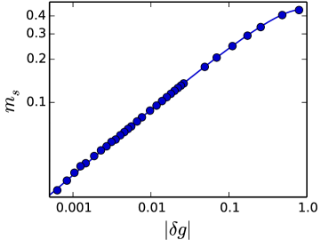
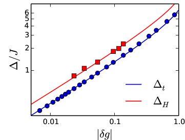
Here we present the results obtained by fitting the QMC data for the staggered magnetization, the triplon and Higgs excitation gaps, and the Néel temperature Qin et al. (2015, 2017) using the QFT expressions of Eqs. (22)-(25) and extract the numerical values of the remaining free parameters. The constants $g_{c}=4.83704$ and $c=2.365$ for the dimerized QAF on the double-cubic lattice are taken directly from QMC. Because the QFT framework presents a means of connecting sets of observables that are determined independently by QMC, we perform a complete fit to all data sets simultaneously. However, to do this in a reliable manner, the influence of different QMC points and of different datasets should be weighted according to their statistical reliability. Following the discussion in Sec. IIA, we weight the QMC datasets in the order $m_{s}>\Delta_{t}>\Delta_{H}>T_{N}$. As explained in more detail in Sec. IIIB, we give equal weight to all QMC data points in each set with $|\delta g|\leq 0.2$ and none to those at higher $|\delta g|$. The results are shown in Fig. 3.

These fits contain two adjustable parameters, which can be expressed as the mass proportionality factor $\gamma$ and the ratio $\alpha_{0}/(8\pi c^{3})$. It is important to note that the choice of the normalization point, $\Lambda_{0}$, is arbitrary, and affects directly the value of $\alpha_{0}$; because $\alpha_{0}\equiv\alpha_{\Lambda_{0}}$, any other choice of the normalization point, $\Lambda^{\prime}_{0}\neq\Lambda_{0}$, simply redefines $\alpha_{\Lambda^{\prime}_{0}}\equiv\alpha^{\prime}_{0}$. Here we make the explicit choice $\Lambda_{0}=0.915J$, based on the criterion $\Delta_{t}(\Lambda_{0})=\Lambda_{0}$, which proves to be convenient for the comparison with a bond-operator description (Sec. V). With this choice, the adjustable parameters are found to be

$$\alpha_{0}/(8\pi c^{3})=0.175,\ \ \gamma=3.95J,$$ (28)

and hence

$${\tilde{b}}_{1,2,3}=6.78,\ \ {\tilde{b}}_{4}=12.43.$$ (29)

Finally, an explicit relationship between the QFT order parameter, $\varphi_{c}$, and $m_{s}$ determined directly from QMC lies beyond the reach of QFT. We assume the relation

$$\varphi_{c} =\Upsilon m_{s},$$ (30)

and obtain $\Upsilon=0.65$ for the constant of proportionality. In Sec. V we justify the assumption of linearity and provide an analytic expression for $\Upsilon$ based on the bond-operator technique.

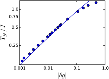
Figures 3(a), 3(b), and 3(c) show respectively our fits to $m_{s}$ (22), $\Delta_{t}$ (23) and $\Delta_{H}$ (24), and $T_{N}$ (25), which were made using the parameters of Eqs. (28) and (29). The logarithmic axes are chosen to highlight the multiplicative corrections as departures from the straight-line form of the mean-field exponents. Our major conclusion is the remarkable agreement between QMC and QFT, which demonstrates clearly that QFT, with a single set of parameters, is capable of providing a quantitative description, and hence a unification, of static and dynamic observables. This procedure also demonstrates once again, to high precision, the validity of the theoretical predictions of the O(3) QFT.

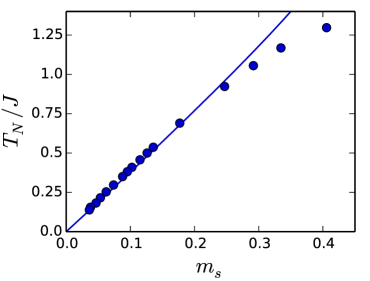
We comment that our fits in Fig. 3 are not identical to those of Ref. Qin et al. (2015). In the QMC study, the fits were found to be very insensitive to the values of the parameters ${\tilde{b}}_{i}$, which were set to $g_{c}$. In the QFT analysis, we gain both deeper insight into these parameters and a means of fixing them through constants to which the fits are more sensitive [Eq. (II.4)]. The ${\tilde{b}}_{i}$ values we obtain account for the minor quantitive differences between the fits, although we also did not implement an error-bar weighting as in Ref. Qin et al. (2015). The QFT analysis also affords extra insight into the linearity of $T_{N}$ and $m_{s}$, which is shown in Fig. 3(d). First observed numerically in Ref. Jin and Sandvik (2012), the almost exact linearity of the two parameters was studied in detail in Ref. Qin et al. (2015), where it was found that the two have the same logarithmic corrections; a scaling argument was formulated in support of this result, which has recently been observed again in a similar context Tan and Jiang (2017). From QFT it is clear immediately that $m_{s}$ (22) and $T_{N}$ (25) have multiplicative logarithmic corrections with the same exponent, illustrating again the unifying nature of the analysis. However, the arguments of the logarithms are not identical, due to the different cut-off energy scales, which are reflected in the different constants ${\tilde{b}}_{1}$ and ${\tilde{b}}_{4}$, and this is why the QFT fit in Fig. 3(d) is not in fact a completely straight line at large $|\delta g|$.

III.2 Quantum critical regime

A key question in the theory of quantum critical systems is to understand the width of the quantum critical regime [Fig. 1(b)], by which is meant the region of the phase diagram where the predicted quantum critical scaling forms [Eqs. (22)-(25)] remain applicable. The standard arguments of perturbative one-loop RG contain no such information, and cannot guarantee that the quantum critical regime is more than an asymptotic concept reached only when $|\delta g|\rightarrow 0$. Thus the width of this regime was referred to in Ref. Qin et al. (2015) as one of the nonuniversal constants of the system and it may be regarded as something of a surprise that quantum critical scaling was found in the QMC data over the rather broad range $|\delta g|\leq 0.2$. This estimate was obtained using the scaling forms of Eqs. (2) and (5), which make no explicit reference to the running coupling constant, $\alpha_{\Lambda}$. Hence one may ask whether this aspect of the QFT description provides additional insight into the width of the quantum critical regime.

Within the one-loop RG treatment, the QFT results remain accurate while the running coupling remains small, i.e. $\alpha_{\Lambda}/(8\pi c^{3})\ll 1$. This criterion is independent of the numerical analysis leading to $|\delta g|\leq 0.2$ and applies to all four of the observables we consider, which again demonstrates the unifying aspects of the QFT description. An explicit evaluation of Eq. (26) shows that $\alpha_{\Lambda}/(8\pi c^{3})=1$, the absolute upper bound on the applicability of one-loop RG as applied here, corresponds to $|\delta g|\approx 0.8$. Although one may debate the meaning of “small” relative to unity, it appears that the QMC estimate $|\delta g|\leq 0.2$ lies comfortably within the regime of validity of the QFT results.

One may, however, ask whether it is possible that quantum critical scaling could be obeyed for $|\delta g|\lesssim 1$. The agreement between the QFT form and the QMC data for both the staggered magnetization and the triplon gap [Figs. 3(a) and 3(b)], suggests that this may be the case. Here we comment again that such a level of agreement was not obtained in the initial analysis of the QMC data Qin et al. (2015), where the constant $b_{1}$ was imposed rather than deduced. Although the QFT fits shown in Fig. 3 were performed by using only the QMC data in the range $|\delta g|\leq 0.2$ (Sec. IIIA), this level of agreement demonstrates that the process we apply does not dictate the answer we obtain. This said, here we believe that the excellent agreement at the upper limit of the data range, $|\delta g|=0.8$, is probably accidental. There are no theoretical grounds on which to expect quantum critical scaling over such a broad parameter regime. The QFT analysis states that the description is not reliable by the time $\alpha_{\Lambda}/(8\pi c^{3})=1$. Further, the rather abrupt disagreement between QFT and QMC for $T_{N}(|\delta g|)$, which sets in beyond $|\delta g|\approx 0.1$ [Fig. 3(c)], suggests that the agreement is not global; this degree of mismatch cannot be ascribed to the lower accuracy of the QMC $T_{N}$ data compared to that of the $m_{s}$ data (Sec. IIA). Thus QFT tends to reinforce the QMC estimate that the width of the quantum critical regime is around $|\delta g|\leq 0.2$. Nevertheless, to the extent that the region beyond this limit is a crossover regime, detailed QMC and QFT studies of the double-cubic lattice would be an excellent means of probing crossover physics.

IV Results: Higgs decay width

The stability of the amplitude mode is a topic of crucial importance from the Standard Model to condensed matter and ultracold atoms. The broken symmetry of the ordered state, which establishes the massive Higgs mode, also ensures that Goldstone modes are ubiquitous, and with them a Higgs decay channel. Here we restrict our considerations to the line width arising due to Higgs decay processes in the 3D dimerized QAF. In the neutron scattering experiments on TlCuCl₃ Rüegg et al. (2008); Merchant et al. (2014), the amplitude mode was found, in contrast to the triplon modes, to have an intrinsic line width, which varied with temperature and proximity to the QCP.

Theoretically, the line width is extracted from a response function. For a system represented by a vector field, one may consider the response to vector or a scalar probe. In this sense, neutron scattering is a vector probe and the vector response function it provides is the dynamical spin-spin correlation function. The very recent dynamical QMC studies Qin et al. (2017); Lohöfer and Wessel (2017) applied advanced SAC methods to the imaginary-time Green functions obtained from SSE QMC to provide numerical data for both the vector and scalar response functions of the double-cubic QAF. Perhaps self-evidently, this analysis is restricted to the ordered phase, where spontaneous decay of the gapped triplet mode is possible; in the disordered phase, the spontaneous decay of triplons is forbidden by a lack of available phase space Scammell and Sushkov (2017a).

To discuss the decay of the Higgs mode at the upper critical dimension by QFT, we continue the analysis of the ordered phase begun in Sec. IIC3. When the vector field is reexpressed with an explicit separation of the amplitude component, i.e. $\vec{\varphi}=(\varphi_{c}+\sigma,\vec{\pi})$, the $\alpha\vec{\varphi}^{4}$ interaction term in Eq. (15) takes the form

$$\cal{V}_{\text{Int}} ={\textstyle\frac{1}{4}}\alpha(\sigma^{4}+\vec{\pi}^{4}+2\sigma^{2}\vec{\pi}^{2}+4\varphi_{c}\sigma^{3}+4\varphi_{c}\sigma\vec{\pi}^{2}).$$ (31)

The final term, $\alpha\varphi_{c}\sigma\vec{\pi}^{2}$ contains the leading-order coupling of the Higgs and Goldstone modes, which enables the decay of the former. We analyze this process by calculating the vector and scalar response functions within the one-loop QFT framework of Sec. II.3, using the parameters derived in Sec. III.

Figure 4: Diagrammatic expansion for the response function $\chi_{\sigma\sigma}$. The expansion is terminated at one-loop order, which corresponds to first order in $\alpha$. The double and dashed lines represent respectively the free propagation of the Higgs ($\sigma$) and Goldstone ($\vec{\pi}$) fields, obtained by setting $\vec{\varphi}=(\varphi_{c}+\sigma,\vec{\pi})$ in Eq. (6) and retaining terms to quadratic order in $\sigma$ and $\vec{\pi}$. Diagrams in the top line correspond to the quartic vertex terms, $\alpha\sigma^{4}$ and $\alpha\sigma^{2}\vec{\pi}^{2}$ in (31), and are clearly first-order in $\alpha$. Diagrams in the bottom line correspond to the cubic vertex terms $\alpha\varphi_{c}\sigma^{3}$ and $\alpha\varphi_{c}\sigma\vec{\pi}^{2}$. Although each diagram is a product of two $\alpha$ vertices, the fact that the coefficient $\alpha^{2}\varphi_{c}^{2}={\textstyle\frac{1}{2}}\alpha\Delta_{H}^{2}$, as shown in Eq. (20) of Sec. II.3, means that these terms remain first-order in $\alpha$. The evaluation of these diagrams is given by Eq. (34).

IV.1 Vector response function

The vector response function is defined as $\chi_{\varphi\varphi}(p)=\langle\vec{\varphi}(p)\,\vec{\varphi}(0)\rangle$. In terms of the Higgs and Goldstone components,

$$\chi_{\varphi\varphi}(p) =\langle\sigma(p)\sigma(0)\rangle+(N-1)\langle\pi(p)\pi(0)\rangle$$

$$=\chi_{\sigma\sigma}(p)+(N-1)\chi_{\pi\pi}(p).$$ (32)

In this form, the vector response is summed over all components and corresponds to an unpolarized probe. In this sense Eq. (IV.2) is equivalent to the quantity calculated in the QMC simulations, which are performed on finite-size lattices with unbroken spin-rotation symmetry. We note that there are no cross components of the Higgs field and the order parameter, i.e. $\chi_{\sigma\varphi_{c}}=0$.

Figure 5: Imaginary part of the vector response function, given by $-\chi^{\prime\prime}_{\sigma\sigma}(\omega)$, shown as a function of $\omega/\Delta_{H}$ at $\bm{p}=\bm{0}$ and normalized to its maximum value. The curves correspond to different values, $|\delta g|$, of the coupling ratio relative to the QCP.

We compute the response function at first order in $\alpha$. The Goldstone contribution, $\chi_{\pi\pi}(p)$, has no one-loop corrections, which is a direct consequence of the Goldstone theorem demonstrated explicitly in Sec. II.3, and hence

$$\chi_{\pi\pi}(p) =\frac{1}{p^{2}+i0}$$ (33)

where $i0$ in the denominator denotes the limiting imaginary part. The one-loop corrections to the Higgs component, represented in Fig. 4, are finite, and their real part was treated explicitly in Eq. (19). In all of the equations to follow, the Higgs gap, $\Delta_{H}$, represents the one-loop renormalized value given in Eq. (24) and it remains to evaluate the imaginary part of the one-loop corrections to the Higgs part of the response function. The first two loop diagrams on the right-hand side of Fig. 4 have purely real contributions, which are thus contained in the renormalized $\Delta_{H}$, and only the two terms on the lower line give imaginary contributions. These we label $\Pi_{H}(p)$ and $\Pi_{G}(p)$ to denote polarization loops with, respectively, with two Higgs and two Goldstone internal lines. Again their real parts have already been included in Eq. (19) and their imaginary parts, $\Pi^{\prime\prime}_{H}(p)$ and $\Pi^{\prime\prime}_{G}(p)$, give the result

$$\chi_{\sigma\sigma}(p) =\frac{1}{p^{2}-\Delta_{H}^{2}-{\textstyle\frac{1}{2}}i\alpha_{\Lambda}\Delta_{H}^{2}[9\Pi^{\prime\prime}_{H}(p)+\Pi^{\prime\prime}_{G}(p)]}$$ (34)

to this order. The polarization diagrams are given by standard loop-integral calculations Podolsky et al. (2011); Katan and Podolsky (2015) as

$$\Pi_{G}(p) =\frac{N-1}{8\pi^{2}c^{3}}\left[1+\ln\left(\frac{\Lambda_{0}^{2}}{p^{2}}\right)-i\pi\theta(p^{2})\right]\!,$$ (35)

$$\Pi_{H}(p) =\frac{1}{8\pi^{2}c^{3}}\left[1+\ln\left(\frac{\Lambda_{0}^{2}}{\Delta_{H}^{2}}\right)\right.$$ (36)

$$\;\;\;\;\;\;\;\;\;\;\;\;\;\;\;\;\left.-i\pi\frac{\sqrt{p^{2}-4\Delta_{H}^{2}}}{\sqrt{p^{2}}}\theta(p^{2}-4\Delta_{H}^{2})\right]\!,$$ (37)

where again $p^{2}=\omega^{2}-{\bm{p}}^{2}$ and $\theta$ is the Heaviside theta function.

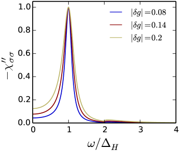
The spectral function for spin excitations is given by the imaginary part of the response function. To analyze the line width of the Higgs mode at its energy minimum, which occurs at spatial momentum $\bm{p}=\bm{0}$ (relative to the ordering wave vector, ${\bf Q}$), we show in Fig. 5 the quantity $-\chi_{\sigma\sigma}^{\prime\prime}(\omega,\bm{0})$. The spectral function has a Lorentzian shape, whose full-width at half-maximum height gives a decay width

$$\Gamma_{H}^{v}(|\delta g|) =\frac{\alpha_{\Lambda}}{8\pi c^{3}}\Delta_{H}(|\delta g|)$$

$$=\frac{\alpha_{0}\Delta_{H}(|\delta g|)}{8\pi c^{3}\left[1+\frac{(N+8)}{8\pi^{2}c^{3}}\alpha_{0}\ln(\sqrt{2}\Lambda_{0}/\Delta_{H})\right]}.$$ (38)

The first equality corresponds exactly to the width deduced from the Fermi golden rule in Ref. Kulik and Sushkov (2011) and the second uses the form of the running coupling constant deduced in Eq. (8); we stress that $\Delta_{H}$ contains further intrinsic dependence on $\alpha_{\Lambda}$. Physically, the dominant peak in Fig. 5 corresponds to the process where a Higgs mode decays spontaneously into two Goldstone modes, given by $\Pi^{\prime\prime}_{G}(\omega,\bm{0})$, while process of decay into two Higgs modes, $\Pi^{\prime\prime}_{H}(\omega,\bm{0})$, has a threshold at $\omega=2\Delta_{H}$ and does not to contribute to the line width, $\Gamma_{H}^{v}$.

Figure 6: Ratio $\Gamma_{H}^{v}/\Delta_{H}$ of the Higgs line width, as determined from the vector response function, to its gap, shown as a function of $|\delta g|$. The solid line is the QFT result obtained from Eq. (IV.1). The dashed line is the ratio extracted from QMC data by averaging over $|\delta g|$ and extrapolating in system size ($L\rightarrow\infty$) Qin et al. (2017). The points are obtained from the QMC data for systems of sizes $L=14$ and 16 at the different values of $|\delta g|$ for which simulations were performed.

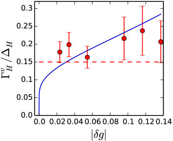
Clearly the Higgs decay width in the vector channel is determined completely by the fundamental parameters of the QFT. We use the best-fit parameters [(28) and (29)] for the double-cubic model to predict the Higgs line width (IV.1) as a function of $|\delta g|$ and show the results as the solid line in Fig. 6. For the width-to-gap ratio, we find a function with approximately linear dependence in the range $0.04<|\delta g|<0.2$, but which falls sharply to zero once $|\delta g|<0.02$. This latter behavior is dictated by the logarithmic terms in the running coupling constant and is in accord with the asymptotic freedom of the QFT at the QCP.

In Fig. 6 we show also the width-to-gap data deduced from the QMC simulations of Ref. Qin et al. (2017). It is apparent immediately that the statistical errors in the numerical results are large on the scale of the changes in this quantity. Because data obtained for different system sizes, $L$, showed a spread significantly greater than the spread resulting from the different $|\delta g|$ values, the data were analyzed by averaging over $|\delta g|$ and extrapolating the results to large $L$. The resulting estimate of a constant ratio, $\Gamma_{H}^{v}/\Delta_{H}=0.15$ (dashed line in Fig. 6), is equivalent to neglecting the logarithmic terms in Eq. (IV.1), and is consistent with experimental observations on TlCuCl₃ Rüegg et al. (2008); Merchant et al. (2014). The quantitative analysis made possible by QFT demonstrates that observing the dominant logarithmic corrections to the width-to-gap ratio requires values of $|\delta g|$ not currently accessible to numerics or experiment.

However, beyond the inaccessible regime $|\delta g|<0.02$, it is possible to perform an alternative analysis of the QMC data informed by the QFT results. The data points with error bars in Fig. 6 are obtained by considering the six $\delta g$ values individually. Instead of extrapolating in $L$, which would present very large errors, we retain only the two largest $L$ values ($L=14$ and 16) and show their error-weighted average. Despite the limitations of the numerical data, the matching trends of QFT and QMC illustrated in Fig. 6 suggest that future QMC studies with only factor-2 improvements in the error bars in $|\delta g|$ could indeed demonstrate the logarithmic form of the Higgs decay width obtained from the vector response function.

IV.2 Scalar response function

Turning now to the scalar response function, $\chi_{\varphi^{2}\varphi^{2}}(p)=\langle\vec{\varphi}^{2}(p)\,\vec{\varphi}^{2}(0)\rangle$, we use again the substitution $\vec{\varphi}=(\varphi_{c}+\sigma,\vec{\pi})$ to effect a decomposition into Higgs and Goldstone components,

$$\chi_{\varphi^{2}\varphi^{2}}(p) =4\varphi_{c}^{2}\chi_{\sigma\sigma}(p)+4\varphi_{c}[\chi_{\sigma\pi^{2}}(p)+\chi_{\sigma\sigma^{2}}(p)]$$

$$\;\;\;\;+\chi_{\sigma^{2}\sigma^{2}}(p)+2\chi_{\sigma^{2}\pi^{2}}(p)+\chi_{\pi^{2}\pi^{2}}(p).$$ (39)

Assisted by our results for the vector response (Sec. IVA), we consider only the Higgs contributions to $\chi_{\varphi^{2}\varphi^{2}}$ at order $\alpha$; an alternative derivation may be found in Refs. Podolsky et al. (2011); Katan and Podolsky (2015). We note first that

$$\chi_{\pi^{2}\pi^{2}}(p) =\langle\pi^{2}(p)\pi^{2}(0)\rangle=\Pi_{G}(p)$$

$$\chi_{\sigma^{2}\sigma^{2}}(p) =\langle\sigma^{2}(p)\sigma^{2}(0)\rangle=\Pi_{H}(p)$$

are simply the Goldstone and Higgs polarization loops represented graphically on the bottom line of Fig. 4, which are given respectively by Eqs. (35) and (36).

For a first-order expansion of the other terms in $\chi_{\varphi^{2}\varphi^{2}}$, it is necessary to consider the form of coupling terms between the different fields allowed by the interaction, as specified in Eq. (31). In the case of the second term in Eq. (IV.2), we obtain

$$4\varphi_{c}(\chi_{\sigma\pi^{2}}+\chi_{\sigma\sigma^{2}}) =4\varphi_{c}(\langle\sigma\pi^{2}\rangle+\langle\sigma\sigma^{2}\rangle+\langle\sigma[\alpha\varphi_{c}\sigma\pi^{2}]\pi^{2}\rangle$$

$$\;\;\;\;\;\;\;\;\;\;\;\;\;\;\;\;+\langle\sigma[\alpha\varphi_{c}\sigma\sigma^{2}]\sigma^{2}\rangle)$$

$$=4\alpha\varphi^{2}_{c}(\langle\sigma\sigma\rangle\langle\pi^{2}\pi^{2}\rangle+3\langle\sigma\sigma\rangle\langle\sigma^{2}\sigma^{2}\rangle)$$

$$=4\alpha\varphi^{2}_{c}\chi_{\sigma\sigma}(\Pi_{G}+3\Pi_{H}).$$ (40)

Here the terms $\langle\sigma\pi^{2}\rangle=\langle\sigma\sigma^{2}\rangle=0$ because there is no zeroth-order coupling of these fields. For the two terms in the second line, the insertions $[\alpha\varphi_{c}\sigma\pi^{2}]$ and $[\alpha\varphi_{c}\sigma\sigma^{2}]$ show the only terms in Eq. (31) coupling the fields at first order in the perturbative expansion. By the same reasoning,

$$\chi_{\sigma^{2}\sigma^{2}} = \langle\sigma^{2}\sigma^{2}\rangle+(\alpha\varphi_{c})^{2}\langle\sigma^{2}[\sigma^{2}\sigma\sigma\sigma^{2}]\sigma^{2}\rangle$$ (41)

$$= \Pi_{H}+9(\alpha\varphi_{c})^{2}\Pi_{H}\chi_{\sigma\sigma}\Pi_{H},$$

$$\chi_{\pi^{2}\pi^{2}} = \langle\pi^{2}\pi^{2}\rangle+(\alpha\varphi_{c})^{2}\langle\pi^{2}[\pi^{2}\sigma\sigma\pi^{2}]\pi^{2}\rangle$$ (42)

$$= \Pi_{G}+(\alpha\varphi_{c})^{2}\Pi_{G}\chi_{\sigma\sigma}\Pi_{G},$$

$$2\chi_{\sigma^{2}\pi^{2}} = 2(\alpha\varphi_{c})^{2}\langle\sigma^{2}[\sigma^{2}\sigma\sigma\pi^{2}]\pi^{2}\rangle$$ (43)

$$= 3(\alpha\varphi_{c})^{2}\Pi_{H}\chi_{\sigma\sigma}\Pi_{G},$$

and hence by summing all contributions in Eq. (IV.2) we obtain

$$\chi_{\varphi^{2}\varphi^{2}} = 4\alpha\varphi^{2}_{c}\chi_{\sigma\sigma}[1+\alpha(\Pi_{G}+3\Pi_{H})$$

$$\;\;+{\textstyle\frac{1}{4}}\alpha^{2}(\Pi_{G}^{2}+9\Pi_{H}^{2}+6\Pi_{G}\Pi_{H})]+\Pi_{G}+\Pi_{H}.$$

It is clear from the perturbative procedure that the divergent part of the scalar response function is linearly proportional to the vector response, $\chi_{\sigma\sigma}$ [Eq. (34) and Fig. 4], and hence will share its pole structure. We note again that the terms $\Pi_{G}$ and $\Pi_{H}$ appearing in Eq. (IV.2) have both real and imaginary parts, the first of which are responsible for the renormalization of the quantities $\varphi_{c}$ and $\Delta_{H}$, leading to the logarithmic corrections discussed in Sec. II.3. Again we absorb these real parts into $\varphi_{c}$ and $\Delta_{H}$, showing only the imaginary parts, $\Pi_{G}^{\prime\prime}$ and $\Pi_{H}^{\prime\prime}$, which do not influence the renormalization. The final expression for the scalar response function is then

$$\chi_{\varphi^{2}\varphi^{2}}(p) =\frac{2\Delta_{H}^{2}}{\alpha_{\Lambda}}\frac{\{1+\frac{1}{2}\alpha_{\Lambda}[\Pi^{\prime\prime}_{G}(p)+3\Pi^{\prime\prime}_{H}(p)]\}^{2}}{p^{2}-\Delta_{H}^{2}-\frac{i}{2}\alpha_{\Lambda}\Delta_{H}^{2}\left[\Pi^{\prime\prime}_{G}(p)+9\Pi^{\prime\prime}_{H}(p)\right]}$$

$$\;\;\;\;\;\;\;\;+\Pi^{\prime\prime}_{G}(p)+\Pi^{\prime\prime}_{H}(p),$$ (45)

and the imaginary part of this quantity, which is the zone-center dimer-dimer spectral function of the double-cubic model, is shown as a function of the frequency $\omega$ at relative spatial wave vector ${\bm{p}}={\bm{0}}$.

Figure 7: Imaginary part of the scalar response function, $-\chi^{\prime\prime}_{\varphi^{2}\varphi^{2}}(\omega)$, shown as a function of $\omega/\Delta_{H}$ at $\bm{p}=\bm{0}$ and normalized to its maximum value. The curves are evaluated from Eq. (IV.2) and correspond to different values, $|\delta g|$, of the coupling ratio relative to the QCP. Dashed lines show the results obtained from Eq. (IV.2) but neglecting the two-Higgs contribution [Eq. (36)].

Several comments are in order concerning this result. First, the pole structure of the scalar response function is indeed identical to the vector response. The only difference to the spectral function is a prefactor arising from the imaginary part of the first term of Eq. (IV.2). Second, there are non-resonant pole contributions to $\chi_{\varphi^{2}\varphi^{2}}(\omega)$, which are contained in the lower line of Eq. (IV.2). In the limit of large four-momentum, $p^{2}\gg\Delta_{H}^{2}$, these terms are dominant and the background scattering they contribute can be shown from Eqs. (35) and (36) to have the asymptotic form

$$\Pi^{\prime\prime}_{G}(p)+\Pi^{\prime\prime}_{H}(p^{2}\gg\Delta_{H}^{2}) \longrightarrow\frac{3}{8\pi}.$$ (46)

Setting $p=(\omega,\bm{0})$ in Eq. (46) accounts for the spectral weight of the high-$\omega$ tail in Fig. 7.

Third, the phase of the prefactor and non-resonant pole terms contribute to a destructive interference in the emission channel of two low-energy Goldstone modes. This interference suppresses the imaginary part of the scalar response, resulting in the power-law form $\chi_{\varphi^{2}\varphi^{2}}(p)\propto p^{4}$ as $p\rightarrow 0$ in the present 3+1D problem, which is a statement of the Adler theorem. To show this explicitly, we reexpress the imaginary part of Eq. (IV.2) in the form, valid for $p^{2}<4\Delta_{H}^{2}$,

$$\chi^{\prime\prime}_{\varphi^{2}\varphi^{2}} =\frac{-p^{4}\Pi^{\prime\prime}_{G}(p)}{(p^{2}-\Delta_{H}^{2})^{2}+[\frac{1}{2}\alpha_{\Lambda}\Delta_{H}^{2}\Pi^{\prime\prime}_{G}(p)]^{2}}.$$ (47)

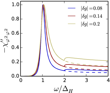
Here we have neglected the $\Pi_{H}(p)$ term, which makes no contribution to the imaginary part for $p^{2}<4\Delta_{H}^{2}$. The line shape of the scalar response function at ${\bm{p}}={\bm{0}}$, shown in Fig. 7, is that of a Fano resonance, but with additional interference contributions that result in an $\omega^{4}$ form of the infrared tail Podolsky et al. (2011). This asymmetric shape compares well with recent QMC results Qin et al. (2017); Lohöfer and Wessel (2017). However, our inclusion of the logarithmic corrections prevents any collapse of either the scalar or the vector response curves to a single ‘universal’ form, as suggested by some of the QMC data.

Figure 8: Ratio $\Gamma_{H}^{s}/\Delta_{H}$ of the Higgs line width, as determined from the scalar response function, to its gap, shown as a function of $|\delta g|$. The solid line is the QFT result obtained from Eqs. (IV.2) and (IV.1). The dashed line is the ratio extracted from QMC data by averaging over $|\delta g|$ and extrapolating in system size ($L\rightarrow\infty$) Qin et al. (2017). The points are obtained from the QMC data for systems of sizes $L=14$ and 16 at the different values of $|\delta g|$ for which simulations were performed.

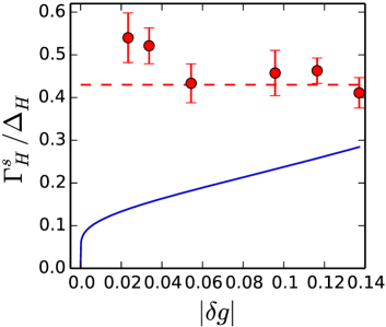
Finally, we comment on the Higgs decay width extracted from the scalar response function of Eq. (IV.2). While the asymmetric, non-Lorenzian shape of the dimer-dimer spectral function (Fig. 7) prevents us from obtaining a direct analytic expression, to a good approximation the line width is still the value determined directly from the imaginary part of the denominator in Eq. (IV.2), which is identical to the result for the vector response (34). Thus we obtain (IV.1) $\Gamma^{s}_{H}\approx\Gamma^{v}_{H}=\alpha_{\Lambda}\Delta_{H}/8\pi c^{3}$.

In Fig. 8 we plot the ratio $\Gamma_{H}^{s}/\Delta_{H}$, which for QFT is identical to the curve in Fig. 6, for comparison with the results obtained from the QMC simulations of Ref. Qin et al. (2017). Following the same procedure of averaging over $|\delta g|$ and extrapolating to large $L$ led to an anticipated constant ratio $\Gamma_{H}^{s}/\Delta_{H}=0.43$, as shown by the dashed line. We show again the alternative analysis of retaining the individual $|\delta g|$ data and considering only the largest accessible values of $L$. In this case the QFT and QMC results differ very significantly, not only in magnitude but also in apparent functional form. Such a discrepancy cannot be ascribed solely to statistical errors in the QMC data and make clear that some systematic factors are also at work; one may speculate for example that the error bars on the imaginary-time QMC data have a particularly strong broadening effect in the SAC procedure for the scalar response function, in a way that does not affect the vector response. Further QMC and analytic continuation studies, including with simulated data obeying different error criteria, may be used to test such a hypothesis for different spectral functions.

In summary, the extraction of the Higgs line width lies at the limits of current QMC data. Their accuracy is not yet sufficient to discern logarithmic corrections in this quantity from the vector response function (Fig. 6), while only the qualitative nature of the scalar response function is accessible (Fig. 7). There has to date been no theoretical expectation with which to compare these results, and thus the present QFT analysis provides an essential quantitative benchmark. It is certainly desirable for future numerical studies to focus on the logarithmic dependence of the Higgs line width, which ultimately is expected because the theory becomes asymptotically free at the QCP.

V Microscopic derivation of QFT parameters

The Lagrangian field theory (6) is a low-energy approximation to the full physics of the Hamiltonian (1). Although we have shown that Eq. (6) delivers an excellent description of the unbiased numerical data obtained by QMC simulations, the parameters we have used in making this comparison are fitted, and hence rank as phenomenological, i.e. an explicit connection to the “fundamental” parameters, $J$ and $J^{\prime}$ of the underlying spin model (1) is lost. Here we employ a microscopic description, the bond-operator framework, to demonstrate the bridging of this gap between QFT and the spin Hamiltonian. Specifically, we will derive expressions for $\gamma$, $c$, and $g_{c}$ directly in terms of $J$ and $J^{\prime}$ and provide an analytic justification for the linear relationship between $\varphi_{c}$ of QFT and $m_{s}$ of the spin Hamiltonian. However, this analytic treatment does not provide results for the arbitrary normalization points $\alpha_{0}$ and $\Lambda_{0}$ of the QFT.

V.1 Triplon gap, velocity, and the QCP

The bond-operator representation Sachdev and Bhatt (1990) is an identity for spin-$1/2$ operators that is particularly well adapted to the analysis of dimerized quantum magnets Gopalan et al. (1994). When all the spins of the system reside on one dominant bond, as in Eq. (1) when $g\gg g_{c}$, it is logical to express the spin degrees of freedom as

$${\bm{S}}^{l,r}_{i} ={\textstyle\frac{1}{2}}(\pm s_{i}^{{\dagger}}t_{i,\alpha}\pm t_{i,\alpha}^{{\dagger}}s_{i}-i\epsilon_{\alpha,\beta,\gamma}t_{i,\beta}^{\dagger}t_{i,\gamma})$$ (48)

where $s_{i}^{{\dagger}}$ is an operator creating the singlet state of the two spins on bond $i$ and $t_{i,\alpha}^{{\dagger}}$ creates one of the three triplet states. These singlet and triplet states have bosonic commutation relations, but from the nature of the underlying spin degrees of freedom are nevertheless mutually exclusive (i.e.  they are hard-core bosons Sachdev and Bhatt (1990)). When a system is strongly dimerized, its ground state may be treated as a condensate of bond singlets whose coherence is mediated by the hopping of (well gapped) triplet excitations, and hence it is an excellent approximation to replace the operators $s_{i}^{{\dagger}}$ and $s_{i}$ by their condensate expectation value, $\langle s\rangle=\bar{s}$.

By applying the transformation of Eq. (48) to the QAF on the double-cubic lattice (1) and performing standard Fourier and Bogoliubov transformations, we derive two mean-field equations whose self-consistent solution provides a quantitative description of the system for any coupling ratio, $g$. Full details of this procedure are provided in the Appendix. Although the two mean-field bond-operator parameters are in principle a function of $g$, we obtain a singlet condensation $\bar{s}=0.97$ for all values of $g$ in a broad region around the QCP. This includes the ordered phase, considered in the bond-operator formulation in Refs. Matsumoto et al. and Rüegg et al. (2008), where the physical understanding of the magnetic state is small degree of antiferromagnetic order superposed on strongly fluctuating singlet correlations. For the present purposes, we focus on the bond-operator expression for the gap to triplon excitations in the quantum disordered phase, $\Delta_{\text{BO}}=\left({\textstyle\frac{1}{4}}J^{\prime}-\mu\right)[1-3d]^{1/2}$ [Eq. (67)], which we distinguish from $\Delta_{t}$ [Eq. (23)] obtained in QFT. Here $\mu$ is the other mean-field parameter, which corresponds to a triplon chemical potential, while $d$ is an average quantity depending linearly on $J$ and $\bar{s}^{2}$ as shown in the Appendix.

Having found two expressions for the triplon gap, one of which is given directly in terms of the fundamental parameters $J$ and $J^{\prime}$, we can estimate the coefficient $\gamma$ in the QFT gap [Eq. (23)]. We equate the two gaps at the normalization point, $\Lambda_{0}$, to obtain the approximation

$$\gamma^{2}=\frac{\Delta^{2}_{\text{BO}}(\Lambda_{0})}{|\delta g(\Lambda_{0})|}.$$ (49)

Having chosen the normalization point $\Lambda_{0}=0.915J$ on the basis of the criterion $\Delta_{t}(\Lambda_{0})=\Lambda_{0}$, we find that $|\delta g(\Lambda_{0})|\approx 0.056$ and thus obtain the estimate $\gamma=3.88J$. This compares rather well with the value $\gamma=3.95J$ obtained in Eq. (28), demonstrating that the phenomenological parameters required to fit the QMC data do indeed have a direct microscopic basis.

The QCP in the bond-operator approach can be found by setting $\Delta_{\text{BO}}=0$, which yields the value $g_{c}=4.96$, in good agreement with the numerically exact result, $g_{c}=4.83704$ Qin et al. (2015). We also estimate the spin-wave velocity at the QCP from

$$c=\lim_{{\bm{q}}\rightarrow{\bm{Q}}}\frac{\Omega_{\bm{q}}(g_{c})}{|{\bm{q}}-{\bm{Q}}|}=2.28,$$ (50)

where $\Omega_{\bm{q}}(g)$ is the bond-operator triplon spectrum derived in the Appendix and $\bm{Q}$, the antiferromagnetic point in the Brillouin zone, is where the gap closes at $g_{c}$. Again we obtain good agreement with the QMC result, $c=2.365$, demonstrating the quantitative accuracy of the bond-operator description.

V.2 Relationship of $m_{s}$ and $\varphi_{c}$

As noted in Sec. IIIA, QFT cannot specify the staggered magnetization, $m_{s}$, directly, providing instead the order parameter, $\varphi_{c}$. To derive the relation between $m_{s}$ and $\varphi_{c}$, we consider the triplon bond operator, which we express as the vector $\vec{t}$, to find the constant of proportionality, $Z$, in the equation

$$\vec{\varphi}={\textstyle\frac{1}{2}}Z^{-1}(\vec{t}\ ^{\dagger}+\vec{t})$$ (51)

relating it to the vector field $\vec{\varphi}$. Working in real space,

$$\varphi(x) =\sum_{\bm{k}}\frac{1}{\sqrt{2\Omega_{\bm{k}}}}\left[\beta_{\bm{k}}e^{ikx}+\beta_{\bm{k}}^{\dagger}e^{-ikx}\right]\!,$$ (52)

$$t(x) =\sum_{\bm{k}}\left[u_{\bm{k}}\beta_{\bm{k}}-v_{-{\bm{k}}}\beta_{-{\bm{k}}}^{\dagger}\right]e^{ikx},$$ (53)

$$\approx\sum_{\bm{k}}\sqrt{\frac{A_{\bm{k}}}{2\Omega_{\bm{k}}}}\left[\beta_{\bm{k}}e^{ikx}+\beta_{\bm{k}}^{\dagger}e^{-ikx}\right]\!,$$ (54)

where $\beta_{k}$ are the Bogoliubov operators diagonalizing the triplon Hamiltonian, $u_{{\bm{k}}}$ and $v_{{\bm{k}}}$ are the corresponding coefficients, defined in Eq. (62), and $A_{\bm{k}}$ (63) are the diagonal components of the triplon matrix. In the vicinity of the QCP, the dominant contributions to the wave-vector sums are from low-energy excitations with ${\bm{k}}$ of order ${\bm{Q}}$, allowing the approximation

$$Z=\frac{1}{\sqrt{A_{\bm{Q}}}}.$$ (55)

The staggered magnetization of the QAF is

$$m_{s}^{z} =\frac{1}{N}\langle S^{lz}-S^{rz}\rangle,$$ (56)

where $S^{zl,zr}=\sum_{i}^{N^{\prime}}S^{zl,zr}_{i}$ with $N^{\prime}=N/2$ the number of sites on each sublattice, whence

$$m_{s}^{z} =\frac{1}{2N}\left\langle\sum_{i\in A}^{N^{\prime}}(s_{i}^{{\dagger}}t_{i,z}+t_{i,z}^{{\dagger}}s_{i})+\sum_{i\in B}^{N^{\prime}}(s_{i}^{{\dagger}}t_{i,z}+t_{i,z}^{{\dagger}}s_{i})\right\rangle$$

$$={\textstyle\frac{1}{2}}{\bar{s}}\langle t_{z}+t_{z}^{\dagger}\rangle=\bar{s}Z\langle\varphi_{z}\rangle$$ (57)

and thus, because $\langle\varphi_{z}\rangle=\varphi_{c}$,

$$\Upsilon =\frac{\varphi_{c}}{m_{s}^{z}}\;=\;\sqrt{\frac{1}{\bar{s}^{2}A_{{\bm{Q}}}}}\;=\;0.62.$$ (58)

Once again we obtain a good microscopic account of the value $\Upsilon=0.65$ deduced in Fig. 3(b) by applying the QFT fitting framework to the QMC data.

VI Discussion

In summary, we have considered the critical properties of 3D quantum antiferromagnets as an example of a physical system at the upper critical dimension. The ability to obtain unbiased numerical data from QMC, of a precision high enough to verify multiplicative logarithmic corrections around the QCP in both static and dynamic observables, is an achievement at the frontier of current computational capabilities. By interpreting these data within the framework of an effective QFT, we obtain (i) unified physical insight into the connection between the static and dynamical properties of critical systems, (ii) a thorough test of perturbative O(3) QFT, and (iii) a valuable guide for the understanding of numerical and experimental studies probing quantum critical phenomena in a range of physical systems.

At a pragmatic level, the present work offers a means for direct comparison between QMC and QFT. QMC data are obtained directly from the spin ($J$–$J^{\prime}$) Hamiltonian (1), whereas QFT results are derived in terms of the quasiparticles of a low-energy effective Lagrangian for long-wavelength fields (6). The excellent overall agreement demonstrates clearly the ability of the low-energy theory to capture all of the relevant physics in the vicinity of the QCP, and a quantitative description of the observables of the system allows the number of unknown parameters in the QFT to be reduced significantly. Once these fitting parameters are obtained, the QFT becomes predictive, which we demonstrate by calculating the vector and scalar response functions with an accuracy not currently achievable by QMC.

It is well known from general QFT that the dimensionality and symmetry properties of a system determine the critical indices of its observables uniquely in the regime around the QCP. Previous numerical and experimental tests of universality have therefore focused on individual critical indices. In the present QFT analysis, we go beyond the asymptotic scaling behavior to provide a quantitative description of the observables and thus to investigate how they are connected. The crucial physical insight underlying unification of the thermodynamic and dynamic quantities is that the logarithmic corrections to their scaling specified in Eqs. (2)-(5) may all be understood in terms of the running coupling constant (8) between the quasiparticles of the QFT.

Here we have focused primarily on the zero-temperature behavior of the system, as contained in the order parameter, gaps, and decay widths. Finite temperatures introduce thermal as well as quantum fluctuations and produce many exotic phenomena not present at zero temperature Sachdev (1997, 1999, 2011); Vojta (2003). In particular, thermal fluctuations are responsible for the crossover into regions of the phase diagram marked as ‘quantum critical’ in Fig. 1(a), where they interfere qualitatively with quantum effects, and are dominant in the region marked as ‘classical critical.’ In these regimes, the observables of the system show different types of characteristic scaling behavior, to the point where the results of classical statistical mechanics are recovered. In this context it is crucial to remark that the finite-temperature behavior of the physical observables in QFT is completely determined by the results we present here (Sec. II.3 and Ref. Scammell and Sushkov (2015)), i.e. an analysis of finite-temperature properties would require no new fitting parameters. Because QMC is actually easier at finite temperatures, where no extrapolation is required in the corresponding system dimension, a quantitative investigation of static and dynamical properties across the full phase diagram by combining QFT and QMC is definitely feasible.

Qualitatively, finite temperatures also generate additional scattering channels for quasiparticles, which are sometimes modelled as a heat bath. Among the physical implications of heat-bath scattering is the possibility that triplons in the disordered phase, which have infinite lifetimes at zero temperature, can acquire a substantial decay width. This situation has been investigated experimentally in TlCuCl₃ Merchant et al. (2014) and discussed analytically in Refs. Scammell and Sushkov (2017a); Fidrysiak and Spałek (2017) for the quantum antiferromagnet and Ref. Nagao and Danshita for the Bose gas. A corresponding numerical (QMC) study of triplon decay at finite temperatures has yet to be performed.

A key additional direction for the extension of the present analysis is to include the effects of an applied magnetic field, which provides an explicit breaking of the spin symmetry. Early theoretical Nikuni et al. (2000) and experimental Rüegg et al. (2003) studies of the quantum antiferromagnet in the presence of a magnetic field investigated the phenomenology of magnon Bose-Einstein condensation, and suitably modified QFT descriptions have been used to discuss the associated critical scaling behavior Fisher (1989); Sachdev (1997); Scammell and Sushkov (2017b). Early QMC studies were also made of the magnon Bose-Einstein condensation scenario in 3D Wessel et al. (2001); Nohadani et al. (2004, 2005), while some exotic theoretical predictions for quasi-1D systems Orignac et al. (2007) remain to be tested numerically. Once again, a QFT description of the critical observables can be obtained from the present work without the need for additional fitting parameters. Indeed, in a recent study of the 3D case, some of us Scammell and Sushkov (2017b) predicted that two new critical indices emerge in the presence of an applied magnetic field and that logarithmic corrections are an important feature of the scaling behavior. To date there exists no related QMC analysis of a precision suitable for a comparative test.

Finally, we anticipate that our results and techniques will serve as a helpful guide for future experimental and numerical studies of quantum critical phenomena. The reality of the situation is that research of the frontier of what is currently possible is always struggling for adequate data, by which is meant both enough data and sufficiently accurate data. The consequences of our results for numerical analysis include improved interpretation and understanding of critical regimes, the ability to relate datasets to reduce statistical errors, and qualitative guidance in previously unexplored but feasible directions. The additional consequences for experiment include the fact that all measurements in condensed matter and ultracold atomic condensates are made at finite temperature, and thus a systematic means of understanding the quantum limit is indispensible.

Appendix A Bond-Operator Representation

Here we provide details of the bond-operator technique and its application to the spin Hamiltonian of the 3D dimerized QAF (1). As stated in Sec. V, the bond-operator representation of spins ${\bm{S}}^{l,r}_{i}$ [Eq. (48)] is particularly appropriate for a dimerized QAF. The most important point about the identity (48) is that it must satisfy the SU(2) spin algebra,

$$[S_{\alpha}^{m},S_{\beta}^{m}] =i\epsilon_{\alpha\beta\gamma}S_{\gamma}^{m},\;\;\;\;[S_{\alpha}^{l},S_{\beta}^{r}]=0,$$

which in fact sets two conditions on the bond operators $s_{i}^{\dagger}$ and $t_{i,\alpha}^{\dagger}$. One is that they must have bosonic commutation relations and the other that the space of physical states on any dimer bond constrains their total number to satisfy $s_{i}^{\dagger}s_{i}+t_{i,\alpha}^{\dagger}t_{i,\alpha}=1$. However, satisfying this constraint on every dimer bond, $i$, leads to a problem that cannot be treated analytically and is extremely demanding numerically, but it has been shown Matsumoto et al. ; Rüegg et al. (2008); Merchant et al. (2014) for the 3D QAF that satisfying the constraint only on average leads to quantitatively accurate results. This we effect using a Lagrange multiplier, $\mu$, that is the same on all sites Sachdev and Bhatt (1990).

By applying the transformation of Eq. (48), the dimer-bond part of Hamiltonian (1) becomes

$$H_{0}=J^{\prime}\sum_{i}-{\textstyle\frac{3}{4}}s_{i}^{{\dagger}}s_{i}+{\textstyle\frac{1}{4}}t_{i,\alpha}^{{\dagger}}t_{i,\alpha}-\mu(s_{i}^{\dagger}s_{i}+t_{i,\alpha}^{\dagger}t_{i,\alpha}-1).$$ (59)

The inter-dimer part contributes terms of higher order in the operators $s_{i}$ and $t_{i,\alpha}$ and, by retaining only those at quadratic order in $t_{i,\alpha}$, i.e. by neglecting triplon interactions, we obtain

$$H_{2} ={\textstyle\frac{1}{2}}J\sum_{<i,j>}s_{i}^{{\dagger}}s_{j}^{\dagger}t_{i,\alpha}t_{j,\alpha}+s_{i}^{{\dagger}}s_{j}t_{i,\alpha}t_{j,\alpha}^{\dagger}+\text{H.c.}$$ (60)

This we treat in the approximation of complete Bose condensation of singlets, i.e. we neglect singlet fluctuations and replace $s_{i}^{\dagger}$ and $s_{i}$ by the constant $\bar{s}$.

The quadratic Hamiltonian $H_{0}+H_{2}$ is expressed in reciprocal space using $t_{i,\alpha}^{\dagger}=\frac{1}{\sqrt{N^{\prime}}}\sum_{\bm{k}}t_{\bm{k},\alpha}e^{-i\bm{k}\cdot\bm{R}_{i}}$, where $N^{\prime}=N/2$ is the number of dimers, and diagonalized by a Bogoliubov transformations. The dynamical terms in the resulting Hamiltonian are

$$\bar{H}_{2} =\sum_{\bm{k}}A_{\bm{k}}t_{\bm{k},\alpha}^{\dagger}t_{\bm{k},\alpha}+{\textstyle\frac{1}{2}}B_{\bm{k}}[t_{\bm{k},\alpha}^{\dagger}t_{-\bm{k},\alpha}^{\dagger}+\text{H.c.}]$$

$$=\sum_{\bm{k}}\Omega_{\bm{k}}\beta_{\bm{k},\alpha}^{\dagger}\beta_{\bm{k},\alpha},$$ (61)

where

$$t_{\bm{k},\alpha}^{\dagger} =u_{\bm{k}}\beta_{\bm{k},\alpha}^{\dagger}-v_{\bm{k}}\beta_{-\bm{k},\alpha}, \Omega_{\bm{k}}=\sqrt{A_{\bm{k}}^{2}-B_{\bm{k}}^{2}}$$

$$u_{\bm{k}}^{2},v_{\bm{k}}^{2} =\pm\frac{1}{2}+\frac{A_{\bm{k}}}{2\Omega_{\bm{k}}}, u_{\bm{k}}v_{\bm{k}}=\frac{B_{\bm{k}}}{2\Omega_{\bm{k}}}.$$ (62)

The coefficients $A_{\bm{k}}$ and $B_{\bm{k}}$ depend on the lattice geometry and for the double-cubic model are

$$A_{\bm{k}} ={\textstyle\frac{1}{4}}J^{\prime}-\mu+J\bar{s}^{2}\,[\cos k_{x}+\cos k_{y}+\cos k_{z}]$$

$$B_{\bm{k}} =J\bar{s}^{2}\,[\cos k_{x}+\cos k_{y}+\cos k_{z}].$$ (63)

To obtain an expression for the triplon spectrum and hence the gap, it is necessary to deduce the mean-field parameters $\mu$ and $\bar{s}$, which are obtained from the saddle-point conditions

$$\left\langle\frac{\partial H_{MF}}{\partial\mu}\right\rangle =0, \left\langle\frac{\partial H_{MF}}{\partial\bar{s}}\right\rangle=0,$$ (64)

in which $H_{MF}=\bar{H}_{0}+\bar{H}_{2}$ denotes both the constant and dynamical parts of the quadratic mean-field Hamiltonian. It is convenient Gopalan et al. (1994) to introduce the dimensionless parameter

$$d=\frac{2J\bar{s}^{2}}{{\textstyle\frac{1}{4}}J^{\prime}-\mu},$$ (65)

in terms of which the self-consistent mean-field equations are

$$\bar{s}^{2} =\frac{5}{2}-\frac{3}{2N^{\prime}}\sum_{\bm{k}}\frac{1+d\gamma_{\bm{k}}}{\sqrt{1+2d\gamma_{\bm{k}}}},$$

$$\mu =-\frac{3J^{\prime}}{4}+\frac{3J}{N^{\prime}}\sum_{\bm{k}}\frac{\gamma_{\bm{k}}}{\sqrt{1+2d\gamma_{\bm{k}}}},$$ (66)

with

$$d =\frac{J}{J^{\prime}}\left(5-\frac{3}{N^{\prime}}\sum_{\bm{k}}\frac{1}{\sqrt{1+2d\gamma_{\bm{k}}}}\right)\!,$$

$$\gamma_{\bm{k}} ={\textstyle\frac{1}{2}}[\cos k_{x}+\cos k_{y}+\cos k_{z}].$$

The triplon spectrum may now be expressed as

$$\Omega_{\bm{k}} =\left({\textstyle\frac{1}{4}}J^{\prime}-\mu\right)[1+2d\gamma_{\bm{k}}]^{1/2}$$

and the gap as

$$\Delta_{\text{BO}} =\left({\textstyle\frac{1}{4}}J^{\prime}-\mu\right)[1-3d]^{1/2}.$$ (67)

This expression for $\Delta_{\text{BO}}$ was used to evaluate $\gamma$ in Eq. (49) and to derive the bond-operator value of the QCP, $J^{\prime}/J=g_{c}=4.96$; at values of $g$ around $g_{c}$, we obtain the result $\bar{s}=0.97$, which was used in Eq. (58) to evaluate $\Upsilon$.

References

- Zinn-Justin (2002) J. Zinn-Justin, Quantum Field Theory and Critical Phenomena, International series of monographs on physics (Clarendon Press, 2002).
- Sachdev (2011) S. Sachdev, Quantum Phase Transitions (Cambridge University Press, 2011).
- Kenna and Lang (1993) R. Kenna and C. Lang, Nuclear Physics B 393, 461 (1993).
- Kenna and Lang (1994) R. Kenna and C. B. Lang, Nuclear Physics B 411, 340 (1994).
- Wegner and Riedel (1973) F. J. Wegner and E. K. Riedel, Phys. Rev. B 7, 248 (1973).
- Domb et al. (1976) C. Domb, M. Green, and J. Lebowitz, Phase transitions and critical phenomena, Phase Transitions and Critical Phenomena (Academic Press, 1976).
- Hara and Tasaki (1987) T. Hara and H. Tasaki, Journal of Statistical Physics 47, 99 (1987).
- Fernández et al. (1992) R. Fernández, J. Fröhlich, and A. Sokal, Random walks, critical phenomena, and triviality in quantum field theory, Texts and monographs in physics (Springer-Verlag, 1992).
- Li and Chen (1997) H. Li and T.-l. Chen, Zeitschrift für Physik C Particles and Fields 74, 151 (1997).
- Kleinert and Schulte-Frohlinde (2001) H. Kleinert and V. Schulte-Frohlinde, Critical Properties of -theories (World Scientific, 2001).
- Kenna and Lang (1994) R. Kenna and C. B. Lang, Phys. Rev. E 49, 5012 (1994).
- de Forcrand et al. (2010) P. de Forcrand, A. Kurkela, and M. Panero, Journal of High Energy Physics 2010, 50 (2010).
- (13) S. Sachdev, In Proceedings of the 24th Solvay Conference on Physics, “Quantum Theory of Condensed Matter”, ArXiv:0901.4103 (unpublished).
- Chakravarty et al. (1988) S. Chakravarty, B. I. Halperin, and D. R. Nelson, Phys. Rev. Lett. 60, 1057 (1988).
- Sandvik and Scalapino (1994) A. W. Sandvik and D. J. Scalapino, Phys. Rev. Lett. 72, 2777 (1994).
- Troyer et al. (1996) M. Troyer, H. Kontani, and K. Ueda, Phys. Rev. Lett. 76, 3822 (1996).
- Matsumoto et al. (2001) M. Matsumoto, C. Yasuda, S. Todo, and H. Takayama, Phys. Rev. B 65, 014407 (2001).
- Wang et al. (2006) L. Wang, K. S. D. Beach, and A. W. Sandvik, Phys. Rev. B 73, 014431 (2006).
- Wenzel and Janke (2009) S. Wenzel and W. Janke, Phys. Rev. B 79, 014410 (2009).
- Podolsky et al. (2011) D. Podolsky, A. Auerbach, and D. P. Arovas, Phys. Rev. B 84, 174522 (2011).
- Podolsky and Sachdev (2012) D. Podolsky and S. Sachdev, Phys. Rev. B 86, 054508 (2012).
- Gazit et al. (2013a) S. Gazit, D. Podolsky, and A. Auerbach, Phys. Rev. Lett. 110, 140401 (2013a).
- Gazit et al. (2013b) S. Gazit, D. Podolsky, A. Auerbach, and D. P. Arovas, Phys. Rev. B 88, 235108 (2013b).
- Rançon and Dupuis (2014) A. Rançon and N. Dupuis, Phys. Rev. B 89, 180501 (2014).
- Rüegg et al. (2004) Ch. Rüegg, A. Furrer, D. Sheptyakov, T. Strässle, K. W. Krämer, H.-U. Güdel, and L. Mélési, Phys. Rev. Lett. 93, 257201 (2004).
- Rüegg et al. (2008) Ch. Rüegg, B. Normand, M. Matsumoto, A. Furrer, D. F. McMorrow, K. W. Krämer, H. U. Güdel, S. N. Gvasaliya, H. Mutka, and M. Boehm, Phys. Rev. Lett. 100, 205701 (2008).
- Merchant et al. (2014) P. Merchant, B. Normand, K. W. Kramer, M. Boehm, D. F. McMorrow, and C. Rüegg, Nat Phys 10, 373 (2014).
- Kulik and Sushkov (2011) Y. Kulik and O. P. Sushkov, Phys. Rev. B 84, 134418 (2011).
- Scammell and Sushkov (2015) H. D. Scammell and O. P. Sushkov, Phys. Rev. B 92, 220401 (2015).
- Katan and Podolsky (2015) Y. T. Katan and D. Podolsky, Phys. Rev. B 91, 075132 (2015).
- Scammell and Sushkov (2017a) H. D. Scammell and O. P. Sushkov, Phys. Rev. B 95, 024420 (2017a).
- Fidrysiak and Spałek (2017) M. Fidrysiak and J. Spałek, Phys. Rev. B 95, 174437 (2017).
- Qin et al. (2015) Y. Q. Qin, B. Normand, A. W. Sandvik, and Z. Y. Meng, Phys. Rev. B 92, 214401 (2015).
- Qin et al. (2017) Y. Q. Qin, B. Normand, A. W. Sandvik, and Z. Y. Meng, Phys. Rev. Lett. 118, 147207 (2017).
- Lohöfer and Wessel (2017) M. Lohöfer and S. Wessel, Phys. Rev. Lett. 118, 147206 (2017).
- Sandvik and Kurkijärvi (1991) A. W. Sandvik and J. Kurkijärvi, Phys. Rev. B 43, 5950 (1991).
- Sandvik (1999) A. W. Sandvik, Phys. Rev. B 59, R14157 (1999).
- Evertz (2003) H. G. Evertz, Advances in Physics 52, 1 (2003).
- Sandvik (1998) A. W. Sandvik, Phys. Rev. B 57, 10287 (1998).
- (40) K. S. D. Beach, ArXiv:cont-mat/0403055, (unpublished).
- Syljuåsen (2008) O. F. Syljuåsen, Phys. Rev. B 78, 174429 (2008).
- Fuchs et al. (2010) S. Fuchs, T. Pruschke, and M. Jarrell, Phys. Rev. E 81, 056701 (2010).
- Sandvik (2016) A. W. Sandvik, Phys. Rev. E 94, 063308 (2016).
- Jin and Sandvik (2012) S. Jin and A. W. Sandvik, Phys. Rev. B 85, 020409 (2012).
- Tan and Jiang (2017) D.-R. Tan and F.-J. Jiang, Phys. Rev. B 95, 054435 (2017).
- Sachdev and Bhatt (1990) S. Sachdev and R. N. Bhatt, Phys. Rev. B 41, 9323 (1990).
- Gopalan et al. (1994) S. Gopalan, T. M. Rice, and M. Sigrist, Phys. Rev. B 49, 8901 (1994).
- (48) M. Matsumoto, B. Normand, T. M. Rice, and M. Sigrist, Phys. Rev. Lett. 89, 077203 (2002); Phys. Rev. B 69, 054423 (2004).
- Sachdev (1997) S. Sachdev, Phys. Rev. B 55, 142 (1997).
- Sachdev (1999) S. Sachdev, Phys. Rev. B 59, 14054 (1999).
- Vojta (2003) M. Vojta, Reports on Progress in Physics 66, 2069 (2003).
- (52) K. Nagao and I. Danshita, Prog. Theor. Exp. Phys. 063I01 (2016).
- Nikuni et al. (2000) T. Nikuni, M. Oshikawa, A. Oosawa, and H. Tanaka, Phys. Rev. Lett. 84, 5868 (2000).
- Rüegg et al. (2003) Ch. Rüegg, N. Cavadini, A. Furrer, H.-U. Güdel, K. Kramer, H. Mutka, A. Wildes, K. Habicht, and P. Vorderwisch, Nature 423, 62 (2003).
- Fisher (1989) D. S. Fisher, Phys. Rev. B 39, 11783 (1989).
- Scammell and Sushkov (2017b) H. D. Scammell and O. P. Sushkov, Phys. Rev. B 95, 094410 (2017b).
- Wessel et al. (2001) S. Wessel, M. Olshanii, and S. Haas, Phys. Rev. Lett. 87, 206407 (2001).
- Nohadani et al. (2004) O. Nohadani, S. Wessel, B. Normand, and S. Haas, Phys. Rev. B 69, 220402 (2004).
- Nohadani et al. (2005) O. Nohadani, S. Wessel, and S. Haas, Phys. Rev. B 72, 024440 (2005).
- Orignac et al. (2007) E. Orignac, R. Citro, and T. Giamarchi, Phys. Rev. B 75, 140403 (2007).