Reconciling Bayesian and perimeter regularization for binary inversion

Abstract

A central theme in classical algorithms for the reconstruction of discontinuous functions from observational data is perimeter regularization via the use of the total variation. On the other hand, sparse or noisy data often demands a probabilistic approach to the reconstruction of images, to enable uncertainty quantification; the Bayesian approach to inversion, which itself introduces a form of regularization, is a natural framework in which to carry this out. In this paper the link between Bayesian inversion methods and perimeter regularization is explored. In this paper two links are studied: (i) the maximum a posteriori (MAP) objective function of a suitably chosen Bayesian phase-field approach is shown to be closely related to a least squares plus perimeter regularization objective; (ii) sample paths of a suitably chosen Bayesian level set formulation are shown to possess finite perimeter and to have the ability to learn about the true perimeter.

35J35, 62G08, 62M40, 94A08.

1 Introduction

1.1 Problem Statement

Let $D$ be the unit cube $(0,1)^{d}\subset\mathbb{R}^{d},d=2,3$. Let $K:L^{1}\bigl{(}D\bigr{)}\to\mathbb{R}^{J}$ be a bounded linear operator. We consider the problem of recovering a binary-valued function $u\in BV_{\rm binary}(D)$ where

$$BV_{\rm binary}(D)=\{\psi\in BV(D):\ \psi(x)\subset\{\pm 1\},x\in D\}$$

from finite dimensional data $y\in\mathbb{R}^{J}$ satisfying

(1.1) $$y=Ku+\varepsilon^{c}\eta.$$

Here the finite number of observations are corrupted by noise $\varepsilon^{c}\eta$ of size $\varepsilon^{c}$ for which we assume that $\eta$ is a centred Gaussian $\mathcal{N}(0,\Sigma)$ with positive definite covariance $\Sigma\in\mathbb{R}^{J\times J}$. Here $\varepsilon$ and $c$ denote constants, with $\varepsilon\ll 1$ and $c>0$ (small noise) or $c=0$ (noise on the order of the observations). Observe that from an application perspective the space $BV_{\rm binary}(D)$ is a natural model for binary images. The problem of determining $u\in BV_{\rm binary}(D)$ from $y$ given by (1.1) thus constitutes a canonical binary inverse problem for which the issue is to recover the interface between the different domains in $D$ in which function $u$ takes its two values. For a given $u$ a measure of the discrepancy with the data is the following scaled misfit functional

(1.2) $$J(u):=\frac{1}{2\varepsilon^{2c}}\Bigl{|}\Sigma^{-\frac{1}{2}}(y-Ku)\Bigr{|}^{2}$$

A typical deterministic approach to recover of $u$, based on this misfit, would be to specify a model prior space $\mathcal{P}$ for $u$ and to regularize the misfit functional by addition of a functional $\mathcal{R}(u)$ defined on $\mathcal{P}$, and then to seek a solution to the optimization problem

(1.3) $$\inf_{u\in\mathcal{P}}\Big{(}J(u)+\mathcal{R}(u)\Big{)}.$$

An intuitive and common method of regularization for binary problems is to penalize the perimeter of the interface. In the case of $\mathcal{P}=BV_{\rm binary}(D)$ this leads to

(1.4) $$\inf_{u\in BV_{\rm binary}(D)}\Big{(}J(u)+\sigma\int_{D}|\nabla u|\Big{)}$$

where $\int_{D}|\nabla u|$ denotes the total variation of $u$ and $\sigma>0$ is a parameter. In this way, the minimization over $BV_{\rm binary}(D)$ identifies perimeter regularization with total variation [57] and the Mumford-Shah [50] approaches, since these regularizations coincide on binary functions.

Often perimeter regularization is relaxed to a convex regularization by allowing values of $u\in[-1,1]$. An alternative, non-convex, relaxation is to use a Cahn-Hilliard functional to approximate the perimeter functional. For example one might consider, for a small parameter $\tilde{\varepsilon}>0$,

(1.5) $$\inf_{W^{1,p}(D)}\Big{(}J(u)+\sigma_{W}\int_{D}\Big{(}\tilde{\varepsilon}|\nabla u|^{2}+\frac{1}{\tilde{\varepsilon}}W(u)\Big{)}dx\Big{)}$$

where $W(\cdot)$ is a double well potential. The minimizers of this Cahn-Hilliard functional are known as phase-fields, and this relaxation is often referred to as a phase-field regularization. In appropriate circumstances this $\Gamma-$converges to (1.4) in the limit $\tilde{\varepsilon}\to 0$.

However since the unknown observational noise $\eta$ has an assumed Gaussian distribution, it is natural to take a probabilistic approach to the recovery of $u$ and model uncertainty about $u$, and hence the interface between different domains, through a probability distribution. This leads to Bayesian formulations of the problem in which a prior probability distribution is specified on the unknown function, and the likelihood of the data is used to compute a posterior probability distribution on the unknown function, given the data. The prior probability distribution imposes a prior space ${\mathcal{Q}}$ where, almost surely, samples from the posterior distribution live; the mean or mode of the posterior distribution will typically live in a smoother space ${\mathcal{P}}\subset{\mathcal{Q}}$; this space ${\mathcal{P}}$ will be analogous to the prior space ${\mathcal{P}}$ described above.

We adopt two approaches. In the first, the level set method, we reformulate the inverse problem as determining smooth functions $v$ whose zero level set defines the interface in the unknown function $u$. Specifically the sign of $v$ defines $u$ and the prior probability distribution on $v$ yields a space ${\mathcal{Q}}$ containing $C^{1}$ functions. The pushforward measure on $u$, defined by the sign function, has support in $BV_{\rm binary}(D)$. In the second approach, motivated by phase-field regularization, we relax the prior measure to allow for smooth functions $u$ with sharp interfaces near zero; the implied space ${\mathcal{Q}}$ for functions $u$ contains $H^{s}$ functions for any $s<2-d/2$, whilst ${\mathcal{P}}$ contains $H^{2}$ functions.

We define a prior distribution over the smooth function $v$ or over $u$, and formulate an associated likelihood determined by $J(u)$. Bayes’ theorem is then employed in a form which implies that the posterior probability measure is absolutely continuous with respect to the prior probability measure. Taking the sign of such distributions on $v$ yields a distribution for $u$. By sampling the distribution one can approximate the mean. It is then interesting to make a connection between this mean and the solution to the perimeter regularization problem (1.4).

The main goals of the paper are to investigate how the connection to perimeter regularization appears for different (Bayesian) formulations of the inverse problem, and to demonstrate the performance and applicability of these formulations for both the linear inverse problem (1.1), and nonlinear generalizations.

1.2 Background

There are many problems in the physical sciences where piecewise constant reconstruction is of interest, for example in subsurface inversion and imaging [12, 14, 29, 39, 48, 10] and other problems in the physical sciences [28]; the problem of image deblurring [34] (in particular, for barcodes and QR codes [16, 43, 65, 63, 42, 55]) is also of interest in the context of piecewise constant reconstruction. We draw our motivation from these problems and our numerical experiments are based on imaging problems possessing a variety of geometric interfaces, smooth and including edges.

A seminal paper linking probabilistic approaches to classical numerical methods is [27], and a review describing developments since then can be found in [18]. In the context of inverse problems the link between Bayesian and classical approaches is well-understood in the setting of Gaussian random field priors: the Bayesian maximum a posteriori (MAP) estimator [44, 21] is then the solution of a Tikhonov-Phillips regularized least squares problem [32]. When more complex priors are used the connection between classical and Bayesian perspectives is more subtle, even for linear inverse problems [6, 36, 7, 8, 46]; see [1, 17, 35] for recent work generalizing [21] beyond the Gaussian prior setting. Two interesting approaches to Bayesian inversion, both using thresholding as we do in this paper, may be found in [51] and [38]. In the one dimensional setting an interesting construction of random functions with finite TV norm may be found in [19]; a Poisson process is used to define points of discontinuity, with smooth processes between these discontinuity points.

In interface reconstruction, classical methods have been dominated by inversion techniques which penalize the length of the perimeter between different subdomains. Two contrasting approaches for describing interfaces are the use of a level set of a continuous function or a characteristic function which takes just two values. Total variation (TV) regularization has played a central role [57] and has been shown to lead to empirically effective methods which are computationally efficient. The phase-field representation of interfaces is described in [23]. The method approximates the perimeter using a scaled gradient energy and double well potential for which minimizers have diffuse interfaces of width a small length scale and which encloses a zero level set of the minimizer. In contrast, the level set approach of [60] represents interfaces as level sets of continuous fields. See [5, 26, 58] for applications of phase-field and level-set ideas in classical, non-Bayesian, inversion for interfaces. For simplicity this paper focuses primarily on recovery of a binary function, taking two known values, with unknown interface. In the more general setting of recovering unknown piecewise continuous function, in which the interface and the values of the function off the interface, are unknown, the classical TV and Mumford-Shah perimeter regularization methods become distinct. For an elliptic problem, [13] use TV regularization on a level set function to penalize both perimeter length and jump discontinuities; the Mumford-Shah minimization can be written over a suitable space to jointly minimize the function and its set of discontinuity [54].

Computer power has started to render Bayesian inversion techniques tractable in some applications [44, 64, 22], enabling uncertainty quantification. In this paper we address the question of how perimeter regularization appears within Bayesian inversion techniques for the reconstruction of binary function $u$. This is a notoriously difficult problem, as made transparent in the paper [47] which showed that use of discrete total variation regularization, in a Bayesian setting, does not lead to a meaningful problem in the continuum limit; this work led to the development of new Besov priors in [46], and the combination of TV and Gaussian priors [67]. Other approaches, with demonstrable numerical success, make use of the introduction of hyperparameters [48, 9]. Instead of approximating the TV regularization, one can derive Bayesian approaches based on the Mumford-Shah functional [36]; these methods can be extended to higher order functionals such as Blake-Zisserman [11]. Our probabilistic level set based method generalizes to a hierarchical Bayesian approach that learns the unknown continuous function off the unknown interfaces, as well as the interface itself; the interface may be viewed as a nonparametric hyperparameter.

1.3 Our Contribution

In detail our contributions are as follows:

1. We formulate a Bayesian level set approach and establish conditions under which this leads to posterior samples with almost surely finite perimeter, and, hence, almost surely finite total variation (TV) norm. This demonstrates that TV regularization arises naturally out of appropriately chosen Bayesian formulations of inversion.

2. We formulate a Bayesian based phase-field approach and establish a link with perimeter regularization through its MAP estimator. We prove, for appropriate choice of prior distribution and parameters carefully scaled with respect to $\varepsilon$ (and so not strictly Bayesian), that the maximum a posteriori (MAP) estimator for this phase-field approach has a $\Gamma-$limit as $\varepsilon\to 0$. This limit is exactly the perimeter (TV) regularization of the least squares fidelity objective function.

3. For a linear inverse problem we provide numerical investigations of these approaches; we also compare to (widely used) Gaussian process regression which is a natural method in this linear setting. These investigations demonstrate that the level set approach may be implemented quite cheaply in comparison with the phase-field approach, for similar levels of reconstruction accuracy. Also it is demonstrated that the level set approach can learn the true perimeter. Gaussian process regression also performs well at a low computational cost for the linear problem, but is not readily extended to nonlinear problems.

4. We provide numerical evidence for the flexibility of the Bayesian level set approach, by showing an application to a nonlinear inverse problem arising from the eikonal equation. Within this context, we also show that hyperparameters contained in the statistical model may also be efficiently learnt.

1.4 Some Notation

We use $|\cdot|$ to denote the Euclidean norm on $\mathbb{R}^{J}$. Let $C_{\#}^{k,\gamma}(\bar{D}),k\geq 0$ denote the space of real valued continuous periodic functions on $\bar{D}$ whose derivatives up to order $k^{\rm th}$ derivative are Hölder continuous with exponent $\gamma$. By virtue of continuous embedding $K$ is a bounded linear operator on $C_{\#}^{k,\gamma}(\bar{D})$ for any integer $k\geq 0.$ Also let $H^{k}_{\#}(D),k\geq 0$ denote the restriction to periodic functions of the Sobolev space of $H^{k}(D)$ of $k$-times weakly differentiable real-valued functions on $D$. These Sobolev spaces are readily characterized as weighted $\ell^{2}$ spaces on Fourier coefficients [56]. Let $X$ denote the space $C(\bar{D})$, restricted to periodic functions, and let $H$ denote $L^{2}(D).$

Fix constants $\delta>0,\tau>0,q\geq 0$ and $a_{i}\geq 0,i=1,2,3$. Denote $\tilde{\delta}=(\delta,\tau,q)$ and $\tilde{a}=(a_{1},a_{2},a_{3})$. We define a covariance operator $\mathcal{C}_{\varepsilon,\tilde{\delta},\tilde{a}}$ implicitly as the solution operator corresponding to the weak formulation of the following elliptic boundary value problem: given $f\in H$ find $\eta\in H^{2}_{\#}(D),$ so that

(1.6) $$~{}\delta\varepsilon^{-2a_{1}}\Delta^{2}\eta-q\delta\varepsilon^{-2a_{2}}\Delta\eta+\tau^{2}\delta\varepsilon^{-2a_{3}}\eta=f.$$

Elliptic regularity gives $\eta\in H^{4}_{\#}(D)$ and so we may define $(\mathcal{C}_{\varepsilon,\tilde{\delta},\tilde{a}})^{-1}:H^{4}_{\#}(D)\rightarrow H$ by $(\mathcal{C}_{\varepsilon,\tilde{\delta},\tilde{a}})^{-1}\eta=f$ for $f\in H.$ The Hilbert space $\mathcal{E}_{\varepsilon,\tilde{\delta},\tilde{a}}$, is defined to be $H^{2}_{\#}(D)$ endowed with the norm

$$\|\xi\|_{\mathcal{E}_{\varepsilon,\tilde{\delta},\tilde{a}}}^{2}:=\langle(\mathcal{C}_{\varepsilon,\tilde{\delta},\tilde{a}})^{-\frac{1}{2}}\xi,(\mathcal{C}_{\varepsilon,\tilde{\delta},\tilde{a}})^{-\frac{1}{2}}\xi\rangle=\delta\int_{D}\bigl{(}\varepsilon^{-2a_{1}}|\triangle\xi|^{2}+q\varepsilon^{-2a_{2}}|\nabla\xi|^{2}+\tau^{2}\varepsilon^{-2a_{3}}\xi^{2}\bigr{)}\mathrm{d}x$$

where $\langle\cdot,\cdot\rangle$ denotes the standard $L^{2}(D)$ inner-product. By polarization an inner-product is defined on $\mathcal{E}_{\varepsilon,\tilde{\delta},\tilde{a}}$. The three parameters $\delta,q$ and $\tau$ weight the contributions of the $H^{2}_{\#}(D),H^{1}_{\#}(D)$ and $L^{2}(D)$ terms appearing in the Hilbert space $\mathcal{E}_{\varepsilon,\tilde{\delta},\tilde{a}}$ norm whereas the parameters $a_{1},a_{2}$ and $a_{3}$ scale these terms with respect to powers of $\varepsilon$. The Hilbert space $\mathcal{E}_{\varepsilon,\tilde{\delta},\tilde{a}}$ is exactly the Cameron-Martin space for the Gaussian $\mathcal{N}(0,\mathcal{C}_{\varepsilon,\tilde{\delta},\tilde{a}})$, [22, Definition 6.26]. In the following we write $C$ and $\mathcal{E}$, with the dependence on the parameters being understood. In the computations it is made clear which values of the parameters are chosen.

Remark 1.

We note that including an $H^{2}_{\#}(D)$ contribution in the Cameron-Martin norm is required in dimensions $d=2,3$ in order to ensure that the underlying Gaussian is supported on continuous functions. In dimension $d=1$ it is possible to remove this requirement. [61].

Remark 2.

The requirement that $\tau>0$ is made to ensure that $(\mathcal{C}_{\varepsilon,\tilde{\delta},\tilde{a}})^{-1}$ is invertible on $L^{2}_{\#}(D)$. This could also be addressed when $\tau=0$ by working on spaces of functions where the mean-value is zero.

1.5 Outline Of The Paper

In Section 2.1 we formulate three inversion approaches for the linear inverse problem (1.1), a Bayesian level set based approach, a Bayesian based phase-field regularization and Gaussian process regression. We introduce level set and phase-field priors, both of which are non-Gaussian and state a well-posedness result for the resulting posterior distributions, as well as some relevant properties. Section 3 characterizes the MAP estimator for the phase-field prior. Under appropriate parameter scalings, we obtain perimeter regularization as a $\Gamma-$limit for the MAP estimator in the small noise regime, using the analysis in [37]. This $\Gamma-$limit links the MAP estimator to classical deterministic perimeter regularization. In Section 4 we describe testing the approaches with numerical experiments based on MCMC. We also discuss the properties of the length of level sets of Gaussian random fields, and of random fields whose law has density with respect to a Gaussian random field, and use this to demonstrate that the level set approach learns the perimeter. These numerical results establish interesting links between Bayesian level set inversion and perimeter regularization. Within Section 5 we go beyond linear inverse problems, showing that the Bayesian level set approach readily extends both to a nonlinear inverse problem arising from the eikonal equation, and to the learning of unknown hyperparameters from the prior; for hyperparameter learning we use algorithms introduced in [31] and further developed in [15]. Appendix A contains proofs of the main results relating to MAP estimators for the phase-field approach.

2 Inversion Approaches

2.1 A Bayesian Level Set Based Approach To The Inverse Problem

2.1.1 Prior And Likelihood

Let $\mathds{1}_{\cdot}$ denotes the characteristic function of a set. Our model prior for $u$ is that

$$u=\mathds{1}_{D_{+}}-\mathds{1}_{D_{+}^{c}}$$

where $D_{+}\subset D$ is a random set defined in such a way that that ${\rm leb}({\overline{D}_{+}}\backslash D_{+})=0$, almost surely; this ensures that $u$ is almost surely in $BV_{\rm binary}$. This is achieved by working with an auxiliary variable $v$ and recovering $u$ by an application of a thresholding (sign) function $S:\mathbb{R}\mapsto\{-1,0,+1\}$ defined by

$$S(v)=1,\;v>0,\quad S(0)=0\quad{\rm and}\quad S(v)=-1,\;v<0.$$

The prior on $v$ is chosen to be $\mu_{0,\alpha}=\mathcal{N}(0,C^{\frac{\alpha}{2}})$, with the power satisfying $\alpha>d/2$. This implies almost sure continuity of $v$. The prior for $u$ is then defined by the pushforward of $\mu_{0,\alpha}$ under $S$

(2.1) $$\mathcal{E}^{S}:=\{u=S(v)~{}|~{}v\in\mathcal{E}\}.$$

This is justified since the level sets of the Gaussian random field $v$ have Lebesgue measure zero [41, Proposition 2.5]. Also by the lemma which follows, it holds almost surely that if $\alpha>1+d/2$ then $u\in\{\pm 1\}$ $D$ a.e. and has bounded total variation.

Lemma 2.1.

If function $v$ is drawn from measure $\mu_{0,\alpha}$ with $\alpha>1+d/2$ then almost surely function $u$ defined by (2.1) has finite total variation norm.

Proof 2.2.

If $\alpha>1+d/2$ then almost surely $v\sim\mu_{0,\alpha}$ will be a $C^{1}$ function. The paper [45] establishes that the level set $v=0$ will then have finite length, almost surely. Since $u$ is a binary function given by (2.1) this establishes that $u$ will have finite total variation, almost surely.

If we set $u=S(v)$ it follows that model Eq. 1.1 becomes

$$y=KS(v)+\varepsilon^{c}\eta$$

and hence that $y|v$ is distributed as the Gaussian $\mathcal{N}(KS(v),\varepsilon^{2c}\Sigma)$. The likelihood is given by the Gaussian density proportional to

$$\exp(-J(S(v)))=\exp\left(-\frac{1}{2\varepsilon^{2c}}\Bigl{|}\Sigma^{-\frac{1}{2}}\bigl{(}y-KS(v)\bigr{)}\Bigr{|}^{2}\right).$$

$\Phi(v;y)=J\circ S(v)$ is the negative log-likelihood function.

2.1.2 Posterior

In the following proposition we to establish a relationship between the (posterior) distribution $\mu^{y}$ of the random variable $v|y$, the prior on $v$ and the likelihood on $y|v$, by means of an infinite dimensional Bayes’ Theorem, [22]:

Proposition 2.3.

Let $\alpha>d/2.$ Then the posterior probability $\mu^{y}$ on random variable $v|y$ is a probability measure supported on $C_{\#}^{k,\gamma}(\bar{D})$ for all $\gamma\in[0,\gamma^{\prime})$, where $k\in\{0,1,2,\cdots\}$ is chosen so that $\gamma^{\prime}:=\alpha-\frac{d}{2}-k\in(0,1],$ and is determined by

$$\frac{\mathrm{d}\mu^{y}}{\mathrm{d}\mu_{0,\alpha}}=\frac{1}{Z}\exp\left(-\frac{1}{2\varepsilon^{2c}}\Bigl{|}\Sigma^{-\frac{1}{2}}\bigl{(}y-KS(v)\bigr{)}\Bigr{|}^{2}\right);$$

here $Z\in(0,\infty)$ is the normalization constant that makes $\mu^{y}$ a probability measure.

Proof 2.4.

This follows from an application of the theory in [41].

We state some beneficial properties of the the posterior, making it fit for purpose in this application. Specifically, the posterior $\mu^{y}$ has a continuous dependence on $y$, and the pushforward under $S$ defines an implied posterior $\nu^{y}$, whose samples have finite total variation.

Recall the Hellinger distance between measures $\mu$ and $\mu^{\prime}$, defined with respect to any common reference measure $\mu_{0}$ (but independent of it) and given by

$$d_{\rm hell}(\mu,\mu^{\prime})=\sqrt{\left(\int_{X}\left(\sqrt{\frac{\mathrm{d}\mu}{\mathrm{d}\mu_{0}}}-\sqrt{\frac{\mathrm{d}\mu^{\prime}}{\mathrm{d}\mu_{0}}}\right)^{2}\mathrm{d}\mu_{0}\right)}.$$

Proposition 2.5.

Given the setting of Proposition 2.3 (i) the posterior measure $\mu^{y}$ is locally Lipschitz continuous with respect to $y~{}\in~{}\mathbb{R}^{J}$; more precisely: if $|y|<\rho$ and $|y^{\prime}|<\rho$ for a constant $\rho>0$ then there is a constant $C=C(\rho)$ such that

$$d_{\rm hell}(\mu^{y},\mu^{y^{\prime}})\leq C(\rho)|y-y^{\prime}|;$$

(ii) if $\alpha>1+d/2$ then $u=S(v)$, with $v\sim\mu^{y}$, has finite total variation norm, almost surely.

Proof 2.6.

(i) follows from application of the theory in [41]. (ii) follows by noting that, since $\mu^{y}$ has density with respect to $\mu_{0,\alpha}$, anything which holds almost surely under $\mu_{0,\alpha}$, will also hold almost surely under $\mu^{y}$. Application of Lemma 2.1 gives the desired result.

2.2 A Phase-Field Regularization Based Bayesian Approach To The Inverse Problem

The Bayesian level set approach of Section 2.1 is formulated in terms of a prior on a smooth variable $v$ whose push forward under the thresholding map gives a function $u$ taking values in $\{-1,1\}$, respecting the fact that the data takes values of the form $\{-1,1\}~{}+~{}\mbox{noise}$. Here we describe a different approach, one in which the $\varepsilon-$dependent prior on $u$ may take values anywhere in $\mathbb{R}$, but concentrates close to $\{-1,1\}$ when $\varepsilon\ll 1.$ This leads to a connection with phase-field regularization.

2.2.1 Prior And Likelihood

Fixing constants $r,b>0$ define $\Psi:X\to\mathbb{R}^{+}$ by

(2.2) $$\Psi(u)=\frac{r}{\varepsilon^{b}}\int_{D}\frac{1}{4}\bigl{(}1-u(x)^{2}\bigr{)}^{2}\,\mathrm{d}x.$$

We define the prior probability measure $\nu_{0}$ on $X$ via the Radon-Nikodym derivative

(2.3) $$\frac{\mathrm{d}\nu_{0}}{\mathrm{d}\mu_{0}}=\frac{1}{Z_{0}}\exp\left(-\Psi(u)\right).$$

where $\mu_{0}$ is the Gaussian measure $\mu_{0}=\mathcal{N}(0,C)$ on the Hilbert space $H$.The normalization $Z_{0}$ is chosen so that $\nu_{0}$ is a probability measure. Since the Gaussian measure $\mu_{0}$ is supported on continuous functions in dimensions $2$ and $3$, so is the non-Gaussian measure $\nu_{0}$. Furthermore, since $r,b>0$ and $\varepsilon\ll 1,$ this measure will concentrate on functions taking values close to $\pm 1.$ In what follows the choice of parameter $b$ will be crucial, and will be explained below; the precise value of the positive parameter $r$ is less significant.

The random variable $y|u$, given by Eq. 1.1, has a Gaussian distribution $\mathcal{N}(Ku,\varepsilon^{2c}\Sigma)$ and the likelihood is the Gaussian density proportional to

$$\exp(-J(u))=\exp\left(-\frac{1}{2\varepsilon^{2c}}\Bigl{|}\Sigma^{-\frac{1}{2}}\bigl{(}y-Ku)\bigr{)}\Bigr{|}^{2}\right).$$

$\Phi(u;y)=J(u)$ is the negative log-likelihood function.

2.2.2 Posterior

We let $\nu^{y}(\mathrm{d}u)$ denote the probability of the conditioned random variable $u|y$.The following propositions are the analogue of Proposition 2.3 and Proposition 2.5. They are proved by a straightforward application of the theory in [22, 41]:

Proposition 2.7.

The posterior probability $\nu^{y}$ on random variable $u|y$ is a probability measure supported on $C_{\#}^{k,\gamma}(\bar{D})$ for any $\gamma<2-d/2$ and determined by

$$\frac{\mathrm{d}\nu^{y}}{\mathrm{d}\nu_{0}}=\frac{1}{Z}\exp\left(-\frac{1}{2\varepsilon^{2c}}\Bigl{|}\Sigma^{-\frac{1}{2}}(y-Ku)\Bigr{|}^{2}\right),$$

where $Z\in(0,\infty)$ is the normalization constant that makes $\nu^{y}$ a probability measure.

Proposition 2.8.

In the setting of Proposition 2.7, the posterior measure $\nu^{y}$ is locally Lipschitz continuous with respect to $y~{}\in~{}\mathbb{R}^{J}$; more precisely: if $|y|<\rho$ and $|y^{\prime}|<\rho$ for a constant $\rho>0$ then there is a constant $C=C(\rho)$ such that

$$d_{\rm hell}(\nu^{y},\nu^{y^{\prime}})\leq C(\rho)|y-y^{\prime}|.$$

Remark 2.9.

For computations, it is convenient to draw samples from the Gaussian prior $\mu_{0}$, not the prior $\nu_{0}$; to this end we note that the posterior $\nu^{y}$ may be written as

$$\frac{\mathrm{d}\nu^{y}}{\mathrm{d}\mu_{0}}=\frac{1}{Z_{0}Z}\exp\left(-\frac{r}{\varepsilon^{b}}\int_{D}\frac{1}{4}\bigl{(}1-u(x)^{2}\bigr{)}^{2}\,\mathrm{d}x-\frac{1}{2\varepsilon^{2c}}\Bigl{|}\Sigma^{-\frac{1}{2}}\bigl{(}y-Ku\bigr{)}\Bigr{|}^{2}\right),$$

for normalization constants $Z_{0},Z\in(0,\infty)$.

2.3 A Gaussian Process Regression On The Inverse Problem

A popular approach for linear inverse problems is to use a Gaussian process (GP) regression to find posterior parameter distributions [52, 66]; this maybe combined with thresholding to perform classification [66], an approach we adapt here to learning a binary function.

A Gaussian process is a collection of random variables, with all finite subsets being described by a joint Gaussian distribution. Adapted to our specific inverse problem, Gaussian process regression proceeds by imposing a Gaussian prior on the unknown function, and then conditioning this on $y$ given by (1.1). We take as prior $\mu_{0}$ the Gaussian $\mathcal{N}(0,C).$ The posterior is completely described as $\nu^{y}=\mathcal{N}(m_{y},C_{y})$, with mean $m_{y}$ and covariance function $C_{y}$. This is attractive as with a closed form for $m_{y}$ and $C_{y}$, we may sample the posterior directly without the need for MCMC, thus it is very computationally efficient. Closed forms are found to be

$$m_{y}=CK^{*}(\varepsilon^{2c}\Sigma+KCK^{*})^{-1}y,\quad C_{y}=C-CK^{*}(\varepsilon^{2c}\Sigma+KCK^{*})^{-1}KC.$$

In the linear setting $m_{y}$ is the MAP estimator of the posterior, thus is the unique minimizer of the the functional

(2.4) $$J(u)+\mathsf{R}(u)=\frac{1}{2\varepsilon^{2c}}\Big{|}\Sigma^{-\frac{1}{2}}(y-Ku)\Big{|}^{2}+\frac{1}{2}\|u\|_{\mathcal{E}}^{2}.$$

This approach is unnatural from a modelling point of view, as the difference $y-Ku$ appearing in (2.4) contains comparison between data produced from a binary field and the forward map of a non-binary field. It is therefore difficult to interpret the results from this approach. Nonetheless we proceed in a fashion standard in machine learning, namely to threshold the solution of the regression to obtain a classifier; in our particular setting this corresponds to application of $S$ to $m_{y}$, or to samples from the Gaussian posterior distribution. We also note that the Gaussian process regression methodology is very specific to the linear inverse problems and does not extend directly to nonlinear forward mappings.

3 MAP Estimators, Phase Field Regularization And $\Gamma$-convergence

A MAP estimator of a Bayesian posterior distribution maximizes the posterior probability. Intuitively, the MAP estimator locates points in $X$ at which arbitrarily small balls will have maximal probability. It is defined as follows, [21].

Definition 3.1.

A point $\bar{z}\in X$ is a MAP estimator for the posterior measure $\nu^{y}$ if

$$\lim_{\rho\to 0}\frac{\nu^{y}(B^{\rho}(\bar{z}))}{\nu^{y}(B^{\rho}(z^{\rho}))}=1$$

where

$$z^{\rho}=\underset{z\in X}{\rm argmax}\,\nu^{y}(B^{\rho}(z))$$

and $B^{\rho}(z),\rho>0$ is the ball centred at $z\in X$ with radius $\rho$.

We explore this concept in the context of phase-field regularization. Set $\Phi:X\times\mathbb{R}^{J}\to\mathbb{R}^{+}$ to be the sum

(3.1) $$\Phi(u;y)=\Psi(u)+\frac{1}{2\varepsilon^{2c}}|\Sigma^{-\frac{1}{2}}(y-Ku)|^{2},$$

where $\Psi$ is defined in (2.2). We define the Onsager-Machlup functional $J^{\varepsilon}$, associated with the measure $\nu^{y}$ by

$$J^{\varepsilon}(u)=\left\{\begin{array}[]{rl}\frac{1}{2}\|u\|_{\mathcal{E}}^{2}+\Phi(u;y)&\text{if }u\in\mathcal{E},\\ \infty&\text{if }u\notin\mathcal{E}.\end{array}\right.$$

Recall $(\mathcal{E},\|\cdot\|_{\mathcal{E}})$ is the Hilbert space and corresponding norm defined in Section 1.4. From a probabilistic perspective, $(\mathcal{E},\|\cdot\|_{\mathcal{E}})$ is the Cameron-Martin space associated with the Gaussian measure $\mathcal{N}(0,C)$ [22, Definition 6.26]. We have the following result demonstrating the role of the Onsager-Machlup functional defined on the Cameron-Martin space from [21, Theorem 3.5].

Proposition 3.2.

There exists a MAP estimator for the posterior measure $\nu^{y}$ which is a minimizer of the functional $J^{\varepsilon}$.

The functional $J^{\varepsilon}(u)$ can be written as

(3.2) $$J^{\varepsilon}(u)=\varepsilon^{-2a_{1}-3}I^{\varepsilon}(u),$$

where

$$I^{\varepsilon}(u)= \frac{1}{2}{\delta\varepsilon^{3}}\|\triangle u\|^{2}_{L^{2}(D)}+\frac{1}{2}\delta q\varepsilon^{3+2(a_{1}-a_{2})}\|\nabla u\|^{2}_{L^{2}(D)}+\frac{1}{2}\delta\tau^{2}\varepsilon^{3+2(a_{1}-a_{3})}\|u\|^{2}_{L^{2}(D)}$$

$$+r\varepsilon^{3+2a_{1}-b}\int_{D}\frac{1}{4}\bigl{(}1-u(x)^{2}\bigr{)}^{2}\,\mathrm{d}x+\frac{1}{2}\varepsilon^{3+2a_{1}-2c}\bigl{|}\Sigma^{-\frac{1}{2}}(y-Ku)\bigr{|}^{2}.$$

We consider the case where

(3.3) $$a_{2}-a_{1}=1,\quad 3+2a_{1}=b-1=2c,\quad 3+2(a_{1}-a_{3})=a>0.$$

With these parameter constraints the functional $I^{\varepsilon}(u)$ becomes, for $u\in H^{2}_{\#}(D)$,

$$I^{\varepsilon}(u)=\int_{D}\left(\frac{1}{2}{\delta\varepsilon^{3}}|\triangle u|^{2}+\frac{1}{2}\delta q\varepsilon|\nabla u|^{2}+\frac{r}{4\varepsilon}\bigl{(}1-u(x)^{2}\bigr{)}^{2}+\delta\tau^{2}\varepsilon^{a}u(x)^{2}\right)\mathrm{d}x\\ +\frac{1}{2}\bigl{|}\Sigma^{-\frac{1}{2}}(y-Ku)\bigr{|}^{2}$$

and $I^{\varepsilon}(u)=+\infty$ when $u\in H\setminus H^{2}_{\#}(D)$.

Definition 3.3.

Define the following two functionals and constant

$$I_{0}^{\delta}=\frac{1}{2}\int_{D}P^{\delta}|\nabla u|\,\mathrm{d}x+\frac{1}{2}|\Sigma^{-\frac{1}{2}}(y-Ku)|^{2},\ \ if\ u\in BV_{\rm binary}(D),$$

$$e^{\delta}(U)=\int_{-\infty}^{\infty}\left(\frac{1}{2}\delta(U^{\prime\prime}(t))^{2}+\frac{q}{2}\delta(U^{\prime}(t))^{2}+\frac{r}{4}(1-U(t)^{2})^{2}\right)\mathrm{d}t;$$

$$P^{\delta}=\inf_{U\ {\rm odd}}e^{\delta}(U).$$

Based on the work of Hilhorst et al [37]. we have the following theorem for $\Gamma-$ convergence of the functional $I^{\varepsilon}$:

Theorem 3.4.

Then

$$I_{0}^{\delta}=\lim_{\varepsilon\to 0}I^{\varepsilon}$$

in the sense of $\Gamma-$convergence in the strong $L^{1}(D)$ topology.

Proof 3.5.

See Appendix A.

This theorem shows that the MAP estimator is, for small observational noise $\varepsilon^{c}\eta$, close to a perimeter regularization. Furthermore, since $2a_{1}+3>0$, Eq. 3.2 together with the preceding $\Gamma-$limit theorem suggest that, when $\varepsilon\ll 1$, the measure will approximately concentrate on a single point close to a minimizer of $I_{0}^{\delta}.$ Our numerical results, presented in the next section, support this conjecture.

Remark 3.6.

This establishes a link with perimeter regularization for the Bayesian phase-field approach at the level of the MAP estimator. This is not available for the Bayesian level set method because MAP estimators do not exist [41]. Conversely, the Bayesian level set approach has a link to perimeter length at the level of samples from the posterior (see Lemma 2.1), which is not true for the phase-field approach. We explain why this is the case. Recall that almost sure properties of the prior are inherited in the posterior. Prior samples are drawn from the centred Gaussian with covariance $C$, which corresponds to choosing $\alpha=2$. In dimension $d\geq 2$ we thus do not have $\alpha>1+d/2$ and we cannot deduce that samples have finite perimeter almost surely. (Numerical results, reported in subsection 4.5, demonstrate that the lower bound $\alpha=1+d/2$ is sharp and that random draws beneath this value do not have finite perimeter almost surely). MAP estimators, on the other hand, will live in the Cameron-Martin space of the underlying Gaussian reference measure and are necessarily smoother than draws from the measure itself [21]. Thus there is no contradiction between the fact that the MAP estimator, for small $\varepsilon$, approximately penalizes the perimeter, whilst samples from the posterior may have infinite perimeter.

Remark 3.7.

The phase-field approach has the (undesirable) property that, for $c>0$, the prior construction depends on the noise-level $\varepsilon^{c}$ through (3.3) meaning that it is not strictly Bayesian.

4 Numerical Simulations

4.1 Test Problems

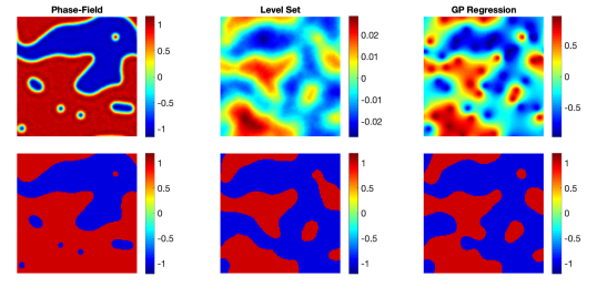
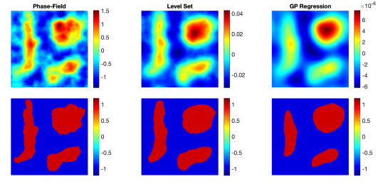
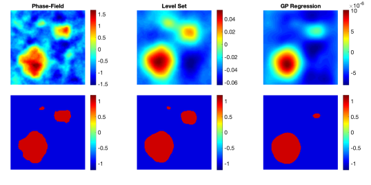
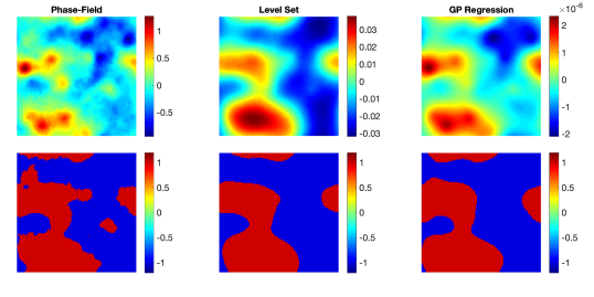
We test the three inversion techniques on three images referred to as Truth A, Truth B and Truth C. These are three fields $u^{\dagger}$ lying in the set of $BV_{\rm binary}$ images and are illustrated in the obvious way in Fig. 1. Truth A and Truth B are observed on a uniform grid of $15\times 15$ points, Truth C is observed at 50 uniformly distributed points, and all of these observations are corrupted by additive Gaussian noise as in equation Eq. 1.1. Pointwise observation does not fit our theory as we assume $K$ is linear on $L^{1}(D)$; however mollification can be used to address this and leads to results which are not different in any substantive way, as noted in [40].

Figure 1: The three true fields used for inversion; the field on the left will be referred to as Truth A, the field in the middle as Truth B and the field on the right as Truth C. The sets of observation points are shown in each figure.

In order to avoid an inverse crime [44], Truth A and Truth B are generated on a square mesh of $2^{16}$ points, and Truth C is generated on a square mesh of $320^{2}$ points, but the Gaussian random fields are constructed over a mesh of $2^{14}$ points ($N=2^{7}$ in Section 4.2). We perform numerical experiments in both the small noise and order one noise regimes.

4.1.1 Small Observational Noise Set-Up

We set $c=3/2$ and $\varepsilon=0.01.$ The implied standard deviation of the observational noise is thus $0.001.$ We make the choices of parameters in the prior covariance operator $C(=C_{\varepsilon,\tilde{\delta},\tilde{a}})$, $a_{1}=0$, $a_{2}=1$, $a_{3}=0$, $b=4$ and $r=1$ for both the Bayesian level set approach and the phase-field approach. For the Bayesian level set approach we set $\delta=1$, $q=0$, $\tau=50$ and $\alpha=3$ whereas for the phase-field approach $\delta=0.01$, $q=0.1$, $\tau=1$ and $\alpha=2$. Thus we ensure that the relations Eq. 3.3 hold so that the phase-field MAP estimator for $\nu^{y}$ approximates the minimizer of $I_{0}^{\delta}$ as given in Theorem 3.4 and we expect the posterior mass to concentrate fairly close to this MAP estimator. Note that in general we need not insist on the parameters being related via Eq. 3.3 for the level set formulation; this is because, unlike the phase-field formulation, there is no MAP estimator whose properties we are seeking to control via parameter choices. For these small noise experiments the GP regression used the same parameters as for the Bayesian level set method.

4.1.2 Order One Observational Noise Set-Up

We set $c=0.$ Note that now $\varepsilon$ does not enter the observational noise; it is simply a parameter that enters the prior and so the phase-field formulation is truly Bayesian. With this choice of $c$ we require, for the phase-field formulation, $a_{1}=-3/2,a_{2}=-1/2,a_{3}=-1,b=1$. We also set $\delta=100$, $q=0.1,\tau=1$, $\alpha=2$ and $r=1$. For the level set formulation we retain the same choice of parameters as for the small noise case above. For the GP regression we use the same parameters as for the phase-field approach for these order one noise experiments.

4.2 Sampling From The Gaussian Prior Space

We describe how to sample numerically from Gaussian priors $\zeta_{0}=\mathcal{N}(0,\mathsf{C})$ that are key to the techniques outlined in the preceding two subsections. Here $\mathsf{C}$ is either $C^{\frac{\alpha}{2}}$ or $C$. We consider the case that $D$ is the unit square $(0,1)^{2}$. Let $\{\lambda_{k}\}$ denote the eigenvalues of $\mathsf{C}$ in increasing order with corresponding $L^{2}(D)$-normalized eigenfunctions (which are Fourier modes) $\{\varphi_{k}\}$. Then samples $z$ from $\zeta_{0}$ may be expressed through the Karhunen-Loève expansion as

(4.1) $$z(x)=\sum_{k=1}^{\infty}\lambda_{k}^{\frac{1}{2}}\xi_{k}\varphi_{k}(x),\quad\xi_{k}\sim\mathcal{N}(0,1)\text{ i.i.d.}$$

We implement an approximation to this by jointly approximating the field via spectral truncation and evaluation on a discrete grid of points. Such an approximation may be efficiently implemented using the Fast Fourier Transform. We work on a uniformly spaced grid $\{x_{i}\}$ of $N^{d}$ points in $D$. An approximate sample on this grid is then given by

$$z^{N}(x_{i})=\sum_{k=1}^{N^{d}}\lambda_{k}^{\frac{1}{2}}\xi_{k}\varphi_{k}(x_{i}),\quad\xi_{k}\sim\mathcal{N}(0,1)\text{ i.i.d.}$$

All of our numerical results are performed on the two dimensional grid which arises from this approach to generating Gaussian random fields in dimension $d=2.$ In practice we choose $N=2^{7}$, and so the discrete grid for our inversion is $2^{14}$ points.

4.3 MCMC Simulation

Markov Chain Monte Carlo (MCMC) simulations may be used to sample measures $\nu^{y}$.

In all MCMC runs we generate $10^{6}$ samples and, when computing means, discard the first $5\times 10^{5}$ samples as burn-in .

We employ the preconditioned Crank-Nicolson (pCN) algorithm [2, 20] which may be used to sample any measure $\sigma$ of the form

$$\frac{\mathrm{d}\sigma}{\mathrm{d}\sigma_{0}}(z)=\frac{1}{Z}\exp\left(-A(z)\right),\quad\sigma_{0}=\mathcal{N}(0,C),$$

without computing derivatives of $A(\cdot).$ Both of our posterior measures can be written in this form. For the Bayesian level set approach we have

$$\frac{\mathrm{d}\nu^{y}}{\mathrm{d}\mu_{0,\alpha}}=\frac{1}{Z}\exp\left(-\frac{1}{2\varepsilon^{2c}}\Bigl{|}\Sigma^{-\frac{1}{2}}\bigl{(}y-KS(v)\bigr{)}\Bigr{|}^{2}\right),$$

whereas for the phase-field approach we have

$$\frac{\mathrm{d}\nu^{y}}{\mathrm{d}\mu_{0}}=\frac{1}{Z}\exp\left(-\frac{r}{\varepsilon^{b}}\int_{D}\frac{1}{4}\bigl{(}1-u(x)^{2}\bigr{)}^{2}\,\mathrm{d}x-\frac{1}{2\varepsilon^{2c}}\Bigl{|}\Sigma^{-\frac{1}{2}}\bigl{(}y-Ku\bigr{)}\Bigr{|}^{2}\right),$$

where $\mu_{0},\mu_{0,\alpha}$ are Gaussian measures, and with the appropriate normalization constants $Z$. The pCN method has the advantage that, unlike the standard Random Walk Metropolis MCMC algorithm, its rate of convergence to equilibrium can be bounded below independently of the number of terms used in the truncated Karhunen-Loève expansion described in Section 4.2 [33].

In the notation of [20] for the pCN algorithm, $\beta\in(0,1]$ denotes the proposal variance parameter. Note that larger $\beta$ tends to lead to smaller acceptance probability, but to greater exploration of state space when steps are accepted; the optimal $\beta$ is a trade-off between these two competing effects. Depending on the noise model and number of observations, we take the proposal standard deviation parameter $\beta$ between $0.02$ and $0.1$ for level set simulations and $\beta$ between $0.002$ and $0.02$ for phase-field simulations. These choices are made in order to balance acceptance rate and size of proposed move with a view to optimizing the convergence rate of the Markov chain.

We simply assume that the resulting Markov chains $\{\eta^{(m)}\}$ are ergodic and make the approximation for an associated measure $\nu^{y}$ that

$${\mathbb{E}}^{\nu^{y}}g(\eta)\approx\frac{1}{M}\sum_{m=1}^{M}g(\eta^{(m)})+e_{M}$$

where the error $e_{M}$ is Gaussian with variance $c_{g}/M$, and $c_{g}$ is the integrated auto-correlation of $g(\eta^{(m)}).$ We do not impose specific stopping criteria on the Markov chains, rather we will examine the approximation qualities derived from the chains, as a function of $M$, and study the convergence to equilibrium of quantities of interest; in particular in Section 4.3.1 we compare the acceptance probability of the chain, as a function of $M$, for the level set and phase-field approaches. The samples up to step $M$ can then be used to produce point estimates for the fields, by calculating, for example, their mean or the sign of their mean. We compare the cost of sampling versus the quality of reconstruction with these point estimates, for differing formulations.

Remark 4.1.

The theory in [33] demonstrates ergodicity for problems similar to those arising in the phase-field formulation. Developing an analogous theory for the level set formulation is an open and interesting research direction; however our numerics do suggest that ergodicity holds in this case too.

Remark 4.2.

Preliminary numerical results for the one dimensional analogue of the problem studied here may be found in [61]. They are consistent with what we report here in dimension two.

4.3.1 Computational Cost

For MCMC sampling, which we use for both the phase-field and level set approaches, every set of the Markov chain requires an evaluation of $A(u).$ Due to the presence of an extra integral term, this evaluation will typically be more expensive for the phase-field model than the level set model; for the simulations performed here, evaluation of $A(u)$ is approximately twice as expensive for the phase-field model than for the level set model. For the GP regression simulations no sampling is required and so the computational cost is significantly cheaper; the means were calculated from the expression in Section 2.3, with the cost arising from the matrix multiplications and inversion involved.

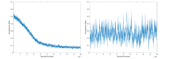
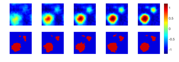
For the phase-field and level set approaches, the most significant discrepancy in computational cost arises from the statistical properties of the Markov chain used to sample the posterior approximately. In Fig. 2 we show the evolution of the local acceptance rates of proposed states for Truth A with small observational noise, as a function of $M$. The evolutions are similar for the other datasets and so are not presented for brevity.The parameter $\beta$, the proposal variance, is chosen so that the acceptance probability is neither close to one nor zero; recall that this results in an order of magnitude smaller value of $\beta$ for the phase-field method in comparison with level set, meaning that the former method makes a much slower exploration of the posterior distribution. Fig. 2 suggests that the phase-field chains have not reached equilibrium until after at least $5\times 10^{5}$ samples, whereas the level set chains converge much earlier. This is illustrated in Fig. 3, which shows a selection of samples for $M=\mathcal{O}(10^{4})$ for Truth B with small observational noise. With $M=10^{4}$ samples, the three inclusions have already been identified by the level set chain, however after $M=3\times 10^{4}$ samples the phase-field chain has only started to identify a second inclusion. Thus, even though for both models we produced the same number of samples, it would have sufficed to terminate the level set chains much earlier, significantly reducing the computational cost.

The fact that the acceptance rates for the phase-field chains are lower than those for the level set chains, despite the proposal standard deviation parameter $\beta$ being one tenth of the size can be understood as follows. Note that the measure $\nu^{y}$ can informally be thought of as having Lebesgue density proportional to $\exp(-J^{\varepsilon}(u))=\exp(-\varepsilon^{-2a_{1}-3}I^{\varepsilon}(u))$. Thus for small $\varepsilon$ the probability mass is concentrated in a small neighborhood of critical points of $I^{\varepsilon}\approx I^{0}_{\delta}$. The MCMC simulations for $\nu^{y}$ could hence be viewed as a form of derivative-free optimization for the functional $J^{\varepsilon}$.

Figure 2: The evolution of the acceptance rate of proposals for the phase-field (left) and level set (right) MCMC chains, for Truth A with small observational noise. Acceptance rates are calculated over a moving window of $1000$ samples.

Figure 3: Examples of samples near the start of chains for Truth B with small observational noise. Sample numbers 10000, 20000, 30000, 40000 and 50000 are shown from left-to-right for the phase-field chain (top) and the level set chain (bottom).

4.4 Reconstruction Of The Means

4.4.1 Small Observational Noise

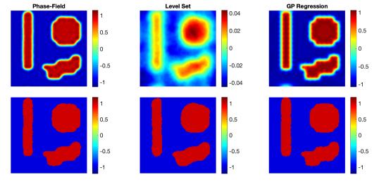
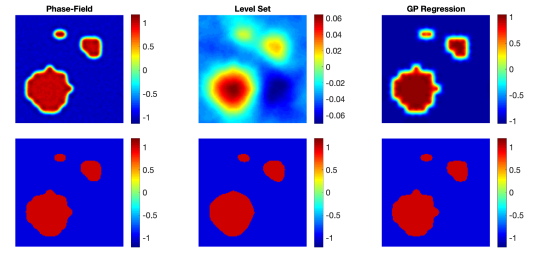
In Fig. 4 we present sample means associated with small-noise observations for the phase-field, level set and GP regression models, both with and without thresholding by $S$. Note that the phase-field and GP regression models attempt to fit the un-thresholded field to the data points, whereas the level set method attempts to fit the thresholded field; the un-thresholded field for the level set method is hence on a different scale to the other two models.

For Truth A and Truth B, the general quality of the reconstruction is similar for all three models after thresholding, though the level set method does not overfit to the datapoints as significantly as the other two methods; this overfitting for the phase-field and GP regression is manifest in a boundary for the largest inclusion in Truth B which has variations on the scale of the observational noise. Another noticeable effect in the quality of the phase-field and GP regression, manifest in Truth A, is that the edges of the circular inclusion are rendered approximately piecewise linear; this might be ameliorated by using a small mesh increment to $\varepsilon$ ratio. The level set method has no small length scale to resolve, and hence does not suffer from this effect.

For all three models reconstruction of Truth C is fairly inaccurate as the sparse observation network does not resolve the length scale on which the true field varies. The level set and GP regression models perform similarly, whereas the phase-field model places much more mass into the positive class; it is likely that this reflects a lack of convergence of the Markov chain for the phase-field model.

Figure 4: Sample means for Truth A (top block), Truth B (middle block) and Truth C (bottom block) with small observational noise. To top row of each block shows Monte Carlo approximations to $\mathbb{E}^{\nu^{y}}(v)$, the underlying continuous fields, and the bottom row in each block shows Monte Carlo approximations to $S\big{(}\mathbb{E}^{\nu^{y}}(v)\big{)}$, the thresholded fields.

Figure 5: Sample means for Truth A (top block), Truth B (middle block) and Truth C (bottom block) with order one observational noise. To top row of each block shows Monte Carlo approximations to $\mathbb{E}^{\nu^{y}}(v)$, the underlying continuous fields, and the bottom row in each block shows Monte Carlo approximations to $S\big{(}\mathbb{E}^{\nu^{y}}(v)\big{)}$, the thresholded fields.

4.4.2 Order One Noise Reconstructions

In Fig. 5 the sample means associated with order one observational noise are shown. As would be expected, reconstruction quality is generally poorer than for the small-noise observations, though overfitting to the observational noise is no longer an issue for the phase-field and GP approaches. The three models perform similarly, though there seems to be an increased amount of penalization on the length of the interface from left-to-right. Without thresholding, the GP regression means provide poor estimates of the truth in terms of scale, due to the far weaker influence of the likelihood and lack of prior information enforcing values close to $\pm 1$.

4.5 Perimeter Learning

Here we study perimeter learning for the Bayesian level set method. The length of the zero level set of $\eta^{N}$ may then be approximated by using the discrete variation of $w^{N}:=S(\eta^{N})$,

$$\ell(N)=\frac{1}{2N^{2}}\sum_{i,j=1}^{N}{|\mathsf{D}^{N}w^{N}(x_{i},y_{j})|}\approx\frac{1}{2}\int_{D}|\nabla w^{N}(x,y)|\,$$

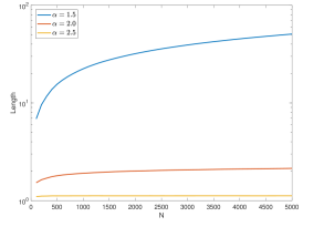
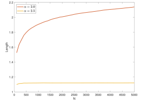
where the operator $\mathsf{D}^{N}$ approximates the gradient on the grid $\{x_{i},y_{j}\}$ via central differences. Using this we investigate numerically the length of the level sets of these samples. We have shown in Lemma 2.1 that choosing $\alpha>1+d/2$ is sufficient to ensure almost sure finite length of level sets. Numerical experiments indicate that this is a sharp result. In Fig. 6 interface lengths for prior distributions approximated as described above for a single realization of $\{\xi_{k}\}$ in Eq. 4.1 are displayed as a function of $N$ for varying values of $\alpha$. We use $d=2$ and observe that for $\alpha<2$ the length of the interface diverges algebraically with $N$ (left hand panel), for $\alpha=2$ it diverges logarithmically (right hand panel shows this best), and for $\alpha>2$ it converges to a constant (both left and right hand panels show this). The results, then, suggest that level sets have finite length almost surely if and only if $\alpha>1+d/2.$

Figure 6: The dependence of the length of the zero level set of a Gaussian sample, as a function of numerical approximation level $N$ and of prior regularity parameter $\alpha$. (Left) logarithmic axis, (right) linear axis.

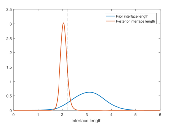
In order to compare the perimeter distribution between the prior and posterior, the choice $\alpha>1+d/2$ ensures that the length of the zero level set is well-defined so in two dimensions we take $\alpha=3$. The results for recovery of Truth B are shown in Fig. 7. Whilst the perimeter still retains some variation under the posterior, the variation is much lower and, in contrast to the prior, it is concentrated around the true value of the perimeter. We see that though the Bayesian level set approach does not explicitly penalize the perimeter, it has the ability to estimate the perimeter, and quantify uncertainty in the estimation.

Figure 7: The distribution of the perimeter under the prior and posterior distribution. The vertical dashed line indicates the perimeter of the true field.

5 Eikonal Equation

In this section we build on what we have learned so far for the linear inverse problem defined by (1.1) and use it to study a nonlinear inverse problem from the eikonal equation. Gaussian process regression is fast to implement, and appears to give qualitatively comparable accuracy to the Bayesian level set method; but it does not generalize to nonlinear problems and so we do not consider it further. The experiments in the previous section, set-up in Section 4.1, suggest that the Bayesian level set approach to binary recovery has two advantages over the Bayesian phase-field formulation, for the linear inverse problem considered: the level set method is faster and draws from the posterior contain information about the true perimeter. Thus we focus attention purely on the Bayesian level set method. Within this context we also demonstrate the benefits of hierarchical Bayesian inversion.

5.1 The Forward Equation

Let $x_{0}\in D$ be a wave emitting source, and define the first arrival time of the wave at $x\in D$ as $T(x)$. The wave passes through a medium which adjusts the wave speed according to a scalar function $u\colon D\to\mathbb{R}_{+}$ known as the slowness. It is shown in [49, 62] that $T(x)$ may be viewed as solution of a stationary Hamilton-Jacobi equation, namely the following eikonal equation:

(5.1) $$|\nabla T(x)|=u(x), \forall x\in D\setminus\{x_{0}\},$$

(5.2) $$T(x_{0})=0,$$

(5.3) $$\nabla T(y)\cdot n(y)\geq 0, \forall y\in\partial D,$$

where $n$ is the outward pointing unit normal. The Soner boundary condition (5.3) ensures ray paths terminate at $\partial D$ [62]. The recovery of the slowness function $u$ from observations of arrival times is known as first arrival traveltime tomography. Extensive discussion of the well-posedness of the forward problem can be found in [24, 25, 30]. For our application, we consider a binary slowness function $u\colon D\to\{u_{\min},u_{\max}\}$ where $0<u_{\min}\leq u_{\max}$.

We define the solution map $\mathsf{G}$ mapping the slowness $u$ to the travel times $T$ via solution of the eikonal equation with source $x_{0}$. Because we are interested in binary slowness functions we also introduce

(5.4) $$\mathsf{S}(v)=S(v)\cdot(u_{\max}-u_{\min})/2+(u_{\max}+u_{\min})/2;$$

here $S(v)$, is the sign function defined in Section 2.1.

To solve the forward problem we first discretize using an upwind finite difference scheme. We then use a fast marching procedure (see [59]) to solve the discrete eikonal equation. A formulation of the discretization and marching algorithm, along with a proof of numerical convergence is found in [25].

5.2 The Bayesian Inverse Problem

Let $\eta\sim\mathcal{N}(0,\Sigma)$ be a normal random variable in $\mathbb{R}^{J}$. Fix $x_{0}\in\bar{D}$. Defining the observation map $K$ taking traveltimes to $\mathbb{R}^{J}$ we define the inverse problem of finding $v$, given observed data $y$ satisfying

(5.5) $$y=K\circ\mathsf{G}\circ\mathsf{S}(v)+\varepsilon^{c}\eta=K\circ\mathsf{G}(u)+\varepsilon^{c}\eta.$$

We will assume that $K$ is defined so that the data $y$ is a set of observed first hitting times at fixed known receiver locations $\{z_{j}\}_{j=1}^{J}\in\bar{D}$. The random variable $y|v\sim\mathcal{N}(K\circ\mathsf{G}\circ\mathsf{S}(v),\varepsilon^{2c}\Sigma)$, leading to negative log likelihood defined, up to an additive constant, by

$$\Phi(v;y)=\frac{1}{2\varepsilon^{2c}}\left|\Sigma^{-\frac{1}{2}}\big{(}y-K\circ\mathsf{G}\circ\mathsf{S}(v)\big{)}\right|^{2}.$$

We will treat problems of multiple sources $\{x_{0}^{m}\}_{m=0}^{M}$ as multiple experiments, with solution maps $\mathsf{G}^{m}$ each producing data $y^{m}\in\mathbb{R}^{J}$. The natural extension is to consider the following negative log likelihood,

(5.6) $$\Phi(v;y)=\frac{1}{2\varepsilon^{2c}}\sum_{m=1}^{M}\left|\Sigma^{-\frac{1}{2}}\big{(}y^{m}-K\circ\mathsf{G}^{m}\circ\mathsf{S}(v)\big{)}\right|^{2},$$

for the $m$ observations $y=(y^{1},\dots,y^{m}).$ We assume that we are given prior measure $\zeta_{0}=\mathcal{N}\bigl{(}0,\mathsf{C}\bigr{)}$ and let $\zeta^{y}(\mathrm{d}v)$ denote the probability distribution of the conditioned random variable $v|y$. Then using Bayes’ theorem (see Proposition 2.3), we deduce that $\zeta^{y}$ is a probability measure supported on continuous functions, determined by

$$\frac{\,\mathrm{d}\zeta^{y}}{\,\mathrm{d}\zeta_{0}}=\frac{1}{Z}\exp\Big{(}-\frac{1}{2\varepsilon^{2c}}\sum_{m=1}^{M}\Big{|}\Sigma^{-\frac{1}{2}}\big{(}y^{m}-K\circ\mathsf{G}^{m}\circ\mathsf{S}(v)\big{)}\Big{|}^{2}\Big{)},$$

with normalization constant $Z$. This problem has been formulated for piecewise constant slowness function with Ginzburg-Landau type regularization in the deterministic setting [30], where simulations and proofs of convergence of numerical schemes can be found. We choose here to use a level set formulation for the reasons discussed at the start of the section.

5.2.1 Hierarchical Inference For Inverse Lengthscale

In hierarchicalBayesian inference we employ a Gaussian prior measure $\zeta_{0}=\mathcal{N}(0,\mathsf{C}(\tau))$ in which the covariance $\mathsf{C}$ depends on parameter $\tau>0$ which we interpret as an additional unknown to be learned during the inversion process. In particular we will work with settings in which $\tau$ has interpretation as an inverse length-scale. To this end, define the hierarchical prior $\zeta_{0}$ by decomposing as follows:

$$\zeta_{0}(\mathrm{d}v,\mathrm{d}\tau)=\zeta_{0}(\mathrm{d}v|\tau)\pi_{0}(\tau)\,\mathrm{d}\tau.$$

We call $\pi_{0}(\tau)$ the hyperprior. Generalizing the derivation of the posterior in the preceding subsection, we now find that the distribution of $v,\tau|y$ is determined by probability measure $\zeta^{y}(\mathrm{d}v,\mathrm{d}\tau)$ defined by

(5.7) $$\zeta^{y}(\mathrm{d}v,\mathrm{d}\tau)=\frac{1}{Z}\exp(-\Phi(v;y))\zeta_{0}(\mathrm{d}v|\tau)\pi_{0}(\tau)\,\mathrm{d}\tau,$$

for normalization constant $Z$. For reasons discussed in [53, 68] it can be advantageous to reparameterise the hierarchical inverse problem in terms of $(\xi,\tau)$, rather than $(v,\tau)$, where $\xi$ is a Gaussian white noise distributed as $\mathcal{N}(0,I),$ so that $v=\sqrt{\mathsf{C}(\tau)}\xi;$ the underlying latent Gaussian white noise $\xi$ may be identified with the collection of i.i.d. unit Gaussians $\{\xi_{k}\}$ used to construct prior samples in Section 4.2. Abusing notation we may write the posterior distribution $\zeta^{y}$, now for the variable $(\xi,\tau)$, as

(5.8) $$\zeta^{y}(\mathrm{d}\xi,\mathrm{d}\tau)=\frac{1}{Z}\exp(-\Phi(\sqrt{\mathsf{C}(\tau)}\xi;y))\zeta_{0}(\mathrm{d}\xi)\pi_{0}(\tau)\,\mathrm{d}\tau.$$

Working with variables $(v,\tau)$ as in (5.7) is refered to as the centred problem formulation; using variables $(\xi,\tau)$ as in (5.8) is refered to as the non-centred problem formulation.

Numerical evidence described in [31, 15] demonstrates that for level-set based inverse problems use of the non-centered formulation in (5.8) confers considerable advantages in terms of speed of convergence of MCMC. We thus employ the non-centered formulation. To sample from this distribution we use [15, Algorithm 6.1], known as the non-centred pCN-within-Gibbs. This algorithm updates $\xi$ and $\tau$ in separate substeps of a pCN sampling method, and we perform this in a random order each iteration.

5.2.2 Hierarchical Inference For Contrast

We also consider a model hyperparameter that originates in the application (whereas $\tau$ appears when regularizing through the prior). We investigate the contrast between the binary materials, and rewriting the relationship between $u$ and $v$, we obtain

$$\mathsf{S}(v)=\frac{\kappa}{2}(S(v)+1)+u_{\min},$$

where $\kappa=(u_{\max}-u_{\min})>0$ is the contrast. Knowing the parameter $u_{\min}$, we consider the parameter $\kappa$ as a positive random variable to be learnt from the data. This increases flexibility of techniques in application as we can apply our methods to scenarios where slowness contrast is uncertain. We may include this in a non-centred pCN-within-Gibbs algorithm as above, by exploiting the form

$$\mathsf{S}(v)=\frac{\kappa}{2}(S(\sqrt{\mathsf{C}(\tau)}\xi)+1)+u_{\min},$$

substituting this into the likelihood (5.6). We update each of $\xi,\tau,\kappa$ separately and in random order in each iteration.

5.2.3 Numerical Results: Lengthscale Hyperparameter Only

Figure 8: The sign of fields $v$, where $\mathsf{S}(v)$ (for appropriate $u_{\min}$, $u_{\max}$) will be used as a truth for inversion; the field on the left will be referred to as Truth D and the field on the right as Truth E. The sets of observation ($\times$) and source ($+$) points are shown in each figure.

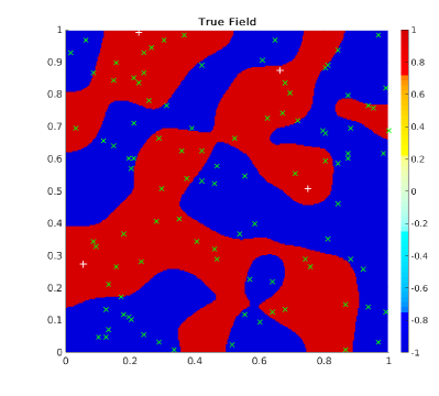
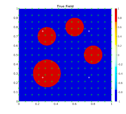
For this first test we wish to demonstrate recovery of hyperparameters with the nonlinear eikonal forward model as described in Section 5.2.1. Our domain is given by $D=[0,1]\times[0,1]$. We choose Truth D as seen in Fig. 8; here the truth has been produced by applying the slowness function $\mathsf{S}(v^{*})$ for an instance $v^{*}\sim\mu_{0}(\tau^{*})$ with hyperparameter $\tau^{*}=\exp(6.5)$. We take $u_{\min}=1.0$, and a known contrast $\kappa=0.2$ (thus $u_{\max}=1.2$).

The discretization uses an equidistributed mesh with grid spacing $h=128^{-1}$. To avoid an inverse crime we produce the data on a numerical mesh with spacing $h/2$. We take 4 sources $\{x^{m}_{0}\}_{m=1}^{4}$ and 100 receivers uniformly distributed in the (coarser) discrete domain.

We work with the parameters same as taken in Section 4.1.1 with the exception of setting $c=1$ and, of course, viewing $\tau$ as an unknown. For consistency across different source–receiver combinations we additionally scale the noise by the range of the traveltime observations, so the effective observational noise is $10^{-2}$. We take $\alpha=3$ to ensure finite perimeter.

For the hyperparameter $\tau$, we choose a lognormal prior to ensure positivity, we take prior $\pi(\log\tau)=\mathcal{N}(5,2.5)$ and initialize the Markov chain at $\log(3)$. We use the non-centred pCN-within-Gibbs algorithm [15, Algorithm 6.1] described in Section 5.2.1 with a random walk Metropolis proposal for the hyperparameter step. The step sizes were chosen to achieve $20\%-25\%$ acceptance rates for $\xi$ and $\tau$.

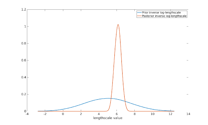
The result of the recovery of truth D after $2\times 10^{5}$ iterations run is displayed in Fig. 9. The recovery of the field is fairly faithful; we note that information can only be learnt between source and receiver pairs, see Truth D in Fig. 8 for their random distribution. We additionally provide the distribution of the perimeter in Fig. 10 with true perimeter marked, and one can see that this falls well within the posterior distribution with high probability mass given to a small neighborhood of the truth. In Fig. 11 we see the results of learning the hyperparameter distribution. We see the marked truth and the prior and posterior distribution, and again we see the posterior peaks near the true value and gives large mass to a small neighborhood of the truth. We note that the parameter $\log\tau$ is sampling close to its posterior within $10^{4}$ iterations in this example.

Figure 9: Sample means for truth D. The left shows the Monte Carlo approximation of $\mathbb{E}^{\mu^{y}}(v)$, the underlying continuous field. The right shows the Monte Carlo approximation of $\mathsf{S}(\mathbb{E}^{\mu^{y}}(v))$, the thresholded and scaled field.

Figure 10: The distribution of the perimeter under the prior and posterior distribution for truth D. The vertical dashed line indicates the perimeter of the true field.

Figure 11: The distribution of the logarithm of the hyperparameter $\tau$ under the prior and posterior distribution for truth D. The vertical dashed line indicates the hyperparameter value $\log\tau=6.5$ of the true field.

5.3 Numerical Results: Lengthscale And Contrast Hyperparameters

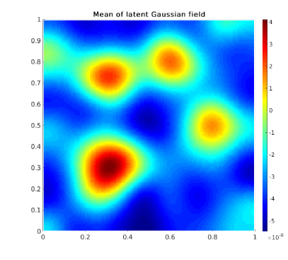
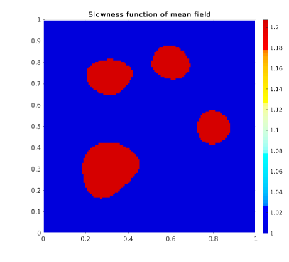
For this test we demonstrate recovery of the contrast in the medium. We assume that we are in the situation of performing the inverse eikonal problem where we do not have exact information on the contrast between the binary phases. We choose Truth E as seen in Fig. 8, comprising four circles; three of diameter $0.1$ and one of diameter $0.15$. In the figure we see the choice of four sources, and take $15^{2}$ equally spaced receivers over the domain. We take $u_{\min}=1.0$, and again we work with the parameters as detailed in Section 4.1.1 with the exception of setting $c=1$, and viewing $\tau$ as unknown and, as in the previous subsection, we set $\alpha=3$. We assume the contrast is lognormal with prior $\pi(\log\kappa)=\mathcal{N}(\log(0.2),0.3)$, as we require a positive prior, we also treat $\tau$ as a random unknown quantity, and take a lognormal $\pi(\log\tau)=\mathcal{N}(5,2.5)$. We initialize the MCMC method to sample these variables at $\log\tau=8$ and $\log\kappa=\log(0.1)$.

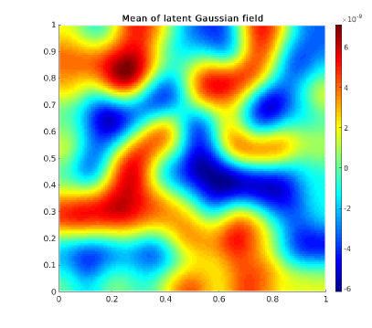
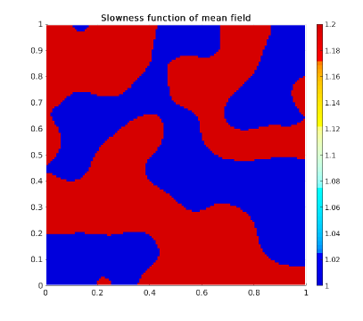
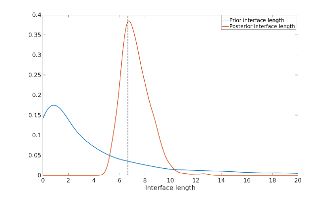
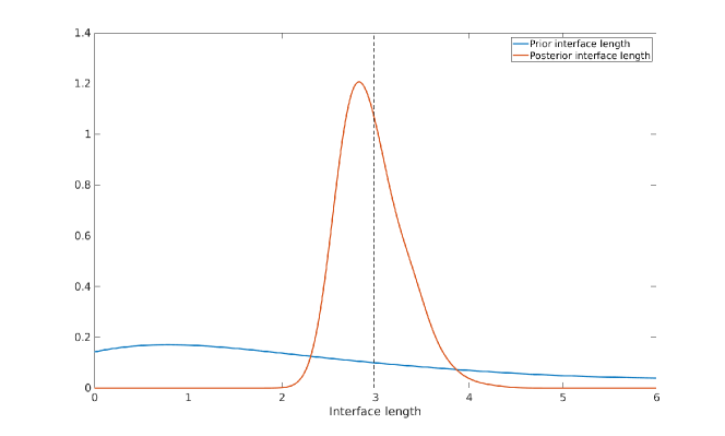
Our recovery of Truth E after $2\times 10^{5}$ iterations is recorded in Fig. 12. We see an excellent recovery of the simple geometry, in particular the colorscale shows the approximation of the mean recovered contrast to the true contrast, where $u_{\min}=1,\ u_{\max}=1.2$. This recovery is demonstrated in Fig. 13 where we see the prior and posterior densities for the interfacial length. The posterior places most weight in a small neighbourhood of the truth, and peaks nearby.

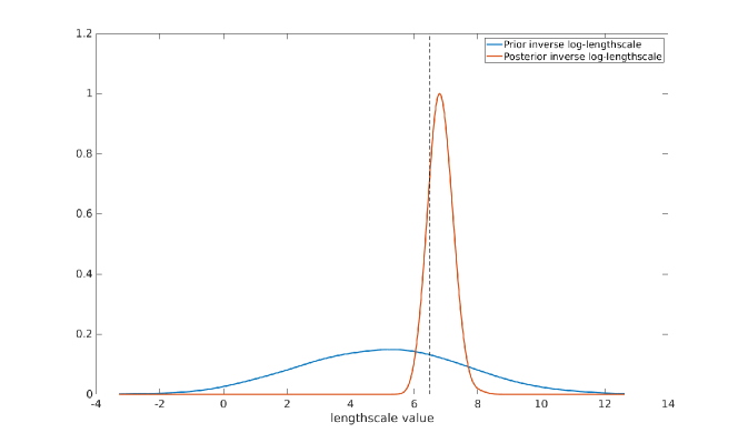
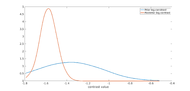
The hyperparameter recovery is displayed in Fig. 14 and Fig. 15. We see the profiles for prior and posterior for $\log\tau$ in Fig. 14, demonstrating that the posterior concentrates within a sensible range; note that there is no true $\tau$ for this example. In Fig. 15 we see the contrast recovery, and observe that the posterior places large weight close to the true value. It again takes less than $10^{4}$ iterations for both hyperparameters to draw approximately from their posterior distributions.

Figure 12: Sample means for truth E. The left shows the Monte Carlo approximation of $\mathbb{E}^{\mu^{y}}(v)$, the underlying continuous field. The right shows the Monte Carlo approximation of $\mathsf{S}(\mathbb{E}^{\mu^{y}}(v))$, the thresholded and scaled field.

Figure 13: The distribution of the perimeter under the prior and posterior distribution for truth E. The vertical dashed line indicates the perimeter of the true field.

Figure 14: The distribution of the logarithm of $\tau$ under the prior and posterior distribution for truth E.

Figure 15: The distribution of the logarithm of $\kappa$ under the prior and posterior distribution for truth E. The vertical dashed line indicates true value $\log\kappa=\log(0.2)$.

6 Conclusions

The paper investigates the reconciliation of perimeter and Bayesian regularization for the reconstruction of functions with interfaces, from direct or indirect noisy measurements. Three approaches are studied: Formulation 1 is based on Bayesian level method; Formulation 2 is based on Bayesian phase-field regularization; and Formulation 3 is based on Gaussian process regression and classification.

By studying a class of linear inverse problems we show that Formulation 2 exhibits perimeter regularization in the context of its MAP estimator, but not at the level of samples from the posterior distribution. Formulation 1 exhibits perimeter regularization at the level of individual samples from the posterior; there is no MAP estimator in this context. Both Formulations 1 and 2 require careful choices of constants in construction of the prior, but Formulation 2 is far more constrained in this regard. Furthermore, as a consequence of these constraints, Formulation 2 exhibits a measure concentration phenomenon meaning that MCMC based algorithms using Formulation 1 are considerably faster than those based on Formulation 2. Formulation 3 is competitive with Formulation 1 in terms of both sample properties and speed, but does not generalize beyond linear problems. We study Formulation 1 for a nonlinear inverse problem, demonstrating that it is effective in this context and, in addition, showing how hierarchical methods may be used to learn model hyper-parameters appearing in the prior.

The ideas in this paper can be combined in different ways: the methodology may be extended beyond binary-valued functions to a variety of piecewise continuous problems; or other limiting functionals could be contemplated, such as Mumford-Shah [36]; and other smoothed thresholding functions could be contemplated within the level set method, such as the double-obstacle approximation to the signum function [3, 4]. The success of the Bayesian level set method suggests that further analysis of it, as well as its deployment in new application domains, would be very valuable.

Appendix A Proofs Of Main Results

Proof of Proposition 3.2. Throughout this proof $C$ is a universal constant whose value may change between occurrences. To apply Theorem 4.12 from [21], we need to show that the function $\Phi(\cdot,y)$ is bounded from below, is locally bounded from above and is locally Lipschitz. We note that $\Phi(\cdot,y)$ is always non-negative so is bounded from below. If $\|u\|_{X}=\max_{x\in\bar{D}}|u(x)|\leq\rho$ then we may bound $|\Phi(u,y)|$ by a constant depending on $\rho$ i.e. $\Phi(\cdot,y)$ is locally bounded. For the local Lischiptz continuity, we have

$$\Phi(u,y)-\Phi(v,y)=\frac{r}{4\varepsilon^{b}}\int_{D}(2-u(x)^{2}-v(x)^{2})(u(x)+v(x))(u(x)-v(x))\,\mathrm{d}x+$$

$$\frac{1}{2\varepsilon^{2c}}\langle\Sigma^{-\frac{1}{2}}(2y-Ku-Kv),\Sigma^{-\frac{1}{2}}K(v-u)\rangle$$

Assume that $\|u\|_{X}\leq\rho$ and $\|v\|_{X}\leq\rho$. Then, since $K$ is a bounded linear operator on $L^{1}(D),$

$$|\Phi(u,y)-\Phi(v,y)|\leq C\int_{D}|u(x)-v(x)|dx+C|K(v-u)|$$

$$\leq C\|u-v\|_{L^{1}(D)}\leq C|D|^{1/2}\|u-v\|_{L^{2}(D)}\leq C\|u-v\|_{X}.$$

The desired result follows. $\Box$

Proof of Theorem 3.4. We adapt the proof of Hilhorst et al. to allow for periodic boundary conditions and the additional $L^{2}$ norm appearing in the functional to be infimized. From Hilhorst et al., we have that if $u^{\varepsilon}\to u$ in $L^{1}(D)$ then

$$\liminf_{\varepsilon\to 0}I^{\varepsilon}(u^{\varepsilon}) \geq \liminf_{\varepsilon\to 0}\int_{D}\left(\frac{1}{2}{\delta\varepsilon^{3}}|\triangle u^{\varepsilon}|^{2}+\frac{1}{2}\delta q\varepsilon|\nabla u^{\varepsilon}|^{2}+\frac{r}{4\varepsilon}\bigl{(}1-u^{\varepsilon}(x)^{2}\bigr{)}^{2}\right)\mathrm{d}x$$

$$+\frac{1}{2}|\Sigma^{-\frac{1}{2}}(y-Ku^{\varepsilon})|^{2}$$

$$\geq I_{0}^{\delta}(u).$$

Now we show that for each $u\in L^{1}(D)$, there is a sequence $\{u^{\varepsilon}\}\subset H^{2}_{\#}(D)$ which converges strongly to $u$ in $L^{1}(D)$ such that $\limsup_{\varepsilon\to 0}I^{\varepsilon}(u^{\varepsilon})\leq I_{0}^{\delta}(u)$. We first review the main points in the proof of Hilhorst et al. for functions $u\in H^{2}(D)$. Considering the case $I^{\delta}(u)<\infty$, without loss of generality, we assume that

$$u=\mathds{1}_{Q}-\mathds{1}_{\mathbb{R}^{d}\setminus Q}$$

where $Q$ is a bounded domain, with $\partial Q\in C^{\infty}$ and $Q\subset\subset D$. The sign distance function is defined as

$$d(x)=\left\{\begin{array}[]{rl}+\inf_{y\in\partial Q}|x-y|\ \mbox{if}\ x\in Q\\ -\inf_{y\in\partial Q}|x-y|\ \mbox{if}\ x\notin Q\end{array}\right.$$

Let $N_{h}$ be an $h$ neighbourhood of $\partial Q$ (we choose $h$ so that $h$ is less than the distance between $\partial Q$ and $\partial D$.) We choose a function $\eta\in C^{2}(\bar{D})$ such that $\eta(x)=d(x)$ for $x\in N_{h}$, $\eta(x)\geq h$ when $x\in Q\setminus N_{h}$ and $\eta(x)\leq-h$ when $x\in D\setminus(Q\bigcup N_{h})$. Let $U$ be an odd minimizer of the functional $e^{\delta}(U)$ with $\lim_{t\to\infty}U(t)=1$ and $\lim_{t\to-\infty}U(t)=-1$. We let

$$u^{\varepsilon}=U\left(\frac{\eta(x)}{\varepsilon}\right).$$

We note that $u^{\varepsilon}(x)$ is uniformly bounded pointwise and $u^{\varepsilon}(x)\to u(x)$ for all $x\in D$. From the Lebesgue dominated convergence theorem, $u^{\varepsilon}\to u$ in $L^{1}(D)$ and in $L^{2}(D)$. Thus

$$\lim_{\varepsilon\to 0}|\Sigma^{-\frac{1}{2}}(y-Ku^{\varepsilon})|^{2}=|\Sigma^{-\frac{1}{2}}(y-Ku)|^{2}.$$

and, since $a>0$,

$$\lim_{\varepsilon\to 0}\int_{D}\delta\tau^{2}\varepsilon^{a}u^{\varepsilon}(x)^{2}\,\mathrm{d}x=0.$$

To show that $\lim_{\varepsilon\to 0}I^{\varepsilon}(u)=I^{\delta}_{0}(u)$, we follow the approach of Hilhorst et al.. The integral

$$\int_{D}\left(\frac{1}{2}{\delta\varepsilon^{3}}|\triangle u^{\varepsilon}|^{2}+\frac{1}{2}\delta q\varepsilon|\nabla u^{\varepsilon}|^{2}+\frac{r}{4\varepsilon}\bigl{(}1-u^{\varepsilon}(x)^{2}\bigr{)}^{2}\right)\mathrm{d}x$$

is written as

$$\int_{D\setminus N_{h}}\left(\frac{1}{2}{\delta\varepsilon^{3}}|\triangle u^{\varepsilon}|^{2}+\frac{1}{2}\delta q\varepsilon|\nabla u^{\varepsilon}|^{2}+\frac{r}{4\varepsilon}\bigl{(}1-u^{\varepsilon}(x)^{2}\bigr{)}^{2}\right)\mathrm{d}x$$

$$+\int_{N_{h}}\left(\frac{1}{2}{\delta\varepsilon^{3}}|\triangle u^{\varepsilon}|^{2}+\frac{1}{2}\delta q\varepsilon|\nabla u^{\varepsilon}|^{2}+\frac{r}{4\varepsilon}\bigl{(}1-u^{\varepsilon}(x)^{2}\bigr{)}^{2}\right)\mathrm{d}x.$$

Using the exponential decay of $U,U^{\prime}$ and $U^{\prime\prime}$ at $\infty$ and $-\infty$, we deduce that the integral over $D\setminus N_{h}$ goes to $0$ when $\varepsilon\to 0$ (note that $|\eta(x)|/\varepsilon>h/\varepsilon$ which goes to $\infty$ when $\varepsilon\to 0$ for $x\in D\setminus N_{h}$). The integral over $N_{h}$ is shown to converge to $I^{\delta}(u)$ when $\varepsilon\to 0$.

To adapt this proof of Hilhorst et al. to functions with periodic boundary condition on $D$, we only need to choose the function $\eta$ so that $\eta$ is periodic and $\eta(x)\geq h$ when $x\in Q\setminus N_{h}$ and $\eta(x)\leq-h$ when $x\in D\setminus(Q\bigcup N_{h})$. Such a function can be constructed as follows. Let $\psi(x)\in C^{\infty}_{0}(D)$ be such that $\psi(x)=1$ when $x$ is in a neighbourhood of $Q\bigcup N_{h}$, and $0\leq\psi(x)\leq 1$ for all $x\in D$. Let $\eta_{1}(x)$ be a smooth periodic function with $\eta_{1}(x)\leq-h$ for all $x\in D$. Using the function $\eta$ of Hilhorst et al., we define a new function

$$\bar{\eta}(x)=\psi(x)\eta(x)+(1-\psi(x))\eta_{1}(x).$$

The function $\bar{\eta}(x)$ satisfies the requirement. $\Box$

References

- [1] S. Agapiou, M. Burger, M. Dashti, and T. Helin, Sparsity-promoting and edge-preserving maximum a posteriori estimators in non-parametric Bayesian inverse problems, Inverse Problems, 34 (2018), p. 045002.
- [2] A. Beskos, G. O. Roberts, A. M. Stuart, and J. Voss, MCMC methods for diffusion bridges, Stochastics and Dynamics, 8 (2008), pp. 319–350.
- [3] J. Blowey and C. Elliott, Curvature dependent phase boundary motion and parabolic double obstacle problems, in Degenerate Diffusions, Springer, 1993, pp. 19–60.
- [4] J. Blowey and C. Elliott, A phase-field model with a double obstacle potential, Motion by mean curvature and related topics (Trento, 1992), (1994), pp. 1–22.
- [5] C. Brett, C. M. Elliott, and A. S. Dedner, Phase field methods for binary recovery, in Optimization with PDE Constraints, Springer, 2014, pp. 25–63.
- [6] M. Burger and F. Lucka, Maximum a posteriori estimates in linear inverse problems with log-concave priors are proper Bayes estimators, Inverse Problems, 30 (2014), p. 114004.
- [7] D. Calvetti and E. Somersalo, A Gaussian hypermodel to recover blocky objects, Inverse Problems, 23 (2007), p. 733.
- [8] D. Calvetti and E. Somersalo, Hypermodels in the Bayesian imaging framework, Inverse Problems, 24 (2008), p. 034013.
- [9] D. Calvetti, E. Somersalo, and A. Strang, Hierachical bayesian models and sparsity: ? 2-magic, Inverse Problems, 35 (2019), p. 035003.
- [10] M. Cardiff and P. Kitanidis, Bayesian inversion for facies detection: An extensible level set framework, Water Resources Research, 45 (2009).
- [11] M. Carriero, A. Leaci, and F. Tomarelli, A survey on the blake–zisserman functional, Milan Journal of Mathematics, 83 (2015), pp. 397–420.
- [12] J. N. Carter and D. A. White, History matching on the Imperial College fault model using parallel tempering, Computational Geosciences, 17 (2013), pp. 43–65.
- [13] T. F. Chan and X.-C. Tai, Level set and total variation regularization for elliptic inverse problems with discontinuous coefficients, Journal of Computational Physics, 193 (2004), pp. 40–66.
- [14] H. Chang, D. Zhang, and Z. Lu, History matching of facies distribution with the enkf and level set parameterization, J. Comput. Phys., 229 (2010), pp. 8011–8030, https://doi.org/10.1016/j.jcp.2010.07.005, http://dx.doi.org/10.1016/j.jcp.2010.07.005.
- [15] V. Chen, M. M. Dunlop, O. Papaspiliopoulos, and A. M. Stuart, Robust MCMC sampling with non-gaussian and hierarchical priors in high dimensions, arXiv preprint arXiv:1803.03344v2, (2019).
- [16] R. Choksi, Y. van Gennip, and A. Oberman, Anisotropic total variation regularized l^ 1-approximation and denoising/deblurring of 2d bar codes, arXiv preprint arXiv:1007.1035, (2010).
- [17] C. Clason, T. Helin, R. Kretschmann, and P. Piiroinen, Generalized modes in Bayesian inverse problems, SIAM/ASA Journal on Uncertainty Quantification, 7 (2019), pp. 652–684.
- [18] J. Cockayne, C. J. Oates, T. Sullivan, and M. Girolami, Bayesian probabilistic numerical methods, SIAM Review, 61 (2019), pp. 756–789.
- [19] A. Cohen and J.-P. D’Ales, Nonlinear approximation of random functions, SIAM Journal on Applied Mathematics, 57 (1997), pp. 518–540.
- [20] S. L. Cotter, G. O. Roberts, A. M. Stuart, D. White, et al., MCMC methods for functions: modifying old algorithms to make them faster, Statistical Science, 28 (2013), pp. 424–446.
- [21] M. Dashti, K. J. Law, A. M. Stuart, and J. Voss, MAP estimators and their consistency in Bayesian nonparametric inverse problems, Inverse Problems, 29 (2013), p. 095017.
- [22] M. Dashti and A. M. Stuart, The Bayesian approach to inverse problems, arXiv preprint arXiv:1302.6989, (2013).
- [23] K. Deckelnick, G. Dziuk, and C. M. Elliott, Computation of geometric partial differential equations and mean curvature flow, Acta Numerica, 14 (2005), pp. 139–232.
- [24] K. Deckelnick and C. M. Elliott, Uniqueness and error analysis for Hamilton-Jacobi equations with discontinuities, Interfaces and free boundaries, 6 (2004), pp. 329–349.
- [25] K. Deckelnick, C. M. Elliott, and V. Styles, Numerical analysis of an inverse problem for the Eikonal equation, Numerische Mathematik, 119 (2011), p. 245.
- [26] K. Deckelnick, C. M. Elliott, and V. Styles, Double obstacle phase field approach to an inverse problem for a discontinuous diffusion coefficient, Inverse Problems, 32 (2016), p. 045008.
- [27] P. Diaconis, Bayesian numerical analysis, Statistical Decision Theory and Related Topics IV, 1 (1988), pp. 163–175.
- [28] O. Dorn and D. Lesselier, Level set methods for inverse scattering-some recent developments, Inverse Problems, 25 (2009), p. 125001, http://stacks.iop.org/0266-5611/25/i=12/a=125001.
- [29] O. Dorn and R. Villegas, History matching of petroleum reservoirs using a level set technique, Inverse Problems, 24 (2008), p. 035015, http://stacks.iop.org/0266-5611/24/i=3/a=035015.
- [30] O. Dunbar and C. M. Elliott, Binary recovery via phase field regularization for first-arrival traveltime tomography, Inverse Problems, (2019).
- [31] M. M. Dunlop, M. A. Iglesias, and A. M. Stuart, Hierarchical Bayesian level set inversion, Statistics and Computing, 27 (2017), pp. 1555–1584.
- [32] H. W. Engl, M. Hanke, and A. Neubauer, Regularization of inverse problems, vol. 375, Springer Science & Business Media, 1996.
- [33] M. Hairer, A. M. Stuart, and S. J. Vollmer, Spectral gaps for Metropolis-Hastings algorithms in infinite dimensions, The Annals of Applied Probability, 24 (2014), pp. 2455–290, https://doi.org/10.1214/13-AAP982.
- [34] P. C. Hansen, J. G. Nagy, and D. P. O’leary, Deblurring images: matrices, spectra, and filtering, SIAM, 2006.
- [35] T. Helin and M. Burger, Maximum a posteriori probability estimates in infinite-dimensional Bayesian inverse problems, Inverse Problems, 31 (2015), p. 085009.
- [36] T. Helin and M. Lassas, Hierarchical models in statistical inverse problems and the Mumford–Shah functional, Inverse problems, 27 (2011), p. 015008.
- [37] D. Hilhorst, L. A. Peletier, and R. Schätzle, -limit for the extended Fisher–Kolmogorov equation, Proceedings of the Royal Society of Edinburgh Section A: Mathematics, 132 (2002), pp. 141–162.
- [38] B. Hosseini, Well-posed Bayesian inverse problems with infinitely divisible and heavy-tailed prior measures, SIAM/ASA Journal on Uncertainty Quantification, 5 (2017), pp. 1024–1060.
- [39] M. Iglesias, K. Lin, and A. Stuart, Well-posed Bayesian geometric inverse problems arising in subsurface flow, Inverse Problems, 30 (2014), p. 114001, https://doi.org/doi:10.1088/0266-5611/30/11/114001.
- [40] M. A. Iglesias, K. J. Law, and A. M. Stuart, Evaluation of Gaussian approximations for data assimilation in reservoir models, Computational Geosciences, 17 (2013), pp. 851–885.
- [41] M. A. Iglesias, Y. Lu, and A. M. Stuart, A Bayesian level set method for geometric inverse problems, Interfaces and Free Boundary Problems, (2016).
- [42] M. A. Iwen, F. Santosa, and R. Ward, A symbol-based algorithm for decoding bar codes, SIAM Journal on Imaging Sciences, 6 (2013), pp. 56–77.
- [43] R. Jin, S. Zhao, X. Xu, E. Song, and C.-C. Hung, Super-resolving barcode images with an edge-preserving variational bayesian framework, Journal of Electronic Imaging, 25 (2016), pp. 033016–033016.
- [44] J. Kaipio and E. Somersalo, Statistical and computational inverse problems, vol. 160, Springer Science & Business Media, 2006.
- [45] M. F. Kratz, Level crossings and other level functionals of stationary Gaussian processes, Probability Surveys, 3 (2006).
- [46] M. Lassas, E. Saksman, and S. Siltanen, Discretization-invariant Bayesian inversion and Besov space priors, Inverse Problems and Imaging, 3 (2009), pp. 87–122.
- [47] M. Lassas and S. Siltanen, Can one use total variation prior for edge-preserving Bayesian inversion?, Inverse Problems, 20 (2004), p. 1537.
- [48] J. Lee and P. Kitanidis, Bayesian inversion with total variation prior for discrete geologic structure identification, Water Resources Research, 49 (2013), pp. 7658–7669.
- [49] P.-L. Lions, Generalized solutions of Hamilton-Jacobi equations, vol. 69 of Research Notes in Mathematics, Pitman (Advanced Publishing Program), Boston, Mass.-London, 1982.
- [50] D. Mumford and J. Shah, Optimal approximations by piecewise smooth functions and associated variational problems, Communications on pure and applied mathematics, 42 (1989), pp. 577–685.
- [51] E. Niemi, M. Lassas, A. Kallonen, L. Harhanen, K. Hämäläinen, and S. Siltanen, Dynamic multi-source x-ray tomography using a spacetime level set method, Journal of Computational Physics, 291 (2015), pp. 218–237.
- [52] H. Owhadi and C. Scovel, Operator-adapted wavelets, fast solvers, and numerical homogenization: from a game theoretic approach to numerical approximation and Aagorithm design, vol. 35, Cambridge University Press, 2019.
- [53] O. Papaspiliopoulos, G. O. Roberts, and M. Sköld, A general framework for the parametrization of hierarchical models, Statistical Science, (2007), pp. 59–73.
- [54] R. Ramlau and W. Ring, Regularization of ill-posed mumford–shah models with perimeter penalization, Inverse Problems, 26 (2010), p. 115001.
- [55] G. Rioux, C. Scarvelis, R. Choksi, T. Hoheisel, and P. Marechal, Blind deblurring of barcodes via kullback-leibler divergence, IEEE transactions on pattern analysis and machine intelligence, (2019).
- [56] J. C. Robinson, Infinite-dimensional dynamical systems: an introduction to dissipative parabolic PDEs and the theory of global attractors, vol. 28, Cambridge University Press, 2001.
- [57] L. I. Rudin, S. Osher, and E. Fatemi, Nonlinear total variation based noise removal algorithms, Physica D: Nonlinear Phenomena, 60 (1992), pp. 259–268.
- [58] F. Santosa, A level-set approach for inverse problems involving obstacles, ESAIM: Control, Optimisation and Calculus of Variations, 1 (1996), pp. 17–33.
- [59] J. A. Sethian, Fast marching methods, SIAM Review, 41 (1999), pp. 199–235.
- [60] J. A. Sethian, Level set methods and fast marching methods: evolving interfaces in computational geometry, fluid mechanics, computer vision, and materials science, vol. 3, Cambridge university press, 1999.
- [61] I. Sivak, Bayesian reconstruction of piecewise constant signals, MSc. Dissertation, Warwick University, (2014).
- [62] H. M. Soner, Optimal control with state-space constraint I, SIAM Journal on Control and Optimization, 24 (1986), pp. 552–561.
- [63] G. Sörös, S. Semmler, L. Humair, and O. Hilliges, Fast blur removal for wearable QR code scanners, in Proceedings of the 2015 ACM International Symposium on Wearable Computers, ACM, 2015, pp. 117–124.
- [64] A. M. Stuart, Inverse problems: a Bayesian perspective, Acta Numerica, 19 (2010), pp. 451–559.
- [65] Y. Van Gennip, P. Athavale, J. Gilles, and R. Choksi, A regularization approach to blind deblurring and denoising of QR barcodes, IEEE Transactions on Image Processing, 24 (2015), pp. 2864–2873.
- [66] C. K. Williams and C. E. Rasmussen, Gaussian processes for machine learning, vol. 2, MIT press Cambridge, MA, 2006.
- [67] Z. Yao, Z. Hu, and J. Li, A TV-Gaussian prior for infinite-dimensional Bayesian inverse problems and its numerical implementations, Inverse Problems, 32 (2016), p. 075006.
- [68] Y. Yu and X.-L. Meng, To center or not to center: that is not the question – an ancillarity–sufficiency interweaving strategy (ASIS) for boosting MCMC efficiency, Journal of Computational and Graphical Statistics, 20 (2011), pp. 531–570.