Efficient cold outflows driven by cosmic rays in high redshift galaxies and their global effects on the IGM

Abstract

We present semi-analytical models of galactic outflows in high redshift galaxies driven by both hot thermal gas and non-thermal cosmic rays. Thermal pressure alone may not sustain a large scale outflow in low mass galaxies (i.e $M\sim 10^{8}$ M_⊙), in the presence of supernovae (SNe) feedback with large mass loading. We show that inclusion of cosmic ray pressure allows outflow solutions even in these galaxies. In massive galaxies for the same energy efficiency, cosmic ray driven winds can propagate to larger distances compared to pure thermally driven winds. On an average gas in the cosmic ray driven winds has a lower temperature which could aid detecting it through absorption lines in the spectra of background sources. Using our constrained semi-analytical models of galaxy formation (that explains the observed UV luminosity functions of galaxies) we study the influence of cosmic ray driven winds on the properties of the intergalactic medium (IGM) at different redshifts. In particular, we study the volume filling factor, average metallicity, cosmic ray and magnetic field energy densities for models invoking atomic cooled and molecular cooled halos. We show that the cosmic rays in the IGM could have enough energy that can be transferred to the thermal gas in presence of magnetic fields to influence the thermal history of the intergalactic medium. The significant volume filling and resulting strength of IGM magnetic fields can also account for recent $\gamma$-ray observations of blazars.

1 Introduction

Energy injection by supernova explosions can lead to strong outflows from star forming galaxies. These supernovae (SNe) driven galactic outflows could eject a significant fraction of the interstellar medium (ISM) along with metals into their circum-galactic medium (CGM) and the general intergalactic medium (IGM). Feedback due to starburst driven outflows are also invoked in galaxy formation models to get correct shape of the galaxy luminosity functions. It is well demonstrated that a high fraction (40-60%) of high-$z$ star forming galaxies show signatures of bi-conical outflows in the form of high velocity (i.e. 100-300 km/s) blue shifted absorption in their spectrum (Martin et al., 2012; Rubin et al., 2014). Further, quasar spectra reveal presence of metals in the form of absorption by ions like C iv, O vi etc in the low density intergalactic medium far away from the star forming galaxies (Songaila & Cowie, 1996; Carswell et al., 2002; Ryan-Weber et al., 2006; Cooksey et al., 2013; D’Odorico et al., 2013; Muzahid et al., 2012; D’Odorico et al., 2016). Moreover, the CGM has been mapped out to a projected distance of few 100 kpc from the host galaxies using galaxy-quasar pairs (see for example Nielsen et al., 2013). This has revealed the presence of metals in the cold gas at $10^{4}$ K (traced by Mg ii and/or Ca ii) as well as in highly ionised warm gas (Chen et al., 2010; Prochaska et al., 2011; Martin et al., 2013; Prochaska et al., 2014) in the CGM. As metals are only produced in stars, they have to be transported into the general IGM or the CGM by large scale galactic outflows.

SNe driven galactic outflows have been extensively studied using both hydrodynamical simulations (Scannapieco et al., 2005, 2006; Davé et al., 2008, 2011; Scannapieco et al., 2012) and semi-analytical models (Ostriker & McKee, 1988; Madau et al., 2001; Scannapieco et al., 2002; Furlanetto & Loeb, 2003; Samui et al., 2008; Sharma & Nath, 2013). In a previous paper we studied thermally driven outflows from high redshift galaxies and their global effects on the IGM, through a semi-analytic model (Samui et al., 2008, hereafter Paper I). Our outflow model was similar to models of stellar wind blown bubbles (Chevalier & Clegg, 1985). Here, the free wind from a galaxy converts its kinetic energy to thermal energy through an inner shock and feeds a hot bubble that expands into the halo medium (or CGM) and subsequently the general IGM (see Fig. 1 below for the entire outflow structure). We showed that outflows can efficiently pollute the CGM and the IGM with metals. However, their detectability in the form of absorption was not clear due to the high temperature and low density of the outflowing gas. Nevertheless, a significant volume of the IGM could be filled with metals due to outflows dominated by low mass galaxies (with dark matter halo mass less than $10^{10}$ M_⊙).

Strong shocks created by exploding SNe also accelerate highly relativistic charged particles, usually referred to as cosmic rays (CRs). Cosmic rays gyrate along the magnetic field lines and transfer energy and momentum to the thermal gas via Alfvén waves (Wentzel, 1968, 1971; Kulsrud & Pearce, 1969; Kulsrud & Cesarsky, 1971). In Samui et al. (2010, hereafter Paper II), we explored the possible influence of cosmic rays generated in the SNe shocks on free wind solutions assuming a constant rate of star formation. The addition of energy and momentum due to cosmic rays helps to drive the free wind at the base of the outflow. It is important especially in low mass galaxies where the gas could lose its thermal energy rapidly due to radiative cooling. Further, such cosmic rays can be reaccelerated at the inner-shock of outflows and add pressure to the hot bubble that drives an outer shock (see Fig. 1). Also, the cosmic rays in the hot bubble do not cool radiatively and their pressure decreases less steeply with adiabatic expansion compared to thermal gas due to the differences in the adiabatic indices. Therefore, it is important to see how their presence can influence the outflow dynamics. Moreover, there is an increasing interest in exploring the consequences of incorporating CRs in simulations of outflows, which all point to their usefulness in driving outflows (Salem & Bryan, 2014; Girichidis et al., 2016; Pakmor et al., 2016; Ruszkowski et al., 2017; Pfrommer et al., 2017;and also see the review by Naab & Ostriker, 2017, section 3.4 which emphasizes the role of CRs). Thus incorporating the effect of CRs in our semi-analytical outflow models to examine their global consequences for the IGM is also timely.

Further, our cosmic ray free-wind solutions showed that the mass loading factor $\eta_{w}$, (ratio of mass loss rate due to wind to star formation rate), goes as $v_{c}^{-2}$, where $v_{c}$ is the circular velocity of the halo. This implies a strong negative feedback on star formation in low mass galaxies (Samui et al., 2010). It is then not obvious that such a reduced star formation can indeed drive and sustain strong outflows that go beyond the virial radius in low mass galaxies. Our earlier thermally driven outflow models (Paper I) also did not take into account this negative feedback in star formation. Thus, it is important to revisit outflow models considering not only the effects of cosmic ray driving but also incorporating the negative feedback on star formation implied by such outflows. An important ingredient in outflow models is the star formation rate in a forming galaxy. In a series of papers (Samui et al., 2007, 2009b, 2009a; Jose et al., 2013; Samui, 2014), we have built up a semi-analytical picture of galaxy formation which reproduces a variety of observations of the high redshift universe. These include UV & Lyman-$\alpha$ luminosity functions, clustering of Lyman-break galaxies and Lyman-$\alpha$ emitters, the correlation between star formation rate, stellar mass and halo mass of galaxies. In particular, we use here the models of Samui (2014) which incorporated supernova feedback in determining the star formation rate in the high redshift galaxies.

There are several additional reasons to study such outflow models. Note that cosmic rays always remain coupled to magnetic fields which are themselves coupled to the thermal gas. Therefore, when winds transport metals into the IGM, they will also carry along magnetic fields and cosmic rays. Thus outflows spread magnetic fields that are being generated/amplified in galaxies to the intergalactic medium. Recent $\gamma$-ray observations of distant blazars have even suggested a lower limit to the magnetic fields in void regions at a level of $10^{-16}$G if correlated on Mpc scale (Neronov & Vovk, 2010). Bertone et al. (2006) have studied possibility of IGM magnetisation by galactic outflows. It is interesting to reconsider this issue with our new improved models of outflows and estimate the strength and volume filling factor of magnetic fields that can be seeded by these outflows into the IGM.

Further, if sufficient magnetic fields and cosmic rays are present in the IGM, cosmic rays will still be able to transfer their residual energy to the thermal gas via Alfvén waves. Pockets of over pressured cosmic ray regions can also transfer energy to the IGM via adiabatic heating as they expand and come into pressure equilibrium with their surroundings. If the remaining cosmic ray energy (that is after driving the outflows) is comparable to the thermal energy of the IGM it can potentially influence the thermal history of the IGM. This is interesting as observations have suggested a rise in IGM temperature at $z\sim 3$ from combining simulations and quasar spectrum (Ricotti et al., 2000; Becker et al., 2011; Boera et al., 2014). Some authors have attributed this to Helium reionization (Schaye et al., 2000; Furlanetto & Oh, 2008; Bolton et al., 2009). However, cosmic rays could also play an important role in heating the IGM (Samui et al., 2005), a possibility that we also explore in this work.

The paper is organised as follows. In section 2, we outline our outflow models. Magnetic field evolution is described in section 3. The characteristics of individual outflows is studied in section 4. The global impact of outflows is discussed in section 5. The implications of such outflows are addressed in section 6. Finally section 7 presents a discussion of our results and the conclusions. Through out this work we assume cosmological parameters as suggested by Planck results, namely, a flat $\Lambda$CDM cosmology with $\Omega_{\Lambda}=0.70$, $\Omega_{b}=0.044$, $n_{s}=0.96$, $H_{0}=71$ km/s/Mpc and $\sigma_{8}=0.8$ (Planck Collaboration et al., 2016a).

2 Outflow dynamics

The structural properties of the outflow remain by and large the same as in Paper I. However, we improve this model by incorporating the extra pressure due to the non-thermal cosmic ray particles in the outflow dynamics. We assume a spherically symmetric thin shell model of outflows from galaxies (Weaver et al., 1977; Ostriker & McKee, 1988). The coherent explosions of SNe in a galaxy produce a bubble of hot gas that expands and expels gas from ISM (Sharma et al., 2014). The hot bubble expands as the ‘free wind’ coming from subsequent SNe explosions produces a shock and converts its kinetic energy to thermal energy. The free wind consists of thermal as well as non-thermal particles (CRs) that are produced at the SNe terminal shocks. Such ‘free wind’ solutions with both thermal and cosmic ray components have been investigated in Paper II (Also see Ipavich, 1975; Breitschwerdt et al., 1991). The asymptotic velocity of such a free wind is closely related to the circular velocity of the halo. If the halo gas is of sufficient density the free wind produces a shock and converts its kinetic energy to the thermal energy that feeds the hot bubble. We call this as ‘inner shock’ of the outflow. At this inner shock cosmic rays can also be accelerated through diffusive shock acceleration mechanism with efficiency as high as 50% (Kang & Jones, 2003, 2005) in transferring the kinetic energy of the wind to CR particles. The thermal pressure of the gas as well as the cosmic ray pressure in the hot bubble drives an ‘outer shock’ and sweeps up CGM/IGM material. The swept up material by the outer shock remains confined to a thin shell region and separated from the shocked free wind material by contact discontinuity. In fact, self-similar solution of cosmic ray and thermal gas driven outflow shows that most of the mass of the hot bubble is also expected to be concentrated at the contact discontinuity (Bell, 2015). See Fig. 1 for the schematic diagram of our outflow models.

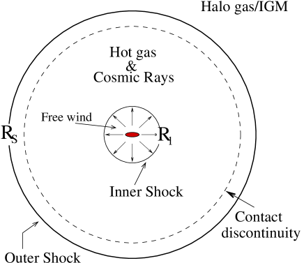
Figure 1: Wind profile for thermally and cosmic ray driven winds.

The evolution of such spherically symmetric outflows is governed by the following equations in the presence of cosmic rays and the hot gas (cf. Weaver et al., 1977; Ostriker & McKee, 1988; Tegmark et al., 1993),

$$\frac{{\rm d}^{2}R_{s}}{{\rm d}t^{2}} = \frac{4\pi R_{s}^{2}\left[P_{b}+P_{c}-P_{0}\right]}{m_{s}(R_{s})}-\frac{\dot{m}_{s}(R_{s})\left[\dot{R}_{s}-v_{0}(R_{s})\right]}{m_{s}(R_{s})}$$ (1)

$$\>\>\>\>\>\>\>-\frac{GM(R_{s})}{R_{s}^{2}},$$

$$\frac{{\rm d}}{{\rm d}t}\left[m_{s}(R_{s})\right]=\epsilon 4\pi R_{s}^{2}\rho_{B}(R_{s})\left[\dot{R}_{s}-v_{0}(R_{s})\right].$$ (2)

Here, the position of the outer shock is $R_{s}$, $m_{s}$ is the gas mass of the thin shell and $P_{b}$ and $P_{c}$ are the thermal and cosmic ray pressures in the hot bubble. Further, $\rho_{B}$ and $P_{0}$ are respectively the baryon density and the pressure of the outside medium assuming virial temperature for halo gas or $10^{4}$ K for the IGM; $v_{0}$ is the ambient velocity field taken from Furlanetto & Loeb (2001).

The first term in the right hand side of Eq. 1 represents the net pressure i.e. thermal plus cosmic ray pressure minus the outside pressure, that drives the outer shock. The second term is due to the mass loading of the shell from the outside medium causing the deceleration of the shock and we assume a fraction $\epsilon$ of all swept up mass remains in the thin shell (i.e. Eq. 2) and rest is mixed with the hot bubble due to evaporation/fragmentation (the mass in the hot bubble is negligible compare to the swept up mass). The 3rd term in Eq. 1 is the gravitational attraction due to the dark matter (a NFW profile is assumed with concentration parameter $c=4.8$, Navarro et al., 1997; Madau et al., 2001) as well as baryonic matter inside the radius $R_{s}$. For the initial baryonic density profile inside the halo we assume a beta model (Makino et al., 1998) and assume that a fraction, $f_{h}=0.1$ of total the total gas remains in the halo.

The thermal pressure $P_{b}$ can be obtained from the thermal energy of the bubble, $E_{b}$, by

$$P_{b}=\frac{E_{b}}{2\pi(R_{s}^{3}-R_{1}^{3})},$$ (3)

where we assume that the adiabatic index of the thermal gas $\gamma=5/3$. Here, $R_{1}$ is the position of the inner shock of the outflow. Similarly, the non-thermal cosmic ray pressure $P_{c}$ and the cosmic ray energy in the bubble, $E_{c}$, are related by,

$$P_{c}=\frac{U_{c}}{3}=\frac{E_{c}}{4\pi(R_{s}^{3}-R_{1}^{3})},$$ (4)

with the assumption that the adiabatic index of the CR component $\gamma_{CR}=4/3$ (considering them as highly relativistic particles). Here, $U_{c}$ is the energy density of the cosmic ray particles. The evolution of the thermal energy of the bubble is given by,

$$\frac{{\rm d}E_{b}}{{\rm d}t}=L(t)-\Lambda(t,T,Z)-4\pi\left[R_{s}^{2}\dot{R}_{s}-R_{1}^{2}\dot{R}_{1}\right]P_{b}.$$ (5)

The ‘free wind’ carries some fraction of total SNe energy in the host galaxy which is fed into the bubble as thermal energy, $L(t)$, at the inner shock. The bubble can lose its thermal energy due to $PdV$ work as it expands and radiative cooling. For cooling rate i.e. $\Lambda(t,T,Z)$, we consider Compton drag against the CMBR, bremsstrahlung and recombination line cooling that depends on temperature $T$ and metallicity, $Z$ of the gas. The gas density that determines the temperature of the hot bubble is taken to be the average density of the bubble. Note that the bubble is filled by the gas coming from the free wind and a fraction of the swept up mass. The free wind mass is higher for low mass galaxies owing to higher mass loading factor, $\eta_{w}$, that leads to higher radiative cooling of the bubble. Further, the metallicity of the bubble gas is self-consistently determined as described in the Appendix A of Paper I.

Similarly, the evolution of the cosmic ray energy in the bubble is governed by

$$\frac{{\rm d}E_{c}}{{\rm d}t}=L_{c}(t)-4\pi\left[R_{s}^{2}\dot{R}_{s}-R_{1}^{2}\dot{R}_{1}\right]P_{c}.$$ (6)

Here, $L_{c}$ is the total energy of the cosmic ray component per unit time injected into the bubble, at the inner shock. Note we consider, at the inner shock, the cosmic rays are being accelerated through diffusive shock acceleration with efficiency as high as 50% (Kang & Jones, 2003, 2005) in converting the kinetic energy of the shock front into cosmic rays. Thus, if initially we have 10% of total supernova energy available in the free wind, at the inner shock half of it will be available as thermal energy and rest half will be converted into cosmic ray energy. It is interesting to note that cosmic rays lose energy only due to adiabatic expansion that is solely determined from the outflow dynamics. But the thermal energy is lost by additional cooling processes and can be significant fraction of its initial energy. Thus, in case of only thermally driven wind one could encounter a situation where the gas has lost most of its thermal energy, the inner shock catches up with the outer shock and only the momentum of the free wind drives the outflow. This is known as ‘momentum driven outflow’ (see Samui et al., 2008, for evolution of such outflows). However, in the presence of non-zero cosmic ray energy, we will find that there is always a finite separation between the inner and outer shocks and hence the outflow never transits to the momentum driven case. Further, owing to a softer equation of state, cosmic rays lose energy slower than the thermal gas during adiabatic expansion. Hence even when radiative cooling of the bubble gas is efficient, cosmic ray pressure is important and moreover it dominates the outflow dynamics at the later stages of its evolution.

Most analytical models of galactic outflows do not consider the dynamics of the inner shock at $R_{1}$ (but see Paper I, ). We follow its dynamics using simply the jump condition across the inner shock boundary in a two fluid model assuming a strong shock. The evolution equation for $R_{1}$ is given by (Chevalier, 1983, and Appendix B)

$$P_{b}+P_{c}=\frac{2}{\gamma_{s}+1}\frac{\dot{M}_{w}(t_{e})}{4\pi R_{1}^{2}v_{w}}\left[v_{w}-\dot{R}_{1}\right]^{2},$$ (7)

with

$$\frac{2}{\gamma_{s}+1}=\frac{3\left(1+2\frac{P_{c}}{P_{b}}\right)}{4+7\frac{P_{c}}{P_{b}}}.$$ (8)

Here, $v_{w}$ is the asymptotic speed of the free wind material before it encounters the inner shock and related to the SNe energy by $L_{0}(t)=\dot{M}_{w}(t)v_{w}^{2}/2$, with the mass outflow rate $\dot{M}_{w}(t)$ is obtained from Eq. 24.

The mechanical luminosity, $L(t)$, and the cosmic ray luminosity at the inner shock, $L_{c}(t)$, fed into the wind bubble are related to the SNe explosion energy and hence the star formation rate of the host galaxy. Our model for calculating this star formation rate is described in Appendix A. It takes into account the negative feedback due to mass loss in the free wind following Samui (2014). However, we make some modifications that are needed in order to get a more accurate time resolved star formation rate in the low mass galaxies. The resulting evolution of the SFR for a few sample halo masses and collapse redshifts incorporating SNe feedback, are shown in Fig. 9, where we can see a significant suppression of the SFR for low mass galaxies. This model of star formation is similar in philosophy to the ‘bathtub model’ of Dekel et al. (2013) and Dekel & Mandelker (2014), applied however just after the formation of a new dark matter halo, either formed by mergers or from a collapsing density peak. Thus only the first burst of star formation lasting several halo dynamical time scale is considered. It does not consider the slow and continuous star formation mode of a galaxy that arises at a later stage of its evolution due to slow accretion process. Note that such a slow star formation may not result in an outflow that escapes the dark matter potential. We will explore such effects in future, but concentrate for now on the major epoch of star formation.

The luminosities $L(t)$ and $L_{c}(t)$ are related to the star formation rate $dM_{*}/dt$ by,

$$L(t)=10^{51}~{}{\rm ergs}\times\epsilon_{\rm w}~{}\nu~{}\frac{dM_{*}}{dt}$$ (9)

and

$$L_{c}(t)=10^{51}~{}{\rm ergs}\times\epsilon_{\rm cr}~{}\nu~{}\frac{dM_{*}}{dt}.$$ (10)

Here, we assume that $\nu$ number of SNe are formed per unit mass of star formation and each SNe produces $10^{51}$ ergs of energy on an average. A fraction of that energy, $\epsilon_{w}$ is channeled into the hot bubble as thermal energy and a fraction, $\epsilon_{\rm cr}$, is transformed in to the cosmic ray energy. In our model where the SNe first drives a free wind, which then flows into the hot bubble through a strong inner shock, it is this strong shock which reconverts the kinetic energy of the free wind back into both thermal energy and cosmic rays. Thus, the total energy efficiency in converting SNe energy to energy available for driving the outflow is $\epsilon_{w}+\epsilon_{\rm cr}$. For most of our calculations we assume $\epsilon_{w}=0.05$ and $\epsilon_{\rm cr}=0.05$ making total energy efficiency of 0.10. This efficiency is 2-3 times lower than the efficiency that has been found in numerical simulations (see Mori et al. (2002) where they obtained 20-30% efficiency) and hence a conservative value. Further, we assume a Salpeter initial mass function for the distribution of formed stars in the mass range $1-100$ M_⊙ that results in one SNe per 50 M_⊙ of star formation.

The above equations are simultaneously solved numerically starting from a set of initial conditions as described in Paper I. We follow the outflow dynamics till the outflow peculiar velocity decreases to the local sound speed in the IGM. At this point we assume that the shock would disappear and the outflowing material would mix with the IGM and expand with the Hubble flow.

3 Magnetic field dynamics

It is important to explore the magnetisation of the IGM by outflows. We have already mentioned that the magnetic fields play an important role in its interaction with cosmic rays and hence probably in the thermal history of the universe. Galactic outflows are potential candidates to magnetise the IGM. Here, we wish to get a conservative estimate of the strength of the IGM magnetic fields resulting from our outflow models. For simplicity, we treat evolution of magnetic fields separately and do not consider any dynamical effects of magnetic fields on the evolution of the outflow. Note that, adding the dynamical effect of magnetic fields can further aid in driving outflows. However, we have adopted a more conservative approach in present work as the magnetic pressure is always significantly subdominant to the CR pressure.

We assume that micro-Gauss level magnetic fields are present in the ISM of the high redshift protogalaxies when outflows begin. These fields themselves would be generated by turbulent dynamo processes in the galaxy (Brandenburg & Subramanian, 2005; Kulsrud & Zweibel, 2008; Ruzmaikin et al., 1988; Rodrigues et al., 2015). The ionised plasma in the wind would be coupled with this magnetic field and transport the magnetic flux out of the galaxy with the outflowing material. In order to calculate the strength of magnetic fields that can be deposited in the IGM via this process we follow Bertone et al. (2006) where they considered magnetising the IGM by thermally driven winds.

There are two possible scenarios in the co-evolution of magnetic fields and outflows. In the first case that we refer as ‘conservative’ model, the magnetic fields from galaxies are injected into the outflowing material and just get diluted as they expand with the outflow, obeying the magnetic flux freezing condition. The evolution of magnetic fields in such models is governed by following equation (Bertone et al., 2006),

$$\frac{dE_{B}}{dt}=\dot{E}_{B_{in}}-\frac{1}{3}\frac{\dot{V}_{w}}{V_{w}}E_{B}.$$ (11)

Here, $E_{B}$ is the total magnetic energy in the wind bubble; $V_{w}$ is the volume of the wind bubble. Further, $\dot{E}_{B_{in}}$ is the magnetic energy injection rate in the bubble from the galaxy and we take

$$\dot{E}_{B_{in}}=\epsilon_{B_{in}}\frac{\dot{M}_{w}}{\bar{\rho}_{in}}=\epsilon_{B_{in}}4\pi R_{1}^{2}v_{w}$$ (12)

with the density of the free wind material is given by

$$\bar{\rho}_{in}=\frac{\dot{M}_{w}}{4\pi R_{1}^{2}v_{w}}$$

and the magnetic energy density that is injected in the wind bubble is

$$\epsilon_{B_{in}}=\frac{B^{2}}{8\pi}\left(\frac{\bar{\rho}_{in}}{\bar{\rho}_{\rm ISM}}\right)^{4/3}.$$ (13)

$B$ is the magnetic field inside the star forming galaxy. The value of $B$ ranges from $\sim 10-20\mu$G in nearby spirals to values of $B\sim 50-100\mu$G in nearby starburst galaxies and in barred galaxies (see Beck, 2016, for a review and references). There is also tentative evidence from high-$z$ Mg ii system that $z\sim 1$ galaxies are already magnetized to current levels (Bernet et al., 2008; Farnes et al., 2014). Thus it seems reasonable to adopt $B\sim 10-20\mu$G for the galaxies at high redshift which are driving outflows. Further, $\rho_{\rm ISM}$ is the density of the ISM gas taken as 1000 times the average baryonic density of the halo.

In the above ‘conservative’ case we ignore the possible amplification of magnetic fields inside the outflow and thus we get the minimum possible value of magnetic fields that can be inputted into the IGM via outflows. In a more optimistic model B we take into account possible amplification of magnetic fields in the wind plasma due to shear flow and turbulence of the wind material. The characteristic time scale for this process is roughly given by (Bertone et al., 2006),

$$\tau_{\rm{eff}}^{-1}=f_{s}\frac{\dot{R}_{s}-H(t)R_{s}}{R_{s}}=f_{s}\left(\frac{\dot{R}_{s}}{R_{s}}-H(t)\right)$$ (14)

with $H(t)$ is the Hubble parameter. Here, $\dot{R}_{s}-H(t)R_{s}$ is the peculiar velocity of the outflow with respect to Hubble flow and dividing it by $R_{s}$ gives a measure of the velocity shearing rate in the outflowing material. Such a velocity could reflect itself in turbulence, which amplifies the field, due to a small-scale turbulent dynamo, on the turbulent eddy turn over timescales (Kazantsev, 1967; Brandenburg & Subramanian, 2005; Bhat & Subramanian, 2015). In such a dynamo the smallest eddy which has a magnetic Reynolds number above a critical value decides the rate of initial amplification. The fudge factor $f_{s}>1$ gives how much faster such an amplification occurs with respect to the shear time-scale. It will depend on the poorly known properties of the turbulence in the hot bubble and could be much greater than unity, if the smallest super critical eddy is much smaller than the bubble size. We assume $f_{s}\sim 1$ as a conservative estimate below. Including this amplification, the change in magnetic energy can be calculated from

$$\frac{dE_{B}}{dt}=\dot{E}_{B_{in}}+\left(\frac{1}{\tau_{\rm{eff}}}-\frac{1}{3}\frac{\dot{V}_{w}}{V_{w}}\right)E_{B}$$ (15)

which for $R_{s}\gg R_{1}$, can be simplified to

$$\frac{dE_{B}}{dt}=\dot{E}_{B_{in}}-H(t)E_{B}.$$ (16)

This would provide us a more optimistic value of the magnetic fields with which IGM can be seeded via outflows.

4 Structural characteristics of outflows

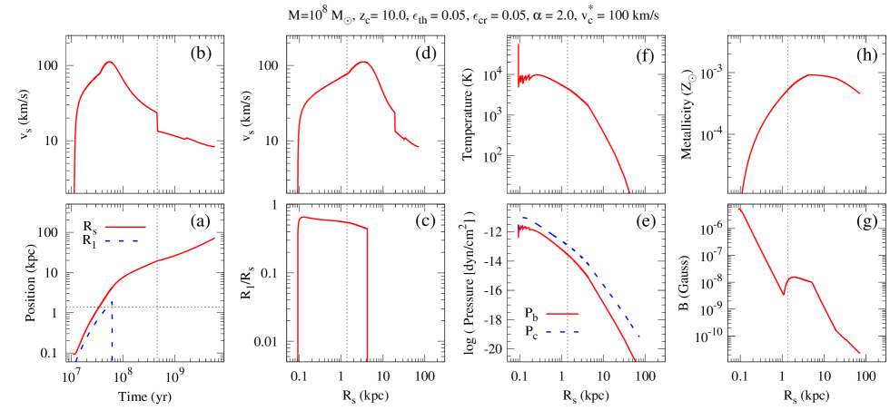
Figure 2: The characteristics of an outflow originating from a galaxy with total mass $M=10^{8}M_{\odot}$ that has collapsed at $z_{c}=10$. We show in panel (a) the position of inner ($R_{1}$) and outer shocks ($R_{s}$) as a function of time. In panels (b) and (d) we have shown the velocity of the outer shock as a function of time and its position ($R_{s}$) respectively. Panel (c) shows the ratio between the positions of inner and outer shocks as a function of $R_{s}$. The thermal and cosmic ray pressures as a function of $R_{s}$ are plotted in panel (e) with solid and dashed lines respectively. The evolution of the temperature and the metallicity of the hot bubble gas are shown in panels (f) and (h) respectively. In panel (g), the evolution of the magnetic field in the outflowing gas for our conservative model is plotted as a function of the outer shock position. The horizontal dotted line in panel (a) and vertical dotted lines in panels (c) to (h) mark the position of virial radius of the halo. The vertical dotted lines in panel (a) and (b) show the time when the outflow merges into Hubble flow.

Having set up the machinery for the evolution of outflows from star forming galaxies, driven by the thermal and non-thermal pressures and the spreading of magnetic fields and cosmic rays via such outflows, we present here some important characteristics of individual outflows resulting from our numerical calculations. We first focus on two representative masses of host galaxies in order to show the general trends in our models.

4.1 Outflow from dwarf galaxies

We begin with the study of outflows from a host galaxy of total mass $M=10^{8}$ M_⊙ that has collapsed at $z_{c}=10$. The star formation history of such galaxies is shown by the solid red curve in Fig 9. As we can see from this figure, in such small mass galaxies, due to strong negative SNe feedback or a large $\eta_{w}$, star formation completely stops after $10^{7}$ yrs. Hence, it is essential to investigate whether such strongly suppressed and brief duration of star formation can at all produce enough SNe energy to drive a galactic scale outflow from the galaxy. The important characteristics of the outflow originating from this particular galaxy are shown in Fig. 2. Indeed we see in Fig. 2 that a galactic scale outflow has resulted from such galaxy.

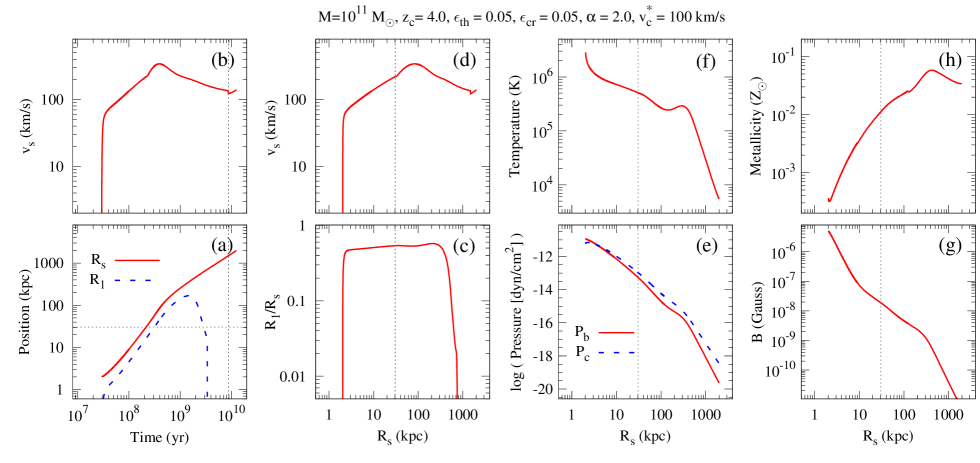
Figure 3: Same as Fig. 2 but for a halo of mass $M=10^{11}$ M_⊙ and collapse redshift $z_{c}=4$.

It is clear from panel (a) of Fig. 2, where we plot the location of inner and outer shocks as a function of time, that the outflow crosses the virial radius of the halo at $\sim 3\times 10^{7}$ yrs, goes far beyond the virial radius (shown by horizontal line) before it mixes with the IGM. The final physical radius of the outflow is 20 kpc before it is frozen into the Hubble flow after $\sim 3\times 10^{8}$ yrs from the collapse of the halo (as indicated by the vertical lines in panels (a) and (b) of Fig. 2). Note that the halo has a virial radius of 1.4 kpc. Therefore, the outflow originating from the host galaxy is able to pollute IGM with metals, magnetic fields and CRs upto $\sim 15$ times of its virial radius. The outflow achieves a maximum speed of 110 km/s just after crossing the virial radius of the halo (panel (b) and (d) of Fig. 2). The sudden increase in the velocity after crossing the virial radius is due to rapid change in the assumed gas density profile outside the halo.

It is interesting to note that even though star formation ceased after few times $10^{7}$ yrs the inner shock still persists upto a time $\sim 5\times 10^{7}$ yrs (panels (a) and (c)). This is due to the fact that it takes a finite time for the effects of energy release by SNe to be felt at the inner shock. The inner shock starts from the centre of the galaxy (our initial condition), rapidly goes closer to the outer shock reaching to a maximum of $0.65R_{s}$. Thus, it never comes very close to the thin shell and the outflow never transits to a momentum driven stage. It can be seen from panel (f) of Fig. 2 that the temperature of the bubble is always less than $10^{4}$ K. So in the absence of CRs, the thermal pressure alone would not have sustained the bubble region leading to a direct momentum impact of the free wind to the thin shell. However, in presence of cosmic ray pressure this never happens. At a very initial stage of the flow the thermal pressure and cosmic ray pressure were comparable to each other. But soon the gas loses its thermal energy by radiative cooling due to higher density of the wind material. At this point, the comic ray pressure becomes an order of magnitude higher than the thermal pressure even if initially they were of same order (see panel (e) of Fig. 2). This extra cosmic ray pressure completely governs the further evolution of the outflow keeping it always like an ‘energy driven flow’.

We now turn to the spreading of metals and magnetic fields by the outflow. Panel (g) of Fig. 2 shows the magnetic field strength in the outflowing gas, as a function of the outflow radius. Here, we have used the ‘conservative’ model for the magnetic fields evolution, and assumed $B\sim 10\mu$G in the galaxy. By the time outflow reaches the virial radius, the average strength of the magnetic fields is $\sim 0.02~{}\mu$G. It reduces farther reaching to a value of $0.4~{}$nano Gauss when the outflow mixes with the IGM. This field strength could be even larger if we take larger $B$ for the galactic field as would be appropriate for a star bursting galaxy. Note that the ‘optimistic’ model would predict an order of magnitude higher magnetic field strength. The implications of such fields will be discussed in Sec 6.2 and 6.3. The amount of metals carried by the wind material from the ISM to the bubble increases with time and hence it increases the metallicity of the bubble gas. We see from panel (h) that by this outflow we can pollute IGM with a metallicity of $Z\sim 0.001$ Z_⊙.

In a nutshell, the star formation and resulting SNe explosions in a $10^{8}$ M_⊙ halo can produce a galactic scale outflow of ‘cold’ gas, mostly driven by the cosmic ray pressure and can pollute a spherical region of radius 20 kpc (i.e. $\sim 15$ times the virial radius) with metals (metallicity of the polluted region is typically $\sim 0.001$ Z_⊙), cosmic rays and magnetic fields with of order a nano Gauss strength when it mixes with the IGM.

4.2 Outflow characteristic of a galactic scale halo

We now consider the outflow from a more massive halo with mass $M=10^{11}$ M_⊙ and collapse redshift of $z_{c}=4$. The outflow properties are shown in Fig. 3. We choose such an example as we will show later that these halos contribute most to the global volume filling of the wind material today. The basic picture remains the same as its low mass counterpart. However, there are certain differences. Owing to its higher star formation rate, the outflow from the halo extends to more than a Mpc from the centre of the galaxy before freezing into the Hubble flow (panel (a)). It achieves a maximum velocity of 340 km/s while crossing the virial radius of the halo (panel (b) and (d)). The outflow remains ‘energy driven’ through out its lifetime; the inner shock never catches up the outer shock as can be seen in panels (a) and (c) of Fig. 3.

The most striking difference between outflows from high and low mass galaxies is in the temperature evolution. In the low mass galaxy the outflowing material is cold. But in the high mass galaxy the density of hot bubble is low due to smaller $\eta_{w}$ making the radiative cooling less efficient. Thus as can be seen in panel (f) of Fig. 3, the temperature of the hot gas is more than $10^{6}$ K when the outflow starts. It decreases afterwards, but never becomes less than $10^{4}$ K when the outflow is in active stage. Further, the thermal and cosmic ray pressures remains comparable to each other through out the life time of the outflow (panel (e)). It is interesting to understand the evolution of both the pressures. Initially, the thermal pressure is higher than the cosmic ray pressure. However, after some time the cosmic ray pressure becomes higher. Such a feature arises due to different adiabatic indices for thermal gas and relativistic cosmic ray component causing pressure of the non-thermal component to decrease more slowly under adiabatic expansion (see Eqs. 3 and 4).

As can be seen from panel (h) of Figs. 2 & 3, $10^{11}$ M_⊙ halo spreads the metals over large distances and the resulting gas phase metallicity in the polluted region can be two orders of magnitude higher than that of a $10^{8}$ M_⊙ galaxy. The large galaxy produce more metals through SNe and thus eject more via outflow. On the other hand, they both magnetise the IGM with similar magnetic field strength but over different volumes. Thus outflows from massive galaxies pollute a fairly large volume of IGM with hot gas having higher metallicity. But they contribute in a similar fashion in magnetising the IGM. This may change if we consider a halo mass (or SFR) dependence in $B$ of Eq. 13.

Further, note that in panel (g) of Figs. 2 and 3, the evolution of the magnetic fields has been obtained for our ‘conservative’ models. The more ‘optimistic’ model B produces an order of magnitude higher magnetic field in the IGM. We will discuss its implication on the thermal history of IGM in section 6.2.

4.3 Comparison with Previous models

In this section we compare both cosmic ray and thermally driven outflows with models of Paper I that considered only the thermally driven outflows and a fixed mass loading factor $\eta_{w}=0.3$. As already mentioned, there are several improvements in present models compared to the model presented in Paper I. Firstly, the prescription for the star formation now takes into account the negative feedback arising from the SNe driven winds. Secondly, we also take into account the increased mass loading factor $\eta_{w}=(v_{c}/v_{c}^{*})^{-2}$ in small galaxies in the outflow dynamics as adopted in our star formation model. Finally, the winds are now driven by both thermal and cosmic ray pressures. As described before, the first two effects have opposite influence on the wind dynamics compared to the last one. In this section we compare different models in more detail.

In Fig. 4, we show the properties of thermally driven outflows with models discussed in Paper I by blue long dashed curves. The corresponding curves for models that includes SNe feedback, the increased mass loading but no effect of cosmic rays, are given in short dashed dark-green lines. In both the cases, we assume $\epsilon_{w}=0.1$ and $\epsilon_{\rm cr}=0$. The effect of the SNe feedback, increased mass loading, but now including the cosmic rays in the outflow dynamics keeping the total efficiency the same (i.e. $\epsilon_{w}+\epsilon_{\rm cr}=0.1$), is shown as red solid lines. The bottom panels consider outflow from a $10^{8}$ M_⊙ galaxy while the top panels are for $10^{11}$ M_⊙ halo. It is clear from the figure that the outflow escapes the low mass galaxy for the constant $\eta_{w}$ model of Paper I. However, including supernova feedback in star formation and increased $\eta_{w}$ prevent the outflow from taking off in such galaxies. This is reflected by the fact that the green short dashed curves are hardly noticeable in the first two columns of bottom panels of Fig. 4. This is because of (i) the reduction in the star formation (especially due to the larger $\eta_{w}$ in dwarf galaxies) and (ii) increase in the mass loading that leads to higher density and hence rapid cooling of the hot bubble gas. It is also evident from the figure that one can have outflows in such halos when we include the cosmic rays in the outflow dynamics (solid red curves) keeping the total energy efficiency the same. Thus we conclude that the presence of CRs enables outflows even in small mass galaxies with a large mass loading. Further, the outflowing gas will have low temperature due to efficient radiative cooling (temperature is $<10^{4}$ K as can be seen in the left bottom panel of Fig. 4).

For large galaxies with $M=10^{11}$ M_⊙, outflows do escape the dark matter potential in all three cases as described above. However, the cosmic ray driven outflows with same energy efficiency reaches much larger distance (see top panels of Fig. 4). This is because the cosmic ray pressure drops slower with radius than the thermal pressure due to a different adiabatic index. Thus cosmic ray pressure is able to push the outflowing gas further away compared to the one driven by thermally driven outflows. This can be seen from the velocity profile as plotted in the top middle panel of Fig. 4. Further, the temperature of the bubble gas is also lower by an order of magnitude in case of cosmic ray driven outflows making it more plausible for detection of metals.

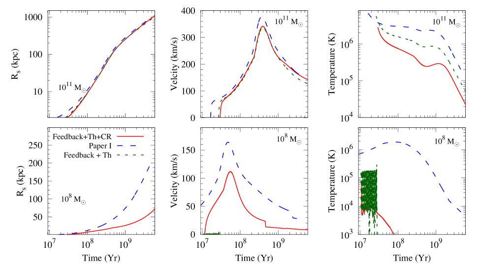
Figure 4: Comparison of old models of Paper I with new models for galaxies with masses $10^{8}$ M_⊙ (bottom panels) and $10^{11}$ M_⊙ (top panels). We show the outer shock positions (left panels), shock velocity (middle panels) and temperature of bubble gas (right panels) as a function of time. The solid red lines are for present models that consider SNe feedback in star formation and both cosmic rays and thermal gas drive outflows. Predictions by the models of Paper I that assumed only thermally driven outflows and did not take into account SNe feedback in star formation are shown by blue long dashed lines. Finally, outflows that are generated by only the hot thermal gas due to star formation with SNe feedback are shown by dark green short dashed lines.

5 Global influences of outflows

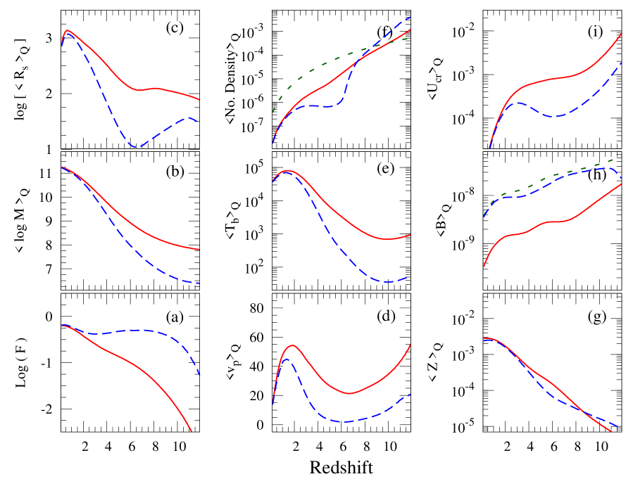
Figure 5: Global properties of outflows resulted from atomic cooling model (solid lines) and molecular cooling models (dashed lines). We show volume filling factor $F$ in panel (a). The porosity weighted average halo mass (in unit of M_⊙), outflow radius ($R_{s}$ in kpc), peculiar velocity ($v_{p}$ in km/s) and bubble gas temperature ($T_{b}$ in K) are shown in panels (b), (c), (d) and (e) respectively. In panel (f) we have compared the average number density per cc of the gas inside the bubble with the IGM number density density at that redshift (dotted curve). The amount of metals (in unit of Z_⊙) and magnetic fields in conservative models ($B$ in Gauss) that can be put in the IGM are shown in panel (g) and (h) respectively. Result for the optimistic models with molecular cooled halos is shown by dotted line in panel (h). Finally in panel (i) we show the excess cosmic ray energy density ($U_{cr}$ in eV/cm³).

In previous section we have investigated several key characteristics of outflows originating from the high redshift star forming galaxies. Here we show the global impact of outflows on the IGM at different redshifts. The most interesting physical quantity is the total volume of the universe/IGM that is affected/polluted by these outflows. In this respect we define volume filling factor as $F=1-\exp[-Q(z)]$ with porosity $Q$ is defined as

$$Q(z)=\int\limits_{M_{\rm low}}^{\infty}{\rm d}M\int\limits_{z}^{\infty}{\rm d}z^{\prime}\frac{{\rm d}^{2}N(M,z,z^{\prime})}{{\rm d}z^{\prime}{\rm d}M}\frac{4}{3}\pi\left[R_{S}(1+z)\right]^{3}.$$ (17)

Here, ${{\rm d}^{2}N(M,z,z^{\prime})}/{{\rm d}z^{\prime}{\rm d}M}$ is the comoving number density of dark matter halos having mass between $M$ and $M+{\rm d}M$ that are formed in redshifts range $z_{c}$ and $z_{c}+{\rm d}z_{c}$ and surviving till redshift $z$ without being merged with other halo. We use the modified Press-Schechter (PS) formalism of Sasaki (1994) to calculate this number density. In particular, it is obtained from (Chiu & Ostriker, 2000; Choudhury & Srianand, 2002; Samui et al., 2007)

$$\frac{{\rm d}^{2}N(M,z,z^{\prime})}{{\rm d}z^{\prime}{\rm d}M}~{}{\rm d}M~{}{\rm d}z^{\prime} = N_{M}(z^{\prime})\left(\frac{\delta_{c}}{D(z^{\prime})\sigma(M)}\right)^{2}\frac{\dot{D}(z^{\prime})}{D(z^{\prime})}\;$$ (18)

$$\times \frac{D(z^{\prime})}{D(z)}\frac{{\rm d}z^{\prime}}{H(z^{\prime})(1+z^{\prime})}~{}{\rm d}M.$$

Here, $N_{M}(z^{\prime}){\rm d}M$ is the Press-Schechter mass function (Press & Schechter, 1974), $\delta_{c}=1.686$ is the critical over density for collapse, $H(z)$ is the Hubble parameter, $D(z)$ the growth factor for linear perturbations and $\sigma(M)$ the rms mass fluctuation at a mass scale $M$.

Note that Eq. 18 does not take into account the survival of the hot bubble when two halos merge to form a bigger halo and thus using it in Eq. 17 would provide a lower limit on $Q$ or $F$. On the other hand if we use simple derivative of any mass function as the formation rate of halos and use it as ${{\rm d}^{2}N(M,z^{\prime})}/{{\rm d}z^{\prime}{\rm d}M}$, we would get an upper limit on the $F$ or $Q$ as we do not consider the merging of outflows. To explore this we use derivative of Sheth-Tormen mass function (Sheth & Tormen, 1999) to calculate the formation rate of halos and hence the volume filling factor and associated properties of outflows.

The lower mass limit ($M_{\rm low}$) in Eq. (17) is determined from the physical conditions required to host star formation. Before reionisation, gas inside a dark matter halo can cool via atomic hydrogen if virial temperature ($T_{\rm vir}$) of the halo is greater than $10^{4}$ K. In the presence of molecular hydrogen, a halo with virial temperature as low as 300 K can cool and host star formation (Tegmark et al., 1997; Haiman et al., 2000). In what follows we consider two models: (i) atomic cooled models where we assume $M_{\rm low}$ corresponds to $T_{\rm vir}=10^{4}$ K and (ii) molecular cooled models where we take $M_{\rm low}$ corresponds to $T_{\rm vir}=300$ K. Further, in the ionised regions of the universe due to radiative feedback, a halo can host star formation only if its circular velocity is more than about 35 km/s due to increase of Jeans mass (see Bromm & Loeb, 2002; Samui et al., 2008; Jose et al., 2014, for details of radiative feedback). Thus in order to know whether a halo can host star formation or not we need to follow the reionisation history of the universe self-consistently. We follow Samui et al. (2007) in order to calculate the ionisation state of the universe. At this point we wish to note that all our self-consistent reionisation models are compatible with available observations, namely reionization redshift $z_{re}\gtrsim 6$ and the resulting electron scattering optical depth is within $\tau_{e}=0.058\pm 0.012$ (Planck Collaboration et al., 2016b).

Further for any physical quantity related to outflows, we calculate porosity weighted average as

$$\langle X\rangle = Q^{-1}\int\limits_{M_{\rm low}}^{\infty}{\rm d}M\int\limits_{z}^{\infty}{\rm d}z^{\prime}~{}\frac{{\rm d}^{2}N(M,z,z^{\prime})}{{\rm d}z^{\prime}~{}{\rm d}M}\times$$ (19)

$$~{}~{}~{}~{}~{}~{}~{}~{}~{}~{}~{}~{}~{}~{}~{}~{}~{}~{}~{}~{}~{}~{}~{}~{}~{}~{}~{}\frac{4}{3}\pi\left[R_{S}(1+z)\right]^{3}X,$$

$X$ being the physical quantity. If one does not include $Q^{-1}$ factor it would correspond to the mean value of $X$ in the IGM.

5.1 Atomic cooling models

We start by showing results for our ‘atomic cooled’ models with Press-Schechter mass function. In Fig. 5 we show various physical quantities related to outflows as a function of redshift by solid curves. In panel (a) we show the most relevant quantity, the volume filling factor $F$ of the bubbles. Initially at $z=10$ the filling factor is small $\sim 0.01$, gradually increases to 0.26 at $z=3$ and finally reaches to 0.6 by $z=0$. Thus a minimum 60% of the universe can be filled with outflows from atomic cooled halos by today. The average halo mass contributing to the volume filling is plotted in panel (b). Above $z=6$ the average mass of haloes contributing most in volume filling is $\sim 10^{8}$ M_⊙. During this period the average bubble radius is 100 kpc (panel (c)). At later times both the average mass and bubble size increase slowly due to two reasons. Firstly, the number of higher mass galaxies are increasing in a hierarchical structure formation scenario. Secondly, the existing outflows are getting more time to grow in size. At $z=0$, massive galaxies with average mass $\sim 10^{11}$ M_⊙ having outflows of Mpc scale are responsible for polluting the IGM.

The porosity weighted peculiar velocity at different redshift is plotted in panel (d) of Fig. 5. Initially, most of outflows are in the early active stage having higher individual outflow velocity; thus the average peculiar velocity is also as high as 50 km/s. However, the outflows are coming from small mass galaxies. Hence they have a lower average temperature of $10^{3}$ K (see panel (e)). As the time passes, these outflows grow older and their speed reduces. But as new massive galaxies started collapsing, the peculiar velocity raises to 55 km/s at $z=2$. The average temperature of the bubble also shows a peak of $10^{5}$ K at the same time. The average density of the bubble is shown in panel (f) by the solid curve and most of the time it stays bellow the average IGM density (shown by the dashed line) at that redshift. This is expected as the hot bubble sweeps up the IGM into a shell creating a low density, high temperature regions.

In passing we note that several porosity weighted average physical quantities do not show monotonic behaviour with redshift such as porosity weighted peculiar velocity and radius of outflows. A number of counter veiling effects are responsible for such non-monotonic behaviour of the porosity weighted peculiar velocity ($v_{p}$). Although the characteristic mass of collapsing halos increases monotonically with decreasing redshift, the corresponding stellar to halo mass ratio is not monotonic with mass because of the reionization, supernovae and AGN feedbacks. Also as outflows expand, their velocity decreases, which is reflected by corresponding decrease in porosity weighted $v_{p}$ for $z>6$. Then after reionization, small mass halos lose their importance, more and more massive galaxies with younger outflows start to dominate and increase the average peculiar velocity till $z\sim 2$. After this star formation from very massive galaxies is being suppressed due to AGN feedback, while outflows from normal galaxies are becoming older, and the weighted $v_{p}$ decreases again.

One of the reasons for studying outflows is to understand how efficiently they can pollute IGM with heavier elements, magnetic fields and CRs. The metallicity and magnetic field evolution of the IGM are shown in the panels (g) and (h) of Fig. 5, respectively. As expected the IGM metallicity level increases with time as more and more SNe explode and resulting metals are put into the IGM via outflows. Finally, the metallicity of the IGM that can be reached by today is $\sim 10^{-2}$ Z_⊙ (panel (g)). Note that these metals are distributed in 60% volume of the universe. In the same volume, the average magnetic field strength that can be seeded by outflows is $0.4-4$ nano Gauss at $z=0-3$, for an assumed $B\sim 20\mu$G in galaxies, for our conservative model. Models with optimistic magnetic fields evolution predict, $\langle B\rangle\sim 2-20$ nano Gauss, or an order of magnitude higher magnetic fields seeded by this mechanism, as can be seen from the short dashed line of panel (h) in Fig. 5.

Finally, it is interesting to investigate the magnitude of the porosity weighted cosmic ray energy density that is still remaining in the plasma. We show this in panel (i) of Fig. 5. Before, $z=6$ the remaining CR energy density is as greater than $10^{-3}$ eV cm^-3. However, only 10% of the universe is filled with these cosmic rays. Even at low redshift the energy density of cosmic rays does not reduce much. At $z=3~{}(1)$ the excess energy density of in the cosmic rays is $5\times 10^{-4}$ eV cm^-3 ($10^{-4}$ eV cm^-3) in 26% (55%) volume of the universe. We will discuss this further in the following section and compare this energy density with the thermal energy density of the IGM.

We note that there is not much qualitative change in the globally averaged physical properties associated between our current model, where outflows are driven by both thermal and cosmic ray pressure, compared the models of Paper I, where we considered outflows to be only thermally driven. The crucial difference however, is that the current models have taken into account also the negative feedback on star formation due to SNe driven mass loss. One property which does change is the overall volume filling factor, which is smaller in the current models, compared to Paper I, because of the overall reduction in star formation due to SNe feedback. Further, the average temperature of the outflows has reduced dramatically, due to enhanced mass loading in the hot bubble, which will help in the detectability of the heavier elements in the quasar absorption spectrum.

5.2 Molecular cooled models

We now turn to the ‘molecular cooled’ models. As discussed in Paper I outflows from atomic cooled halos can potentially disturb Lyman-$\alpha$ forest due to their large peculiar velocity and higher temperature and we showed that molecular cooled halos provide a respite from this by filling the IGM at very early epoch with smaller outflows. Note that, in such small mass galaxies the mass loading factor $\eta_{w}$ is so high that the star formation ceases with the onset of supernova explosion, after $t_{\rm SNe}\sim 3\times 10^{7}$ yr. Within that period we find that in such galaxies the fraction of baryonic mass turned into stars (i.e. $M_{*}/M_{b}$) is of order 0.05 at $z=10$. Thus only about 5% of the baryons is converted to stars in such molecular cooled galaxies at high-$z$. Nevertheless, this does have a significant effect on the volume filling at high redshift. In Fig. 5 we show the global properties of outflows for such models with long dashed lines. As expected, in these models outflows volume filled quite early; at $z=8$, more than 75% of the IGM is filled by the wind material and hence with metals, cosmic rays and magnetic fields. The contribution comes mostly from galaxies of masses $10^{7}$ M_⊙ or less with average bubble size less than 30 kpc (see panels (b) and (c)). Upto $z=3$ the average peculiar velocity of the outflowing material is less than 20 km/s with average outflowing gas temperature less than $10^{4}$ K. Thus, cold gas from the small mass molecular cooled halos dominates the volume filling of the IGM and is expected not to disturb the Lyman-$\alpha$ forest. Note our results for molecular cooled halos will depend very much on the assumed value of $M_{*}/M_{b}$. This quantity is poorly constrained for such halos and some models suggest that it could be much less than what we assume here (Visbal et al., 2017). Understanding star formation efficiency in such low mass galaxies at early epoch is essential to accurately model their effect on global properties.

The other physical quantities such as gas density of bubbles, amount of metals and magnetic fields put in the IGM remain similar (panels (f), (g) and (h) of Fig. 5 respectively) in both molecular cooled and atomic cooled models. Note that in Fig. 5 we have shown the possible magnetisation of the IGM with our optimistic models as well and that resulted one order of magnitude higher value compared to conservative model. The excess porosity weighted cosmic ray energy density remains one order of magnitude smaller in case of molecular cooled models for $z\gtrsim 6$. After that the difference between atomic and molecular cooled models decreases and finally by $z\lesssim 2$ they become equal.

5.3 Effect of mass function and formation rates

Here, we show effects of different halo mass functions on global properties of outflows. In Fig. 6 we compare the porosity and the volume filling factor as obtained from using Sheth-Tormen (ST) mass function with that of Press-Schechter (PS) mass function. From the figure it is clear that the Sheth-Tormen mass function predicts a much larger volume filling of the universe. For example in atomic cooled models at $z=3$, the ST mass function predicts 60% volume of the universe is filled with outflows (red dotted-dashed curve) compared to 35% with PS mass function (solid blue curve). Similarly for molecular cooled models at $z=3$, the volume filling factors are $F=0.65$ and 0.41 for ST and PS mass function respectively. Note that other physical properties do not change much when using different prescription for the halo formation rate.

It is interesting to note that when we use the Sasaki formalism to calculate the formation rate of halos and include molecular cooled halos, the porosity decreases at $z\sim 6$ before increasing again at $z\sim 2$. In the Sasaki formalism, one has a survival probability for a halo collapsing at redshift $z_{c}$ to survive till a later redshift $z$ (Sasaki, 1994). However when a halo is destroyed by merging to form a bigger halo, its outflow will survive, if it has gone far beyond the virial radius. Such outflows are not easy to take into account in a semi-analytical model such as ours, and we have neglected their contribution to the porosity. This can lead to a decrease in the volume filling factor. This effect is important when one calculates the volume filling factor of outflows from molecular cooled halos which collapse at high-$z$, before reionization. On the other hand, models considering derivative of any mass function would over estimate the volume filling factor by considering outflows separately from halos after and before merging (Samui et al., 2009a). Thus calculations which employ the formation rate using the Press-Schechter-Sasaki formalism and Sheth-Tormen-derivative bracket the expected behavior of volume filing factor, which is why we have considered both of them in the present work. Further, in Samui et al. (2009a) we have tested the sensitivity of the porosity not only for various mass functions but also to different prescriptions for the formation rate of halos. It was shown that the filling factor as well as other physical quantities were reasonably insensitive to changes in the mass function.

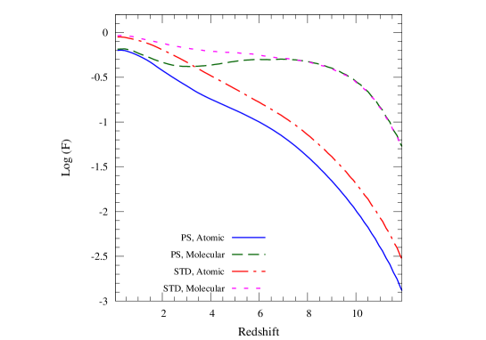
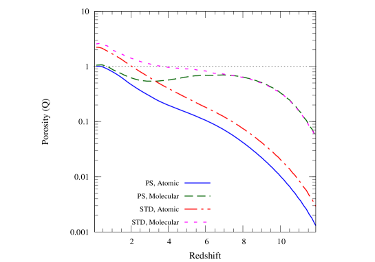
Figure 6: Comparison of volume filling factor (top panel) and porosity (bottom panel) as expected from different mass functions. Solid blue line and red dotted-dashed line show the filling factor predicted by atomic cooled models with PS and ST mass functions respectively. For molecular cooled models the comparison is shown by green dashed (PS) and magenta dotted (ST) lines.

Thus we conclude that outflows can significantly volume fill the universe with metals, magnetic fields and cosmic rays. In passing we note that Bertone et al. (2006) also got similar magnetic field strength of $10^{-8}-10^{-12}$ Gauss in the IGM. However, their outflows never volume filled the universe as their simulation did not include small mass galaxies.

6 Implications of outflow models

The outflow models discussed here has a number of interesting consequences, which we discuss below.

6.1 Detectability of metals

In Paper I, we discussed the detectability of low density high temperature outflowing material in the presence of meta-galactic UV background through O vi and C iv absorption lines (see section 7 of Paper I, ). In particular, we focused on absorption signatures that could arise from (i) the free wind, (ii) hot bubble and (iii) gas in the shell. The main difference in our current work is that, in the case of low mass halos the mass loading is higher and in the case of high mass halos the bubble temperature is lower when we include the CRs. Moreover, we are also considering magnetised outflowing material in the current work. Here we discuss the possible consequences without going into detailed radiative transport modelling.

In Paper I, it was suggested that the low ion absorption seen through Mg ii, Na i and Ca ii transitions can not be produced in the free winds and could originate from multiphase structure likely to form inside the outflow due to (i) cold gas ejected from the galaxy along with the free wind, (ii) dense cloud formed from the Rayleigh-Taylor instability of the swept up shell or (iii) cold gas clumps formed due to cooling instabilities etc.

We first ask, can the free wind driven by CR discussed here be detected in Mg ii absorption. In Fig.7 we show the total integrated hydrogen column density produced by the free wind as a function of time for a halo of mass $10^{11}$ M_⊙. The integrated column density of total hydrogen inferred is very similar to what we had for models discussed in Paper I. All the discussions presented there is applicable here as well. In particular, to produce low ion absorption lines, we need multiphase structure with cold clumps originating from the above mentioned possibilities in addition to the flow structure discussed in this work.

Next we consider the survivability of such cold clouds in the outflow. As discussed in Paper I, the evaporation time-scale goes as $T^{-5/2}$. As can be seen in Fig. 4, the bubble temperature in our present models are typically factor 4 times smaller than for models considered in Paper I. This alone makes the evaporation time-scale $\sim 32$ times longer than what we inferred for the pure thermally driven model without any feedback. Even when we consider the SNe feedback inclusion of CRs increases the evaporation time-scale by a factor 5. This suggests that survival of cold dense clumps in the outflow can be relatively easier in our models with CR driven flows. Further, in a magnetised outflow, magnetic fields can drape themselves around a gas cloud, and reduce evaporation of gas across the field even further.

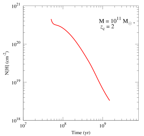
Figure 7: Hydrogen column density in the free wind for a halo of mass $10^{11}$ M_⊙. It is shown till the star formation lasts.

6.2 Thermal history of the IGM

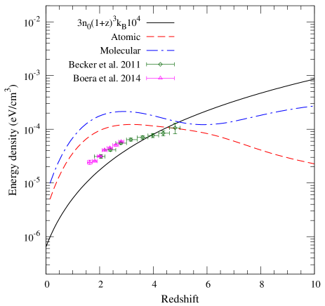
Figure 8: The thermal energy density of the ionised IGM at mean IGM density with a temperature $10^{4}$ K is shown by the solid line. In comparison, we show the porosity weighted energy density of the cosmic rays as expected from our atomic cooled models (dashed line) and molecular cooled models (dotted-dashed line). Further, the data points with error bar are the energy density of the IGM assuming the temperature of the IGM as measured by Becker et al. (2011) (open diamonds) and Boera et al. (2014) (filled triangles).

We now explore the possible implications of the excess cosmic ray energy from outflows to the thermal history of the IGM. As noted earlier, observations of absorption lines in high redshift quasar spectra reveal that the temperature of the IGM at $z=2-3$ is few times $10^{4}$ K (Becker et al., 2011). This temperature is measured in the mildly overdense regions of the IGM with overdensity less than 10 as probed by the Lyman-$\alpha$ forest. It is believed that the IGM temperature keeps some memory of the reionisation process at high-$z$. At the end of the hydrogen reionisation the temperature of the IGM is set to $1-3\times 10^{4}$ K (Schaye et al., 2000; Ricotti et al., 2000) due to photoionisation heating. In absence of any other heating mechanism after reionisation, the IGM temperature should drop adiabatically with the expansion of the universe as $(1+z)^{2}$. Thus in models where reionization of the universe occurred earlier than $z=6$ (as expected from observations of quasar spectra) one would not be able to explain the observed IGM temperature at $z=2-3$. We need an additional heating mechanism to explain this temperature floor. Several authors have suggested the late HeII to HeIII reionisation by the harder quasar spectrum as the reason for this excess temperature (Furlanetto & Oh, 2008; Bolton et al., 2009). Here we discuss if excess CR energy from outflows can heat the IGM at $z=2$ to 3.

Note that wherever galactic outflows percolate, they carry magnetic fields and cosmic rays in addition to metals. Thus, say at $z=3$ for models assuming PS mass function, 50% of the universe is filled by the outflows from molecular cooled halos (35% for atomic cooled model) with $\sim 10$ nano Gauss magnetic fields (optimistic model) and excess average cosmic ray energy density of $10^{-4}$ eV/cm³. With ST mass function for atomic and molecular cooled models, respectively 65% and 41% of the universe is filled with outflows and similar amount of magnetic fields and excess average cosmic ray energy density. Note that in standard model of structure formation, the outflow affected regions are expected to collapse to form filamentary structures at latter stages that are likely to be detected as Lyman-$\alpha$ forests in the quasar spectrum. The cosmic ray particles (protons) gyrate along the magnetic fields lines and generate Alfvén waves by a streaming instability (Kulsrud & Pearce, 1969; Kulsrud, 2004). These waves damp out and transfer energy to the thermal gas. The rate of energy transfer to the gas via the Alfvén waves is given by $|v_{A}.\nabla P_{c}|$ where $v_{A}=B/\sqrt{4\pi\rho}$ is the Alfv́en velocity ($\rho$ is the density of plasma) (Wentzel, 1971). The modulus is taken as in this process CRs always lose energy. Note that for ionised gas with temperature $T$ the thermal energy density is given by $E_{th}=3n_{H}k_{B}T$, $n_{H}$ being the number density of hydrogen and $k_{B}$ is the Boltzmann constant. Thus, time taken to deposit cosmic ray energy of the order of thermal energy is given by,

$$t_{cr}=\dfrac{3nk_{B}T}{|v_{A}.\nabla P_{c}|}.$$

Comparing this with the Hubble time $t_{H}$ at a given epoch we get,

$$\dfrac{t_{cr}}{t_{H}}=H(z)\dfrac{3nk_{B}T}{|v_{A}.\nabla P_{c}|}.$$

Putting in numbers we find,

$$\dfrac{t_{cr}}{t_{H}}\approx 0.3\left(\dfrac{h}{0.7}\right)^{4}\left(\dfrac{\Omega_{m}}{0.3}\right)^{1/2}\left(\dfrac{1+z}{4}\right)^{6}\left(\dfrac{T_{4}}{B_{10{\rm nG}}}\right)$$

$$\times\left(\dfrac{3\times 10^{-4}{\rm eV/cm}^{3}}{U_{cr}}\right)\left(\dfrac{L}{0.1~{}{\rm Mpc}}\right).$$ (20)

Here, $T_{4}$ is the temperature in the unit of $10^{4}$ K and $B_{10{\rm nG}}$ is the magnetic field in unit of 10 nano Gauss. Further we have normalised this ratio assuming a typical pressure gradient scale of a filament is $L\sim 0.1$ Mpc (Schaye, 2001) and cosmic ray energy density $U_{cr}=3\times 10^{-4}$ eV/cm³. Hence, if the IGM at $z=3$, has been polluted by outflows with $B$ of 10 nano Gauss and $U_{cr}=3\times 10^{-4}$ eV/cm³, within 1/3rd of the Hubble time, the CRs would dissipate energy to the thermal gas via Alfvén waves, increasing IGM temperature to $10^{4}$ K. For even lower redshift, the process is more efficient.

In Fig. 8 we have plotted the volume average cosmic ray energy density available from our outflow models and compared it with the thermal energy of the ionised IGM of temperature $10^{4}$ K. We have also shown thermal energy of the Lyman-$\alpha$ forests with temperatures as measured by Becker et al. (2011) and Boera et al. (2014). It is clear that the average cosmic ray energy density around $z\sim 3$ ($U_{cr}\sim 10^{-4}$ eV/cm³) is much higher than the thermal energy density of the IGM with temperature $10^{4}$ K, especially for molecular cooled models. The porosity weighted CR energy density would be even higher. In the mildly overdense regions of the IGM which produce Lyman-$\alpha$ forest $U_{cr}$ can be enhanced further by adiabatic compression to few times $10^{-4}$ eV/cm³. Magnetic field will also be enhanced due to flux freezing to few tens of nano Gauss. Thus one can see from Eq. 20, that CRs can transfer sufficient energy to the thermal gas within the Hubble time and potentially heat the IGM around $z=2-4$ to a temperature of $\sim 10^{4}$ K to erase the thermal signature of reionization. This conclusion would be more appropriate for molecular cooled models where outflows volume filled the universe early in time.

Note that here we have considered CRs that are accelerated in the inner shocks only. However, we have not considered the CRs that can be generated in the terminal shock of the outflows as well as in the structure formation shocks. Simulations predict cosmic ray energy density of $\sim 10^{-5}$ eV/cm³ that can arise from structure formation shocks with Mach number of few tens (Jubelgas et al., 2008; Pfrommer et al., 2017). Adding these sources of cosmic rays would lead to more efficient heating of the IGM by cosmic rays.

6.3 IGM magnetic fields

As noted earlier, $\gamma$-ray observation of nearby blazars (with $z\sim 0.1-0.2$), have tentatively indicated a lower limit for magnetic fields in voids, $B_{V}\sim 10^{-16}$ Gauss provided their coherence length $l_{B}$ greater than about a Mpc (Neronov & Vovk, 2010; Tavecchio et al., 2011). For fields with much smaller coherence scale, the lower limit increases as $l_{B}^{-1/2}$ with decreasing $l_{B}$. There fields in voids could be primordial arising from processes in the early universe (Durrer & Neronov, 2013; Subramanian, 2016, for review).

However, by such low redshifts, all our models predict a porosity of wind material greater than unity or volume filling factor greater than 0.6 for randomly distributed sources. This implies that outflows could have percolated even in the void regions by the present epoch. Further the porosity averaged value of the magnetic fields in our models are $\sim$ nano Gauss, and the radius of the outflowing bubbles is of order Mpc. The coherence scale of the fields could be smaller than this radius due to turbulent tangling. And the field strength could be diluted further in outflows frozen into the expanding IGM in voids. Nevertheless, the field strength in our models are sufficiently large compared to $B_{V}$, that it is highly likely that they satisfy the constraints set by the $\gamma$-ray observations. Thus magnetic fields inferred in the voids or in general IGM need not be of primordial origin. Rather they could be of astrophysical origin, generated/amplified in the star forming galaxies and transported from there to the IGM by the outflows created from the supernova explosions. One caveat is that large-scale clustering could result in a smaller volume filling of outflows in the void regions. It would be of interest to therefore consider our outflow models in more detail, in biased proto-void regions.

7 Discussion and Conclusions

In the present work, we have explored how cosmic rays could aid in driving relatively cold outflows from high redshift galaxies, and resulting global consequences. The primary sources of energy for outflows are SNe in the high-$z$ galaxies, and a fraction of this energy goes into cosmic rays. Outflows also cause a negative feedback on the star formation rate in a galaxy which can be especially large in low mass galaxies. We show that even with such suppression, low mass galaxies can still drive an outflow in the presence of cosmic rays.

Cosmic rays are accelerated in the SNe shocks and produce cold free winds upto the inner shock and are then re-accelerated there. These cosmic rays add extra pressure to the thermal gas that can even drive a cold outflow. We find that outflows extend to tens of kpc in dwarf galaxies with halo mass $\sim 10^{8}$ M_⊙ before merging with cosmological expansion, whereas massive galaxies with halo of masses $10^{11}$ M_⊙ have Mpc scale outflows. Cosmic ray driven outflows can go to a larger radii compare to a purely thermally driven outflow with same total energy input. This is because the cosmic ray pressure decreases less rapidly compared to the thermal pressure with adiabatic expansion (due to its softer equation of state) and comes to dominate outflow dynamics at large radii.

We showed that these outflows could significantly volume fill the universe with metals, magnetic field and excess cosmic rays. In particular, at $z=3$ for the ST mass function with molecular cooled halos, 65% of the universe is filled with the outflowing gas along with metals, magnetic fields of order $10^{-8}$ G and excess cosmic ray energy density of $\sim 10^{-4}$ eV/cm³. All our models predict a volume filling factor of order unity by $z\sim 0$.

Further, we explore three implications of such outflows. We argued that due to lower temperature and higher density of the free wind as well as the bubble gas, the metals spread by the outflow could be more easily detected as absorption line system. Low ionisation metals such as Na i or Mg ii are likely to be detected in gas clouds embedded the free wind, whereas others like C iv or O vi would come from the bubble or from pre-enriched IGM. Moreover, we showed that the excess energy density in cosmic rays from these outflows could be transferred efficiently enough to the thermal IGM gas in presence of magnetic fields. This can potentially erase the thermal history of reionisation and heat the IGM to a temperature of order $10^{4}$ K as inferred from quasar spectra. Finally, we find that void magnetic fields of order $10^{-16}$ G as inferred from blazar observation, need not be of primordial origin, but could be of astrophysical origin generated in star forming galaxies and transported by the cosmic ray driven winds to the voids.

Our models which estimate the global impact of outflows on the IGM, at present do not take account of spatial clustering of galaxies. In order to have more realistic scenario, it would be of interests to put the cosmic ray driven outflows in numerical simulation of structure formation.

Appendix A Star formation model with supernova feedback

In Samui (2014), we discussed star formation models incorporating supernova feedback that are constrained by observations of UV luminosity functions of Lyman-break galaxies in the redshift range $1.5-10$ and the correlations found between star formation rate (SFR), stellar mass and gas phase metallicity. Here, we broadly follow the same prescriptions with some modifications that are needed in order to get more accurate time resolved star formation rate in the low mass galaxies that are likely to be important in spreading metals into the IGM.

Consider a dark matter halo of mass $M$ which virialises at redshift $z_{c}$ and starts to accrete baryonic mass $M_{g}(t)$. A total fraction, $f_{*}$, of the accreted gas is assumed to be in the cold phase and available for star formation. At a given time a portion of this cold gas is locked up in low mass stars formed from previous episodes of star formation. Further, massive stars explode as supernova after a characteristic life time of $t_{\rm SNe}\sim 10^{7}$ yrs, and inject energy and momentum to the surrounding gas. A fraction of cold gas will then leave the galaxy making it unavailable for subsequent star formation.

Taking these processes in to account, and assuming that the instantaneous star formation rate, $dM_{*}(t)/dt$, of a galaxy is proportional to its cold gas content, we have

$$\frac{dM_{*}(t)}{dt}=f_{t}\left[\frac{f_{*}M_{g}(t)-M_{*}(t)-M_{w}(t)}{\tau}\right].$$ (21)

Here $\tau$ is the dynamical time scale for the halo and $f_{t}$ governs the duration of star formation activity in terms of this time scale. Further $M_{*}(t)$ is the stellar mass at any time $t$, $M_{w}(t)$ is the mass of cold gas lost in the wind and the numerator of Eq. 21 reflects the cold gas mass still available for star formation. The time derivative of Eq. 21 leads to

$$\frac{d^{2}M_{*}(t)}{dt^{2}}=\frac{f_{t}}{\tau}\left[f_{*}\frac{dM_{g}(t)}{dt}-\frac{dM_{*}(t)}{dt}-\frac{dM_{w}(t)}{dt}\right].$$ (22)

In order to solve for the star formation rate one needs to specify both baryonic accretion rate and the mass loss rate of cold gas in the outflow.

We assume that the baryon accretion rate in the central part of galaxy, a time $t$ after halo formation, goes as

$$\frac{dM_{g}}{dt}=\left(\frac{M_{b}}{\tau}\right)e^{-\frac{t}{\tau}}.$$ (23)

Here $M_{b}$ is the total baryonic mass that would be accreted in the halo and the characteristics time scale for accretion is taken to be the dynamical time scale for the halo.

The mass outflow rate due to SNe explosion at time $t$ is assumed proportional to the star formation rate at an earlier time $(t-t_{\rm SNe})$ (to take account of the delay between star formation and resulting supernovae), i.e.,

$$\dot{M}_{w}(t)=\eta_{w}\dot{M}_{*}(t-t_{\rm SNe}).$$ (24)

where over dot represents the time derivative. Depending on the actual mechanism of the outflow, the proportionality constant $\eta_{w}$ is either $\propto v_{c}^{-2}$ (energy driven/ cosmic ray driven outflows) or $\propto v_{c}^{-1}$ (momentum driven outflows) ; $v_{c}$ being the circular velocity of the dark matter halo hosting the galaxy. Further, we showed in Samui (2014) that a $\eta_{w}\propto v_{c}^{-2}$ is consistent with the amount of stellar mass detected in low mass dwarf galaxies. We also show that in presence of cosmic rays, the outflow never transits to a momentum driven stage. Note that we will use the notation $\eta_{w}=(v_{c}/v_{c}^{*})^{-\alpha}$ with $v_{c}^{*}$ fixing the normalisation and different values of $\alpha$ indicating the type of outflow.

Using Eq. 23 and Eq. 24 in Eq. 22 then gives

$$\frac{d^{2}M_{*}(t)}{dt^{2}}=\frac{f_{t}}{\tau}\left[f_{*}\frac{M_{b}}{\tau}e^{-\frac{t}{\tau}}-\frac{dM_{*}(t)}{dt}-\eta_{w}\frac{dM_{*}(t-t_{\rm SNe})}{dt}\right].$$ (25)

Note the explicit $t$ dependence here. This is only true for $t>t_{\rm SNe}$. For $t\leq t_{\rm SNe}$ we have no supernova feedback and then,

$$\frac{d^{2}M_{*}(t)}{dt^{2}}=\frac{f_{t}}{\tau}\left[f_{*}\frac{M_{b}}{\tau}e^{-\frac{t}{\tau}}-\frac{dM_{*}(t)}{dt}\right].$$ (26)

In order to follow the star formation rate of individual galaxies for $t>t_{\rm SNe}$, we solve the delayed differential equation (Eq. 25) numerically. For $t<t_{\rm SNe}$, one can integrate Eq. 26 analytically with the boundary condition that $dM_{*}/dt=0$ at $t=0$ and get

$$\frac{dM_{*}}{dt}=\frac{M_{b}f_{*}f_{t}}{\tau[f_{t}-1]}\Bigg{[}e^{-\frac{t}{\tau}}-e^{-f_{t}\frac{t}{\tau}}\Bigg{]}.$$ (27)

Further, for simplicity we assume $f_{t}=1$ (as in Samui, 2014) and therefore

$$\dot{M}_{*}(t) = \frac{f_{*}M_{b}}{\tau}\frac{t}{\tau}\exp\left[-\frac{t}{\tau}\right].$$ (28)

for $t<t_{\rm SNe}$. This evaluated at $t=t_{\rm SNe}$, also provides the initial condition for the numerical solution of Eq. 25.

In Fig. 9 we show the resulting star formation rate of few example galaxies with $\alpha=2$ and $v_{c}^{*}=100$ km/s. Further, we assume $f_{*}=0.5$. Note this $f_{*}$ is not what is canonically referred to as the star formation efficiency in literature. Rather, the total fraction of baryons converted to stars in a galaxy over its lifetime would be $f_{*}/(1+\eta_{w})$. These representative samples are chosen to show a range in the time evolution of the star formation rate that can be envisaged in our models. For very low mass galaxies such as the one with $M=10^{8}~{}M_{\odot}$, we see a complete suppression of star formation once the wind starts after $t_{\rm SNe}$ (solid red curve). In these galaxies the mass outflowing rate or $\eta_{w}$ is very high. The star formation which happens within $t_{\rm SNe}$ is enough to eject rest of the gas from the shallow dark matter potential quenching further star formation completely. Galaxies with slightly larger masses ($M=5\times 10^{8}~{}M_{\odot}$) show periodic/episodic star formation activity (dashed blue curve). While $\eta_{w}$ is not high enough to suppress the star formation completely, it definitely lowers the star formation that causes a reduction in subsequent mass outflow as well. This in turns increases the gas reservoir and hence the star formation, resulting a oscillating star formation mode in the galaxy. Note that these two modes of star formation i.e. complete suppression and episodic star formation would not have been seen in our model unless we consider the delay of $t_{\rm SNe}$ between star formation and onset of outflows.

Larger mass galaxies ($M=10^{9}~{}M_{\odot}$) do not show such oscillations in star formation but suppression due to outflows is clearly noticeable (magenta dotted-dashed curve in Fig. 9). For very massive galaxies (i.e. $M\gtrsim 10^{11}~{}M_{\odot}$), there is negligible suppression of star formation. Due to deeper gravitational potential, the mass outflow rate is small in those galaxies, hence there is no strong suppression of star formation due to the wind feedback. Note that we only consider $\alpha=2$ as we will show later that the outflows would never be going to a momentum driven case in presence of cosmic rays. Also the normalisation circular velocity $v_{c}^{*}=100$ km/s is chosen because it reproduces various observations regarding high redshift universe (see Samui, 2014). These star formation models are used to calculate the outflow properties in the main text.

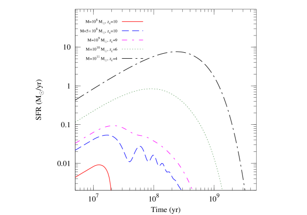
Figure 9: Time evolution of SFR for different galaxies; The halo mass ($M$) and the collapsed redshift ($z_{c}$) are marked in the legends. We have assumed $\alpha=2,~{}v_{c}^{*}=100$ km/s.

Appendix B Shock jump conditions in presence of cosmic rays

The shock jump conditions of two fluid models with one relativistic component ($\gamma=4/3$) and one non-relativistic component ($\gamma=5/3$) were evaluated by Chevalier (1983). They are (Eqn. 5 to 8 of Chevalier, 1983),

$$\rho_{2} = \dfrac{\gamma_{s}+1}{\gamma_{s}-1}\rho_{1}$$ (29)

$$v_{2} = \dot{R}_{1}+\dfrac{\gamma_{s}-1}{\gamma_{s}+1}\left(v_{w}-\dot{R}_{1}\right)$$ (30)

$$P_{b} = \dfrac{2(1-w)}{\gamma_{s}+1}\rho_{1}\left(\dot{R}_{1}-v_{w}\right)^{2}$$ (31)

$$P_{c} = \dfrac{2w}{\gamma_{s}+1}\rho_{1}\left(\dot{R}_{1}-v_{w}\right)^{2}$$ (32)

$$\gamma_{s} = \dfrac{5+3w}{3(1+w)},$$ (33)

with $w=P_{c}/(P_{c}+P_{b})$. Here, subscript 1 and 2 are for pre-shocked and post-shocked properties respectively. Further, we assume that $w$ remains constant across the shock. Adding, Eqn. 31 and Eqn. 32 we obtain Eq. 7. Putting $w$ explicitly in terms of $P_{c}$ and $P_{b}$ one can get Eq. 8.

References

- Beck (2016) Beck R., 2016, A&A Rev., 24, 4
- Becker et al. (2011) Becker G. D., Bolton J. S., Haehnelt M. G., Sargent W. L. W., 2011, MNRAS, 410, 1096
- Bell (2015) Bell A. R., 2015, MNRAS, 447, 2224
- Bernet et al. (2008) Bernet M. L., Miniati F., Lilly S. J., Kronberg P. P., Dessauges-Zavadsky M., 2008, Nature, 454, 302
- Bertone et al. (2006) Bertone S., Vogt C., Enßlin T., 2006, MNRAS, 370, 319
- Bhat & Subramanian (2015) Bhat P., Subramanian K., 2015, Journal of Plasma Physics, 81, 395810502
- Boera et al. (2014) Boera E., Murphy M. T., Becker G. D., Bolton J. S., 2014, MNRAS, 441, 1916
- Bolton et al. (2009) Bolton J. S., Oh S. P., Furlanetto S. R., 2009, MNRAS, 395, 736
- Brandenburg & Subramanian (2005) Brandenburg A., Subramanian K., 2005, Phys. Rep., 417, 1
- Breitschwerdt et al. (1991) Breitschwerdt D., McKenzie J. F., Voelk H. J., 1991, A&A, 245, 79
- Bromm & Loeb (2002) Bromm V., Loeb A., 2002, ApJ, 575, 111
- Carswell et al. (2002) Carswell B., Schaye J., Kim T.-S., 2002, ApJ, 578, 43
- Chen et al. (2010) Chen H.-W., Helsby J. E., Gauthier J.-R., Shectman S. A., Thompson I. B., Tinker J. L., 2010, ApJ, 714, 1521
- Chevalier (1983) Chevalier R. A., 1983, ApJ, 272, 765
- Chevalier & Clegg (1985) Chevalier R. A., Clegg A. W., 1985, Nature, 317, 44
- Chiu & Ostriker (2000) Chiu W. A., Ostriker J. P., 2000, ApJ, 534, 507
- Choudhury & Srianand (2002) Choudhury T. R., Srianand R., 2002, MNRAS, 336, L27
- Cooksey et al. (2013) Cooksey K. L., Kao M. M., Simcoe R. A., O’Meara J. M., Prochaska J. X., 2013, ApJ, 763, 37
- D’Odorico et al. (2013) D’Odorico V., et al., 2013, MNRAS, 435, 1198
- D’Odorico et al. (2016) D’Odorico V., et al., 2016, MNRAS, 463, 2690
- Davé et al. (2008) Davé R., Oppenheimer B. D., Sivanandam S., 2008, MNRAS, 391, 110
- Davé et al. (2011) Davé R., Oppenheimer B. D., Finlator K., 2011, MNRAS, 415, 11
- Dekel & Mandelker (2014) Dekel A., Mandelker N., 2014, MNRAS, 444, 2071
- Dekel et al. (2013) Dekel A., Zolotov A., Tweed D., Cacciato M., Ceverino D., Primack J. R., 2013, MNRAS, 435, 999
- Durrer & Neronov (2013) Durrer R., Neronov A., 2013, A&A Rev., 21, 62
- Farnes et al. (2014) Farnes J. S., O’Sullivan S. P., Corrigan M. E., Gaensler B. M., 2014, ApJ, 795, 63
- Furlanetto & Loeb (2001) Furlanetto S. R., Loeb A., 2001, ApJ, 556, 619
- Furlanetto & Loeb (2003) Furlanetto S. R., Loeb A., 2003, ApJ, 588, 18
- Furlanetto & Oh (2008) Furlanetto S. R., Oh S. P., 2008, ApJ, 682, 14
- Girichidis et al. (2016) Girichidis P., et al., 2016, ApJ, 816, L19
- Haiman et al. (2000) Haiman Z., Abel T., Rees M. J., 2000, ApJ, 534, 11
- Ipavich (1975) Ipavich F. M., 1975, ApJ, 196, 107
- Jose et al. (2013) Jose C., Subramanian K., Srianand R., Samui S., 2013, MNRAS, 429, 2333
- Jose et al. (2014) Jose C., Srianand R., Subramanian K., 2014, MNRAS, 443, 3341
- Jubelgas et al. (2008) Jubelgas M., Springel V., Enßlin T., Pfrommer C., 2008, A&A, 481, 33
- Kang & Jones (2003) Kang H., Jones T. W., 2003, International Cosmic Ray Conference, 4, 2039
- Kang & Jones (2005) Kang H., Jones T. W., 2005, ApJ, 620, 44
- Kazantsev (1967) Kazantsev A. P., 1967, Soviet Journal of Experimental and Theoretical Physics, 53, 1807
- Kulsrud (2004) Kulsrud R. M., 2004, Plasma Physics for Astrophysics. Princeton Series in Astrophysics, Princeton Univ. Press
- Kulsrud & Cesarsky (1971) Kulsrud R. M., Cesarsky C. J., 1971, Astrophys. Lett., 8, 189
- Kulsrud & Pearce (1969) Kulsrud R., Pearce W. P., 1969, ApJ, 156, 445
- Kulsrud & Zweibel (2008) Kulsrud R. M., Zweibel E. G., 2008, Reports on Progress in Physics, 71, 046901
- Madau et al. (2001) Madau P., Ferrara A., Rees M. J., 2001, ApJ, 555, 92
- Makino et al. (1998) Makino N., Sasaki S., Suto Y., 1998, ApJ, 497, 555
- Martin et al. (2012) Martin C. L., Shapley A. E., Coil A. L., Kornei K. A., Bundy K., Weiner B. J., Noeske K. G., Schiminovich D., 2012, ApJ, 760, 127
- Martin et al. (2013) Martin C. L., Shapley A. E., Coil A. L., Kornei K. A., Murray N., Pancoast A., 2013, ApJ, 770, 41
- Mori et al. (2002) Mori M., Ferrara A., Madau P., 2002, ApJ, 571, 40
- Muzahid et al. (2012) Muzahid S., Srianand R., Bergeron J., Petitjean P., 2012, MNRAS, 421, 446
- Naab & Ostriker (2017) Naab T., Ostriker J. P., 2017, ARA&A, 55, 59
- Navarro et al. (1997) Navarro J. F., Frenk C. S., White S. D. M., 1997, ApJ, 490, 493
- Neronov & Vovk (2010) Neronov A., Vovk I., 2010, Science, 328, 73
- Nielsen et al. (2013) Nielsen N. M., Churchill C. W., Kacprzak G. G., Murphy M. T., 2013, ApJ, 776, 114
- Ostriker & McKee (1988) Ostriker J. P., McKee C. F., 1988, Reviews of Modern Physics, 60, 1
- Pakmor et al. (2016) Pakmor R., Pfrommer C., Simpson C. M., Springel V., 2016, ApJ, 824, L30
- Pfrommer et al. (2017) Pfrommer C., Pakmor R., Schaal K., Simpson C. M., Springel V., 2017, MNRAS, 465, 4500
- Planck Collaboration et al. (2016a) Planck Collaboration et al., 2016a, A&A, 594, A13
- Planck Collaboration et al. (2016b) Planck Collaboration et al., 2016b, A&A, 596, A108
- Press & Schechter (1974) Press W. H., Schechter P., 1974, ApJ, 187, 425
- Prochaska et al. (2011) Prochaska J. X., Weiner B., Chen H.-W., Mulchaey J., Cooksey K., 2011, ApJ, 740, 91
- Prochaska et al. (2014) Prochaska J. X., Lau M. W., Hennawi J. F., 2014, ApJ, 796, 140
- Ricotti et al. (2000) Ricotti M., Gnedin N. Y., Shull J. M., 2000, ApJ, 534, 41
- Rodrigues et al. (2015) Rodrigues L. F. S., Shukurov A., Fletcher A., Baugh C. M., 2015, MNRAS, 450, 3472
- Rubin et al. (2014) Rubin K. H. R., Prochaska J. X., Koo D. C., Phillips A. C., Martin C. L., Winstrom L. O., 2014, ApJ, 794, 156
- Ruszkowski et al. (2017) Ruszkowski M., Yang H.-Y. K., Zweibel E., 2017, ApJ, 834, 208
- Ruzmaikin et al. (1988) Ruzmaikin A. A., Shukurov A. M., Sokoloff D. D., 1988, Magnetic Fields of Galaxies. Kluwer: Dordrecht
- Ryan-Weber et al. (2006) Ryan-Weber E. V., Pettini M., Madau P., 2006, MNRAS, 371, L78
- Salem & Bryan (2014) Salem M., Bryan G. L., 2014, MNRAS, 437, 3312
- Samui (2014) Samui S., 2014, New A, 30, 89
- Samui et al. (2005) Samui S., Subramanian K., Srianand R., 2005, International Cosmic Ray Conference, 9, 215
- Samui et al. (2007) Samui S., Srianand R., Subramanian K., 2007, MNRAS, 377, 285
- Samui et al. (2008) Samui S., Subramanian K., Srianand R., 2008, MNRAS, 385, 783
- Samui et al. (2009a) Samui S., Subramanian K., Srianand R., 2009a, New A, 14, 591
- Samui et al. (2009b) Samui S., Srianand R., Subramanian K., 2009b, MNRAS, 398, 2061
- Samui et al. (2010) Samui S., Subramanian K., Srianand R., 2010, MNRAS, 402, 2778
- Sasaki (1994) Sasaki S., 1994, PASJ, 46, 427
- Scannapieco et al. (2002) Scannapieco E., Ferrara A., Madau P., 2002, ApJ, 574, 590
- Scannapieco et al. (2005) Scannapieco C., Tissera P. B., White S. D. M., Springel V., 2005, MNRAS, 364, 552
- Scannapieco et al. (2006) Scannapieco C., Tissera P. B., White S. D. M., Springel V., 2006, MNRAS, 371, 1125
- Scannapieco et al. (2012) Scannapieco C., et al., 2012, MNRAS, 423, 1726
- Schaye (2001) Schaye J., 2001, ApJ, 559, 507
- Schaye et al. (2000) Schaye J., Theuns T., Rauch M., Efstathiou G., Sargent W. L. W., 2000, MNRAS, 318, 817
- Sharma & Nath (2013) Sharma M., Nath B. B., 2013, ApJ, 763, 17
- Sharma et al. (2014) Sharma P., Roy A., Nath B. B., Shchekinov Y., 2014, MNRAS, 443, 3463
- Sheth & Tormen (1999) Sheth R. K., Tormen G., 1999, MNRAS, 308, 119
- Songaila & Cowie (1996) Songaila A., Cowie L. L., 1996, AJ, 112, 335
- Subramanian (2016) Subramanian K., 2016, Reports on Progress in Physics, 79, 076901
- Tavecchio et al. (2011) Tavecchio F., Ghisellini G., Bonnoli G., Foschini L., 2011, MNRAS, 414, 3566
- Tegmark et al. (1993) Tegmark M., Silk J., Evrard A., 1993, ApJ, 417, 54
- Tegmark et al. (1997) Tegmark M., Silk J., Rees M. J., Blanchard A., Abel T., Palla F., 1997, ApJ, 474, 1
- Visbal et al. (2017) Visbal E., Bryan G. L., Haiman Z., 2017, MNRAS, 469, 1456
- Weaver et al. (1977) Weaver R., McCray R., Castor J., Shapiro P., Moore R., 1977, ApJ, 218, 377
- Wentzel (1968) Wentzel D. G., 1968, ApJ, 152, 987
- Wentzel (1971) Wentzel D. G., 1971, ApJ, 163, 503