Kevin Matzen
![[Uncaptioned image]](/html/1706.01869/assets/x1.png)
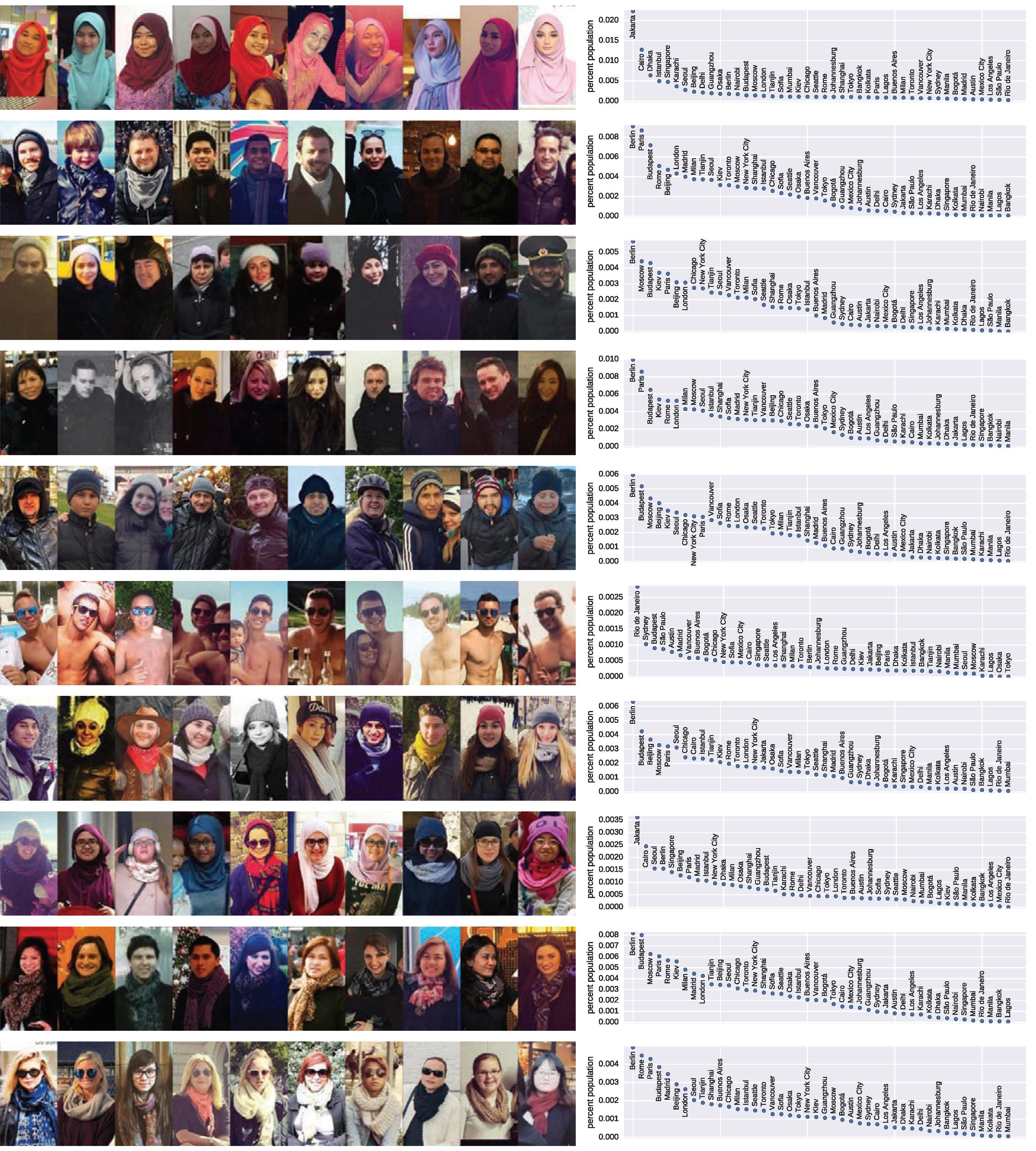
Extracting and measuring clothing style from Internet photos at scale. (a) We apply deep learning methods to learn to extract fashion attributes from images and create a visual embedding of clothing style. We use this embedding to analyze millions of Instagram photos of people sampled worldwide, in order to study spatio-temporal trends in clothing around the globe. (b) Further, using our embedding, we can cluster images to produce a global set of representative styles, from which we can (c) use temporal and geo-spatial statistics to generate concise visual depictions of what makes clothing unique in each city versus the rest.
StreetStyle: Exploring world-wide clothing styles from millions of photos
Abstract
Each day billions of photographs are uploaded to photo-sharing services and social media platforms. These images are packed with information about how people live around the world. In this paper we exploit this rich trove of data to understand fashion and style trends worldwide. We present a framework for visual discovery at scale, analyzing clothing and fashion across millions of images of people around the world and spanning several years. We introduce a large-scale dataset of photos of people annotated with clothing attributes, and use this dataset to train attribute classifiers via deep learning. We also present a method for discovering visually consistent style clusters that capture useful visual correlations in this massive dataset. Using these tools, we analyze millions of photos to derive visual insight, producing a first-of-its-kind analysis of global and per-city fashion choices and spatio-temporal trends.
keywords:
photocollections, ML, fashion, visual discovery1 Introduction
Our age of big data presents us with the compelling opportunity to use all available information to measure the world in ways that were never before possible. Large amounts of data—for instance, OCRed scans of centuries worth of books—coupled with tools for exploring this data have yielded powerful new mechanisms for scientists to study our history, culture, and behavior [\citenameMichel et al. 2010]. This opportunity is magnified by the massive scale at which humans are generating cultural artifacts on social media, and by the increasing power of machine learning techniques. For instance, by applying natural language processing to millions of Twitter messages, we can discover relationships between time of day and mood that leverage sample sizes much larger than those of any traditional study [\citenameGolder and Macy 2011].
To date, most of these new kinds of big data analyses have been limited to structured data, such as user interactions on social networks, or to textual data, such as books and tweets. However, a tremendous cache of unstructured visual information about our world is locked in images, particularly in images of people, including the billions of photos uploaded to photo-sharing services each day. Imagine a future anthropologist with access to trillions of photos of people—taken over centuries and across the world—and equipped with effective tools for analyzing these photos to derive insights. What kinds of new questions can be answered? This problem area of data-driven visual discovery is still new, but is beginning to gain attention in computer vision and graphics [\citenameDoersch et al. 2012, \citenameWang et al. 2013, \citenameZhu et al. 2014, \citenameGinosar et al. 2015, \citenameGebru et al. 2017]. Our work takes a step towards this vision by analyzing geo-spatial trends in fashion style across tens of millions of images from social media.
In this paper, we focus on clothing, as it is a critical aspect of the visual world and of our daily lives. Individuals make fashion choices based on many factors, including geography, weather, culture, and personal preference. The ability to analyze and predict trends in fashion is valuable for many applications, including analytics for fashion designers, retailers, advertisers, and manufacturers. This kind of analysis is currently done manually by analysts by, for instance, collecting and inspecting photographs from relevant locations and times.
We aim to extract meaningful insights about the geo-spatial and temporal distributions of clothing, fashion, and style around the world through social media analysis at scale. We do so through the combination of (1) millions of photos spanning the world—photos uploaded to social media services by everyday users, (2) a new dataset, StreetStyle-27k, consisting of a subset of these images annotated with fashion attributes, and (3) powerful machine learning methods based on deep learning that leverage our dataset. We explore two kinds of machine learning methods: supervised learning methods that are trained on our annotated dataset to predict clothing attributes in new images, followed by unsupervised clustering methods that can automatically detect visual correlations in our data (such as particular types of headwear, as in Figure StreetStyle: Exploring world-wide clothing styles from millions of photos(b), top row). These machine learning methods allow us to measure clothing features across millions of photos, and then to use these measurements to produce analyses in the form of trend reports and map-based visualizations, enabling new types of visual insight. For instance, our framework can help answer questions such as:
-
•
How is the frequency of scarf use in the US changing over time? (Figure 11)
- •
-
•
For a given city, such as Los Angeles, what styles are most characteristic of that city (popular in LA, but rare elsewhere)? (Figures StreetStyle: Exploring world-wide clothing styles from millions of photos(c) and 14.
Our approach also demonstrates the utility of machine learning methods for vastly simplifying the process of making real-world measurements from large-scale visual data.
In summary, our work makes the following contributions:
-
1.
StreetStyle-27k, an annotated dataset of people containing 27K images, each with 12 clothing attributes, to be made publicly available,
-
2.
a methodology for analyzing millions of photos to produce a visual clothing embedding (shown in Figure StreetStyle: Exploring world-wide clothing styles from millions of photos(a)), then using this embedding to predict clothing attributes in new photos,
-
3.
the use of unsupervised clustering methods to automatically predict visual correlations between clothing attributes (in the form of style clusters, Figure StreetStyle: Exploring world-wide clothing styles from millions of photos(b)), and
-
4.
a first-of-its-kind analysis of global and per-city fashion choices and trends using our machine learning methods.
We provide additional visualizations of our results at http://streetstyle.cs.cornell.edu.
2 Related Work
Visual discovery. Researchers are beginning to mine world-wide imagery to (1) discover visual trends and (2) measure aspects of the world over space and time. Much of this work has looked at places. Doersch et al. pioneered the idea of computational geography and explored the distinctive visual characteristics of cities through Street View imagery \shortcitedoersch:siggraph:2012, driven by weakly supervised methods for finding discriminative elements [\citenameSingh et al. 2012, \citenameDoersch et al. 2013]. Such visual characteristics can also be correlated to other properties of cities, such as perceived safety [\citenameArietta et al. 2014, \citenameNaik et al. 2014, \citenameDubey et al. 2016]. These correlations can then be used to automatically predict such properties across a city simply from ground level images. Beyond analyses of cities, computer vision techniques have been used to answer questions such as “is there snow in this photo?” or “are there clouds in this webcam?” which in turn can be used at scale to estimate maps of snow or cloud cover over large regions of the world [\citenameZhang et al. 2012, \citenameMurdock et al. 2015].
Other work has used large image collections to study people, including explorations of how people move through cities [\citenameCrandall et al. 2009], the relationship between facial appearance and geolocation/time [\citenameIslam et al. 2015, \citenameSalem et al. 2016], analysis of expressions and styles over a century in high school yearbook photos [\citenameGinosar et al. 2015], and tools for discovering visual patterns that distinguish two populations [\citenameMatzen and Snavely 2015]. Finally, Gebru et al. study demographics across the US by detecting and analyzing cars (along with their makes and models) in Street View imagery \shortcitegebru:arxiv:2017. Compared to this prior work, we focus on a different domain, fashion and style, and apply our work to a much broader sample of people by using worldwide images on social media.
Visual understanding of clothing. Clothing is a rich, complex visual domain from the standpoint of computer vision, because clothing analysis combines a detailed attribute-level understanding with social context. We build on previous work that describes people in terms of clothing and other fashion attributes, such as “wearing glasses,” or “short sleeves,” and recognizes these attributes in new images [\citenameChen et al. 2012, \citenameBourdev et al. 2011, \citenameBossard et al. 2013, \citenameZhang et al. 2014]. Beyond classifying attributes, other work also produces full pixel-level clothing segmentations [\citenameYamaguchi et al. 2012, \citenameYamaguchi et al. 2013, \citenameYang et al. 2014], or recognizes specific (or similar) products rather than general attributes [\citenameDi et al. 2013, \citenameVittayakorn et al. 2015, \citenameKiapour et al. 2015]. Other work categorizes clothing in terms of explicit, named styles. For instance, Kiapor et al. used a game to analyze coarse fashion styles such as “hipster” and “goth” to build inter-style classifiers (i.e., is this photo goth or hipster?) and intra-style ranking functions (i.e., how hipster is this person’s fashion?) \shortcitekiapour:eccv:2014. In our work, we train classifiers using coarse-grained attributes, but then leverage this training to organize images visually in order to perform more fine-grained clustering.
Clothing trends. Spatial and temporal fashion trends have been explored in computer vision, but usally on small samples sizes and with limited statistical analysis. Hidayati et al. analyze catwalk images from NYC fashion shows to find style trends in high-end fashion \shortcitehidayati:acmmm:2014. Simo-Serra et al. analyzed chictopia.com to study correlations between fashionability and other attributes such as wealth, as well as temporal trends (e.g., a sudden spike in popularity of heels in Manila) \shortcitesimoserra:cvpr:2015. [\citenameVittayakorn et al. 2015] showed that seasonal trends related to styles such as “floral”, “pastel”, and “neon” can be found using fashion classifiers, with the peak occurring in the springtime. [\citenameHe and McAuley 2016] modeled per-user fashion taste over time and found certain styles had a resurgence in the late 2000s. However, these trends were not evaluated for statistical significance, and so it is challenging to conclusively distinguish signal from noise. We argue that without the massive amounts of data we advocate, it is difficult to establish such significance.
Clothing datasets. Most previous clothing style datasets have been very limited in scale, and biased towards images of the fashion-conscious. For example, several efforts have made use of fashion-centric social networking sites such as fashionista.com and chictopia.com [\citenameYang et al. 2014, \citenameSimo-Serra et al. 2015, \citenameYamaguchi et al. 2015, \citenameYamaguchi et al. 2012, \citenameYamaguchi et al. 2013]. These sites enable users to upload photos and annotate articles of clothing for the express purpose of modeling their style. Other work draws on online clothing retailers such as Amazon, eBay, and ModShop to build similar datasets [\citenameLiu et al. 2012, \citenameDi et al. 2013, \citenameKiapour et al. 2015]. Images from these websites are relatively clean and organized according to tags, facilitating the creation of annotated datasets on the scale of hundreds of thousands of people [\citenameChen et al. 2012, \citenameBossard et al. 2013]. However, our goal is to measure spatio-temporal trends over the entire world from real-world images, and to obtain highly certain statistics, so very large data is key—100K images is insufficient, once the data is sliced in time and space. Furthermore, fashion sites are designed to engage the fashion-conscious, whereas our goal is to analyze the world’s populace at large. Our approach is to build a massive dataset from photos on social media, which can be gathered at larger scale and are more representative of everyday fashions (hence the name StreetStyle). However, these images are also much more noisy and are often not tagged according to clothing. Therefore, we annotate a small subset of our large dataset manually, and use machine learning to generalize the result to the rest of the dataset.
3 Data
Out dataset consists of three key parts: (1) photos, (2) the people in those photos, and (3) the clothing attributes of those people.
Photos. The photos we use in our analysis were acquired via Instagram, a popular mobile photography social network. We chose Instagram due to the sheer volume of uploads—an advertised 95 million photos/videos per day111http://time.com/4375747/instagram-500-million-users/—as well as their providing a public photo search API.222https://www.instagram.com/developer/ Users can query this API to retrieve images that have been uploaded within a 5 kilometer radius of a specified latitude and longitude and within 5 days of a specified date.
| Austin | Bangkok | Beijing | Berlin |
| Bogotá | Budapest | Buenos Aires | Cairo |
| Chicago | Delhi | Dhaka | Guangzhou |
| Istanbul | Jakarta | Johannesburg | Karachi |
| Kiev | Kolkata | Lagos | London |
| Los Angeles | Madrid | Manila | Mexico City |
| Milan | Moscow | Mumbai | Nairobi |
| New York City | Osaka | Paris | Rio de Janeiro |
| Rome | São Paulo | Seattle | Seoul |
| Shanghai | Singapore | Sofia | Sydney |
| Tianjin | Tokyo | Toronto | Vancouver |
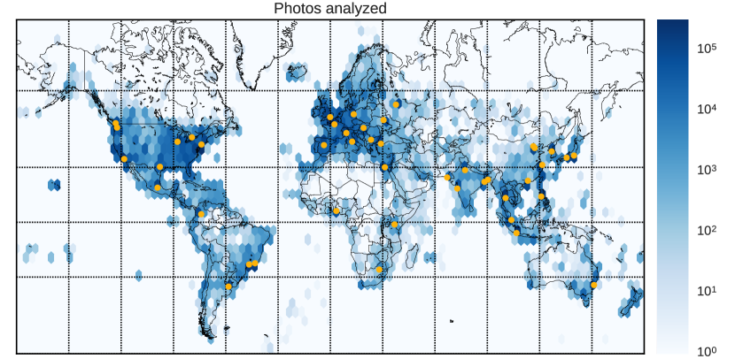
How should we sample photos geographically? To answer this question, we consider two types of experiments we wish to conduct: (1) a comparison of major world population centers, and (2) a nation-, continent-, or world-wide analysis of styles and trends. To sample photos for goal (1) (analysis of urban centers), we made a list of 44 major cities spanning six continents, each with a lat/long approximating the city center, shown as yellow dots in Figure 1. The complete list of cities is shown in Table 1. For each city, we sampled photos centered on those coordinates from Instagram. To sample photos for goal (2) (globally distributed photos), we used the Flickr 100M photo dataset [\citenameThomee et al. 2015] to derive a distribution of photo uploads over the globe. In particular, we extracted the approximately 48 million geotags from Flickr 100M, and used these geotags to compute a geographic distribution from which to sample photos from Instagram. This distribution (after filtering by person detection, as discussed below) is shown in blue in Figure 1.
For both sampling strategies, we uniformly sampled a 5-day window from June 2013—the earliest date Instagram provided results—until June 2016. For each photo, we record its geolocation and timestamp. In total, we retrieved over 100 million photos.
People. To find people in photos, we ran two out-of-the-box vision algorithms on each downloaded photo, one to detect and localize faces, and the second to estimate the visibility of the rest of the body. To detect faces, we used the API provided by Face++.333http://www.faceplusplus.com/ The output of the Face++ detector is a bounding box for the face, as well as facial landmark keypoints. We use the face bounding box to geometrically align people in our analysis algorithms. To determine body visibility, we use the Deformable Part Model [\citenameFelzenszwalb et al. 2010, \citenameGirshick et al. 2012] and the provided person detector trained on VOC2010 [\citenameEveringham et al. 2010].
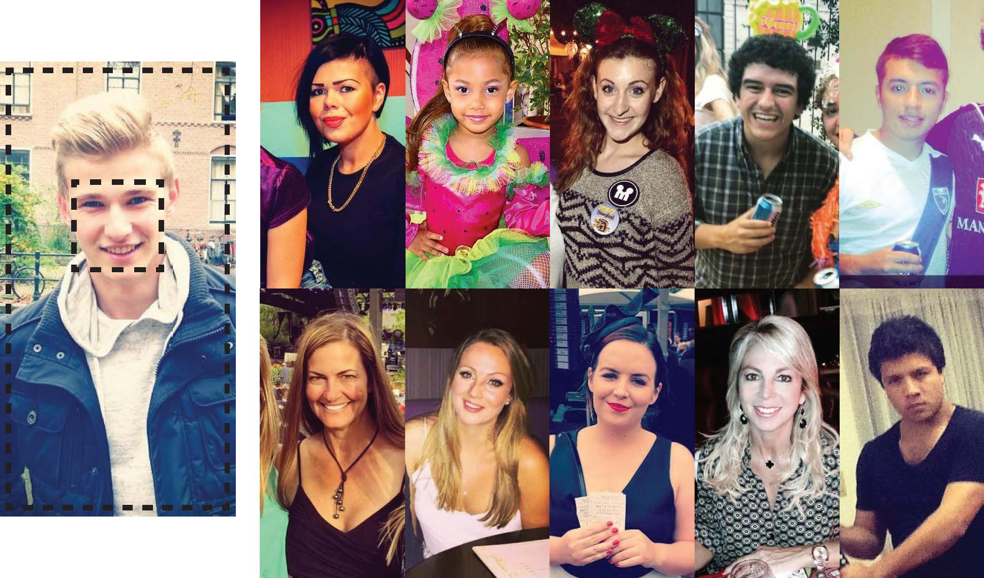
Given a set of faces and visible bodies in a photo, we pair them up using a simple distance-based heuristic. For each face, we compute a canonical image crop based on the position and scale of the detected face, illustrated in Figure 2. If the crop extends beyond the visible body bounding box, we discard the detection.
In total, out of the more than 100 million photos we retrieved from Instagram, 37.7 million had at least one successful person detection. For our work, we chose to keep detections with at least the face and torso visible. We do not analyze the lower part of the body since the legs are often occluded in online photos. After generating canonical crops from the face detections and filtering on face and torso visibility, we gathered a total of 14.5 million images of people.
| No | Yes | |
|---|---|---|
| Wearing Jacket | 18078 | 7113 |
| Collar Presence | 16774 | 7299 |
| Wearing Scarf | 23979 | 1452 |
| Wearing Necktie | 24843 | 827 |
| Wearing Hat | 23279 | 2255 |
| Wearing Glasses | 22058 | 3401 |
| Multiple Layers | 15921 | 8829 |
| Major |
| Color |
| Black (6545) |
| White (4461) |
| 2+ colors (2439) |
| Blue (2419) |
| Gray (1345) |
| Red (1131) |
| Pink (649) |
| Green (526) |
| Yellow (441) |
| Brown (386) |
| Purple (170) |
| Orange (162) |
| Cyan (33) |
| Clothing |
| Category |
| Shirt (4666) |
| Outerwear (4580) |
| T-shirt (4580) |
| Dress (2558) |
| Tank top (1348) |
| Suit (1143) |
| Sweater (874) |
| Sleeve |
| Length |
| Long sleeve (13410) |
| Short sleeve (7145) |
| No sleeve (3520) |
| Neckline |
| Shape |
| Round (9799) |
| Folded (8119) |
| V-shape (2017) |
| Clothing |
| Pattern |
| Solid (15933) |
| Graphics (3832) |
| Striped (1069) |
| Floral (885) |
| Plaid (532) |
| Spotted (241) |
Clothing annotations. For each person in our corpus of images, we want to extract fashion information. To do so, we first collect annotations related to fashion and style for a subset of the data, which we later use to learn attribute classifiers that can be applied to the entire corpus. Example attributes include: What kind of pattern appears on this shirt? What is the neckline? What is the pattern? Is this person wearing a hat? We created a list of several clothing attributes we wished to study a priori, such as clothing type, pattern, and color. We also surveyed prior work on clothing attribute recognition and created a consolidated list of attributes that we observed to be frequent and identifiable in our imagery. We began with several of the attributes presented by Chen et al. [\citenameChen et al. 2012] and made a few adjustments to more clearly articulate neckline type as in the work of Di et al. [\citenameDi et al. 2013]. Finally, we added a few attributes of our own, including wearing-hat and wearing-jacket, as well as an attribute indicating whether or not more than one layer of clothing is visible (e.g., a suit jacket over a shirt or an open jacket showing a t-shirt underneath). Table 2 shows our full list of attributes.
We annotated a 27K-person subset of our person image corpus with these attributes using Amazon Mechanical Turk. Each Mechanical Turk user was given a list of 40 photos, presented one-by-one, and asked to select one of several predefined attribute labels. In addition, the user could indicate that the person detection was faulty in one of several ways, such as containing more than one person or containing no person at all. Each set of 40 photos contained two photos with known ground truth label as sentinels. If a worker failed at least five sentinels and their sentinel failure rate was above 20%, we prevented them from performing any more work for our tasks. Compensation for a single attribute on a set of 40 photos was 0.10 USD. Average wage was approximately 4 USD / hour. An attribute for an image was labeled by five separate workers, and a different set of five workers labeled each attribute for an image. A label was accepted if 3 / 5 workers agreed, otherwise it was excluded from the data. In total these annotations cost approximately 4K USD. We refer to our annotated dataset as StreetStyle-27k.
Dataset bias and limitations. Any dataset has inherent bias, and it is important to be cognizant of these biases when drawing conclusions from the data. Instagram is a mobile social network, so participants are more likely to be in regions where broadband mobile Internet is available, and where access to Instagram is not censored or blocked. In some areas, people might be more likely to upload to a competitor service than to Instagram. People of certain ages might be more or less likely to upload to any social network. Cultural norms can affect who, when, where, and what people photograph. The face detector we use is an off-the-shelf component for which no reported statistics regarding bias for age, gender, and race are made available. The person detector has also not been evaluated to determine bias in these factors either. These factors impact who will and will not be properly added to our dataset, which could introduce bias. As vision methods mature, analyses for such bias will become increasingly important.
4 Machine Learning Methodology
To make measurements across the millions of photos in our dataset, we wish to generalize labeled data from StreetStyle-27k to the entire corpus. For instance, to measure instances of glasses across the world, we want to use all of the wearing-glasses annotations as training data and predict the wearing-glasses attribute in millions of unlabeled images. To do so we use Convolutional Neural Networks (CNNs) [\citenameKrizhevsky et al. 2012]. A CNN maps an input (e.g., the pixels of an image), to an output (e.g., a binary label representing whether or not the person is wearing glasses), by automatically learning a rich hierarchy of internal image features given training data. In this section, we describe the architecture of our particular CNN, how we trained it using our labeled attribute dataset, and how we evaluated the classifier’s performance on the clothing attribute prediction task. We then discuss how and when it is appropriate to generate predictions from this CNN across millions of photos and use these predictions to estimate real-world fashion statistics.
4.1 Learning attributes
A key design decision in creating a CNN is defining its network architecture, or how the various types of internal image processing layers are composed. The penultimate layer of a typical CNN outputs a multi-dimensional (e.g., 1024-D) feature vector, which is followed by a “linear layer” (matrix product) operation that outputs one or more prediction scores (e.g., values indicating the probability of a set of attributes of interest, such as wearing-glasses). The base architecture for our CNN is the “GoogLeNet” architecture [\citenameSzegedy et al. 2015]. While several excellent alternatives exist (such as VGG [\citenameSimonyan and Zisserman 2014]), GoogLeNet offers a good tradeoff between accuracy on tasks such as image classification [\citenameRussakovsky et al. 2015] and speed. As with other moderate-sized datasets (fewer than 1 million training examples), it is difficult to train a CNN on our attribute prediction task from scratch without overfitting. Instead, we start with a CNN pretrained on image classification (on ImageNet ILSVRC2012) and fine-tune the CNN on our data. After ImageNet training, we discard the last linear layer of the network to expose the 1024-dimensional feature output and then append several linear layers in parallel where is the number of class labels for attribute (for instance, for a binary attribute such as wearing-glasses, and for neckline shape as we consider three possible shapes).
Training details. We train the CNN as follows. For each attribute, we use stratified sampling to first select an attribute label and then a particular example image with that label. This sampling strategy counteracts the implicit imbalance within each attribute (e.g., wearing a hat is much less common than not wearing a hat). We do this 32 times to build a single mini-batch of images. Using this mini-batch, we apply the forward and backward passes of the CNN to compute the parameter gradient with respect to the cross-entropy loss. We do this for each attribute, accumulating the gradients. Then we use stochastic gradient descent with momentum , learning rate , and weight decay to update the parameters of the CNN. We fine-tune the CNN for 6,000 iterations ( attributes) after which the mean class accuracy on a validation set stopped increasing. 80% of StreetStyle-27k was used for training, 10% was used as validation to determine when to stop training as well as for the additional analysis in this section, and 10% was used as a test set for a final evaluation of the attribute classification task.
| Attribute |
|
Random guessing | Majority guessing | ||
|---|---|---|---|---|---|
| wearing jacket | 0.869 / 0.848 | 0.5 / 0.5 | 0.698 / 0.5 | ||
| clothing category | 0.661 / 0.627 | 0.142 / 0.142 | 0.241 / 0.142 | ||
| sleeve length | 0.794 / 0.788 | 0.333 / 0.333 | 0.573 / 0.333 | ||
| neckline shape | 0.831 / 0.766 | 0.333 / 0.333 | 0.481 / 0.333 | ||
| collar presence | 0.869 / 0.868 | 0.5 / 0.5 | 0.701 / 0.5 | ||
| wearing scarf | 0.944 / 0.772 | 0.5 / 0.5 | 0.926 / 0.5 | ||
| wearing necktie | 0.979 / 0.826 | 0.5 / 0.5 | 0.956 / 0.5 | ||
| clothing pattern | 0.853 / 0.772 | 0.166 / 0.166 | 0.717 / 0.166 | ||
| major color | 0.688 / 0.568 | 0.077 / 0.077 | 0.197 / 0.077 | ||
| wearing hat | 0.959 / 0.917 | 0.5 / 0.5 | 0.904 / 0.5 | ||
| wearing glasses | 0.982 / 0.945 | 0.5 / 0.5 | 0.863 / 0.5 | ||
| multiple layers | 0.830 / 0.823 | 0.5 / 0.5 | 0.619 / 0.5 |
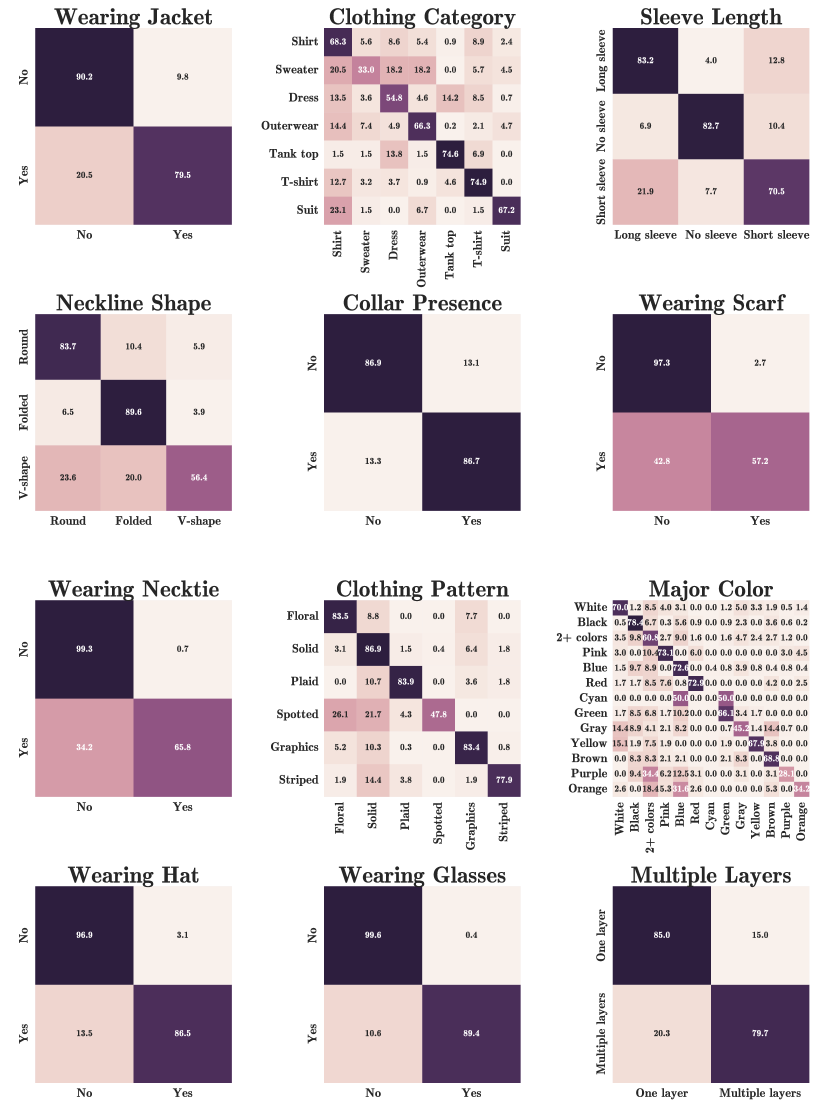
Table 3 summarizes the accuracy and mean class accuracy of our learned classifiers for each attribute on the held-out test set. Figure 3 shows a set of confusion matrices, one per attribute, illustrating which attributes tend to get confused for one another (e.g., spotted shirts can be mistaken for floral shirts). While the classifiers perform quite well in general (e.g., wearing-hat has an accuracy over 90%), even state-of-the-art CNNs make mistakes, and so all of the classifiers have an inherent error level. We now discuss how we take this error into account when using these classifiers.
4.2 Measuring attributes at scale
Our aim is not just to build a classifier for each clothing attribute and maximize some performance criterion on a test set, but to take that learned classifier, apply it to a much larger corpus of images spanning years worth of the world’s photos, and provide a tool for discovering interesting trends. However, the classifiers are not perfect, and any real-world measurement is going to have some noise. While it is inevitable that a classifier will have some non-zero variance, the hope is that the estimation is unbiased, that is, as we increase the sample size, a computed statistic, such as the detected percentage of people wearing hats in photos, will converge on the true percentage of people wearing hats. However, by examining the confusion matrices in Figure 3 it becomes clear that this will not be the case. For example, the proportion of images featuring people wearing neckties is much less than 50%. For this attribute, the classifier predicts No correctly 99% of the time, but Yes correctly only 65% of the time. Therefore, the estimate of the percentage of people wearing neckties in photos will be biased towards No.
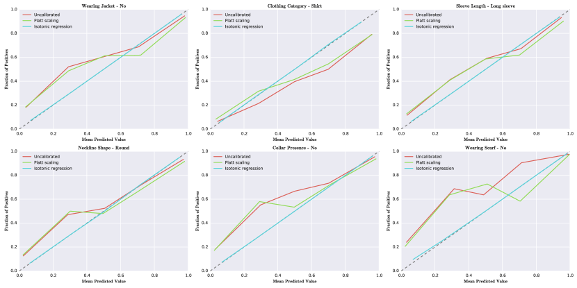
One way to mitigate this bias is to calibrate the scores of a classifier using a function that models the posterior probability of the classification being correct given the classification score. There are several methods for this type of calibration, including Platt scaling (an application of logistic regression) [\citenamePlatt 1999] and isotonic regression. Others have noted that neural networks tend not to require calibration as severely as classifiers such as SVMs and boosted decision trees [\citenameNiculescu-Mizil and Caruana 2005]. Nevertheless, we found that our networks benefited from calibration by applying isotonic regression to our validation set. Figure 4 shows the generalization performance of calibration for several attribute labels. Note that after isotonic regression, the curves are very close to the identify function (), which means that these curves are properly calibrated. In our experiments, half of the validation set was used for training the regressor and the other half was used to generate reliability curves. Isotonic regression typically requires more data to avoid overfitting, yet is more flexible when the calibration required is not sigmoidal, an underlying assumption of Platt scaling. The generalization shows that these estimates do not exhibit severe overfitting and therefore we opt to use isotonic regression trained on the entire validation set to calibrate the scores.
4.3 Visually consistent style clusters
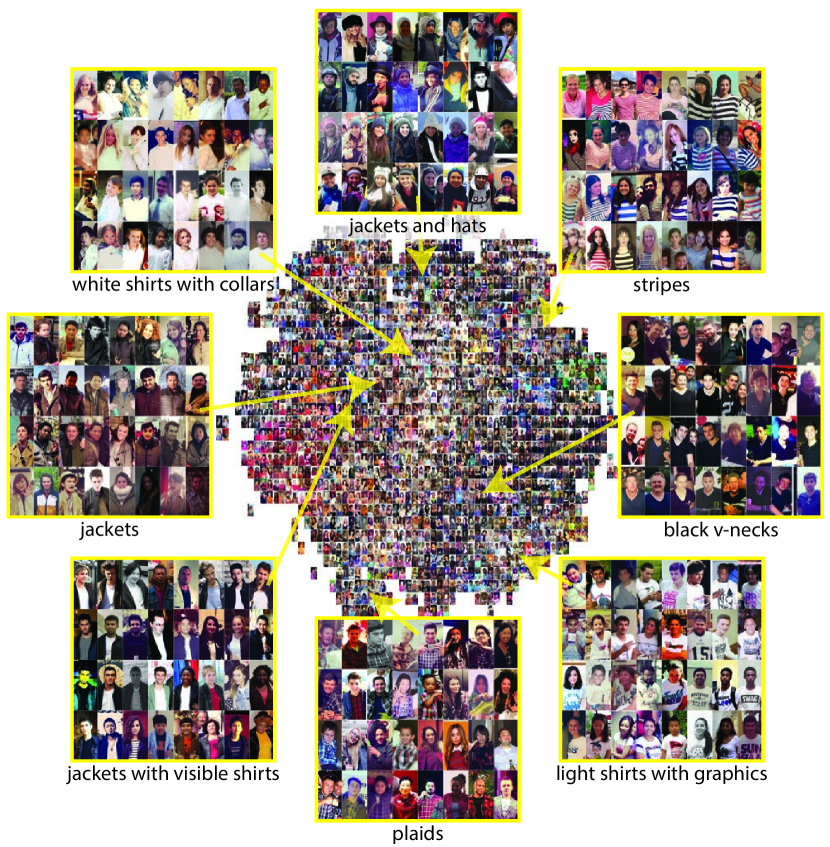

The predicted attributes are immediately useful in plotting and analyzing trends, such as “how is the proportion of people wearing black in Los Angeles changing over time?” as we demonstrate in Section 5. However, we would like to analyze clothing styles beyond these attributes in a number of ways:
-
•
Identify common, visually correlated combinations of these basic attributes (e.g., blue sweater with jacket and wool hat).
-
•
Identify styles that appear more frequently in one city versus another or more frequently during particular periods of time.
-
•
Identify finer-grained, visually coherent versions of these elements (e.g., sports jerseys in a particular style).
To achieve these goals, we use clustering to identify recurring visual themes in the embedded space of people. Recall that the penultimate layer of our network is a 1024-dimensional feature space where distinct fashion attributes are linearly separable. Figure 5 shows a visualization of this feature space projected to 2D using t-SNE [\citenamevan der Maaten and Hinton 2008]. Within this 1024-D feature space, people images are organized according to visual fashion attributes, through the mechanism of training on our StreetStyle-27k dataset. The ideas is that by clustering images in this 1024-D embedded feature space, we can discover and reveal visual themes such as those described above. We refer to such clusters as style clusters. Once we identify style clusters, we can further characterize cities and times in terms of these clusters—for instance, we might discover that some clusters are heavily correlated with one or two particular cities, as we explore in Section 5. Figure 6 shows an example of several style clusters found by our approach.
To find style clusters, we ran a clustering algorithm on a subset of the full dataset, for efficiency and to achieve balance between different times and regions of the world. In particular, we divided our images into bins by city and by week (e.g., Paris in week 26 of 2015). For bins with fewer than images, we selected all images, and for bins with more than images, we randomly selected images. For our experiments, we set , for a total of 5.4M sample images for clustering in total.
For each cropped person image in this set, we compute its 1024-D CNN feature vector and normalize this vector. We run PCA on these normalized vectors, and project onto the top principal components that retain 90% of the variance in the vectors (in our case, 165 dimensions). To cluster these vectors, we used a Gaussian mixture model (GMM) of 400 components with diagonal covariance matrices. Each person is assigned to the mixture component (style cluster) which maximizes the posterior probability. The people assigned to a cluster are then sorted by their Euclidean distance from the cluster center, as depicted in Figure 6. Although more clusters would increase the likelihood of the data under the model, it would also lead to smaller clusters, and so we selected 400 as a compromise between retaining large clusters and maximizing the likelihood of the data.
The resulting 400 style clusters have sizes ranging from 1K to 115K. Each style cluster tends to represent some combination of our chosen attributes, and together form a global visual vocabulary for fashion. We assign further meaning to these clusters by ranking them and ranking the people within each cluster, as we demonstrate in Section 5.2, with many such ranked clusters shown in Figures 14 and 15.
5 Exploratory Analysis
A key goal of our work is to take automatic predictions from machine learning and derive statistics from which we can find trends. Some of these may be commonsense trends that validate the approach, while others may be unexpected. This section describes several ways to explore our fashion data, and presents insights one can derive through this exploratory data analysis.
5.1 Analyzing trends
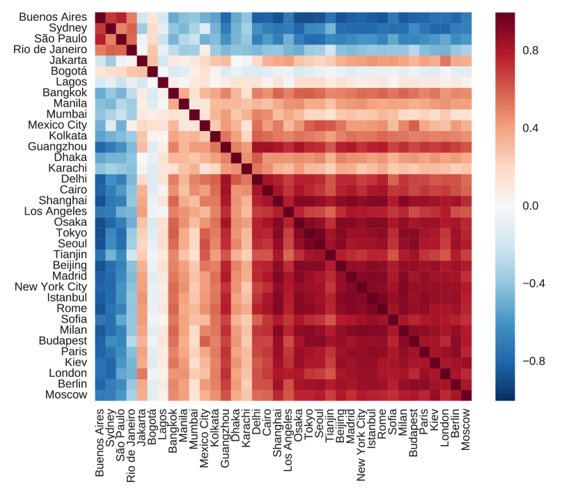
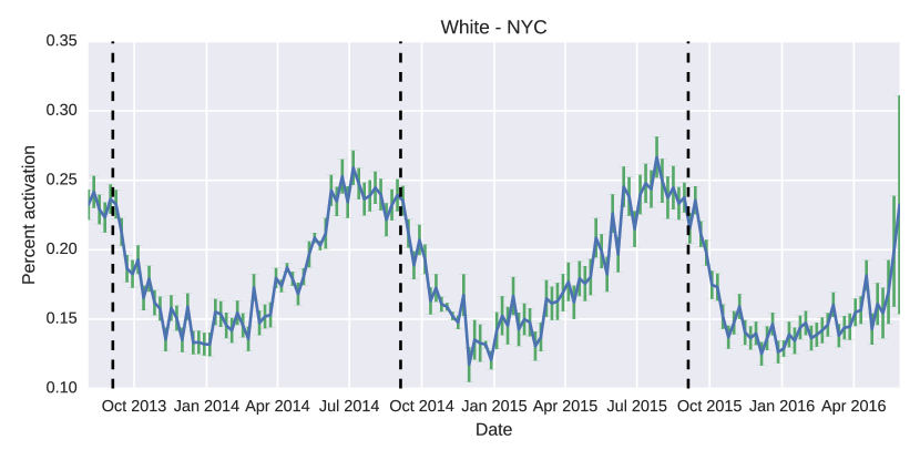
Color. How does color vary over time? Figure 7 shows plots of the frequency of appearance (across the entire world) of several colors over time. White and black clothing, for example, exhibit a highly periodic trend; white is at its maximum ( frequency) in September, whereas black is nearly reversed, much more common in January. However, if we break down these plots per city, we find that cities in the Southern Hemisphere flip this pattern, suggesting a correlation between season and clothing color. Figure 8 shows such plots for two cities, along with a visualization of all pairs of cities correlated by their white color temporal profiles, with cities reordered by latitude to highlight this seasonal effect. Cities in the same hemisphere tend to be highly correlated with one another, while cities in opposite hemispheres are highly negatively correlated. In the United States, there is an oft-cited rule that one should not wear white after the Labor Day holiday (early September). Does this rule comport with actual observed behavior? Using our method, we can extract meaningful data that supports the claim that there is a significant decrease in white clothing that begins mid-September, shortly after Labor Day, shown in Figure 9.
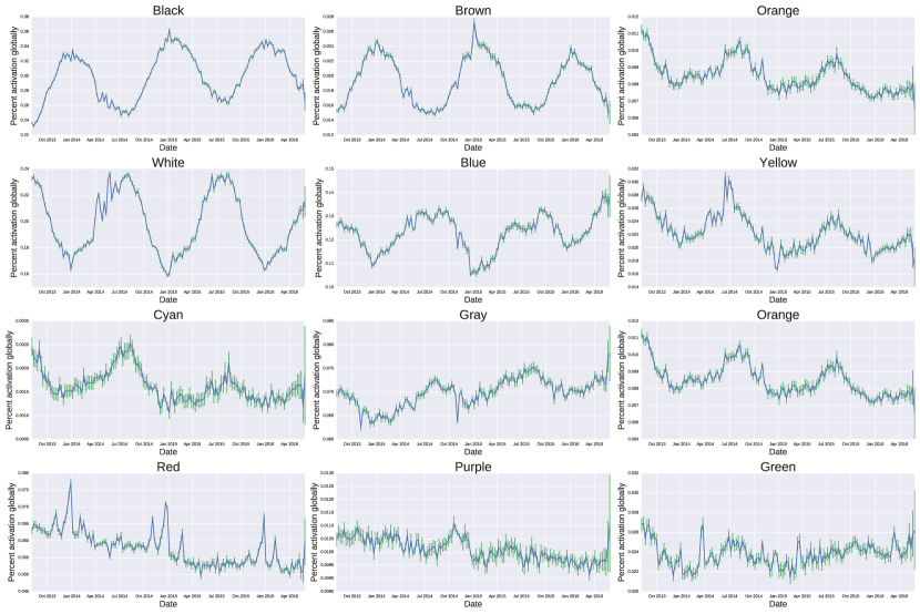

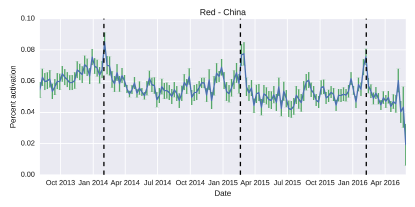
Other colors exhibit interesting, but more subtle trends. The color red is much less periodic, and appears to have been experiencing a downward trend, down approximately 1% since a few years ago. There are also several spikes in frequency that appear each year, including one small spike near the end of each October and a much larger spike near the end of each December—that is, near Halloween and Christmas. We examined our style clusters and found one that contained images with red clothing and had spikes at the same two times of the year. This cluster was not just red, but red hats. An assortment of winter knit beanies and red jacket hoods were present, but what stood out were a large assortment of Santa hats as well as an unexpected assortment of red Halloween costumes with red hats or hoods. It appears that red hats are uncommon enough that when they do appear they are highly correlated with the exceptional sorts of costumes worn on these two holidays. Finally, the Chinese New Year sees a similar spike in the color red in 2015 and 2016, as shown in Figure 10 (frequency of red clothing in China).
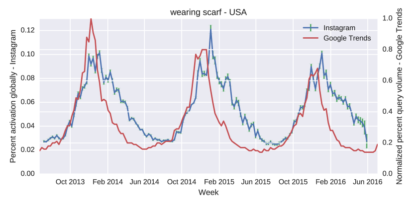
Clothing types. We can also explore more functional clothing attributes. For example, we know people wear scarves in cold weather, so one would expect to see a seasonal trend in this attribute. Figure 11 shows such a trend for visual occurrence of scarves in the United States. Moreover, we can also compare with a secondary source of information to estimate this signal, Google Trends.444https://www.google.com/trends/explore#q=scarf&geo=US Google Trends provides historical trend data for Google Search queries. By comparing these two signals, we can make several observations. First, the shapes of the signals are similar. Both feature a sudden attack and decay rather than a purely sinusoidal shape. This correlation increases our confidence that our vision-based signal is measuring something reasonable. Second, the onset of the signal derived from Google Trends tends to come prior to the onset from the Instagram photos. One explanation for this behavior is that people are searching for scarves on Google in order to purchase them and Instagram allows us to measure when they are actually wearing them. Third, while Google Trends suggests that scarves are in a significant downward annual trend, the Instagram results serve to constrast this trend (scarves are up in the winter of 2014-2015). While more study would be needed to determine the cause of such a phenomenon, this comparison illustrates the utility of our approach for devising new hypotheses for follow-up investigation. The visual data and the Google search data combine to give us a richer sense of what is happening in the world, and allow us to formulate new views about the underlying human behavior.
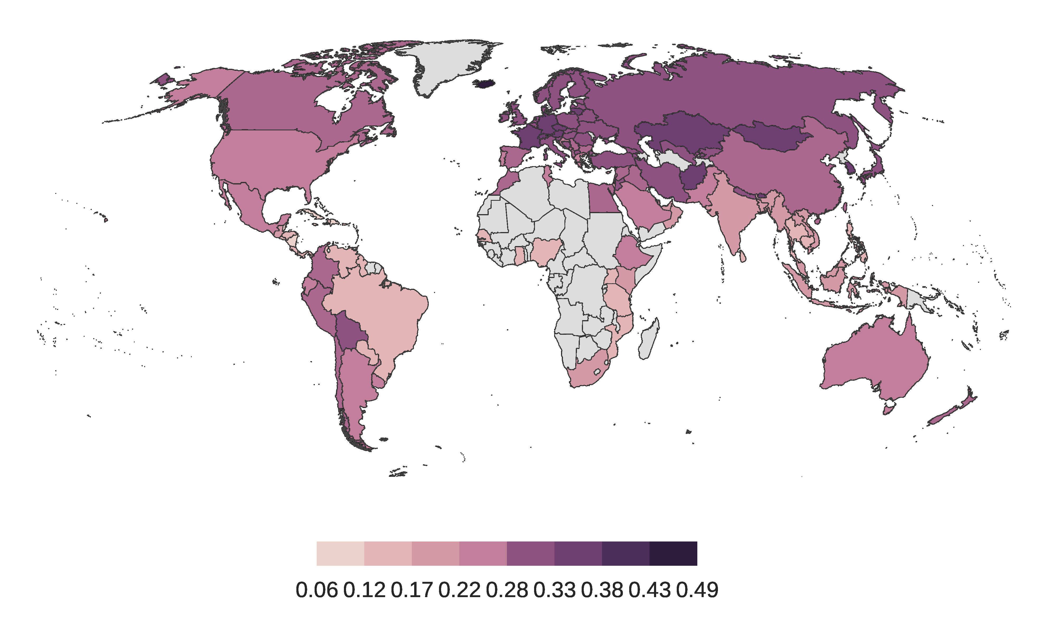

So far we have focused on temporal trends, but we can also explore geographic trends. Can we validate our attribute classifications using prior knowledge of climate and weather-related clothing? For example, where in the world do people wear jackets? Figure 12 shows the percentage of detected people who are wearing jackets, broken down by country. This map accords with intuition. Countries further north tend to feature more jackets. In South America, more jackets are found as you go further west (e.g., in Boliva or Colombia)—winter clothes will tend to be worn more often at higher elevation (in this case in the Andes) than at lower elevations.
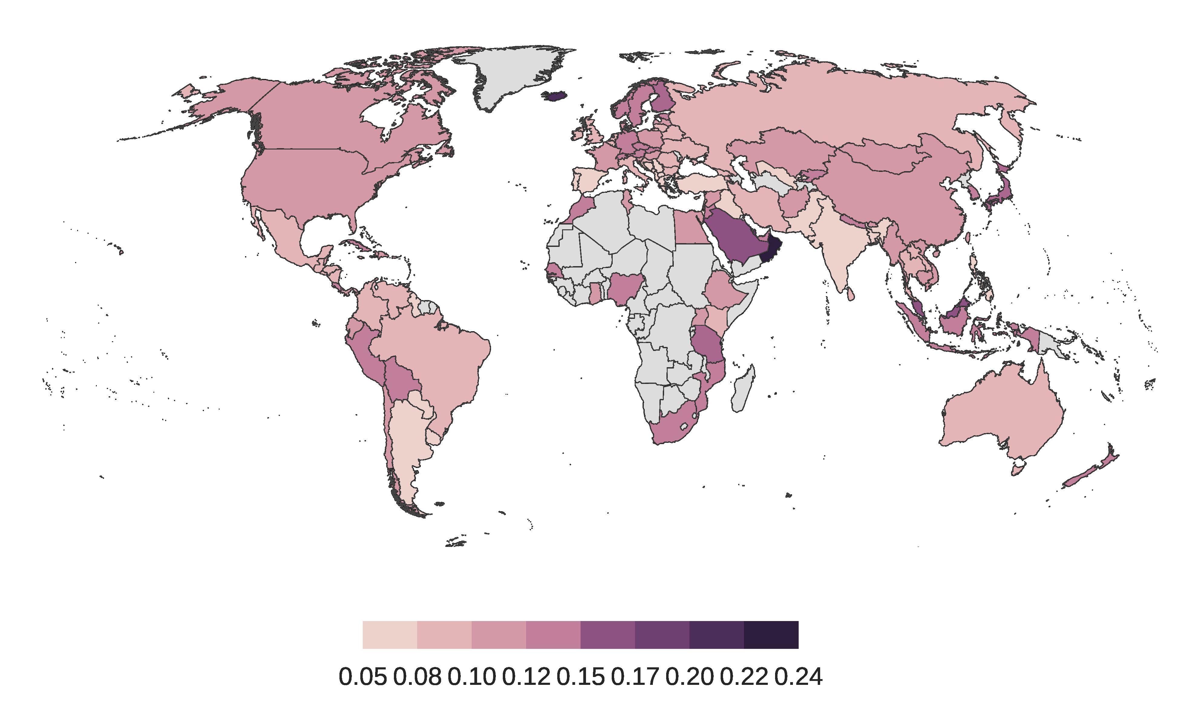
What about more unexpected geographic trends? Where in the world are people wearing hats? Figure 13 shows the percentage of photos per country that contain people wearing hats. Once again, people wear hats in colder places, but interestingly in Oman, hats are evidently extremely popular. Figure 13 shows several examples of images from Oman that are highly ranked as wearing hats. In particular, the kuma and massar are popular in Oman, as they are an important element of the men’s national dress.
5.2 Visualizing styles
We also wish to visualize commonly occuring combinations of attributes, or “styles.” To visualize styles, we use the method in Section 4.3 to compute style clusters from the embedded photos. Figure 6 shows several such clusters, in no particular order. Given these clusters, then for every photo in our dataset, we compute the style cluster centroid to which it is closest. We can then perform additional analyses using these style clusters, such as plotting the frequency of visual occurrence of each cluster across space and time to mine for styles that are well localized in one or both.
 |
| Top five clusters sorted by space-time entropy. |
 |
| Bottom five clusters sorted by space-time entropy. |
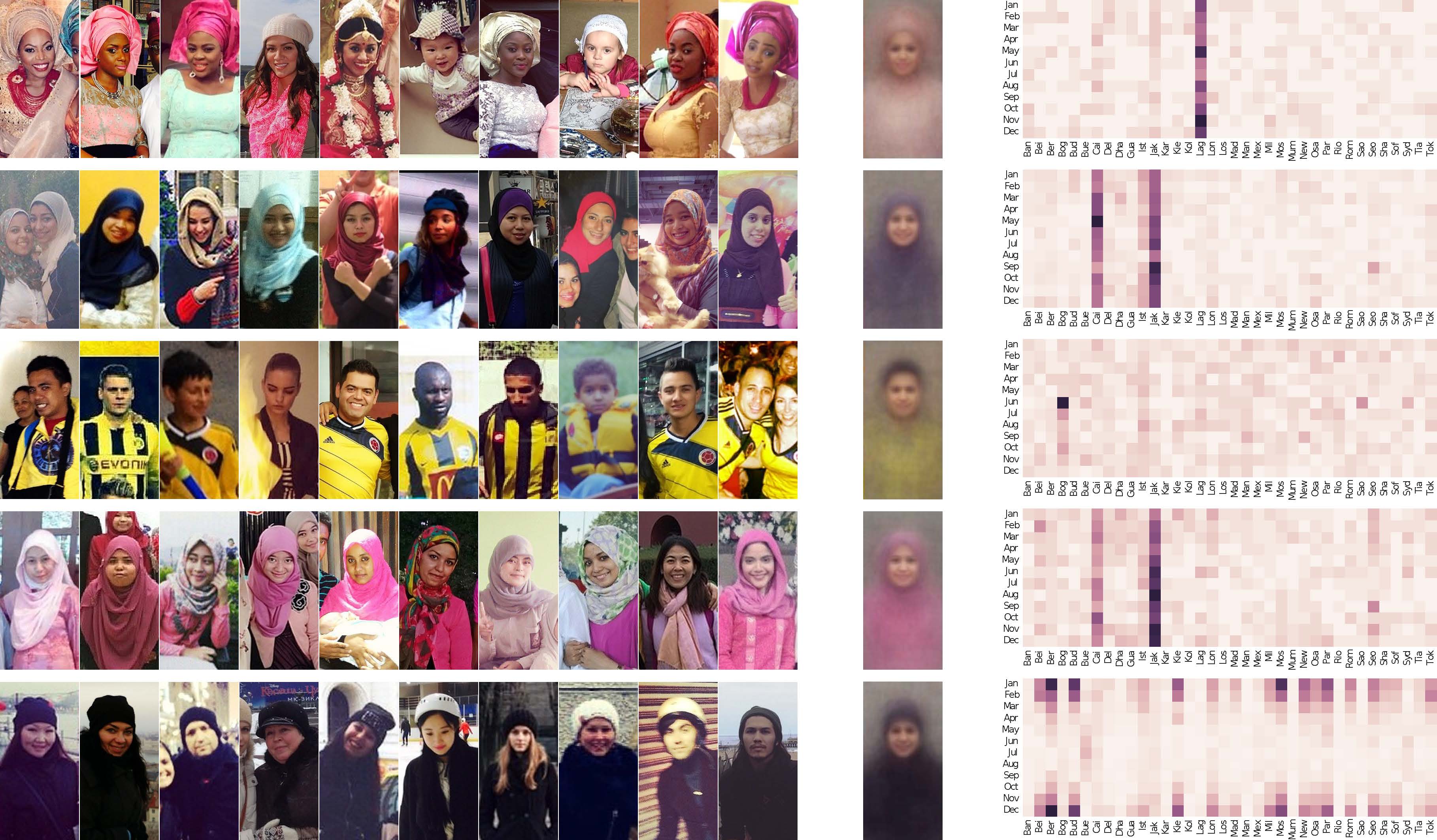
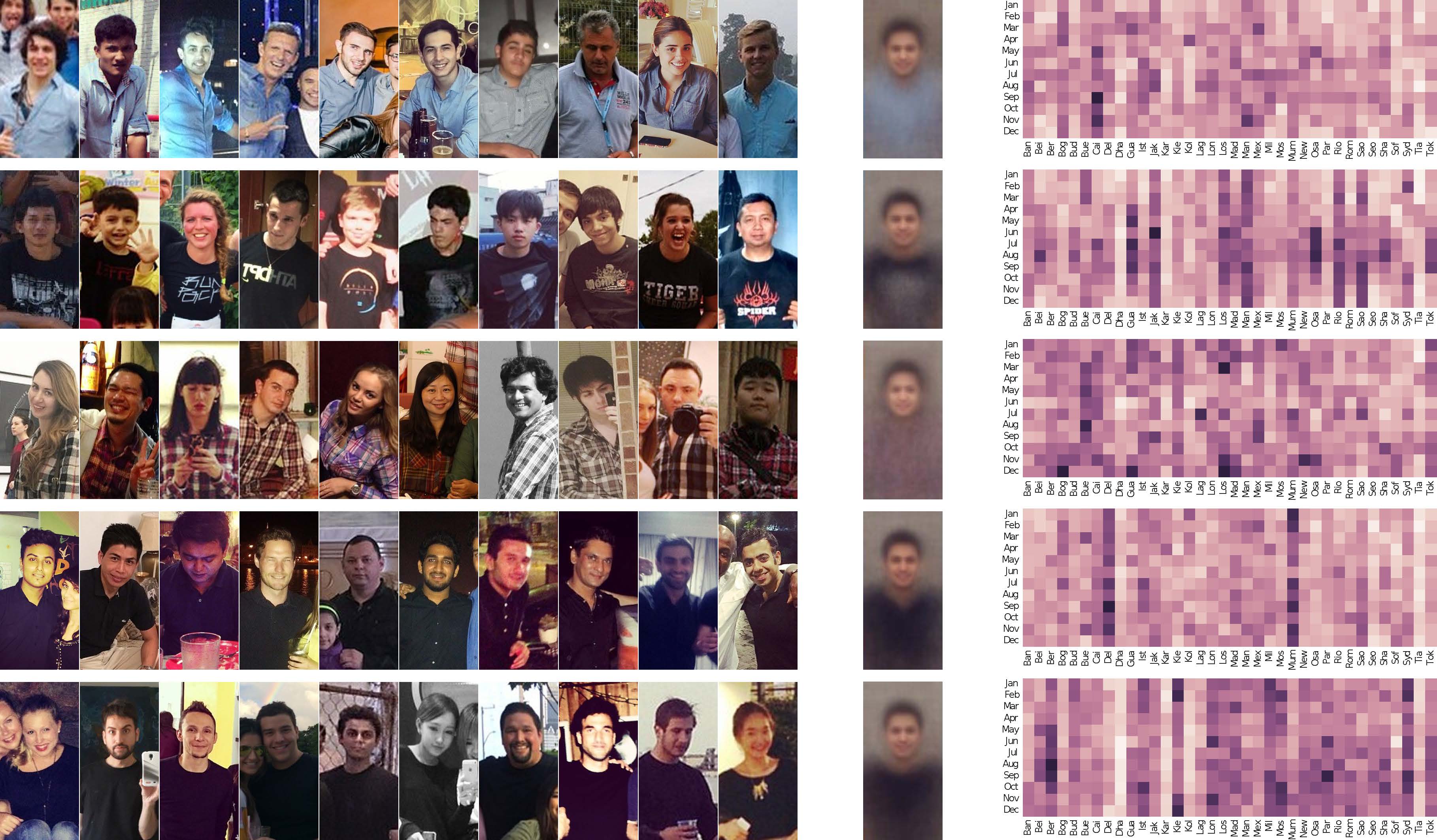
This raw visualization of style clusters is not particularly easy to explore, as there are hundreds of such clusters. Therefore, it is useful to define a ranking function to help surface the most interesting signals. One way to rank clusters is according to entropy over the different cities in the dataset—high-entropy clusters will tend to be specific to a few cities, while low-entropy clusters tend to be universal. Figure 14 shows the top clusters for such a ranking. This ranking helps provide a sense of how geography affects clothing: headscarves are common in, for instance, Jakarta and Cairo, cities in Europe tend to have a higher percentage of winter clothing than other countries, etc. Figure 15 shows a set of top and bottom ranked clusters according to entropy computed across both city and month, as well as an average image of people in each cluster. This method for ordering clusters is very revealing:
-
•
Regional clothing is very evident as distinct vertical structures in the histogram. The gele (Nigerian head-tie) is very distinctive of Lagos, Nigeria.
-
•
Yellow sports jerseys are incredibly well-concentrated at a specific time and place (Bogota, Colombia, during the World Cup).
-
•
Certain styles are common around the world and throughout the year. For instance, blue collared shirts, plaid shirts, and black t-shirts.
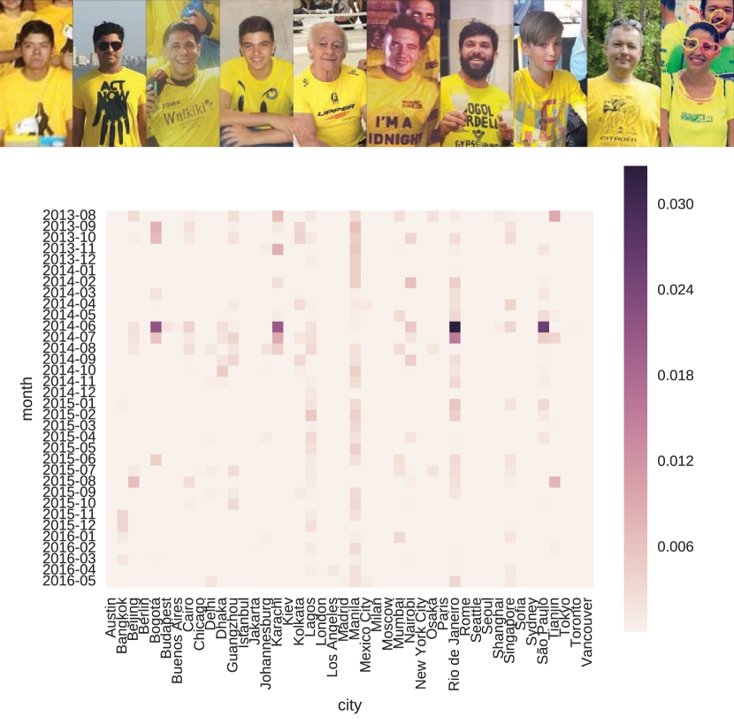
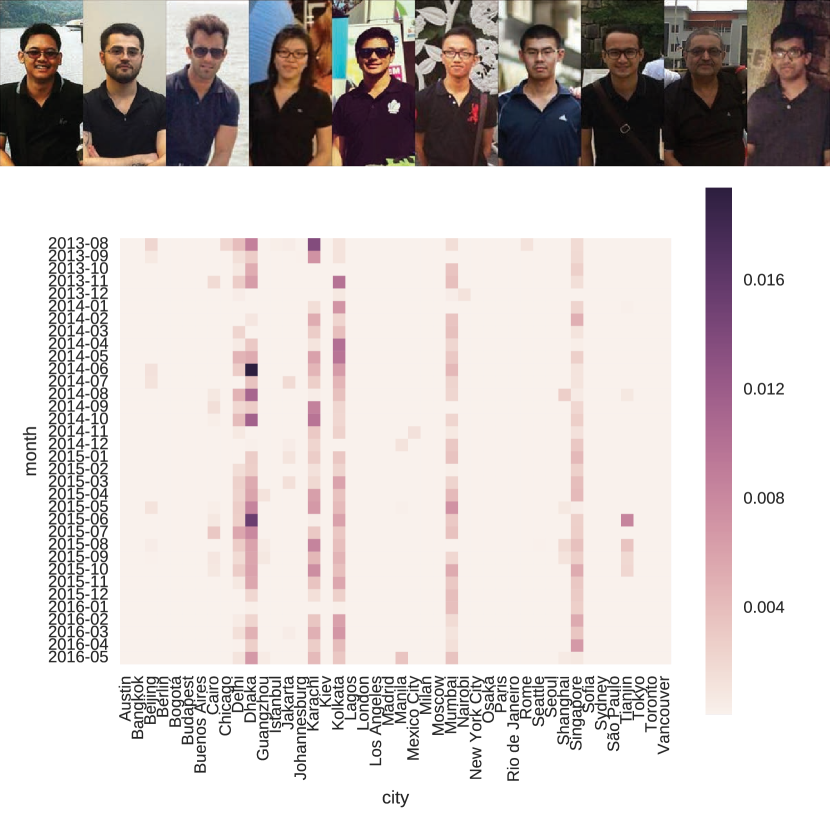
Figures 16 and 17 illustrate two other interesting top ranked clusters. Figure 16 shows that clusters can capture styles that become extremely popular at a very specific time and place, and is a variant of the yellow jersey cluster above. In this case, June and July 2014 capture the 2014 World Cup, and the contents of these clusters contain many examples of soccer fans wearing team colors. Finally, Figure 17 shows that a style that one might consider commonplace (black polo shirts with glasses) can be much more popular throughout a specific region (in this case the Indian subcontinent).
6 Conclusions and Discussion
In this work we presented a framework for analyzing clothing, style, and fashion across the world using millions of photos. Towards that end, we developed StreetStyle-27k, a large-scale, worldwide dataset of people in the wild with clothing annotations, and used this dataset to enable the analysis of a massive 15 million person photo corpus through the application of CNNs. Our work illustrates the use of machine learning and big data to perform visual discovery at scale.
Limitations. CNN-based embeddings are a very powerful approach for organizing imagery in a high-dimensional feature space. Furthermore, unsupervised methods such as GMMs can be used to further explore this space. However, there is a limit to the granularity of styles that we obtain. For instance, we do not learn a clean separation between eyeglasses and sunglasses, as those were not labeled as distinct attributes, and our style embedding does not separate those two categories. One way to discover finer-grained styles would be to incorporate active learning, where users are asked to rank similarity of styles. Another would be to apply weakly-supervised learning using the spatio-temporal metadata directly in the embedding objective function rather than using it for post hoc analysis. Finally, our method is limited to analyzing the upper body of the person. As computer vision techniques for human pose estimation mature, it would be useful to revisit this design to normalize articulated pose for full body analysis.
Future work. There are many areas for future work. We would like to more thoroughly study dataset bias. Our current dataset measures a particular population, in a particular context (Instagram users and the photos they take). We plan to extend to additional image sources and compare trends across them, but also to study aspects such as: can we distinguish between the (posed) subject of a photo and people who may be incidentally in the background? Does that make a difference in the measurements? Can we identify and take into account differences between tourists and locals? Are there certain types of people that tend to be missing from such data? Do our face detection algorithms themselves exhibit bias? We would also like to take other difficult areas of computer vision, such as pose estimation, and characterize them in a way that makes them amenable to measurement at scale.
Ultimately, we would like to apply automatic data exploration algorithms to derive, explain, and analyze the significance of insights from machine learning (e.g., see the “Automatic Statistician” [\citenameLloyd et al. 2014]). It would be also be interesting to combine visual data with other types of information, such as temperature, weather, and textual information on social media to explore new types of as-yet unseen connections. The combination of big data, machine learning, computer vision, and automated analysis algorithms, would make for a very powerful analysis tool more broadly in visual discovery of fashion and many other areas.
References
- [\citenameArietta et al. 2014] Arietta, S., Efros, A., Ramamoorthi, R., and Agrawala, M. 2014. City Forensics: Using visual elements to predict non-visual city attributes. IEEE Trans. Visualization and Computer Graphics 20, 12 (Dec).
- [\citenameBossard et al. 2013] Bossard, L., Dantone, M., Leistner, C., Wengert, C., Quack, T., and Van Gool, L. 2013. Apparel classification with style. In Proc. Asian Conf. on Computer Vision.
- [\citenameBourdev et al. 2011] Bourdev, L., Maji, S., and Malik, J. 2011. Describing people: Poselet-based attribute classification. In ICCV.
- [\citenameChen et al. 2012] Chen, H., Gallagher, A., and Girod, B. 2012. Describing clothing by semantic attributes. In ECCV.
- [\citenameCrandall et al. 2009] Crandall, D. J., Backstrom, L., Huttenlocher, D., and Kleinberg, J. 2009. Mapping the world’s photos. In WWW.
- [\citenameDi et al. 2013] Di, W., Wah, C., Bhardwaj, A., Piramuthu, R., and Sundaresan, N. 2013. Style finder: Fine-grained clothing style detection and retrieval. In Proc. CVPR Workshops.
- [\citenameDoersch et al. 2012] Doersch, C., Singh, S., Gupta, A., Sivic, J., and Efros, A. A. 2012. What makes Paris look like Paris? SIGGRAPH 31, 4.
- [\citenameDoersch et al. 2013] Doersch, C., Gupta, A., and Efros, A. A. 2013. Mid-level visual element discovery as discriminative mode seeking. In NIPS.
- [\citenameDubey et al. 2016] Dubey, A., Naik, N., Parikh, D., Raskar, R., and Hidalgo, C. A. 2016. Deep learning the city : Quantifying urban perception at a global scale. In ECCV.
- [\citenameEveringham et al. 2010] Everingham, M., Van Gool, L., Williams, C. K. I., Winn, J., and Zisserman, A., 2010. The PASCAL Visual Object Classes Challenge 2010 (VOC2010) Results. http://www.pascal-network.org/challenges/VOC/voc2010/workshop/index.html.
- [\citenameFelzenszwalb et al. 2010] Felzenszwalb, P. F., Girshick, R. B., McAllester, D., and Ramanan, D. 2010. Object detection with discriminatively trained part-based models. PAMI 32.
- [\citenameGebru et al. 2017] Gebru, T., Krause, J., Wang, Y., Chen, D., Deng, J., Lieberman Aiden, E., and Fei-Fei, L. 2017. Using Deep Learning and Google Street View to Estimate the Demographic Makeup of the US. CoRR abs/1702.06683.
- [\citenameGinosar et al. 2015] Ginosar, S., Rakelly, K., Sachs, S., Yin, B., and Efros, A. A. 2015. A Century of Portraits: A visual historical record of american high school yearbooks. In ICCV Workshops.
- [\citenameGirshick et al. 2012] Girshick, R. B., Felzenszwalb, P. F., and McAllester, D., 2012. Discriminatively trained deformable part models, release 5. http://people.cs.uchicago.edu/~rbg/latent-release5/.
- [\citenameGolder and Macy 2011] Golder, S. A., and Macy, M. W. 2011. Diurnal and seasonal mood vary with work, sleep, and daylength across diverse cultures. Science 333, 6051.
- [\citenameHe and McAuley 2016] He, R., and McAuley, J. 2016. Ups and downs: Modeling the visual evolution of fashion trends with one-class collaborative filtering. In WWW.
- [\citenameHidayati et al. 2014] Hidayati, S. C., Hua, K.-L., Cheng, W.-H., and Sun, S.-W. 2014. What are the fashion trends in new york? In Proc. Int. Conf. on Multimedia.
- [\citenameIslam et al. 2015] Islam, M. T., Greenwell, C., Souvenir, R., and Jacobs, N. 2015. Large-scale geo-facial image analysis. EURASIP J. on Image and Video Processing 2015, 1.
- [\citenameKiapour et al. 2014] Kiapour, M. H., Yamaguchi, K., Berg, A. C., and Berg, T. L. 2014. Hipster wars: Discovering elements of fashion styles. In ECCV, Springer International Publishing, Cham.
- [\citenameKiapour et al. 2015] Kiapour, M. H., Han, X., Lazebnik, S., Berg, A. C., and Berg, T. L. 2015. Where to Buy It: Matching street clothing photos in online shops. In ICCV.
- [\citenameKrizhevsky et al. 2012] Krizhevsky, A., Sutskever, I., and Hinton, G. E. 2012. ImageNet classification with deep convolutional neural networks. In NIPS.
- [\citenameLiu et al. 2012] Liu, S., Song, Z., Wang, M., Xu, C., Lu, H., and Yan, S. 2012. Street-to-shop: Cross-scenario clothing retrieval via parts alignment and auxiliary set. In Proc. Int. Conf. on Multimedia.
- [\citenameLloyd et al. 2014] Lloyd, J. R., Duvenaud, D. K., Grosse, R. B., Tenenbaum, J. B., and Ghahramani, Z. 2014. Automatic construction and natural-language description of nonparametric regression models. In AAAI.
- [\citenameMatzen and Snavely 2015] Matzen, K., and Snavely, N. 2015. Bubblenet: Foveated imaging for visual discovery. In ICCV.
- [\citenameMichel et al. 2010] Michel, J.-B., Shen, Y. K., Aiden, A. P., Veres, A., Gray, M. K., Team, T. G. B., Pickett, J. P., Holberg, D., Clancy, D., Norvig, P., Orwant, J., Pinker, S., Nowak, M. A., and Aiden, E. L. 2010. Quantitative analysis of culture using millions of digitized books. Science.
- [\citenameMurdock et al. 2015] Murdock, C., Jacobs, N., and Pless, R. 2015. Building dynamic cloud maps from the ground up. In ICCV.
- [\citenameNaik et al. 2014] Naik, N., Philipoom, J., Raskar, R., and Hidalgo, C. 2014. Streetscore: Predicting the perceived safety of one million streetscapes. In Proc. CVPR Workshops.
- [\citenameNiculescu-Mizil and Caruana 2005] Niculescu-Mizil, A., and Caruana, R. 2005. Predicting good probabilities with supervised learning. In ICML.
- [\citenamePlatt 1999] Platt, J. C. 1999. Probabilistic outputs for support vector machines and comparisons to regularized likelihood methods. In Advances in Large Margin Classifiers, MIT Press.
- [\citenameRussakovsky et al. 2015] Russakovsky, O., Deng, J., Su, H., Krause, J., Satheesh, S., Ma, S., Huang, Z., Karpathy, A., Khosla, A., Bernstein, M., Berg, A. C., and Fei-Fei, L. 2015. ImageNet Large Scale Visual Recognition Challenge. IJCV 115, 3.
- [\citenameSalem et al. 2016] Salem, T., Workman, S., Zhai, M., and Jacobs, N. 2016. Analyzing human appearance as a cue for dating images. In WACV.
- [\citenameSimo-Serra et al. 2015] Simo-Serra, E., Fidler, S., Moreno-Noguer, F., and Urtasun, R. 2015. Neuroaesthetics in fashion: Modeling the perception of fashionability. In CVPR.
- [\citenameSimonyan and Zisserman 2014] Simonyan, K., and Zisserman, A. 2014. Very deep convolutional networks for large-scale image recognition. CoRR abs/1409.1556.
- [\citenameSingh et al. 2012] Singh, S., Gupta, A., and Efros, A. A. 2012. Unsupervised discovery of mid-level discriminative patches. In ECCV.
- [\citenameSzegedy et al. 2015] Szegedy, C., Liu, W., Jia, Y., Sermanet, P., Reed, S., Anguelov, D., Erhan, D., Vanhoucke, V., and Rabinovich, A. 2015. Going deeper with convolutions. In CVPR.
- [\citenameThomee et al. 2015] Thomee, B., Shamma, D. A., Friedland, G., Elizalde, B., Ni, K., Poland, D., Borth, D., and Li, L.-J. 2015. The new data and new challenges in multimedia research. CoRR.
- [\citenamevan der Maaten and Hinton 2008] van der Maaten, L., and Hinton, G. E. 2008. Visualizing high-dimensional data using t-sne. Journal of Machine Learning Research 9.
- [\citenameVittayakorn et al. 2015] Vittayakorn, S., Yamaguchi, K., Berg, A., and Berg, T. 2015. Runway to Realway: Visual analysis of fashion. In WACV.
- [\citenameWang et al. 2013] Wang, J., Korayem, M., and Crandall, D. J. 2013. Observing the natural world with flickr. In ICCV Workshops.
- [\citenameYamaguchi et al. 2012] Yamaguchi, K., Kiapour, M., Ortiz, L., and Berg, T. 2012. Parsing clothing in fashion photographs. In CVPR.
- [\citenameYamaguchi et al. 2013] Yamaguchi, K., Kiapour, M., and Berg, T. 2013. Paper doll parsing: Retrieving similar styles to parse clothing items. In ICCV.
- [\citenameYamaguchi et al. 2015] Yamaguchi, K., Okatani, T., Sudo, K., Murasaki, K., and Taniguchi, Y. 2015. Mix and match: Joint model for clothing and attribute recognition. In BMVC.
- [\citenameYang et al. 2014] Yang, W., Luo, P., and Lin, L. 2014. Clothing co-parsing by joint image segmentation and labeling. In CVPR.
- [\citenameZhang et al. 2012] Zhang, H., Korayem, M., Crandall, D. J., and LeBuhn, G. 2012. Mining photo-sharing websites to study ecological phenomena. In WWW.
- [\citenameZhang et al. 2014] Zhang, N., Paluri, M., Rantazo, M., Darrell, T., and Bourdev, L. 2014. Panda: Pose aligned networks for deep attribute modeling. In CVPR.
- [\citenameZhu et al. 2014] Zhu, J.-Y., Lee, Y. J., and Efros, A. A. 2014. AverageExplorer: Interactive exploration and alignment of visual data collections. In SIGGRAPH.