Approximation Algorithms for Minimizing Maximum Sensor Movement for Line Barrier Coverage in the Plane

Abstract

Given a line barrier and a set of mobile sensors distributed in the plane, the Minimizing Maximum Sensor Movement problem (MMSM) for line barrier coverage is to compute relocation positions for the sensors in the plane such that the barrier is entirely covered by the monitoring area of the sensors while the maximum relocation movement (distance) is minimized. Its weaker version, decision MMSM is to determine whether the barrier can be covered by the sensors within a given relocation distance bound $D\in\mathbb{Z}^{+}$.

This paper presents three approximation algorithms for decision MMSM. The first is a simple greedy approach, which runs in time $O(n\log n)$ and achieves a maximum movement $D^{*}+2r_{max}$, where $n$ is the number of the sensors, $D^{*}$ is the maximum movement of an optimal solution and $r_{max}$ is the maximum radii of the sensors. The second and the third algorithms improve the maximum movement to $D^{*}+r_{max}$ , running in time $O(n^{7}L)$ and $O(R^{2}\sqrt{\frac{M}{\log R}})$ by applying linear programming (LP) rounding and maximal matching tchniques respecitvely, where $R=\sum 2r_{i}$, which is $O(n)$ in practical scenarios of uniform sensing radius for all sensors, and $M\leq n\max r_{i}$. Applying the above algorithms for $O(\log(d_{max}))$ time in binary search immediately yields solutions to MMSM with the same performance guarantee. In addition, we also give a factor-2 approximation algorithm which can be used to improve the performance of the first three algorithms when $r_{max}>D^{*}$. As shown in [8], the 2-D MMSM problem admits no FPTAS as it is strongly NP-complete, so our algorithms arguably achieve the best possible ratio.

I Introductions

Barrier coverage and area coverage are two important problems in applications of wireless sensor networks. In both two problems, sensors are deployed in such a way that every point of the target region is monitored by at least one sensor. For area coverage, the target region is traditionally a bounded area in the plane; while in the barrier coverage problem arising from border surveillance for intrusion detection, the target region are the borders and the goal is to deploy sensors along the borders such that at least one sensor will detect if any intruder crosses the border. Unlike area coverage, barrier coverage requires only to cover every points of the borders, rather than every point of the area bounded by the border. So barrier coverage uses much fewer sensors, and hence is more cost-efficient, particularly in practical large-scale sensor deployment.

To accomplish a barrier coverage, sensors are dispersed along the borders. However, there may exist gaps after the dispersal, so the border line might not be completely covered. One approach is to disperse the sensors in multiple rounds, and guarantee the probability of complete coverage by the dispersal density of the sensors [21, 13]. The other approach is to acquire some sensors with the ability of relocation (i.e. mobility), such that after dispersal, the sensors can move to monitor the gaps on the barrier. In this context, since the battery of a sensor is limited, a smart relocation scheme is required to maximize the lifetime of the sensors, and hence ensures a maximum lifetime of the barrier coverage.

I-A Problem Statement

This paper studies the two-dimensional (2-D) barrier coverage problem with mobile sensors, in which the barrier is modeled by a line segment, while the sensors are distributed in the plane initially. The problem is to compute the relocated positions of the sensors, such that the barrier will be completely covered while the maximum relocation distance among all the sensors is minimized.

Formally, we are given a line barrier $[0,M]$ on $x$-axis and a set of sensors distributed in the Euclidean plane, say $\Gamma=\{1,\,\dots,\,n\}$, within which sensor $i$ is with a radii $r_{i}$ and a position $(x_{i},\,y_{i})$. The two dimensional Minimum Maximum Sensor Movement problem (MMSM) is to compute the minimum $D\in\mathbb{Z}_{0}^{+}$ and a new position $(x_{i}^{\prime},\,0)$ for each sensor $i$, such that $\max_{i\in n}\sqrt{(x_{i}-x_{i}^{\prime})^{2}+(y_{i}-0){}^{2}}\leq D$ and each point on the line barrier is covered by at least one sensor (i.e. for each point on the line barrier there exists at least a sensor $i$ within distance $r_{i}$).

The paper finds that, MMSM can be reduced to a discrete version called DMMSM. In DMMSM, we are given a graph $G=(V,\,E)$, where $V=\{v_{0},\,v_{1},\,\dots,\,v_{M}\}$ and $E=\{e_{i}=(v_{i},\,v_{i+1})|i\in V\setminus\{M\}\}$. We say an edge $e_{j}$ is covered by a set of sensors $\Gamma^{\prime}\subseteq\Gamma$ if and only if every point on the edge is in the monitoring area of at least one sensor of $\Gamma^{\prime}$. The goal of DMMSM is also to compute a minimum maximum movement $D\in\mathbb{Z}_{0}^{+}$ and the new relocate position for each sensor, such that every edge of $E$ is covered by the sensors.

We propose several algorithms that are actually first to solve decision MMSM and decision DMMSM, which is to determine, for a given the relocation distance bound $D$, whether the sensors can be relocated within $D$ to cover the line barrier.

I-B Related Works

The MMSM problem in 2D setting was first studied in [8], and shown strongly ${\cal NP}$-complete for sensors with general sensing radii via a reduction from the 3-partition problem which is known strongly ${\cal NP}$-complete. Later, an algorithm with a time complexity of $O(n^{3}\log n)$ has been developed in [14] for the problem where sensors are with identical sensing radii. In the same paper, an approximation algorithm with ratio $\frac{y_{max}}{y_{min}}$ for general radii has also been developed, where $y_{max}$ and $y_{min}$ are respectively the maximum and minimum perpendicular relocation distance from the sensors to the barrier. To the best of our knowledge, there is no any other non-trivial approximation algorithm for MMSM with general radii.

Unlike 2-D MMSM, the MMSM problem has been extensively studied and well understood in 1-D setting, in which the barrier are assumed to be a line segment on the same line where the sensors are initially located. Paper [6] presented an algorithm which optimally solves 1D-MMSM for uniform radius and runs in time $O(n^{2})$, by observing the order preservation property. The time complexity was improved to $O(n\log n)$ later in paper [5], which also gave an $O(n^{2}\log n)$ time algorithm for general radii. Recently, an $O(n^{2}\log n\log\log n)$ time algorithm has been presented in [19] for weighted 1D-MMSM with uniform radii, in which each sensor has a weight, and the moving cost of a sensor is its movement times its weight. Moreover, circle/simple polygon barriers has been studied besides straight lines in [3], in which two algorithms has been developed for MMSM, with an $O(n^{3.5}\log n)$ time against cycle barriers and an $O(mn^{3.5}\log n)$ time against polygon barriers, where $m$ is the number of the edges on the polygon. The later time complexity was then improved to $O(n^{2.5}\log n)$ in [18].

Other problems closely related to MMSM have also been well studied in previous literature. In 1-D setting, the Min-Sum relocation problem, to minimize the sum of the relocation distances of all the sensors, is shown ${\cal NP}$-complete for general radii while solvable in time $O(n^{2})$ for uniform radii [7]. The Min-Num relocation problem of minimizing the number of sensors moved, is also proven ${\cal NP}$-complete for general radii and polynomial solvable for uniform radii [16]. Similar to MMSM, where a PTAS has been developed for the Min-Sum relocation problem against circle/simple polygon barriers [3], which was improved by later paper [18] that gave an $O(n^{4})$ time exact algorithm.

Paper [1] studied a more complicated problem of maximizing the coverage lifetime, in which each mobile sensor is equipped with limited battery power, and the coverage lifetime is the time to when the coverage no longer works because of the death of a sensor. The authors presented parametric search algorithms for the cases when the sensors have a predetermined order in the barrier or when sensors are initially located at barrier endpoints. On the other hand, the same authors present two FPTAS respectively for minimizing sumed and maximum energy consumption when the radii of the sensors can be adjusted [2]. When the sensing radii is fixed, i.e. unadjustable, the same paper showed the min-sum problem can not be approximated within $O(n^{c})$ for any constant $c$ under the assumption of ${\cal P}\neq{\cal NP}$, while the min-max version is known strongly ${\cal NP}$-complete, as it can be reduced to 2-D MMSM which is know strongly ${\cal NP}$-complete [8].

Before deployment of mobile sensors, barrier coverage was first considered deploying stationary sensors [12] for covering a closed curve (i.e. a moat), and an elegant algorithm was proposed by transferring the Min-Sum cost barrier coverage problem to the shortest path problem. It has then been extensively studied for line based employment [17], for better local barrier coverage [4], and for using camera sensors [20, 15]. The most recent result [9] studied line barrier coverage using sensors with adjustable sensing ranges. They show the problem is polynomial solvable when each sensor can only choose from a finite set of sensing ranges, and ${\cal NP}$-complete if each sensor can choose any sensing ranges in a given interval.

I-C Our Results and Technique

In this paper, we present two approximation algorithms for the decision MMSM problem. The first is a simple greedy approach based on our proposed sufficient condition of determining whether there exists a feasible cover for the barrier under the relocation distance bound $D$. If $D<D^{*}$, the algorithm outputs “infeasible”; Otherwise, the algorithm computes new positions for the sensors, resulting a maximum relocation distance $D+2r_{max}$, where $r_{max}=\max_{i}\{r_{i}\}$. The algorithm is so efficient that it runs in time $O(n\log n)$, where $n=|\Gamma|$ is the number of the sensors. The second is generally an linear programming (LP) rounding based approach, which first transfers MMSM to the fractional cardinality matching problem and then solves the LP relaxation we propose for the latter problem. The algorithm approximately solves the decision MMSM problem according to a solution to the LP relaxation. Similar to the case for the first algorithm, we show that the algorithm always outputs “feasible” if $D\geq D^{*}$. Further, for any instance our algorithm returns “feasible”, we give a method to construct a real solution for MMSM, with a maximum relocation distance $D+r_{max}$, by rounding up a fractional optimum solution to the LP relaxation. The algorithm has a runtime $O(n^{7}L)$, which is exactly the time of solving the proposed LP relaxation by Karmakar’s algorithm [10], where $L$ is the length of the input. As a by-product, we give the third algorithm for decision MMSM with a maximum relocation distance $d(OPT)+r_{max}$, and time $O(R^{2}\sqrt{\frac{M}{\log R}})$, where $R=\sum_{i=1}^{n}2r_{i}$ is sum of the radii of the sensors.

Based on the three above algorithms for the decision problem, the paper proposes an unified algorithm framework to actually calculate a solution to MMSM without a given $D$. The time complexity and the maximum relocation distance are respectively $O(n\log n\log d_{\max})$ and $D^{*}+2r_{max}$ if employing the greedy algorithm; $O(n^{7}L\log d_{max})$ and $D^{*}+r_{max}$ if employing the LP based algorithm, where $d_{max}$ is the maximum distance between the sensors and the barriers. The runtime $O(n^{7}L\log d_{max})$ can be improved to $O(R^{2}\sqrt{\frac{M}{\log R}}\log d_{max})$ if $M$ is not large, by using the third algorithm based on matching.

Note that, although our algorithm could compute a near-optimal solution when $D^{*}\gg r_{max}$, the performance guarantee is not as good when $D^{*}<r_{max}$. So in addition we give a simple factor-2 approximation algorithm for MMSM, by extending the optimal algorithm for 1D-MMSM as in paper [5]. Consequently, the ratio of our first three algorithms can be improved for the case $D^{*}<r_{max}$, by combining the factor-2 approximation.

I-D Organization of the Paper

The remainder of the paper is organized as follows: For decision MMSM, Section 2 gives a greedy algorithm as well as the ratio proof; Section 3 gives an approximation algorithm with an improved maximum relocation distance $d(OPT)+r_{max}$ using LP rounding technique; Section 4 gives another approximation algorithm with the same maximum relocation distance guarantee but a different runtime, by using maximum cardinality matching; Section 5 present the algorithm which actually solve MMSM, using the algorithm given in Section 2, 3 and 4; Section 6 extends previous results and develops a factor-2 approximation algorithm with provable performance guarantee; Section 7 concludes the paper.

II A Simple Greedy Algorithm For Decision MMSM

This section presents an approximation algorithm for any instance of decision MMSM wrt a given $D$: if the algorithm returns “infeasible”, then the instance is truly infeasible with respect to $D$; Otherwise, the instance of MMSM is feasible under the maximum movement of $D+2r_{max}$, where $r_{max}=\max_{i}\{r_{i}\}$. To show the performance guarantee of the algorithm, we propose a sufficient condition for the feasibility of decision MMSM against given $D$.

II-A An Approximation Algorithm

Let $[l_{i},\,g_{i}]$ be the possible coverage range for sensor $i$, where $l_{i}$ and $g_{i}$ are respectively the leftmost and the rightmost points of the barrier, i.e. the leftmost and the rightmost points sensor $i$ can cover by relocating within distance $D$. The key idea of our algorithm is to cover the barrier from left to right, using the sensor with minimum $g_{i}$ within the set of sensors which can cover the leftmost uncovered point with a maximum relocation distance $D+2r_{max}$.

More detailed, the algorithm is first to compute for each sensor $i$ its possible coverage range $[l_{i},\,g_{i}]$. Let $s$ be the leftmost point of the uncovered part of the line barrier. Then among the set of sensors $\{i|l_{i}-2r_{max}\leq s\leq g_{i}\}$, the algorithm repeats selecting the sensor with minimum $g_{i}$ to cover an uncovered segment of the line barrier starting at $s$. Note that $\{i|l_{i}-2r_{max}\leq s\leq g_{i}\}$ is exactly the set of sensors, which are with $g_{i}\geq s$ and can monitor an uncovered segment starting at $s$ by relocating at most $D+2r_{max}$ distance. If there is a tie on $g_{i}$, then randomly pick a sensor within the tie. The selection terminates once the line barrier is completely covered, or the instance is found infeasible, i.e. there exists no such $i$ with $l_{i}-2r_{max}\leq s\leq g_{i}$ while the coverage is not done. The algorithm is formally as in Algorithm 1.

Input: A movement distance bound $D\in\mathbb{Z}^{+}$, a set of sensors $\Gamma=\{1,\,\dots,\,n\}$ with $\{r_{i}|i\in[n]^{+}\}$ and $\{(x_{i},\,y_{i})|i\in[n]^{+}\}$, in which $r_{i}$ and $(x_{i},\,y_{i})$ are respectively the sensing radii and the original position of sensor $i$;

Output: New positions $\{(x_{i}^{\prime},\,y_{i}^{\prime})|i\in[n]^{+}\}$ for the sensors.

1: Set ${\cal I}:=\Gamma$, $s:=0$; /*$s$ is the leftmost point of the uncovered part of the barrier.*/

2: For each sensor $i$ do

3:  Compute the leftmost position $l_{i}$ and the rightmost position $g_{i}$, both of which sensor $i$ can monitor;

4: While ${\cal I}\neq\emptyset$ do

5:  If there exists $i^{\prime}\in{\cal I}$, such that $l_{i^{\prime}}-2r_{max}\leq s\leq g_{i^{\prime}}$ then

6:   Select $i\in{\cal I}$ for which $g_{i}=\min_{i^{\prime}:\,l_{i^{\prime}}-2r_{max}\leq s\leq g_{i^{\prime}}}\{g_{i^{\prime}}\}$;

/* Select the sensor with minimum $g_{i}$ among the sensors $\{i^{\prime}|l_{i^{\prime}}-2r_{max}\leq s\}$; */

7:   Set $s:=\min\{s+2r_{i},\,g_{i}\}$, ${\cal I}:={\cal I}\setminus\{i\}$, $x_{i}^{\prime}:=s-r_{i}$, $y_{i}^{\prime}:=0$;

8:  Else

9:   Return “infeasible”.

10: Return “feasible” the new positions $\{(x^{\prime}_{i},\,0)|i\in[n]^{+}\}$.

Algorithm 1 A simple greedy algorithm for decision MMSM.

For briefness, we will simply say an instance (or the input) of MMSM instead for the input of Algorithm 1 in the following paragraphs. Note that Steps 2-3 take time $O(n)$ to compute $l_{i}$ and $g_{i}$ for all the sensors, Steps 4-7 take $O(n\log n)$ time to assign the sensors to cover the line barrier. Therefore, we have the time complexity of the algorithm:

Lemma 1.

Algorithm 1 runs in time $O(n\log n)$.

II-B The Ratio of Algorithm 1

The performance guarantee of Algorithm 1 is as below:

Theorem 2.

Let $D^{*}$ be the distance of an optimal solution. If $D\geq D^{*}$, then Algorithm 1 will return a solution with maximum relocation distance $D+2r_{max}$, where $r_{max}=\max_{i}\{r_{i}\}$.

According to Algorithm 1, we never move a sensor out of the range $[l_{i}-2r_{max},\,g_{i}]$. It remains to show Algorithm 1 will always return a feasible solution when $D\geq D^{*}$. For this goal, we will give a sufficient condition for the feasibility of decision MMSM. Below are two notations needed for the tasks:

$$\lambda(i,\,D,\,x,\,x^{\prime})=\begin{cases}0&g_{i}\leq x\,\mbox{or}\,l_{i}\geq x^{\prime}\\ \min\{2r_{i},\,\min\{x^{\prime},\,g_{i}\}-\max\{x,\,l_{i}\}\}&Otherwise\end{cases}$$

and

$$\sigma(i,\,D,\,{\cal S})=\begin{cases}0&g_{i}\leq x\,\mbox{OR}\,l_{i}\geq x^{\prime}\\ \min\{2r_{i},\,\sum_{[x,x^{\prime}]\in{\cal S}}\lambda(i,\,D^{*},\,x,\,x^{\prime})\}&Otherwise\end{cases}$$

where ${\cal S}$ is a set of disjoint segments of the line barrier. Intuitionally $\lambda(i,\,D,\,x,\,x^{\prime})$ is the maximum coverage which sensor $i$ can provide for segment $[x,\,x^{\prime}]$, and $\sigma(i,\,D,\,{\cal S})$ is the sum of the coverage that sensor $i$ can provide for all the segments in ${\cal S}$. Then a simple necessary condition for the feasibility of an instance of MMSM of as below:

Proposition 3.

If an instance of decision MMSM is feasible wrt $D$, then $\sum_{i}\sigma(i,\,D,\,{\cal S})\geq\sum_{[x_{j},\,x_{j}^{\prime}]\in{\cal S}}|x_{j}^{\prime}-x_{j}|$ must hold for any set of disjoint segments ${\cal S}=\{[x_{i},\,x_{i}^{\prime}]|0\leq i\leq M\}$.

Intuitionally, the above proposition states that the sum of the sensor coverage length must be not less than the length of the barrier segments to cover. The correctness of the above lemma is obviously, since a feasible relocation assignment must satisfy the condition. However, this is not a sufficient condition for the feasibility of decision MMSM (A counter example is as depicted in Figure 2 (a): For $D=r_{1}$, the necessary condition holds for the given instance while the instance is actually infeasible). However, if $2r_{max}$ more relocation distance is allowed as in Algorithm 1, we have the following lemma:

Lemma 4.

If $\sum_{i}\sigma(i,\,D,\,{\cal S})\geq\sum_{[x_{j},\,x_{j}^{\prime}]\in{\cal S}}|x_{j}^{\prime}-x_{j}|$ holds for every disjoint segments set ${\cal S}$, then the instance of decision MMSM is feasible under maximum relocation distance $D+2r_{max}$, $r_{max}=\max_{i}\{r_{i}\}$.

Proof:

We need only to show that if $\sum_{i}\sigma(i,\,D,\,{\cal S})\geq\sum_{[x_{j},\,x_{j}^{\prime}]\in{\cal S}}|x_{j}^{\prime}-x_{j}|$ holds at the beginning of Algorithm 1, then $\sum_{i}\sigma(i,\,D,\,{\cal S})\geq\sum_{[x_{j},\,x_{j}^{\prime}]\in{\cal S}}|x_{j}^{\prime}-x_{j}|$ remains true in each step of Algorithm 1.

Suppose the lemma is not true. Let the step of picking sensor $i$ be the first $\sum_{i}\sigma(i,\,D,\,{\cal S})\geq\sum_{[x_{j},\,x_{j}^{\prime}]\in{\cal S}}|x_{j}^{\prime}-x_{j}|$ becomes false. Then there must exist $x$ and $x^{\prime}$, such that $\sum_{j\in{\cal I}}\sigma(j,\,D,\,x,\,x^{\prime})\geq|x^{\prime}-x|$ and $\sum_{j\in{\cal I}\setminus i}\sigma(j,\,D,\,x,\,x^{\prime})<|x^{\prime}-x|$. We analysis all cases wrt all the possible orders of $g_{i}$, $s+2r_{i}$ and $x$ in the line barrier, and show that contradictions exist in every case.

1. $g_{i}\leq x$:

   In this case, $\sigma(i,\,D,\,[x,\,x^{\prime}])=0$ holds, i.e. sensor $i$ does not cover any portion of $[x,\,x^{\prime}]$. So we have

   $$\sum_{j\in{\cal I}\setminus\{i\}}\sigma(j,\,D,\,x,\,x^{\prime})=\sum_{j\in{\cal I}}\sigma(j,\,D,\,[x,\,x^{\prime}])\geq|x^{\prime}-x|,$$

   which contradicts with $\sum_{j\in{\cal I}\setminus\{i\}}\sigma(j,\,D,\,[x,\,x^{\prime}])<|x^{\prime}-x|$.

2. $x<g_{i}\leq s+2r_{i}$:

   In this case, sensor $i$ will actually cover $[s,\,s+2r_{i}]$, and hence $\sigma(i,\,D,\,[x,\,x^{\prime}])=\min\{g_{i},\,x^{\prime}\}-x$ is the actual coverage that sensor $i$ can contribute to $\sum_{j\in{\cal I}}\sigma(j,\,D,\,[x,\,x^{\prime}])$. So

   $$\sum_{j\in{\cal I}\setminus\{i\}}\sigma(j,\,D,\,[x,\,x^{\prime}])=\sum_{j\in{\cal I}}\sigma(j,\,D,\,[x,\,x^{\prime}])-(\min\{g_{i},\,x^{\prime}\}-x).$$ (1)

   Then by combining $\sum_{j\in{\cal I}}\sigma(j,\,D,\,x,\,x^{\prime})\geq x^{\prime}-x$ with Inequality (1), we have

   $$\sum_{j\in{\cal I}\setminus\{i\}}\sigma(j,\,D,\,[x,\,x^{\prime}])\geq x^{\prime}-x-(\min\{g_{i},\,x^{\prime}\}-x)=x^{\prime}-\min\{g_{i},\,x^{\prime}\}$$ (2)

   On the other hand, the length of the portion of $[x,\,x^{\prime}]$ that needs to be covered is apparently $|x^{\prime}-x|-(\min\{g_{i},\,x^{\prime}\}-x)$. From the infeasibility of the remaining sensors in ${\cal I}$, we have

   $$\sum_{j\in{\cal I}\setminus\{i\}}\sigma(j,\,D,\,[x,\,x^{\prime}])<x^{\prime}-x-(\min\{g_{i},\,x^{\prime}\}-x)=x^{\prime}-\min\{g_{i},\,x^{\prime}\}.$$ (3)

   A contradiction arises by comparing Inequality (2) and (3).

3. $g_{i}>x$ and $g_{i}>s+2r_{i}$:

   Assume that $s+2r_{i}\leq x$. This assumption is without loss of generality, since otherwise from $\sum_{j\in{\cal I}\setminus\{i\}}\sigma(j,\,D,\,x,\,x^{\prime})<|x^{\prime}-x|$ and the fact that $[x,\,s+2r_{i}]$ is already covered by sensor $i$, we have $\sum_{j\in{\cal I}\setminus\{i\}}\sigma(j,\,D,\,s+2r_{i},\,x^{\prime})<x^{\prime}-(s+2r_{i})$. That is, we need only to set $x=s+2r_{i}$, and obtain contractions similar as this case. We will show that $\sum_{j\in{\cal I}\setminus\{i\}}\sigma(j,\,D,\,s+2r_{i},\,x^{\prime})\geq x^{\prime}-(s+2r_{i})$ actually holds and get a construction

   By inductions, we have

   $$\sum_{j\in{\cal I}}\sigma(j,\,D,\,\{[s,\,s+2r_{i}],\,[x,\,x^{\prime}]\})\geq 2r_{i}+x^{\prime}-x.$$

   That is,

   $$\sum_{j\in{\cal I}}\sigma(j,\,D,\,\{[s,\,s+2r_{i}],\,[x,\,x^{\prime}]\})-2r_{i}\geq x^{\prime}-x.$$

   So

   $$\sum_{j\in{\cal I}\setminus\{i\}}\sigma(j,\,D,\,\{[s,\,s+2r_{i}],\,[x,\,x^{\prime}]\})\geq x^{\prime}-x.$$ (4)

   Assume that sensor $j\neq i$ is a sensor which can contribute to both $\sigma(j,\,D,\,[s,\,s+2r_{i}])$ and $\sigma(j,\,D,\,[x,\,x^{\prime}])$. Let $\phi(j,\,D,\,[s,\,s+2r_{i}])$ and $\phi(j,\,D,\,[x,\,g_{i}])$ be the portion that sensor $j$ actually contributes $[s,\,s+2r_{i}]$ and $[x,\,g_{i}]$, respectively, within $\sum_{j\in{\cal I}}\sigma(j,\,D,\,([s,\,s+2r_{i}],\,[x,\,x^{\prime}]))$. We need only to show that $\sum_{j\in{\cal I}\setminus\{i\}}\phi(j,\,D,\,[s,\,s+2r_{i}])$ is sufficient to be relocated to compensate all the coverage sensor $i$ contributes to $[x,\,g_{i}]$.

   Since the chosen sensor $i$ is with smallest $g_{i}$ within all the sensors of $l_{i}-2r_{max}\leq s$, sensor $j\in{\cal I}\setminus\{i\}$ is with $g_{j}\geq g_{i}$. So the potion of sensor $j$ covering $[s,\,s+2r_{i}]$, i.e. $\phi(j,\,D,\,[s,\,s+2r_{i}])$, can all be relocated to cover any portion of $[x,\,g_{i}]$. So $\phi(j,\,D,\,[s,\,s+2r_{i}])+\phi(j,\,D,\,[x,\,\min\{g_{i},\,x^{\prime}\}])$ is actually the portion of the cover that sensor $j$ can contributes to $[x,\,g_{i}]$. Therefore, we have

   $$\sum_{j\in{\cal I}\setminus\{i\}}\sigma(j,\,D,\,[x,\,x^{\prime}]) = \sum_{j\in{\cal I}\setminus\{i\}}(\phi(j,\,D,\,[s,\,s+2r_{i}])$$ (5)

   $$+\phi(j,\,D,\,[x,\,\min\{g_{i},\,x^{\prime}\}]) + \sum_{j\in{\cal I}\setminus\{i\}}\phi(j,\,D,\,[\min\{g_{i},\,x^{\prime}\},\,x^{\prime}]\}).$$

   On the other hand, we have

   $$\sum_{j\in{\cal I}\setminus\{i\}}\sigma(j,\,D,\,\{[s,\,s+2r_{i}],\,[x,\,x^{\prime}]\}) \leq\sum_{j\in{\cal I}\setminus\{i\}}\phi(j,\,D,\,[s,\,s+2r_{i}])$$ (6)

   $$+ \sum_{j\in{\cal I}\setminus\{i\}}\phi(j,\,D,\,[x,\,\min\{g_{i},\,x^{\prime}\}]) +\sum_{j\in{\cal I}\setminus\{i\}}\phi(j,\,D,\,[\min\{g_{i},\,x^{\prime}\},\,x^{\prime}]\}).$$

   Combining Inequality (4), (5) and (6), we have $\sum_{j\in{\cal I}\setminus\{i\}}\sigma(j,\,D,\,[x,\,x^{\prime}])\geq\sum_{j\in{\cal I}\setminus\{i\}}\sigma(j,\,D,\,\{[s,\,s+2r_{i}],\,[x,\,x^{\prime}]\})\geq x^{\prime}-x$, which contradicts with the assumption.

∎

Now we will prove Theorem 2. If $D\geq D^{*}$, then the decision MMSM is feasible, and hence following Proposition 3 $\sum_{i}\sigma(i,\,D,\,{\cal S})\geq\sum_{[x_{j},\,x_{j}^{\prime}]\in{\cal S}}|x_{j}^{\prime}-x_{j}|$ holds for every ${\cal S}$ at the beginning of Algorithm 1. Then from Lemma 4, we immediately have the instance is feasible under relocation distance bound $D$, which completes the proof of Theorem 2.

Corollary 5.

The performance guarantee of Algorithm 1 in Theorem 2 is nearly tight.

As the example depicted in Figure 1, $d(OPT)=2r_{1}$ while the output of the algorithm is with a maximum relocation distance $2r_{2}$. So when $r_{2}\gg r_{1}$, $d(OPT)+2r_{max}\thickapprox 2r_{1}+2r_{2}$, and hence the analysis of Algorithm 1 is nearly tight in Theorem 2.

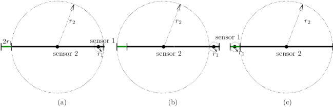
Figure 1: A near-tight example for Algorithm 1: (a) An instance of decision MMSM: line barrier is between points $(0,\,0)$ and $(2r_{1}+2r_{2},\,0)$, while the positions of sensor 1 and 2 are respectively $(2r_{2}+r_{1},\,0)$ and $(2r_{1}+r_{2},\,0)$; (b) The optimal solution with maximum relocation distance $2r_{1}$; (c) The solution output by Algorithm 1 with maximum relocation distance $2r_{2}$.

III An LP-based Approximation for Decision MMSM

This section will give an LP-based approximation algorithm to determine whether an instance of the decision MMSM problem is feasible. The algorithm first transfers the instance to a corresponding instance of decision DMMSM, and then an instance of the fractional cardinality matching problem with a proposed LP relaxation. Our algorithm answers “feasible” or “infeasible” according to the computed optimum solution of the LP relaxation. We show that if our algorithm returns feasible, then a solution to MMSM can be constructed under the maximum relocation distance $D+r_{max}$ by rounding up a fractional optimum solution to the relaxation.

III-A Transferring to an Instance of DMMSM

The key idea of the transfer is first to compute $l_{i}$ and $g_{i}$ for each $i$ wrt to the given $D$, and then add $(l_{i},\,0)$ and $(g_{i},\,0)$ to the barrier as two vertices on the line. That is, $V=\{(l_{i},\,0)|i\in[n]^{+}\}\cup\{(g_{i},\,0)|i\in[n]^{+}\}$. W.l.o.g. assume that the vertices of $V$ appear on the line barrier in the order of $v_{0},\,\dots,\,v_{|V|}$, from left to right on the line barrier. Then the algorithm adds an edge between every pair of $v_{i}$ and $v_{i+1}$. So $E=\{e_{i}(v_{i},\,v_{i+1})|i\in[|V|-1]^{+}\}$. Formally the transfer is as in Algorithm 2.

Input: An instance of MMSM;

Output: $G=(V,\,E)$, an instance of DMMSM.

1: Set $V:=\emptyset$ and $E:=\emptyset$;

2: For each edge $i\in S$ do

3:  Compute $l_{i}$ and $g_{i}$;

4:  $V\leftarrow V\cup\{(l_{i},\,0),\,(g_{i},\,0)\}$;

5: Number the vertices of $V$, such that the vertices appear in the barrier from left to right in the order of $v_{0},\,\dots,\,v_{|V|}$;

6: Set $E:=\{e_{j}(v_{j},\,v_{j+1})|j\in[|V|-1]^{+}\}$;

7: Return $G=(V,\,E)$.

Algorithm 2 The transferring algorithm.

For the time complexity and the size of the graph, we have:

Lemma 6.

Algorithm 2 runs in $O(n\log n)$ time, and output a graph $G$ with $|V|=O(n)$ and $|E|=O(n)$.

According to the algorithm, $|V|=O(n)$ and $|E|=O(n)$ hold trivially. Algorithm 2 takes in $O(n\log n)$ time to sort (number) the vertices of $V$ in Step 5, since $|V|=O(n)$. Other steps of the algorithm takes trivial time compared to the sorting. So the total runtime of Algorithm 2 is $O(n\log n)$.

Lemma 7.

An instance of MMSM is feasible under $D$ if and only if its corresponding DMMSM instance produced by Algorithm 2 is feasible under $D$.

Proof:

According to Algorithm 2 and following the definition of MMSM and DMMSM, a solution to an instance of MMSM is obviously a solution to the corresponding instance of DMMSM, and vice versa. So an instance of MMSM is feasible, iff its corresponding DMMSM instance is feasible. ∎

III-B Fractional Maximum Cardinality Matching wrt DMMSM

Let $|e_{i}|=v_{i+1}-v_{i}$ be the length of edge $e_{i}$. Assuming that $v_{i_{1}}=l_{i}$ and $v_{i_{2}}=g_{i}$, we set $J_{i}=\{e_{j}|j=i_{1},\,i_{1}+1,\,\dots,\,i_{2}-1\}$. Then the linear programming relaxation (LP1) for DMMSM is as below:

$$\max\sum_{i\in[n]^{+}}\sum_{j\in J_{i}}x_{i,\,j}$$

subject to

$$\sum_{j\in J_{i}}x_{i,j} \leq 2r_{i} \forall i\in\{1,\,\dots,\,n\}$$ (7)

$$\sum_{i\in[n]^{+}}x_{i,\,j} \leq|e_{j}| \forall j\in\{1,\,\dots,\,|V|\}$$ (8)

$$0\leq x_{i,\,j} \leq|e_{j}| \forall i\in\{1,\,\dots,\,n\},\,j\in J_{i}$$ (9)

where $\sum_{j\in J_{i}}x_{i,j}\leq 2r_{i}$ is because a sensor $i$ can at most cover length $2r_{i}$ of the barrier, and Inequality (8) is because the covered length of each edge $e_{i}$ (segment) is at most $|e_{j}|$.

Our algorithm determines decision DMMSM according to the computed optimum solution, say $\mathbf{x}$, to LP1: the algorithm outputs “feasible” if $\sum_{i\in[n]^{+}}\sum_{j\in J_{i}}x_{i,\,j}=M$, and outputs “infeasible” otherwise.

Input: An instance of DMMSM;

Output: Answer whether the instance is feasible.

1: Solve LP1 against the instance of DMMSM by Karmakar’s algorithm as in [10], and obtain an optimal solution $\mathbf{x}$;

2: If $\sum_{i\in[n]^{+}}\sum_{j\in J_{i}}x_{i,\,j}=M$ according to $\mathbf{x}$ then

3:  Return “feasible”;

4: else

5:  Return “infeasible”;

Algorithm 3 The determining algorithm for decision DMMSM.

It is known that there exist polynomial-time algorithms for solving linear programs. In particular, using Karmakar’s algorithm to solve LP1 will take $O(n^{7}L)$ time [10], since there are $O(n^{2})$ variables totally in LP1.

Lemma 8.

Algorithm 3 runs in time $O\left(n^{7}L\right)$.

It is worth to note that the simplex algorithm has a much better practical performance than Karmakar’s algorithm [11]. So using the simplex method the algorithm would be faster than $O(n^{7}L)$ in real world applications.

The performance guarantee of Algorithm 3 is as given in the following theorem, whose proof will be given in next subsection.

Theorem 9.

If Algorithm 3 returns “infeasible”, then the instance of DMMSM is truly infeasible under the given $D$; Otherwise, the instance of DMMSM is truly feasible under the maximum relocation distance $D+r_{max}$, where $r_{max}=\max_{i}\{r_{i}\}$.

Corollary 10.

The performance guarantee given in Theorem 9 is nearly tight for Algorithm 3.

From Figure 2, an optimal fractional solution to LP1 is with a maximum relocation distance $r_{1}$, while a true optimal solution for MMSM must be with a maximum relocation distance $r_{2}$. Thus, the integral gap for LP1 is $r_{2}-r_{1}\approx r_{max}$ when $r_{2}\gg r_{1}$. That is, for any fixed $\epsilon>0$, the maximum relocation distance increment could be larger than $r_{max}-\epsilon$ for rounding an optimum solution of LP1 to a true solution of MMSM. Therefore, the ratio is nearly-tight for Algorithm 3.

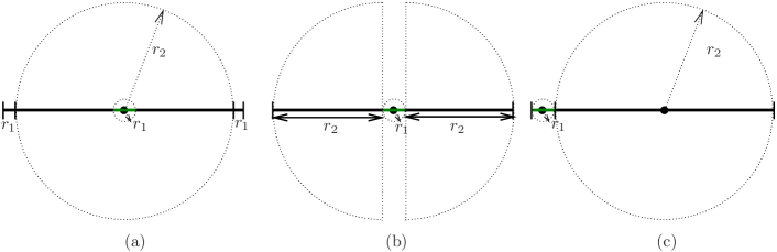
Figure 2: The integrality gap: (a) An instance of decision MMSM: line barrier is between points $(0,\,0)$ and $(2r_{1}+2r_{2},\,0)$, while the positions of sensor 1 and 2 are both $(r_{1}+r_{2},\,0)$; (b) Algorithm 3 outputs “feasible” if $D\geq r_{2}$; (c) The optimal maximum relocation distance is actually $r_{1}$.

III-C Proof of Theorem 9

This subsection will prove Theorem 9 by showing a fractional optimum solution to LP1 can be rounded up to an integral solution of DMMSM with a maximum relocation distance $D+r_{max}$.

Let $\mathbf{x}$ be an optimum solution to LP1. Recall that $x_{ij}$ is the (fractional) portion sensor $i$ covering edge $j$, the key idea of our algorithm is to aggregate the portions of sensor $i$ covering different $j$s, such that the portions combine to a line segment which $i$ can cover within movement $D+r_{max}$.

Our algorithm is composed by two parts. The first part is called pre-aggregation which rounds $x_{ij}$ to $1$ in a “pseudo” way. More precisely, assume that $0<x_{i_{1},\,j},\,\dots,\,x_{i_{h},\,j}<0$ are the variables shares edge $e_{j}$. Then the pre-aggregation divides $e_{j}$ to a set of sub-edges $\{e_{j,\,i_{1}},\,\dots,e_{j,\,i_{h}}\}$, in which $|e_{j,\,i_{l}}|=|e_{j}|\cdot x_{i_{l},\,j}$. We set $x_{i_{l},\,j,\,l}=1$, which is, edge $e_{j,\,i_{l}}$ completely covered by sensor $i_{l}$.

Let ${\cal S}_{i}$ be the set of sub-edges covered by sensor $i$ accordingly. The second part, which is called aggregation, aggregates the edges of ${\cal S}_{i}$ for each $i$ such that the edges covered by an identical sensor will connect together. The aggregation starts from the following simple observation whose correctness is obviously:

Proposition 11.

Let $i$ and $i^{\prime}$ be two sensors. Let ${\cal S}_{i}$ and ${\cal S}_{i}^{\prime}$ be the set of edges covered by sensor $i$ and $i^{\prime}$, respectively. Then, for any sub-edges $j_{1},\,j_{2}\in{\cal S}_{i}$ and $j_{1}^{\prime},\,j_{2}^{\prime}\in{\cal S}_{i^{\prime}}$, w.l.o.g. assuming $j_{1}<j_{1}^{\prime}$, $j_{1}<j_{2}$ and $j_{1}^{\prime}<j_{2}^{\prime}$, then exactly one of the following cases holds: (1) $j_{1}<j_{2}<j_{1}^{\prime}<j_{2}^{\prime}$ ; (2) $j_{1}<j_{1}^{\prime}<j_{2}<j_{2}^{\prime}$ ; (3) $j_{1}<j_{1}^{\prime}<j_{2}^{\prime}<j_{2}$.

The key observation of the aggregation is that if case (2) and (3) in the above proposition can be eliminated, then the set of edges in ${\cal S}_{i}$ are aggregated together that they can be truly monitored by sensor $i$. So the aggregation is accordingly composed by two phases called the swap phase and the exchange step, which are to eliminate case (2) and (3), respectively. Formally, the algorithm is as in Algorithm 4 (An example of such rounding depicted as in Figure 3 and 4).

Figure 3: An instance of decision MMSM: Sensors 1, 2 and 3 are with identical sensing radii $r$, and positions $(3r,\,0)$, $(3r,\,-1.2r)$, $(3r,\,2r)$, respectively. The barrier to cover is $[0,\,6r]$ and the given $D=2r$.

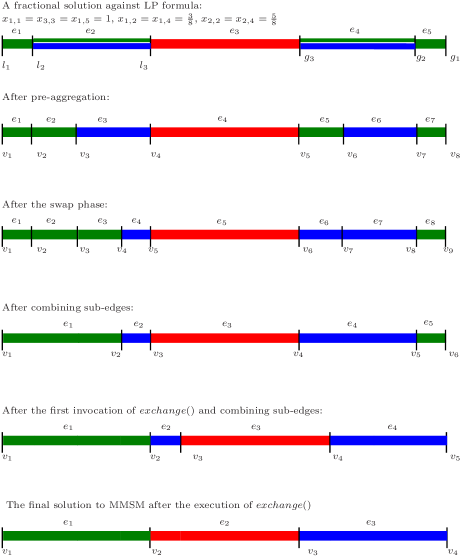
Figure 4: Execution of Algorithm 4 against the instance as in Figure 3.

Input: $\mathbf{x}$, an optimum solution to LP1 with $\sum_{i\in[n]^{+}}\sum_{j\in J_{i}}x_{i,\,j}=M$;

Output: Relocate positions for the sensors.

1: Run pre-aggregation: compute ${\cal S}_{i}$ for each sensor $i$ according to $\mathbf{x}$;

/*${\cal S}_{i}$ contains the sub-edges covered by sensor $i$. */

2: Set ${\cal S}=\{{\cal S}_{i}|i\in[n]^{+}\}$;

3: Swap(${\cal S}$); /*The swap phase.*/

4: Combine every pairs of adjacent edges for each ${\cal S}_{i}\in{\cal S}$;

5: Exchange (${\cal S}$); /*The exchange step. */

6: For $i=1$ to $n$ do

Compute $(x_{i}^{\prime},\,0)$ such that every sub-edge of ${\cal S}_{i}$ is with the range $[x_{i}^{\prime}-r_{i},\,x_{i}^{\prime}+r_{i}]$ while $\sqrt{(x_{i}^{\prime}-x_{i})^{2}+y_{i}^{2}}$ attains minimum;

7: Return $\{(x^{\prime}_{i},\,0)|i=1,\,\dots,\,n\}$.

Algorithm 4 An approximation algorithm for rounding an optimum solution to LP1.

Note that if two adjacent sub-edges belong to the same ${\cal S}_{i}$, say $e_{j_{1}},\,e_{j_{2}}\in{\cal S}_{i}$ with $v_{j_{1}+1}=v_{j_{2}}$, then we can combine the two sub-edges as one, since they are segments both covered by sensor $i$. So Step 4 of Algorithm 4 is actually to set ${\cal S}_{i}:={\cal S}_{i}\setminus\{e_{j_{1}},\,e_{j_{2}}\}\cup e(v_{j_{1}},\,v_{j_{2}+1})$ for every such pair of adjacent edges of ${\cal S}_{i}$ for every $i$.

The swap phase, as in Step 3 of Algorithm 4, will eliminate case (2) (i.e. $j_{1}<j_{1}^{\prime}<j_{2}<j_{2}^{\prime}$) by swapping the coverage sensors of the edges without causing any increment on the maximum relocation distance. The observation inspiring the swap is that for any $j_{1}<j_{1}^{\prime}<j_{2}<j_{2}^{\prime}$, we can swap the two sensors covering $j_{1}^{\prime}$ and $j_{2}$ without increasing the maximum relocation distance. More precisely, we cover a portion of $\min\{|j_{1}^{\prime}|,\,|j_{2}|\}$ of $j_{1}^{\prime}$ with $i$ and cover a portion of $\min\{|j_{1}^{\prime}|,\,|j_{2}|\}$ of $j_{2}$ with $i^{\prime}$. The formal layout of the swap phase is as in Algorithm 5.

1: While ${\cal S}\neq\emptyset$ do

2:  Find $S_{i}\in{\cal S}$ that contains the leftmost edge;

3:  For $h=1$ to $|{\cal S}_{i}|-1$do

4:   For ${\cal S}_{i^{\prime}}\in{\cal S}\setminus{\cal S}$ do

5:    Find a pair of sub-edges $e_{u},\,e_{w}\in{\cal S}_{i^{\prime}}$ such that $j_{h}<u<j_{h+1}<w$ holds;

/*Recall that the two endpoints of edge $e_{u}$ is $v_{u}$ and $v_{u+1}$.*/

6:    If no such $e_{u},\,e_{w}$ exists then

7:     break;

8:    If $|e_{u}|\geq|e_{j_{h+1}}|$ then

9:     Add vertex $p=(x(v_{u})+|e_{j_{h+1}}|,\,0)$ to $G$; /*$x(v_{u})$ is the $x$coordinator of $v_{u}$.*/

10:     ${\cal S}_{i}:=S_{i}\setminus\{e_{j_{h+1}}\}\cup\{e(v_{u},\,p)\}$ and ${\cal S}_{i^{\prime}}:=S_{i^{\prime}}\setminus\{e_{u}\}\cup\{e_{j_{h+1}}\}\cup e(p,\,v_{u+1})$;

11:    Else

12:     Add vertex $p=(x(v_{j_{h+1}+1})-|e_{u}|,\,0)$ to $G$;

13:     ${\cal S}_{i^{\prime}}:=S_{i^{\prime}}\setminus\{e_{u}\}\cup\{e(p,\,v_{j_{h+1}+1})\}$ and ${\cal S}_{i}:=S_{i}\setminus\{e_{j_{h+1}}\}\cup\{e_{u}\}\cup e(v_{j_{h+1}},\,p)$;

14:    Update the numbering of the vertices and the edges accordingly;

15:  ${\cal S}:={\cal S}\setminus{\cal S}_{i}$;

Algorithm 5 Swap(${\cal S}$).

Note that Steps 8-13 will add new vertices and edges to the graph, so $\sum_{i=1}^{n}|{\cal S}_{i}|$ may increases. However, we can always guarantee $\sum_{i=1}^{n}|{\cal S}_{i}|\leq n|E|$. Since otherwise, following the pigeonhole principle, there must exist two sub-edges, say $e_{j_{1}}$ and $e_{j_{2}}$ which are in an identical ${\cal S}_{i}$ and within the range of an identical edge of $E$. Then, such two sub-edges $e_{j_{1}},\,e_{j_{2}}$ can be combined as one, by setting $x(v_{j_{1}+1})=x(v_{j_{1}+1})+|e_{j_{2}}|$ and move every sub-edge between $e_{j_{1}}$ and $e_{j_{2}}$ to right with an offset with length $|e_{j_{2}}|$. Clearly, following the meaning of a sensor covering edges as in the definition of DMMSM, these movement does not cause any increment on the relocation distance of each sensor.

In Algorithm 5, the while-loop iterates for $O(n)$ times and the outer for-loop iterates for $O(n)$ times. Since the inner for-loop iterates for at most $O(\sum_{i=1}^{n}|{\cal S}_{i}|)$ times. Then from $\sum_{i=1}^{n}|{\cal S}_{i}|\leq n|E|=O(n^{2})$, the for-loops iterates at most $O(n^{2})$ time. So we have the total runtime of the swap phase:

Lemma 12.

Algorithm5 runs in time $O(n^{4})$.

For the correctness of Algorithm 5, we have the following lemma:

Lemma 13.

After the swap phase of Algorithm 1, there exist no ${\cal S}_{i}$ and ${\cal S}_{i^{\prime}}$ with sub-edges $j_{1},\,j_{2}\in{\cal S}_{i}$ and $j_{1}^{\prime},\,j_{2}^{\prime}\in{\cal S}_{i^{\prime}}$, such that $j_{1}<j_{1}^{\prime}<j_{2}<j_{2}^{\prime}$ holds.

Proof:

After the procession of ${\cal S}_{i}$, any ${\cal S}_{i^{\prime}}\in{\cal S\setminus{\cal S}}_{i}$ must have all its sub-edges appear between the two edges $e_{j_{h}}\in{\cal S}_{i}$ and $e_{j_{h+1}}\in{\cal S}_{i}$ for some $h$. Then, after ${\cal S}_{i}$ is processed, Case (2) can not hold for any edge pair within ${\cal S}_{i}$ in any other latter iterations. Therefore, the algorithm guarantees that one set contains no sub-edges of Case (2) at one iteration, and hence after $n$ iterations, sub-edges of Case (2) are eliminated. ∎

The exchange phase, invoked in Step 5 in Algorithm 4, is to eliminate case (3) (i.e. $j_{1}<j_{1}^{\prime}<j_{2}^{\prime}<j_{2}$). The key idea of the exchange is to move $j_{1}$ to the place exactly before $j_{2}$ (or to move $j_{2}$ to the place exactly after $j_{1}$), and then move the edges between $j_{1}$ and $j_{2}$ accordingly. The choosing of movements (move $j_{1}$ to $j_{2}$, or $j_{2}$ to $j_{1}$) depends on the current offset of the sub-edges between $j_{1}$ and $j_{2}$, as well as the length of the edge $j_{1}$ and the length sum of the other edges in ${\cal S}_{i}\setminus\{j_{1}\}$, where the offset of an sub-edge $j$ is the distance from the current position of $j$ to its original position. Formally, the exchange phase is as in Algorithm 6.

Initially, each ${\cal S}_{i}$ contains a set of non-adjacent edges, because the combining in Step 4 of Algorithm 3. Assume that ${\cal E}=\{C_{1},\,\dots,\,C_{k}\}$ is the current set of edges, which appear on the barrier from left to right in the order of $C_{1},\,C_{2},\,\dots,$ $C_{k}$;

1: Set ${\cal O}:=\{o_{1},\,\dots,\,o_{k}\}$ and $o_{i}:=0$ for all $i$ initially; /*$o_{i}$ is the current movement offset for $C_{i}$. */

2: While true do

3:  Find the minimum $i$ such that there exists $C_{i+\Delta}$ shares an identical ${\cal S}_{j_{i}}$ with $C_{i}$ for some $\Delta>1$;

4:  If no such $\Delta$ exists then

5:   terminates;

6:  Find the minimum $\delta>1$ such that $C_{i+\delta}$ shares an identical ${\cal S}_{j_{i}}$ with $C_{i}$;

7:  Mover (${\cal E}$, ${\cal O}$, $i$, $i+\delta$); /* Move $C_{i+\delta}$ or $C_{i}$, and the edges between them accordingly. */

8: Return ${\cal S}$.

Algorithm 6 Exchange(${\cal S}$).

In Algorithm 6, the function Mover (${\cal E}$, ${\cal O}$, $i$, $i+\delta$) actually decides whether to move $C_{i+\delta}$ or $C_{i}$, according to which one of the two values $|C_{i}|-o_{i}$ and $\sum_{j:\,C_{j}\in{\cal S}_{j_{i}}\setminus\{C_{i}\}}|C_{j}|+o_{i}$ is larger. Intuitionally, without considering offsets, if we move $C_{i}$ then the moving distance of $C_{l}$ between $C_{i}$ and $C_{i+\delta}$ will be $|C_{i}|$; if move $C_{i+\delta}$, the moving distance will be $\sum_{j:\,C_{j}\in{\cal S}_{j_{i}}\setminus\{C_{i}\}}|C_{j}|$ instead of $|C_{i+\delta}|$, since not only $C_{i+\delta}$ but every $C_{j}\in{\cal S}_{j_{i}}\setminus\{C_{i}\}$ will be moved to adjacent to $C_{i}$. Then considering the offsets, we have the criteria of moving $C_{i}$ or $C_{i+\delta}$. The moving algorithm is as in Algorithm 7.

1: If $|C_{i}|-o_{i}\geq\sum_{j:\,C_{j}\in{\cal S}_{j_{i}}\setminus\{C_{i}\}}|C_{j}|+o_{i}$ then /*Move $C_{i+\delta}$ to the place adjacent to and in the right side of $C_{i}$.*/

2:  Set ${\cal E}:={\cal E}\setminus\{C_{i+\delta}\}$ and update the numbering of the edges and vertices of ${\cal{\cal E}}$ accordingly;

3:  For $j=1$ to $\delta$ do

4:   $x(v_{i+j}):=x(v_{i+j})+|C_{i+\delta}|$;

5:  For $j=1$ to $\delta-1$ do /*Set the offset accordingly.*/

6:   Set $o_{i+j}:=o_{i+j}+|C_{i+\delta}|$;

7: Else /*Move $C_{i+\delta}$. The case is similar to line 1-8.*/

8:  Set ${\cal E}:={\cal E}\setminus\{C_{i}\}$ and update the numbering of ${\cal{\cal E}}$ accordingly

9:  For $j=1$ to $\delta$ do

10:   $x(v_{i+j}):=x(v_{i+j})-|C_{i}|$;

11:  For $j=1$ to $\delta-1$ do

12:   Set $o_{i+j}:=o_{i+j}-|C_{i}|$;

Algorithm 7 Mover (${\cal E}$, ${\cal O}$, $i$, $i+\delta$).

Lemma 14.

In Algorithm 4, a sensor needs only at most $D+r_{max}$ movement to cover $C_{1},\,\dots,\,C_{k}$ when the given instance is feasible wrt $D$.

Proof:

Clearly, after the swap phase sensor $i$ needs at most $D$ to any edges of $S_{i}$. It remains to analysis the exchanging phase. We will show that for a component $C_{i}$, its offset satisfies $-r_{max}\leq o_{i}\leq r_{max}$.

Let $o_{i_{1}}$ be the first non-zero value of $o_{i}$. Clearly $-r_{max}\leq o_{i_{1}}\leq r_{max}$ holds, since $o_{i_{1}}$ is actually $\min\{|C_{i_{1}}|,\,|C_{i_{1}+\delta_{1}}|\}$, and $|C_{i_{1}}|+|C_{i_{1}+\delta_{1}}|\leq 2r_{max}$, where $\delta_{1}>1$ is minimum that $C_{i_{1}}$ and $C_{i_{1}+\delta_{1}}$ shares an identical ${\cal S}_{j}\in{\cal S}$. Then after the $t$th times that $o_{i}$ changes, we have $o_{i_{t}}=\min\{|C_{i_{t}}|-o_{i_{t-1}},\,|C_{i_{t}+\delta_{t}}|+o_{i_{t-1}}\}$ according to Algorithm 7. So $o_{i_{t}}\leq\frac{(|C_{i_{t}}|-o_{i_{t-1}})+(|C_{i_{t}+\delta_{t}}|+o_{i_{t-1}})}{2}\leq r_{max}$. On the other hand, from the induction hypothesis, $-r_{max}\leq o_{i_{t-1}}\leq r_{max}$ holds. So $o_{i_{t}}\geq-r_{max}$, since $|C_{i_{t}}|,\,|C_{i_{t}+\delta_{t}}|\geq 0$. ∎

Lemma 15.

Algorithm 4 terminates in time $O(n^{7}L)$.

Proof:

The algorithm takes $O(n^{7}L)$ to solve LP1 by Karmakar’s algorithm [10], since there are $O(n^{2})$ variables in LP1. The swap phase in the algorithm 4 takes at most $O(n^{4})$ time as in Lemma 12, while the exchange phase iterates at most $O(k)=O(n^{2})$ times, each iteration takes $O(k)=O(n^{2})$ time to run Mover (${\cal E}$, ${\cal O}$, $i$, $i+\delta$). Other steps takes trivial time compared to the above time, so the time complexity of the algorithm is $O(n^{7}L)$. ∎

IV A Matching-Based Solution to Decision MMSM

This subsection gives a pseudo polynomial algorithm for decision MMSM. The key idea of the algorithm is to consider MMSM as DMMSM with uniform edge length, where the barrier to cover is composed by $M$ edges of length one. Then our algorithm is similar to the case in Section 3, excepting that we use maximum cardinality matching instead of fractional cardinality matching to compute an initial solution. Using a similar algorithm as in Subsection 3.3, we can round the initial solution, i.e. the maximum cardinality matching, to a solution to MMSM.

To model a given instance of MMSM as maximum cardinality matching, we will construct an equivalent bipartite graph $H=(U,\,V,\,E)$ in which the vertex set $V$ corresponds to the sensors, the vertex set $U$ corresponds to the edge set $\cup_{i}J_{i}$, where $J_{i}$ contains exactly the edges that can be completely sensed by sensor $i$ within maximum movement $D$, and the edge set $E_{H}$ corresponds to the coverage of the sensors to the edge of $\cup_{i}J_{i}$. Then we check whether there exists a maximal cardinality matching with size $M$ in $H$. If no such matching exists, the instance of DMMSM is infeasible under maximum relocation distance $D$. Otherwise, similarly as in Subsection 3.3, we can aggregate the vertices of $U$ that are fractionally covered by an identical sensor, such that the sensors can relocate within distance $D+r_{max}$ to cover all the edges. The formal layout of the algorithm is as in Algorithm 8.

Input: An instance of decision MMSM wrt a given $D$;

Output: $H=(U,\,V,\,E_{H})$.

1: For each sensor $i$ do /*Compute $J_{i}$ for each $i$. */

2: Compute $l_{i}$ and $g_{i}$ wrt $D$;

3: Set $J_{i}=\left\{j|j\in\left[\left\lceil l_{i}\right\rceil,\,\left\lfloor g_{i}\right\rfloor\right]\right\}$;

4: For $i=0$ to $M$ do

5:  Add a vertex $u_{i}$ to $U$;

6: For each sensor $i$ do

7:  Add $2r_{i}$ vertices $\{v_{i,\,1},\,\dots,\,v_{i,\,2r_{i}}\}$ to $V$;

8: For every pair of $u_{j}$ and $v_{i,\,l}$ do

9:  If $e_{j}\in J_{i}$ then Add edge $(u_{j},\,v_{i,\,l})$ to $E_{H}$;

10: Compute a maximal cardinality matching ${\cal Y}$ for $H$;

11: If $|{\cal Y}|=M$ then return “feasible”;

12: Else return “infeasible”.

Algorithm 8 An matching-based approximation algorithm for decision MMSM.

Lemma 16.

Let $R=\sum_{i\in{\cal I}}r_{i}$. Algorithm 8 terminates in time $O\left(R^{2}\sqrt{\frac{M}{\log R}}\right)$.

Proof:

The maximal cardinality matching problem is known can be solved in time $O(|V_{H}|\sqrt{\frac{|V_{H}||E_{H}|}{\log|V_{H}|}})$, where $|V_{H}|$ is the number of vertices and $|V_{H}|$ is number of edges. Following Algorithm 8, $|V_{H}|=M+2R$ and $|E_{H}|\leq M\cdot 2R$. So the time needed to compute the matching as in Step 10 is actually $O\left(R\sqrt{\frac{MR^{2}}{\log R}}\right)=O\left(R^{2}\sqrt{\frac{M}{\log R}}\right)$. Other steps of the algorithm take trivial time compared to compute the matching. ∎

Theorem 17.

Let $D^{*}$ be the minimum movement under which a given instance of MMSM is feasible. If Algorithm 8 returns “infeasible”, then $D<D^{*}$; Otherwise, the computed matching ${\cal Y}$ can be transferred to a true solution to MMSM, with a maximum relocation distance $D_{SOL}\leq D+r_{max}$.

Firstly and apparently, if the DMMSM is feasible wrt a given $D$, there must exist a matching with size $M$ in the corresponding graph $H$. So if no such matching exists wrt $D$, then the instance DMMSM must be infeasible wrt $D$. Secondly, similar to Algorithm 4, the computed matching ${\cal Y}$ can be rounded to a true solution to MMSM using swap and exchange.

V The Complete Algorithm for Solving MMSM

The key idea of computing approximately a minimum $D$ is to use binary search and call Algorithm 1 (Or equivalently Algorithm 3 or Algorithm 8) as a subroutine. Let $d_{i}$ be the minimum distance between sensor $i$ and any point on the line barrier, and $d_{max}$ be the maximum distance between the sensors and the barriers. Then clearly every sensor of $\Gamma$ can cover any point of the barrier within movement distance $d_{max}$. That is, within movement distance $d_{max}$ the line barrier can be covered successfully by the sensors of $\Gamma$; Or the sensors in $\Gamma$ is not enough to cover the barrier. Then, to find the minimum $D$ for MMSM, we need only to use binary search within the range from 0 to $d_{max}$. Apparently, this takes at most $O(\log(d_{max}))$ calls of Algorithm 1 (Or 3, 8) to find the min-max feasible relocation distance bounded $D_{SOL}$. Formally, the complete algorithm is as in Algorithm 9.

Input: An instance of MMSM;

Output: The approximate min-max relocation distance $D_{SOL}$, wrt which MMSM is feasible.

1: If $\sum_{i}2r_{i}<M$ then

2:  return “infeasible”;

3: Compute $d_{max}=\max_{i\in[n]^{+},\,x_{l}\in[0,\,M]}\sqrt{(x_{i}-x_{l})^{2}+y_{i}^{2}}$;

4: Set $lower:=0$, $D:=upper:=d_{max}$; /* Clearly, under maximum movement $upper$, the line barrier can be completely covered. */

5: For each sensor $i$ do

6:  Compute the leftmost position $l_{i}$ and the rightmost position $g_{i}$ it can cover wrt $D$;

7:  Set $J_{i}=\{e_{j}|l_{i}\leq j\leq g_{i}\}$;

8: Call Algorithm 1 to determine whether the instance of MMSM is feasible under$D$;

9: If “infeasible” then

10:  Set $lower:=D$ and then $D=\frac{upper+D}{2}$;

11:  Go to Step 5;

12: Else

13:  If $upper-lower\leq 1$ then

14:   Return $D_{SOL}=D+2r_{max}$ ); /*The algorithm terminates and outputs the solution.*/

15:  Set $upper:=D$, and then $D:=\frac{lower+D}{2}$ ;

16:  Go to Step 5.

Algorithm 9 An approximation algorithm for MMSM.

From Theorem 2, we immediately have the time complexity and ratio for the algorithm as follows:

Lemma 18.

Algorithm 9 terminates in time $O(M\log d_{max})$, and output the relocation positions for the sensors, within a maximum relocation distance $D+2r_{max}$.

Note that, if using Algorithm 3 instead of Algorithm 1 in Step 8, the runtime and the maximum relocation distance of Algorithm 9 will be $O(n^{7}L)$ and $D_{SOL}=D+r_{max}$, respectively.

VI A Simple Factor-2 Approximation Algorithm for MMSM

Following paper [5], MMSM is solvable in time $O(n^{2}\log n)$ if all the sensors are on the line containing the barrier. Then a natural idea to solve 2D-MMSM is firstly to perpendicularly move (some of) the sensors to the line barrier, and secondly solve the consequent 1D-MMSM by using the algorithm in paper [5].

Let $d_{p,\,i}$ be the perpendicular distance between sensor $i$ and the line barrier. Without loss of generality we assume that $0=d_{p,\,0}\leq d_{p,\,1}\leq\dots\leq d_{p,\,i}\leq\dots\leq d_{p,\,n}$, where sensor $0$ is a virtual sensor with radii 0. Let $S(d_{p,\,i})=\{j|d_{p,\,j}\leq d_{p,\,i}\}$ be the set of sensors whose perpendicular distance to the line barrier is not larger than $d_{p,\,i}$. Let $D_{h}(S(d_{p,\,i}))$ be the maximum horizontal relocation distance of the sensors in $S(d_{p,\,i})$ covering the barrier. Our algorithm will first simply compute $D_{h}(S(d_{p,\,i}))$ for every $i\in[n]^{+}$, and then select $\min\{d_{p,\,i}+D_{h}(S(d_{p,\,i}))|i\in[n]^{+}\}$ as the maximum relocation distance.

Lemma 19.

$\min\{d_{p,\,i}+D_{h}(S(d_{p,\,i}))|i\in[n]^{+}\}\leq 2D^{*}$.

Proof:

For an optimum relocation solution to 2D-MMSM, assume that $d_{p,\,i^{*}}$ is the maximum perpendicular distance of the relocated sensors. Then $d_{p,\,i^{*}}\leq D^{*}$, since sensor $i^{*}$ has to move at least distance $d_{p,\,i^{*}}$ to cover the barrier. On the other hand, apparently we have $D_{h}(S(d_{p,\,i^{*}}))\leq D^{*}$ i.e. the optimum maximum horizontal relocation distance is not larger than $D^{*}$. Therefore, we have $\min\{d_{p,\,i}+D_{h}(S(d_{p,\,i}))|i\in[n]^{+}\}\leq d_{p,\,i^{*}}+D_{h}(S(d_{p,\,i^{*}}))\leq 2D^{*}$. ∎

Clearly, the above naive algorithm has to run the 1D-MMSM algorithm for $O(n)$ times to compute $\min\{d_{p,\,i}+D_{h}(S(d_{p,\,i}))|i\in[n]^{+}\}$. Hence, it runs in time $O(n^{3}\log n)$. Note that the binary search cannot be immediately applied here, since $f(i)=d_{p,\,i}+D_{h}(S(d_{p,\,i}))$ is neither monotonously increasing nor monotonously decreasing on $i$. Anyhow, we will give an improve algorithm in which the number of times of solving 1D-MMSM is improved to $O(\log n)$. We will show the ratio of the improved algorithm remains two by giving further observations.

The key idea of our improved algorithm is, instead of finding an $i$ such that $d_{p,\,i}+D_{h}(S(d_{p,\,i}))$ attends minimum, to find an $i_{alt}$, such that $D_{h}(S(d_{p,\,i_{alt}})\leq d_{p,\,i_{alt}}$ and $D_{h}(S(d_{p,\,i_{alt}-1})\geq d_{p,\,i_{alt}-1}$ both hold. Note that such $i_{alt}$ can be found with solving the 1D-MMSM problem only for $O(\log n)$ times, via a binary search in which a set of values $[lwr,\,upp]$, $lwr\leq i_{alt}\leq upp$, is maintained. The formal layout of the algorithm is as in Algorithm 10.

Input: An instance of MMSM, in which w.l.o.g. assume that $y_{1}\leq\dots\leq y_{n}$;

Output: $i_{alt}$.

1: Set $upp:=n$, $j:=n$ and $lwr:=1$;

2: While $upp-lwr>1$ do

3:  Set $S(d_{p,\,j})=\{i|i\leq j,\,i\in S\}$, and set the position of $i$ therein to $(x_{i},\,0)$;

4:  Solve the 1D-MMSM problem with respect to $S(d_{p,\,j})$ and $S(d_{p,\,j-1})$, respectively, using the algorithm as in [5];

/* Obtain $D_{h}(S(d_{p,\,i_{alt}-1})$ and $D_{h}(S(d_{p,\,i_{alt}})$.*/

5: If $D_{h}(S(d_{p,\,j})\geq d_{p,\,j}$ then /*The current value of $j$ is too small. */

6:  Set $lwr:=j$, and $j:=\frac{upp+lwr}{2}$;

7: Else

8:  Set $upp:=j$, and $j:=\frac{upp+lwr}{2}$;

9: Return $i_{alt}:=j$.

Algorithm 10 A factor-2 approximation algorithm for 2D-MMSM.

The basic observation of our algorithm is that $f(i)=D_{h}(S(d_{p,\,i}))$ will not increase while $i$ increases.

Proposition 20.

$f(i)=D_{h}(S(d_{p,\,i}))$ is monotonously decreasing on $i$.

The correctness of the above proposition immediately follows from the fact that $S(d_{p,\,i})\supseteq S(d_{p,\,i-1})$. Then the performance guarantee of the algorithm is as in the following lemma:

Lemma 21.

$\min\{d_{p,\,i_{alt}}+D_{h}(S(d_{p,\,i_{alt}}),\,d_{p,\,i_{alt}-1}+D_{h}(S(d_{p,\,i_{alt}-1})\}\leq 2D^{*}$.

Proof:

Assume that $d_{p,\,i^{*}}$ is the maximum perpendicular distance of the relocated sensors in an optimum relocation solution to 2D-MMSM. Then we show that $\min\{d_{p,\,i_{alt}}+D_{h}(S(d_{p,\,i_{alt}}),\,d_{p,\,i_{alt}-1}+D_{h}(S(d_{p,\,i_{alt}-1})\}\leq 2D^{*}$ holds for either $i^{*}\geq i_{alt}$ or $i^{*}<i_{alt}$.

1. $i^{*}\geq i_{alt}$:

   Obviously, we have $d_{p,\,i_{alt}}\leq d_{p,\,i^{*}}\leq D^{*}$. Then since $D_{h}(S(d_{p,\,i_{alt}})\leq d_{p,\,i_{alt}}$, we have $d_{p,\,i_{alt}}+D_{h}(S(d_{p,\,i_{alt}})\leq 2D^{*}$.

2. $i^{*}<i_{alt}$:

   Since $i^{*}\leq i_{alt}$ and that $f(i)=D_{h}(S(d_{p,\,i})$ is monotonously decreasing on $i$, we have $D_{h}(S(d_{p,\,i_{alt}-1})\leq D_{h}(S(d_{p,\,i^{*}})\leq D^{*}$. Then since $D_{h}(S(d_{p,\,i_{alt}-1})\geq d_{p,\,i_{alt}-1}$ according to the algorithm, we have $d_{p,\,i_{alt}-1}\leq D^{*}$. Therefore, $d_{p,\,i_{alt}-1}+D_{h}(S(d_{p,\,i_{alt}-1})\leq 2D^{*}$ holds.

∎

Since Algorithm 10 iterates the while-loop for at most $O(\log n)$ times, we have the following theorem:

Theorem 22.

MMSM admits a factor-2 approximation algorithm with runtime $O(n^{2}(\log n)^{2})$.

VII Conclusion

This paper developed three algorithms for MMSM via solving decision MMSM, which are respectively with runtime $O(n\log n\log d_{max})$, $O(n^{7}L\log d_{max})$ and $O\left(R^{2}\sqrt{\frac{M}{\log R}}\log d_{max}\right)$, and maximum relocation distance $d(OPT)+2r_{max}$, $d(OPT)+r_{max}$ and $d(OPT)+r_{max}$, where $n$ is the number of sensors, $L$ is the length of input, $M$ is the length of the barrier, $d(OPT)$ is the maximum relocation distance in an optimum solution to MMSM, $d_{max}$ is the maximum distance between the sensors and the barriers, and $r_{max}=\max_{i}\{r_{i}\}$ is the maximum sensing radii of the sensors. We proved the performance guarantee for the first algorithm by giving a sufficient condition to check the feasibility of an instance of decision MMSM, and for the second (and hence the third) algorithm by rounding up an optimum fractional solution against the according LP relaxation, to a real solution of DMMSM. To the best of our knowledge, our method of rounding up a fractional LP solution is the first to round an LP solution by aggregation, and has the potential to be applied to solve other problems. In addition, we developed a factor-2 approximation by extending a previous result in paper [5]. Consequently, the performance of our first three algorithms can be improved when $r_{max}>d(OPT)$. We note that our proposed algorithms can only work for MMSM with only one barrier, and are currently investigating approximation algorithms for MMSM with multiple barriers.

References

- [1] Amotz Bar-Noy, Dror Rawitz, and Peter Terlecky. Maximizing barrier coverage lifetime with mobile sensors. In Algorithms–ESA 2013, pages 97–108. Springer, 2013.
- [2] Amotz Bar-Noy, Dror Rawitz, and Peter Terlecky. Green barrier coverage with mobile sensors. In Algorithms and Complexity, pages 33–46. Springer, 2015.
- [3] Binay Bhattacharya, Mike Burmester, Yuzhuang Hu, Evangelos Kranakis, Qiaosheng Shi, and Andreas Wiese. Optimal movement of mobile sensors for barrier coverage of a planar region. Theoretical Computer Science, 410(52):5515–5528, 2009.
- [4] Ai Chen, Santosh Kumar, and Ten H Lai. Local barrier coverage in wireless sensor networks. Mobile Computing, IEEE Transactions on, 9(4):491–504, 2010.
- [5] Danny Z Chen, Yan Gu, Jian Li, and Haitao Wang. Algorithms on minimizing the maximum sensor movement for barrier coverage of a linear domain. Discrete & Computational Geometry, 50(2):374–408, 2013.
- [6] Jurek Czyzowicz, Evangelos Kranakis, Danny Krizanc, Ioannis Lambadaris, Lata Narayanan, Jaroslav Opatrny, Ladislav Stacho, Jorge Urrutia, and Mohammadreza Yazdani. On minimizing the maximum sensor movement for barrier coverage of a line segment. In Ad-Hoc, Mobile and Wireless Networks, pages 194–212. Springer, 2009.
- [7] Jurek Czyzowicz, Evangelos Kranakis, Danny Krizanc, Ioannis Lambadaris, Lata Narayanan, Jaroslav Opatrny, Ladislav Stacho, Jorge Urrutia, and Mohammadreza Yazdani. On minimizing the sum of sensor movements for barrier coverage of a line segment. In Ad-Hoc, Mobile and Wireless Networks, pages 29–42. Springer, 2010.
- [8] Stefan Dobrev, Stephane Durocher, Mohsen Eftekhari, Konstantinos Georgiou, Evangelos Kranakis, Danny Krizanc, Lata Narayanan, Jaroslav Opatrny, Sunil Shende, and Jorge Urrutia. Complexity of barrier coverage with relocatable sensors in the plane. Theoretical Computer Science, 579:64–73, 2015.
- [9] Haosheng Fan, Minming Li, Xianwei Sun, Peng-Jun Wan, and Yingchao Zhao. Barrier coverage by sensors with adjustable ranges. ACM Transactions on Sensor Networks (TOSN), 11(1):14, 2014.
- [10] Narendra Karmarkar. A new polynomial-time algorithm for linear programming. In Proceedings of the sixteenth annual ACM symposium on Theory of computing, pages 302–311. ACM, 1984.
- [11] Bernhard Korte, Jens Vygen, B Korte, and J Vygen. Combinatorial optimization. Springer, 2002.
- [12] Santosh Kumar, Ten H Lai, and Anish Arora. Barrier coverage with wireless sensors. In Proceedings of the 11th annual international conference on Mobile computing and networking, pages 284–298. ACM, 2005.
- [13] Junkun Li, Jiming Chen, and Ten H Lai. Energy-efficient intrusion detection with a barrier of probabilistic sensors. In INFOCOM, 2012 Proceedings IEEE, pages 118–126. IEEE, 2012.
- [14] Shuangjuan Li and Hong Shen. Minimizing the maximum sensor movement for barrier coverage in the plane. In Computer Communications (INFOCOM), 2015 IEEE Conference on, pages 244–252. IEEE, 2015.
- [15] Huan Ma, Meng Yang, Deying Li, Yi Hong, and Wenping Chen. Minimum camera barrier coverage in wireless camera sensor networks. In INFOCOM, 2012 Proceedings IEEE, pages 217–225. IEEE, 2012.
- [16] Mona Mehrandish, Lata Narayanan, and Jaroslav Opatrny. Minimizing the number of sensors moved on line barriers. In Wireless Communications and Networking Conference (WCNC), 2011 IEEE, pages 653–658. IEEE, 2011.
- [17] Anwar Saipulla, Cedric Westphal, Benyuan Liu, and Jie Wang. Barrier coverage of line-based deployed wireless sensor networks. In INFOCOM 2009, IEEE, pages 127–135. IEEE, 2009.
- [18] Xuehou Tan and Gangshan Wu. New algorithms for barrier coverage with mobile sensors. In Frontiers in Algorithmics, pages 327–338. Springer, 2010.
- [19] Haitao Wang and Xiao Zhang. Minimizing the maximum moving cost of interval coverage. In Algorithms and Computation, pages 188–198. Springer, 2015.
- [20] Yi Wang and Guohong Cao. Barrier coverage in camera sensor networks. In Proceedings of the Twelfth ACM International Symposium on Mobile Ad Hoc Networking and Computing, page 12. ACM, 2011.
- [21] Guanqun Yang and Daji Qiao. Multi-round sensor deployment for guaranteed barrier coverage. In INFOCOM, pages 2462–2470, 2010.