Driven spin wave modes in XY ferromagnet: Nonequilibrium phase transition

Muktish Acharyya
Department of Physics, Presidency University,
86/1 College Street, Calcutta-700073, INDIA
E-mail:muktish.physics@presiuniv.ac.in

Abstract: The dynamical responses of XY ferromagnet driven by linearly polarised propagating and standing magnetic field wave have been studied by Monte Carlo simulation in three dimensions. In the case of propagating magnetic field wave (with specified amplitude, frequency and the wavelength), the low temperature dynamical mode is a propagating spin wave and the system becomes structureless (or random) in the high temperature. A dynamical symmetry breaking phase transition is observed at a finite (nonzero) temperature. This symmetry breaking is confirmed by studying the statistical distribution of the angle of the spin vector. The dynamic nonequilibrium transition temperature was found to decrease as the amplitude of the propagating magnetic field wave increased. A comprehensive phase boundary is drawn in the plane formed by temperature and amplitude of propagating field wave. The phase boundary was observed to shrink (in the low temperature side) for longer wavelength of the propagating magnetic wave. In the case of standing magnetic field wave, the low temperature excitation is a standing spin wave which becomes structureless (or random) in the high temperature. Here also, like the case of propagating magnetic wave, a dynamical symmetry breaking nonequilibrium phase transition was observed. A comprehensive phase boundary was drawn. Unlike the case of propagating magnetic wave, the phase boundary does not show any systematic variation with the wavelength of the standing magnetic field wave. In the limit of vanishingly small amplitude of the field, the phase boundaries approach the recent Monte Carlo estimate of equilibrium transition temperature.

Keywords: XY ferromagnet, Spin wave, Monte Carlo simulation, Propagating wave, Standing wave, Symmetry breaking, Dynamic phase transition

I. Introduction:

The nonequilibrium responses of Ising ferromagnet to an oscillating (in time but uniform over the space) magnetic field is an interesting field of modern research[1, 2]. The nonequilibrium phase transition is one major focus of the investigation. Some important studies may be reported below. The existence of the growth of correlation near the transition was reported [3]. The bulk and surface critical behaviours were studied recently[4] and those are found to belong to different universality class. The anomalous metamagnetic fluctuations near the transition were studied recently[5]. This study was supported by Monte Carlo simulation[6]. Experimentally, a notable transient behaviour was found[7], in the uniaxial cobalt film, for the time period of the field which is faster than a critical time. This is related to the the existence of first order transition. All these studies, mentioned above, are signatures of the current interest in the field of nonequilibrium responses of ferromagnets driven by time varying external magnetic field.

One common and important feature of the above mentioned studies, is the time dependence of the external magnetic field, which keeps the system far away from the equilibrium. However, recently the interests have been taken in the case, where the driving magnetic field has both spatial and temporal variations. This spatio-temporal variations have been incorporated as the propagating and standing magnetic field wave with specified amplitude, frequency and wavelength. The Ising ferromagnet driven by propagating magnetic field wave has been studied[8] by Monte Carlo simulation. The low temperature pinned (or frozen) phase was observed, where almost all the spins are parallel and remain in a frozen state. Above a certain critical temperature, the coherent propagation of spin bands is observed. The nonequilibrium dynamic transition is found and comprehensive phase boundary was obtained. In the case of standing magnetic wave [9], standing spin band modes (in the high temperature) are observed. The similar studies are performed with standing magnetic wave [10] in random field Ising ferromagnet and the exact mathematical form of the phase boundary is found, the breathing and spreading transitions are found in Ising ferromagnet driven by spherical magnetic wave [11], the dynamic transitions are studied in Blume-Capel model [12] driven by propagating and standing magnetic wave. The nonequilibrium multiple phase transition was observed[13] in Ising metamagnet driven by propagating magnetic field wave. All these studies mentioned above are perfomed in the discrete (Ising, Blume-Capel etc.) spin models.

The continuous ferromagnetic spin model like XY model has a very rich variety of behaviours. The exsistence of a very special kind of phase without any long-range order was first proposed by Kosterlitz and Thouless [14] in planar magnets like two dimensional XY ferromagnets. After this remarkable discovery, the XY ferromagnet has drawn much attention of the researchers. The critical dynamics of two dimensional XY ferromagnet was studied[15] by Monte Carlo simulation. The surface critical behaviour was studied[16] in the XY model by Monte Carlo simulation. The Monte Carlo simulation was perfomed[17] in planar rotator model with symmetry breaking field. The vortex glass transition was found[18] is three dimensional XY model by Monte Carlo simulation. Recently, the quantum phase transition was found[19] in quantum XY model. The results of the critical properties of frustrated quasi two dimensional XY like antiferromagnet were reported[20]. The magnetic properties of classical XY spin dimer in planar magnetic field were studied recently[21]. All the studies mentioned in this paragraph deal mainly with the equilibrium properties of XY model.

The nonequilibrium critical dynamics in XY model was also studied [22]. Nonequilibrium quantum phase transition using $C^{*}$ algebra was studied recently [23]. Nonequilibrium phase transition in XY model with long range interaction was also studied [24]. The dynamical phase transition in anisotropic XY ferromagnet driven by oscillating (in time but uniform over space) magnetic field was studied [25]. However, as far as the knowledge of this author is concerned, the nonequilibrium responses of XY ferromagnet to a magnetic field having the spatio-temporal variation, has not been studied so far.

In this paper, the nonequilibrium phase transition in XY ferromagnet, driven by propagating and standing magnetic field wave is studied by Monte Carlo simulation in three dimensions. The paper is organised as follows: Section-II describes the model and the Monte Carlo simulation method, the numerical results (with diagrams) are reported in section-III and the paper ends with a summary in section-IV.

II. Model and simulation

The time dependent Hamiltonian of XY ferromagnet driven by a field having the spatio-temporal variation is expressed as

$$H(t)=-J\sum\sum{\rm cos}(\theta(x,y,z,t)-\theta(x^{\prime},y^{\prime},z^{\prime},t))-\sum h(x,y,z,t){\rm cos}(\theta(x,y,z))$$ (1)

First term represents the distinct sum of all interactions between spins at site x,y,z with its neighbouring (nearest) site x’, y’, z’ at any instant $t$. The x and y components of the spin vector are represented by $s_{x}$ and $s_{y}$ respectively and $s=\sqrt{s_{x}^{2}+s_{y}^{2}}=1$ here. The Spatio-temporal variations of the driving magnetic field have both (i) propagating wave form $h(x,y,z,t)=H{\rm cos}[2\pi(ft-z/{\lambda})]$ and (ii) standing wave form $h(x,y,z,t)=H{\rm sin}(2\pi ft){\rm sin}(2\pi z/{\lambda})$. The magnetic field wave propagates (or extends) along the z-direction and the field oscillates along the x-direction. The magnetic field wave is linearly (along x direction) polarised. $J$ is the ferromagnetic ($J>0$) interaction strength. The magnitude of the field ($h(x,y,z,t)$) is measured in the unit of $J$. A cubic lattice of size $L$ (=20 here) is considered. It may be noted here that the space dimensions of the system (lattice) are three (cubic) and the dimensions of the spin vector are two (XY model). The boundary conditions are taken as periodic in all three directions of the lattice.

The simulation starts from a random initial spin configuration corresponding to a very high temperature phase. At any finite temperature $T$ (measured in the unit of $J/k$, where $k$ is Boltzmann constant), a site (say x,y,z) is chosen randomly (at any instant $t$) having an initial spin configuration (represented by an angle $\theta_{i}(x,y,z,t)$). A new configuration of the spin (at site x,y,z and at the same instant $t$) is also chosen (represented by $\theta_{f}(x,y,z,t)$) randomly. The change in energy ($\delta H(t)$) due to the change in configuration (angle) of spin (from $\theta_{i}(x,y,z,t)$ to $\theta_{f}(x,y,z,t)$) is calculated from equation (1). The probability of accepting the new configuration is calculated from the Metropolis formula[26]

$$P_{f}={\rm Min}[{\rm exp}({{-\delta H(t)}\over{kT}}),1].$$ (2)

An uniformly distributed random number ($r=[0,1]$) is chosen. The chosen site is assigned to the new spin configuration $\theta_{f}(x,y,z,t^{\prime})$ (for the next instant $t^{\prime}$) if $r\leq P_{f}$. In this way, $L^{3}$ number of sites are updated randomly. $L^{3}$ number of such random updates defines a unit time step and is called Monte Carlo step per site (MCSS). The time in this simulation is measured in the unit of MCSS. Throughout the study the system size $L(=20)$ and frequency $f(=0.01)$ of the magnetic field wave are kept fixed. The total length of simulation is $1.5\times 10^{5}$ MCSS, out of which initial $0.5\times 10^{5}$ MCSS times are discarded. All statistical quantities are calculated over rest $10^{5}$ MCSS.

The instantaneous components of magnetisations are $Mx(t)={1\over{L^{3}}}\sum s_{x}(x,y,z,t)\\ ={1\over{L^{3}}}\sum{\rm cos}(\theta(x,y,z,t))$ and $My(t)={1\over{L^{3}}}\sum s_{y}(x,y,z,t)={1\over{L^{3}}}\sum{\rm sin}(\theta(x,y,z,t)$. The components of the time averaged magnetisation over a full cycle (in time) of the magnetic field wave are defined as, $Qx=f\oint Mx(t)dt$ and $Qy=f\oint My(t)dt$. Since the frequency $f$ is taken equal to 0.01, 100 MCSS are required to have a complete temporal cycle of the magnetic field wave. In $10^{5}$ MCSS, 1000 such cycles are present. The $Qx$ and $Qy$ are calculated as the average over 1000 cycles. The variances of $Qx$ and $Qy$ are defined as $Var(Qx)=L^{3}(<Qx^{2}>-<Qx>^{2})$ and $Var(Qy)=L^{3}(<Qy^{2}>-<Qy>^{2})$. The time averaged energy over the full cycles of the magnetic field wave is $E=f\oint H(t)dt$ and the dynamic specific heat is defined as $C={{dE}\over{dT}}$.

III. Results:

(a) Propagating wave:

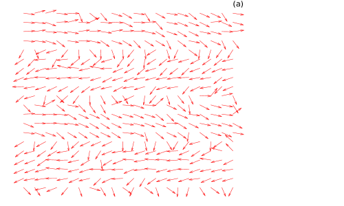
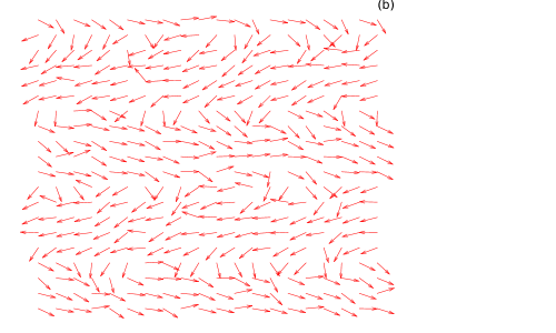
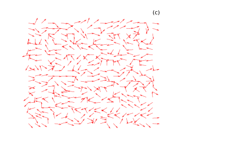
Figure 1: Coherent propagation of driven spin-wave in the XZ plane (Y=10). Wave propagates along the vertical direction. (a) $t=1900$ MCSS and $T=0.4$, (b) $t=1930$ MCSS and $T=0.4$ and (c) $t=2000$ MCSS and $T=2.6$. Here, in all cases, $L=20$, $f=0.01$, $\lambda=10$ and $H=3.0$.

The dynamical responses of the three dimensional XY ferromagnet, driven by linearly polarised propagating magnetic field wave (described above) are studied. Starting from a random initial spin configuration, the system is slowly (in the step of $\Delta T=0.02$ considered here) cooled down to achieve a nonequilibrium steady state. Depending on the values of $T$ and $H$ two distinct dynamical phases are observed. In the low temperature, the coherent motion of bands of spins oriented along a particular directions (on average), is found. One such motion of spin bands are shown in Fig. 1. The spin configuration of a XZ plane (Y=10) is shown here. In the figure, the x-component of the spin lies along the horizontal axis and y-component of the spin lies on the vertical axis. Fig-1(a) and Fig-1(b) show the configurations (for T=0.4 and H=3.0) of spins at two different instants (1900 and 1930 MCSS). The propagating modes of spin bands, along the direction (upward here) of propagation of magnetic wave are clear. This is propagating spin wave mode, observed in XY ferromagnet, driven by linearly polarised (along horizontal direction) propagating (along the Z direction) magnetic field wave. It may be noted here that magnetic wave propagates along the vertical direction and the y-component of spin is shown along the same direction. The lattice has dimensionality three (cubic system) whereas the spin has dimensionality two (XY model). This is the only way one can show the spin configuration of XZ plane in two dimensions. The low temperature spin configurations show that the x-component of spin is nearly zero, on an average. This is due to the response to the linearly (along x-direction) polarised propagating magnetic field wave. However, the y-component (on average) of the spin is nonzero. On the other hand, the high temperature ($T=2.6$) spin configuration (at instant $t=2000$) is completely random (or structureless) and has been shown in Fig-1(c). In this case, both x and y components of the spins are zero separately, on an average.

The propagating mode can also be visualised in another way. The wave is propagating along the z direction. The y component of instantaneous planar magnetisation of any k-th XY plane is calculated as $PMy(k)={{1}\over{L^{2}}}\sum s_{y}$, where the sum is carried over all lattice sites of k-th XY plane. The planar magnetisation (y-component) is plotted against k for two different times and shown in Fig-2. From the figure the propagating mode is evident.

The dynamically stable spin structures, in the low temperature of the system in response to the propagating magnetic field wave are also observed from the study of the statistical distribution of angles (of the spin). The angle $\phi={\rm tan^{-1}}({{s_{y}}\over{s_{x}}})$, where $s_{x}$and $s_{y}$ are the values of x and y component of the spin respectively. The distribution of $\phi$, over all spins ($L^{3}=8000$ here), are calculated at any instant ($t$=2000 here) for two different temperatures. One such distribution (unnormalised), for $T=0.3$ is shown in Fig-3(a). This distribution is trimodal. The three modes occur near $\phi=0$, $\phi\simeq\pi$ (actually slightly above) and $\phi\simeq 2\pi$ (actually slightly below). The distribution vanishes at $\phi={{\pi}\over{2}}$. The distribution gets significantly valuable (nonzero) near $\phi\simeq{{3\pi}\over{2}}$. This distribution of angle $\phi$ assures the existence of a net y component (here negative) with vanishingly small x component of spins. Other kind of distribution of the angles are equally probable (for any other independent sample) which will result the positive net y component. The high temperature ($T=2.6$) structureless spin configuration is justified by the distribution of angle ($\phi$). This is shown in Fig-3(b), where the similar trimodal distribution is observed with almost equal weightage of angles $\phi=0,\pi$ and $2\pi$ leading to vanish the net x component of spin. Similarly, almost equal weightage of angles $\phi={{\pi}\over{2}},{{3\pi}\over{2}}$ compels net y component to vanish.

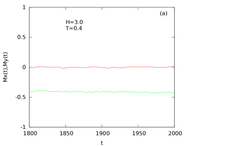
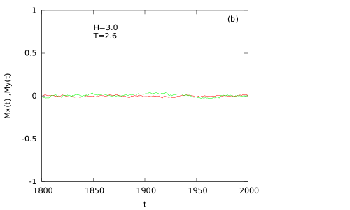
Figure 4: Breaking of the dynamical symmetry in the case of propagating wave. Plots of Mx(t) (red line) and My(t) (green line) as functions of time (t) for different temperatures (a) T=0.4 (symmetry broken phase) and (b) T=2.6 (symmetric phase). In both cases, H=3.0, f=0.01 and $\lambda=10$.

The components (Mx(t) and My(t)) of instantaneous magnetisation are studied as functions of time and shown in Fig. 4. The x-component of instantaneous magnetisation, Mx(t), is close to zero (apart from minor fluctuations) in the low temperature (T=0.4). However, the y-component of this, shows a nonzero value (with some fluctuations). On the other hand, in the high temperature (T=2.6) both vanish (fluctuate around zero). The system undergoes a partial breaking of dynamical symmetry (My(t) only) as it cooled down from high temperature. The existence of the partially dynamic symmetry broken phase, in the low temperature regime, is also evident from the distribution of angles discussed above.

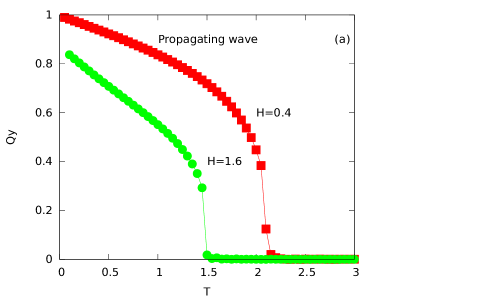
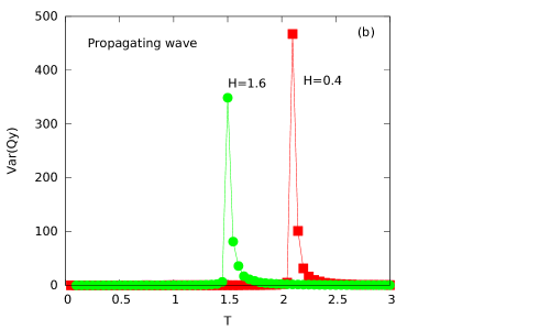
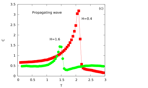
Figure 5: $Qy$, $Var(Qy)$ and $C$ are plotted as functions of the temperature ($T$) for two different values of the amplitude ($H$) of propagating field wave. Here, in all cases, $L=20$, $f=0.01$, $\lambda=10$.

From the usual definition of dynamic order parameter Qx and Qy, it is clear that as the system is cooled down, Qy gets a nonzero value (corresponding to dynamically symmetry broken ordered phase) from Qy=0 (corresponding to dynamically symmetric disordered phase). Needless to say that Qx=0 always. Fig. 5(a) shows the variation of Qy as a function of temperature. There exists a critical temperature, below which Qy$\neq 0$, is so called dynamic transition temperature. This dynamic transition temperature is found to decrease as the amplitude (H) of the propagating field increases. The variance of Qy, i.e., Var(Qy) is found to become sharply peaked at the transition point (Fig. 5(b)). From this diagram, the dynamic transition temperature, is determined and found to decrease as the amplitude of the field (H) increases. Interestingly, the dynamic transition point is also indicated by the temperature, for which the dynamic specific heat C (studied as function of temperature T), gets sharply peaked (Fig. 5(c)).

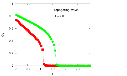
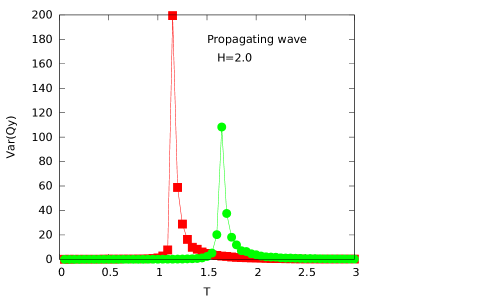
Figure 6: Qy and Var(Qy) are plotted as functions of the temperature ($T$) for two different values of the wavelengths ($\lambda$) of propagating field wave. Red square ($\lambda=20$) and Green bullet ($\lambda=5$). Here, in all cases, $L=20$, $f=0.01$ and $H=2.0$

The dynamic transition temperatures are found to vary with wavelength of the propagating magnetic wave (for fixed value of amplitude). This is shown in Fig. 6. The dynamic order parameter Qy and its variance Var(Qy) are studied as functions of temperature (T) for a two different values ($\lambda=$ 20 and 5) of the wavelength of the propagating magnetic field wave (but with fixed amplitude H=2.0). From the figure it is clear that, the system transits (order - disorder) at lower temperature (fixed $H$) for longer waves of propagating magnetic field wave.

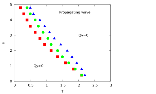
Figure 7: The phase diagrams for propagating wave. Different symbols correspond to the different values of wavelength ($\lambda$). (Red square) $\lambda=20$, (Green bullet) $\lambda=10$ and (Blue triangle) $\lambda=5$.

The dependences of the dynamic transition temperature, on the field amplitude and the wavelength of the propagating magnetic field wave, have been represented in a comprehensive manner in the phase diagram shown in Fig. 7. The phase boundaries are obtained for three different values of the wavelength ($\lambda=$ 20, 10 and 5) of the propagating magnetic wave. The phase boundary is found to shrink (towards low temperature and low field) inward for longer waves of the propagating magnetic field wave.

The detailed finite size analysis, in the system of spins having continuous symmetry, is a huge computational task. One has to determine the critical temperature from the intersection of the fourth order Binder cumulant plotted as functions of temperature for different system sizes. Here, within the limited computational facilities and time, the transition temperatures are calculated crudely from the peak positions of $Var(Qy)$ (studied as function of temperature) for three different values of $L$ ($L=20,30$ and 40). For all values of $L$, the wavelength $\lambda$ was kept fixed ($\lambda=10$). Within the used accuracy ($\Delta T=0.02$ in this simulation), it is observed that the positions of the peaks (for different $L$) remain same (Fig-8). However, the peak height increases as $L$ increases showing the growth of critical correlation (see Fig-2 of ref[3]). This is a peculiar result which shows that (at least from this simulation) the finite size effects do not have any strong dependence on the wavelength $\lambda$. However, further detail investigation is required to have strongly conclusive results.

(b) Standing wave:

Now let us see what happens to the XY ferromagnet if it is driven by standing magnetic field wave. The standing magnetic field wave is extended along the z axis and the polarisation of the field is linear (along the x axis). Here also, two distinct dynamical modes are observed depending upon the values of $T$ and $H$. For a fixed value of $H=3.0$ the low temperature ($T=0.4$) and high temperature ($T=2.6$) spin configurations of any XZ plane (Y=10 here) are shown in Fig-9. In the low temperature, the standing spin wave modes are observed and shown in Fig-9. Unlike the case of propagating spin wave mode, here the spin bands are formed but not changing their positions in time. This indeed reveals the standing spin wave mode. Fig-9(a) and Fig-9(b) shows the spin configurations for two different instants ($t=1900$ and $t=1930$ MCSS). The spin bands are found not to change their positions in time. However, in the high temperature, the structureless or random spin configration was observed (shown in Fig-9(c)).

The standing mode of driven spin wave in XY ferromagnet, can also be visualised in a different way. The y component of planar magnetisation $PMy(k)$ of k-th XY plane are plotted against k and shown in Fig-10 for two different times. From the diagram, it is clear that the profiles ($PMy(k)$ versus $k$) do not change their relative positions in time (unlike the case of propagating mode shown in Fig-2).

The existence of the low temperature ordered (or structured) standing spin wave mode and the high temperature disordered (or structureless) dynamical states can be realised through the statistical distributions of the angles of the spin vectors. The statistical distribution of the angle (of spin vector) $\phi$ is studied and shown in Fig-11. The low temperature unnormalised distribution is shown in Fig-11(a). Here, the distribution is tetramodal (having four maxima). The modes (maxima) of the distributions are found at: $\phi=0$, $\phi\simeq\pi$ (actually slightly above), $\phi\simeq{{3\pi}\over{2}}$ and $\phi\simeq 2\pi$ (actually slightly below). It may be noted that, there was no peak in the distribution of $\phi$, near ${{3\pi}\over{2}}$, in the case of propagating wave (compare with Fig-3(a)). The angle $\phi$ dislikes to accept any value near ${{\pi}\over{2}}$. This peculiar kind of distribution of angle $\phi$ leads to net (nonzero) y component (negative here) of magnetisation. Here also, other kind of distribution of the angles are equally probable (for any other independent sample) which will result the positive net y component. The x component of magnetisation is zero on an average. This is characterised as dynamically ordered phase. On the other hand, the high temperature distribution of angle $\phi$ (shown in Fig-11(b)) is almost symmetric and trimodal (having three maxima of almost equal height) around $\phi=0$, $\phi\simeq\pi$ and $\phi\simeq 2\pi$. Needless to mention that this would lead to a vanishing net y component of magnetisation. The net x component of magnetisation is zero, on an average. This state is characterised as dynamically disordered phase. Like the case of propagating wave (already mentioned above), the ordered phase is a symmetry broken phase and the disordered one is symmetric (in all directions) phase. The partial (in y component only) symmetry broken ordered phase is observed in the case of standing wave.

The dynamical symmetry breaking is clearly visible in the study of the time dependences of the components of magnetisation. The instantaneous components ($Mx(t)$ and $My(t)$) of magnetisation are studied as functions of time and shown in Fig-12. The high temperature ($T=2.6$) study (in Fig-12(a)) shows the existence of a dynamically symmetric phase where both $Mx(t)$ and $My(t)$ varies almost symmetrically around zero line. On the other hand, the dynamical symmetry of the low temperature ($T=0.4$) phase is partially (y component only) broken (Fig-12(b)). In this case, only the y component $My(t)$ varies asymmetrically (about zero line). So, a symmetry breaking dynamic (or nonequilibrium) transition is expected in the driven (by standing magnetic wave) XY ferromagnet. It may be noted that in both phases, the time average x component of magnetisation over the full cycle of the standing magnetic wave is zero.

To study the symmetry breaking dynamic phase transition in driven XY ferromagnet, the temperature dependences of $Qy$, $Var(Qy)$ and $C$ are studied and shown in Fig-13. For a fixed value of $H$, the $Qy$ takes a nonzero value near a transition temperature as the system is cooled down from a high temperature. This transition temperature is found to decrease as the value of $H$ is increased. This is shown in Fig-13(a). The $Var(Qy)$ and $C$ show sharp peaks near the transition temperatures. They are shown in Fig-13(b) and Fig-13(c). The peaks determine the transition temperatures. From all these studies it is clear that the transitions occur at lower temperatures for higher values of the field amplitudes ($H$).

Obtaining the values of dynamic transition temperatures from the peak positions of $Var(Qy)$ and $C$ for different values of the amplitudes ($H$) the comprehensive phase diagrams are obtained and shown in Fig-14. Here also, the phase boundaries are drawn for three different ($\lambda=$ 20, 10 and 5) values of the wavelength of standing magnetic field wave. Unlike the case of propagating wave, the phase boundaries do not show any systematic variation with the wavelength of the standing magnetic wave, in this simulational study.

Here also, the transition temperatures are calculated from the peak position of $Var(Qy)$ (studied as function of temperature) for three different values of $L$ ($L=20,30$ and 40). Within the used accuracy ($\Delta T=0.02$ in this simulation), it is observed that the positions of the peaks (for different $L$) remain same (Fig-15). In this case also, the peak height is observed to increase as $L$ increases showing the similar growth of critical correlation.

IV. Summary

The dynamical (or nonequilibrium) responses of classical XY ferromagnet driven by linearly polarised propagating and standing magnetic field wave have been investigated by Monte Carlo simulation using Metropolis algorithm in three dimensions. The system is a simple cube of length (of each side) $L$ having periodic boundary conditions in all three directions.

In the case of propagating magnetic field wave, with specified amplitude, frequency and the wavelength, the system shows various dynamical responses depending on the temperature. In the low temperature, the nonequilibrium steady state is dynamically structured. The coherent motion of the spin bands (or spin wave) was observed along the direction of the propagating magnetic field wave. In this phase, a nonzero net y component of magnetisation was observed with vanishing average x component. The y component varies asymmetrically (about zero) with time. The time averaged y component of the magnetisation over the full cycle of the propagating field wave (i.e., the y component of dynamic order parameter) is nonzero. On the other hand, the high temperature, dynamical state is structureless or randomly oriented. As a result, both x and y components of the time averaged magnetisations, over the full cycle of the propagating magnetic wave, vanish. The x and y components of the magnetisation, vary symmetrically (about zero) with time. A partially (in y component only) symmetry breaking dynamic nonequilibrium phase transition was observed at any finite temperature. This symmetry breaking was observed independently from the distribution of the angles of the spin vectors. This transition temperature was found from the temperature dependences of dynamic order parameter, its variance and the dynamic specific heat. The dynamic transition was found to occur at lower temperature with higher values of the amplitude of the propagating field. A comprehensive nonequilibrium phase boundary was drawn in the plane formed by the temperature and amplitude of the propagating field wave. The phase boundary shrinks towards the low temperature region for longer wavelength of the propagating magnetic field wave. A remarkable and interesting difference in the nonequilibrium phases, with that observed in the discrete spin models (Ising, Blume-Capel etc) [9, 12], is the absence of any pinned (or spin frozen) phase in the low temperaure. The continuous spin models (like classical XY etc.) does not require any threshold field to change the state of individual spin which is essential for discrete spin systems. The phase boundaries were observed to approach the equilibrium critical temperature (around 2.20$J/k$) [29] for vanishingly small value of the field amplitude.

In the case of standing magnetic field wave, the low temperature nonequilibrium phase is a standing spin wave. Here also the symmetry breaking nonequilibrium phase transition was observed. The dynamic phase boundary was drawn. Unlike the case of propagating magnetic wave, here the phase boundary does not show any significant dependence on the wavelength of the standing magnetic field wave. However, like the case of propagating wave, the dynamic critical temperature was observed to approach the equilibrium value (approximately 2.20$J/k$) [29], as the value of the field amplitude approaches zero.

Although the theoretical understanding of nonequilibrium phase transition is not yet well developed, one may try to realise the effects as follows: The three dimensional XY ferromagnet has an equilibrium critical temperature[29] where the time scale (relaxation time) diverges. Now consider, this system is being driven by propagating magnetic field wave, which keeps the system away from the equilibrium. This propagating magnetic field wave has a characteristic time (time period) and a characteristic length (the wavelength). The nonequilibrium phase transition is the outcome of the competition between the time scale of the driving field and the intrinsic time scale (relaxation time) of the system. As the system is cooled from high temperature (having random spin configuration) the intrinsic time scale of the system increases. As a result, system gradually fails to follow the driving field. Due to the relaxational delay, a phase lag, between the response and the time dependent perturbation, developes. This gives rise to dynamical ordering of the system. In this case, since the polarisation of the field is along the X direction, the spin vector fails to follow the field. Consequently, the Y component has a net average value, while the net X component becomes zero. And for higher values of the field, the transition would occur at lower temperatures.

The phase boundary (particularly, in the case of propagating wave) was observed to shrink (towards lower values of field strength and temperature). This may be realised qualitatively as follows: The wavelength measures the extension of the exposed zone for the spin flips. As this area increases the lower value of temperature and field strength would be adequate to set the dynamical order in the system. However, this picture is incapable of explaining the complicated variation of the phase boundary as function of the wavelength in the case of standing wave. Further extensive investigations are required for clear understanding of this behaviour of the phase boundary.

This study is an appeal to the experimentalists to see the effect of spin dynamics in the ferromagnetic polycrystals like ${\rm Fe[Se_{2}CN(C_{2}H_{5})_{2}]_{2}Cl}$ and ${\rm Zn[S_{2}CN(C_{2}H_{5})_{2}]_{2}}$ which can be modelled by site diluted classical XY system [27] with superexchange interactions. In the field of spintronics [28] it is also important to know the response and thermodynamical behaviours of ferromagnetic systems driven by intense optical perturbations.

References

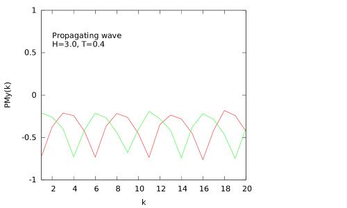
Figure 2: The y-component of planar magnetisation PMy(k) plotted against k (k-th XY plane). Different colors represent different time (a) t=1900 MCSS (red line) and (b) t=1930 MCSS (green line). The propagating wave moves along z direction.

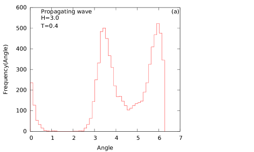
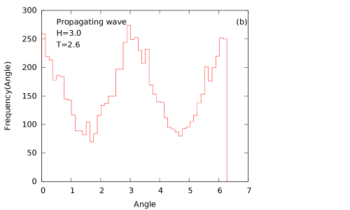
Figure 3: Unnormalized distribution of angles of the spin vectors for propagating waves. (a) $t=2000$ MCSS and $T=0.4$, (b) $t=2000$ MCSS and $T=2.6$. Here, in all cases, $L=20$, $f=0.01$, $\lambda=10$ and $H=3.0$.

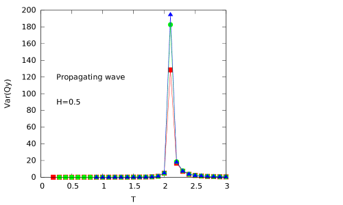
Figure 8: The size dependence of the transition temperature in the case of propagating wave. Different symbols correspond to the different values of system size ($L$). (Red square) $L=20$, (Green bullet) $L=30$ and (Blue triangle) $L=40$. The wavelength of the propagating wave $\lambda=10$ lattice unit in all three cases.

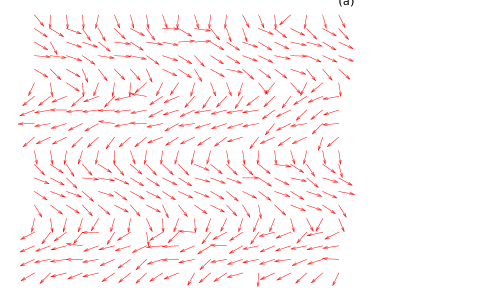
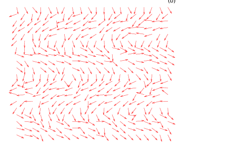
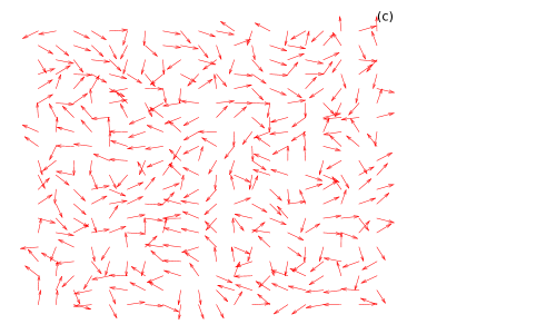
Figure 9: Standing mode of driven spin-wave in the XZ plane (Y=10). (a) $t=1900$ MCSS and $T=0.4$, (b) $t=1930$ MCSS and $T=0.4$ and (c) $t=2000$ MCSS and $T=2.6$. Here, in all cases, $L=20$, $f=0.01$, $\lambda=10$ and $H=3.0$.

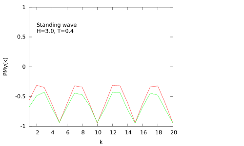
Figure 10: The y-component of planar magnetisation PMy(k) plotted against k (k-th XY plane). Different colors represent different time (a) t=1900 MCSS (red line) and (b) t=1930 MCSS (green line). The standing wave extends along z direction.

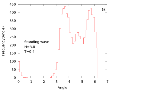
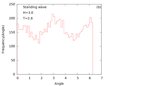
Figure 11: Unnormalized distribution of angles of the spin vectors for standing magnetic waves. (a) $t=2000$ MCSS and $T=0.4$, (b) $t=2000$ MCSS and $T=2.6$. Here, in all cases, $L=20$, $f=0.01$, $\lambda=10$ and $H=3.0$.

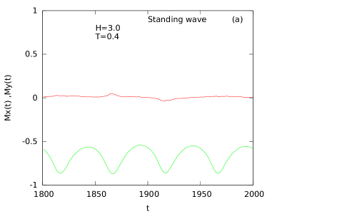
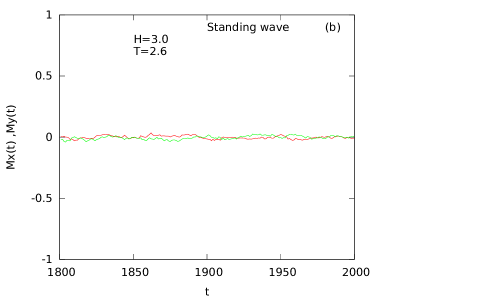
Figure 12: Breaking of the dynamical symmetry in the case of standing wave. Plots of Mx(t) (red line) and My(t) (green line) as functions of time (t) for different temperatures (a) T=0.4 (symmetry broken phase) and (b) T=2.6 (symmetric phase). In both cases, H=3.0, f=0.01 and $\lambda=10$.

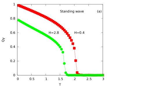
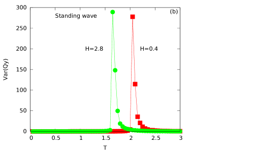
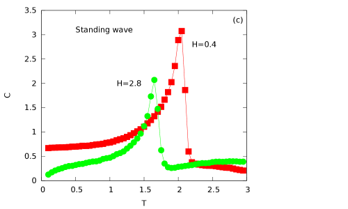
Figure 13: Qy, Var(Qy) and C are plotted as functions of the temperature ($T$) for two different values of the amplitude ($H$) of standing magnetic field wave. Here, in all cases, $L=20$, $f=0.01$, $\lambda=10$.

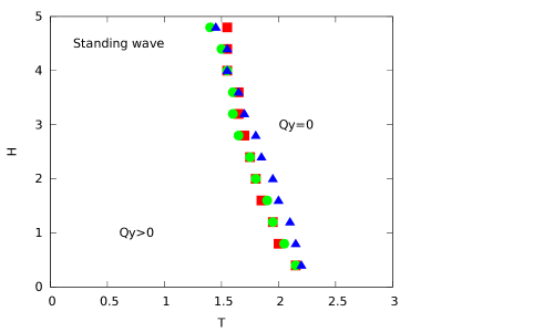
Figure 14: The phase diagrams for standing wave. Different symbols correspond to the different values of wavelength ($\lambda$). (Red square) $\lambda=20$, (Green bullet) $\lambda=10$ and (Blue triangle) $\lambda=5$.

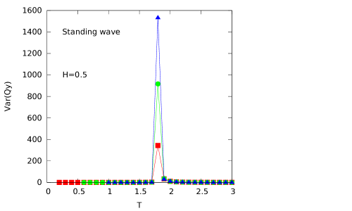
Figure 15: The size dependence of the transition temperature in the case of standing wave. Different symbols correspond to the different values of system size ($L$). (Red square) $L=20$, (Green bullet) $L=30$ and (Blue triangle) $L=40$. The wavelength of the standing wave $\lambda=10$ lattice unit, in all three cases.

References

- [1] Chakrabarti BK and Acharyya M. Dynamic transitions and hysteresis. Rev. Mod. Phys. 1999; 71:847
- [2] Acharyya M. Nonequilibrium phase transitions in model ferromagnets: A review. Int. J. Mod. Phys. C, 2005;16:1631
- [3] Sides R, Rikvold PA and Novotny MA. Kinetic Ising model in an oscillating field: Finite size scaling at the dynamic phase transition. Phys. Rev. Lett. 1998;81:834
- [4] Park H and Pleimling M. Surface criticality at a dynamic phase transition. Phys. Rev. Lett. 2012; 109 : 175703; Erratum, Phys. Rev. Lett. 2013; 110: 239903
- [5] Reigo P, Vavassori P and Berger A. Metamagnetic anomalies near dynamic phase transition. Phys. Rev. Lett. 2017; 118: 117202
- [6] Buendia GM and Rikvold PA. Fluctuations in a model ferromagnetic film driven by a slowly oscillating field with a constant bias. Phys. Rev. B. 2017; 96: 134306
- [7] Berger A, Idigoras O, and Vavassori P. Transient behaviour of the dynamically ordered phase in uniaxial cobalt film. Phys. Rev. Lett. 2013; 111: 190602
- [8] Acharyya M. Nonequilibrium phase transition in the kinetic Ising model driven by propagating magnetic field wave. Physica Scripta. 2011; 84: 035009
- [9] Halder A and Acharyya M. Standing magnetic wave on Ising ferromagnet: Nonequilibrium phase transition. J. Magn. Magn. Mater. 2016; 420: 290
- [10] Acharyya M. Standing spin wave mode in RFIM: Patterns and athermal nonequilibrium phases J. Magn. Magn. Mater. 2015; 394: 410
- [11] Acharyya M. Dynamic symmetry breaking breathing and spreading transitions in ferromagnetic film irradiated by spherical electromagnetic wave. J. Magn. Magn. Mater. 2014; 354: 349
- [12] Acharyya M and Halder A. Blume-Capel ferromagnet driven by propagating and standing magnetic field wave: Dynamical modes and nonequilibrium phase transition. J. Magn. Magn. Mater. 2017; 426: 53
- [13] Acharyya M. Ising metamagnet driven by propagating magnetic field wave: Nonequilibrium phases and transitions. J. Magn. Magn. Mater. 2015; 382: 206
- [14] Kosterlitz JM and Thouless DJ. Ordering, metastability and phase transitions in twi dimensional systems. Journal of Physics C: Solid State Physics 1973; 6: 1181
- [15] Evertz EG and Landau DP. Critical dynamics in the two-dimensional classical XY model: A spin dynamics study. Phys. Rev. B. 1996; 54: 12302
- [16] Landau DP, Pandey R and Binder K. Monte Carlo study of the surface critical behaviour in the XY model. Phys. Rev. B. 1989; 39: 12302
- [17] Rastelli E, Regina S and Tassi A. Monte Carlo study of the planar rotator model with symmetry breaking fields. Phys. Rev. B. 2004; 69: 174407
- [18] Olsson P. Vortex glass transition in disordered three dimensional XY models: Simulations for several different sets of parameters. Phys. Rev. B. 2005; 72: 144525
- [19] Guimaraes M, Costa BV, Pires AST and Souza A. Phase diagram of the 3D quantum anisotropic XY model- A quantum Monte Carlo calculation. J. Magn. Magn. Mater. 2013; 332: 103
- [20] Lapa RS and Pires AST. Critical properties of the frustrated quasi two dimensitional XY like antiferromagnets. J. Magn. Magn. Mater. 2013; 327: 1
- [21] Ciftza O and Prenga D. Magnetic properties of a classical XY spin dimer in a ”planar” magnetic field. J. Magn. Magn. Mater. 2016; 416: 220
- [22] Berthier L, Holdsworth PCW and Sellitto M. Nonequilibrium critical dynamics of the two dimensional XY model. J. Phys. A: Math. Gen. 2001; 34: 1805
- [23] Ajisaka S, Barra F and Zunkovic B. Nonequilibrium quantum phase transition in the XY model: Comparison of unitary time evolution and reduced density operator approaches. New J. Phys. 2014; 16: 033028
- [24] Teles TN, Benetti FP, Parkter R and Levin Y. Nonequilibrium phase transition in systems with long range interactions. Phys. Rev. Lett. 2012; 109: 230601
- [25] Yasui T, Tutu H, Yamamoto M and Fujisaka H. Dynamic phase transition in the anisotropic XY spin system in an oscillating magnetic field. Phys. Rev. E. 2002; 66: 036123
- [26] Metropolis N, Rosenbluth AW, Rosenbluth MN and Teller AH. Equation of state calculations by fast computing machines. J. Chem. Phys. 1953; 21: 1087
- [27] Santos-Filho JB and Plascak JA. Monte Carlo study of the site diluted 3D XY model with superexchange interaction: Application to diluted magnets. Phys. Lett. A. 2015; 379: 3119
- [28] Bader S and Parkin SSP. Spintronics. Ann. Rev. Cond. Mat. Phys. 2010; 1: 71-88
- [29] Hasenbusch M. A Monte Carlo study of the three dimensional XY universality class: Universal amplitude ratios. J. Stat. Mech. 2008; 12: P12006