Deep laser cooling in optical trap: two-level quantum model

Abstract

We study laser cooling of ²⁴Mg atoms in dipole optical trap with pumping field resonant to narrow $(3s3s)\,^{1}S_{0}\rightarrow\,(3s3p)\,^{3}P_{1}$ ($\lambda=457$ nm) optical transition. For description of laser cooling of atoms in the optical trap with taking into account quantum recoil effects we consider two quantum models. The first one is based on direct numerical solution of quantum kinetic equation for atom density matrix and the second one is simplified model based on decomposition of atom density matrix over vibration states in the dipole trap. We search pumping field intensity and detuning for minimum cooling energy and fast laser cooling.

Pacs 32.80.Pj, 42.50.Vk, 37.10.Jk,37.10.De

1 Introduction

Nowadays deep laser cooling of neutral atoms is routinely used for broad range of modern quantum physics researches including metrology, atom optics, and quantum degeneracy studies. The well-known techniques for laser cooling below the Doppler limit, like sub-Doppler polarization gradient cooling [1], velocity selective coherent population trapping [2, 3] or Raman cooling [4, 5] are restricted to atoms with degenerated over angular momentum energy levels or hyperfine structure. However, for atoms with single ground state ²⁴Mg, ⁴⁰Ca, ⁸⁸Sr, ¹⁷⁴Yb are of interest for developing optical time standard these techniques can not be applied directly. For example, for ²⁴Mg atoms with the ground state ${}^{1}S_{0}$ the Doppler cooling temperature ($k_{B}T_{D}\approx\hbar\gamma/2$) can be reached on closed singlet transition ${}^{1}S_{0}\rightarrow\,^{1}P_{1}$ ($\lambda=285.3$ nm). For lower temperature additional cooling on ${}^{3}P_{2}\rightarrow\,^{3}D_{3}$ optical transition with degenerated over angular momentum energy levels can be applied [6, 7]. However, the experimental realization of laser cooling on ${}^{3}P_{2}\rightarrow\,^{3}D_{3}$ optical transition does not result significant progress. The atoms were cooled to temperature $T\approx 1\,mK$ is about Doppler limit only [7]. The quantum simulation of laser cooling are also shows the limitation of cooling temperature to about Doppler limit in conventional MOT, formed by laser waves with circular polarization [8].

An alternative way of deep laser cooling of these elements is to use narrow lines and “quenching” techniques of narrow-line laser cooling [9, 10, 11] successfully applied for ⁴⁰Ca atoms but, to our knowledge, still do not show significant progress for ²⁴Mg atoms.

Recently, laser-driven Sisyphus-cooling scheme was proposed for cooling atoms in optical dipole trap [12]. This scheme utilize the difference in trap-induced ac Stark shift for ground and exited levels of atom coupled by resonant laser light. The laser cooling scheme has clear semiclassical interpretation: been excited by resonant laser light on the bottom of shallow optical potential related to the ground state an atom moves further in steepest potential related to excited state. Spontaneous emission returns it back to the shallow potential in the ground state. The loosing a portion of energy in each act of this process results to atom cooling after several cycles due to “Sisyphus effect” [12]. This semiclassical model was applied for description of laser cooling of Yb and Sr in optical dipole trap.

Figure 1: Relevant energy levels for optical quenching and cooling of ²⁴Mg.

In the following paper we study application of this cooling scheme to ²⁴Mg atom on narrow $(3s3s)\,^{1}S_{0}\rightarrow\,(3s3p)\,^{3}P_{1}$ ($\lambda_{1}=457$ nm, $\gamma_{1}=196$ s^-1) optical transition. Additional light field resonant to $(3s3p)\,^{3}P_{1}\rightarrow\,(3s4s)\,^{1}S_{0}$ optical transition ($\lambda_{2}=462$ nm, $\gamma_{21}=109$ s^-1 and $\gamma_{23}=2.1\cdot 10^{7}$ s^-1) is applied for optical quenching (see Fig.1), i.e. increasing the effective linewidth of optical transition [11]. We find the semiclassical description of laser cooling of Mg atom with narrow optical transition can’t be used here. For description of laser cooling we use quantum approaches that allow to take into account optical pumping and photon recoil effects in laser cooling process. In the paper we point our attention to minimum laser cooling temperature for described scheme and cooling time as well.

Figure 2: Ac Shtark shift and vibration energy levels for ground ${}^{1}S_{0}$ (a) and excited ${}^{3}P_{1}$ (b) states of ²⁴Mg atoms in dipole optical trap with $\lambda_{D}=1064$nm.

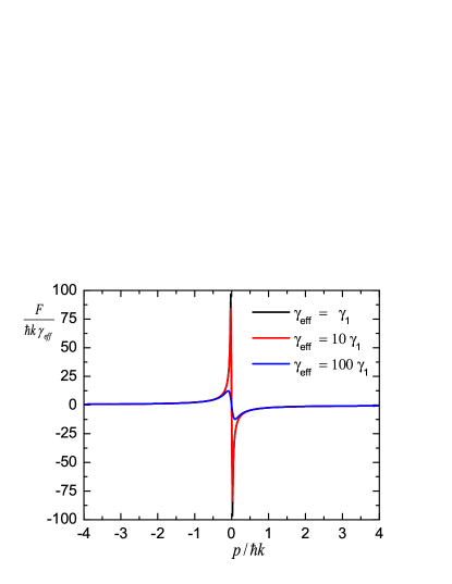
Figure 3: Force on moving ²⁴Mg atoms in the dipole trap ($U_{g}=200\,\mu K$, $U_{e}=292\,\mu K$) for different $\gamma_{eff}$. Here $\delta_{1}=0$, Rabi of pumping field $\Omega_{1}/\gamma_{1}=20000$ ($I\simeq 34$ $W/cm^{2}$).

2 Description of the model

We consider the motion of ²⁴Mg atom in the dipole optical trap with $\lambda_{D}=1064\,nm$ that provide higher polarizability of atom in the excited state $(3s3p)\,^{3}P_{1}$ than in the ground state $(3s3s)\,^{1}S_{0}$. In the following paper we restrict our consideration by two-level model assuming the quench field results to increasing effective linewidth of optical transition to $\gamma_{eff}$ [11]:

$$\gamma_{eff}=\gamma_{1}+\gamma_{2}\frac{\Omega_{2}^{2}}{\gamma_{2}^{2}+4\,\delta_{2}^{2}}\,,$$ (1)

where $\Omega_{2}$ is Rabi and $\delta_{2}$ is detuning of quench field. Thus, for example, to get $\gamma_{eff}=100\gamma_{1}$ at $\delta_{2}=0$ one have to apply the quench field intensity $I_{q}\approx 1.6\,W/cm^{2}$. The simulated polarizability difference for the optical dipole trap wavelength is about $\alpha_{e}/\alpha_{g}=1.46$. In the trap (fig.2) the quantum nature of atomic motion becomes essential. For considered optical trap depth of the ground state $U_{g}=200\,\mu K$ with vibration energy separation of the lowest states are $\hbar\omega_{g}\approx 16.6\,\mu K$. The excited state optical potential depth $U_{e}=292\,\mu K$ and the lowest states separation are $\hbar\omega_{e}\approx 20.1\,\mu K$. The large energy levels separation require quantum model for description of laser cooling dynamics of atoms in the trap. Really, the semiclassical models can’t be applied here because of the velocity range of the semiclassical damping force on Mg atoms has sharp variation in momentum space $\Delta p\ll\hbar k$ (see figure 3). As well the semiclassical parameter $\varepsilon_{R}=\hbar k^{2}/(2M\gamma)\gg 1$ is not small, that also contradicts requirements for semiclassical approach [1, 13, 14].

For description of laser cooling of Mg in the optical trap we consider two quantum approaches. The first one is based on decomposition of atom density matrix on optical potential vibration level states. Restricting by limited number of lowest vibration states we simulate the stationary distribution over the vibration levels in the trap, as well as the laser cooling dynamics to steady state distribution. This approach is similar to method was described in [15]. However, in our model we also take into account the optical coherence of different vibration states.

The second method we consider is based on direct numerical solution of quantum equation for atom density matrix that allows to take into account not only the fixed number of the lowest vibration level states but whole density matrix of atoms, which also include tunneling effects and above barrier motion. However, in this method, due to the high complicity of the problem we omit the recoil effects from the pumping field that is equivalent to orthogonal orientation of wave vectors of pumping and optical trap light waves in one dimensional model.

2.1 Two-level model: exact numerical solution of quantum density matrix equation

We consider the motion of Mg atom in the optical dipole trap is standing light wave propagating along $z$ direction with linear polarization along $x$. The pumping light field also linear polarized along $x$ with wavevector along $z$ or $y$. The quantum equation for atom density matrix describes evolution of internal and external states of atoms

$$\frac{\partial}{\partial t}{\hat{\rho}}=-\frac{i}{\hbar}\left[{\hat{H}}_{0}+{\hat{V}}_{ed},{\hat{\rho}}\right]+{\hat{\Gamma}}\left\{{\hat{\rho}}\right\}$$ (2)

with ${\hat{H}}_{0}$ is Hamiltonian, ${\hat{V}}_{ed}$ describes interaction with pumping field and ${\hat{\Gamma}}\left\{{\hat{\rho}}\right\}$ describes relaxation of density matrix due to spontaneous decay.

As was mentioned above, we restrict our consideration by effective two-level model with $(3s3s)\,^{1}S_{0}$ is the ground (g) and $(3s3p)\,^{3}P_{1}$ is excited state (e), assuming the influence of the quench field $\Omega_{2}$ results to adjustable linewidth by modification of decay rate from $\gamma_{1}$ to $\gamma_{eff}$ only, as described in [11]. Further in the paper we omit parameters indexes $\Omega_{1}$, $\delta_{1}$ and $\gamma_{1}$ by writing $\Omega$, $\delta$ and $\gamma$ instead. The Hamiltonian of atom in the trap has the form:

$${\hat{H}}_{0}=\frac{{\hat{p}}^{2}}{2M}+\hbar\omega_{g}(z)|g\rangle\langle g|+\hbar[\omega_{e}(z)+\omega_{0}]|e\rangle\langle e|$$ (3)

with optical potentials in the ground $\hbar\omega_{g}(z)=U_{g}\cos^{2}(kz)$ and $\hbar\omega_{e}(z)=U_{e}\cos^{2}(kz)$ in excited states ($\hbar\omega_{0}=E_{e}-E_{g}$ is energy difference of unperturbed ground and excited states). The wavevector $k=2\pi/\lambda_{D}$ is defined by the dipole trap. Applying rotating wave approximation the equation for atom density matrix components in coordinate representation ${\hat{\rho}}(z_{1},z_{2})$ takes the followign form:

$$\left(\frac{\partial}{\partial t}-\frac{i\hbar}{M}\frac{\partial}{\partial q}\frac{\partial}{\partial z}\right)\rho^{ee} = -\gamma_{eff}\,\rho^{ee}+i\frac{U_{e}}{\hbar}\sin(2kz)\sin(kq)\rho^{ee}-\frac{i}{\hbar}\left[{\hat{V}}\rho^{ge}-\rho^{eg}{\hat{V}}^{\dagger}\right]$$

$$\left(\frac{\partial}{\partial t}-\frac{i\hbar}{M}\frac{\partial}{\partial q}\frac{\partial}{\partial z}\right)\rho^{gg} = {\hat{\gamma}}\{\rho^{ee}\}+i\frac{U_{g}}{\hbar}\sin(2kz)\sin(kq)\rho^{gg}-\frac{i}{\hbar}\left[{\hat{V}}^{\dagger}\rho^{eg}-\rho^{ge}{\hat{V}}\right]$$

$$\left(\frac{\partial}{\partial t}-\frac{i\hbar}{M}\frac{\partial}{\partial q}\frac{\partial}{\partial z}\right)\rho^{eg} + \left(\frac{\gamma_{eff}}{2}-i\tilde{\delta}(z,q)\right)\rho^{eg}=-\frac{i}{\hbar}\left[{\hat{V}}\rho^{gg}-\rho^{ee}{\hat{V}}\right]$$

$$\left(\frac{\partial}{\partial t}-\frac{i\hbar}{M}\frac{\partial}{\partial q}\frac{\partial}{\partial z}\right)\rho^{ee} + \left(\frac{\gamma_{eff}}{2}+i\tilde{\delta}(z,-q)\right)\rho^{ge}=-\frac{i}{\hbar}\left[{\hat{V}}^{\dagger}\rho^{ee}-\rho^{gg}{\hat{V}}^{\dagger}\right]\,,$$ (4)

with $z=(z_{1}+z_{2})/2$, $q=z_{1}-z_{2}$, and the function $\tilde{\delta}(z,q)$:

$$\tilde{\delta}(z,q)=\delta-(U_{e}-U_{g})\frac{1+\cos(2kz)\cos(kq)}{2\hbar}+(U_{e}+U_{g})\frac{\sin(2kz)\sin(kq)}{2\hbar}.$$

The spontaneous income part to the ground state ${\hat{\gamma}}$ in coordinate representation for two-level model has simple form :

$${\hat{\gamma}}\{\rho^{ee}\} = {\tilde{\gamma}}(q)\rho^{ee}$$

$${\tilde{\gamma}}(q) = 3\,\gamma_{eff}\left(\frac{\sin(k_{1}q)}{(k_{1}q)^{3}}-\frac{\cos(k_{1}q)}{(k_{1}q)^{2}}\right)$$ (5)

with $k_{1}=2\pi/\lambda$ is wavevector of emitted photon. The pumping field induces transitions between the ground and excited states. This part is described in (2.1) by operator

$${\hat{V}}=\Omega/2\,\exp(ik_{1}z\cos(\theta))$$ (6)

with $\Omega$ is Rabi frequency of pumping field and $\theta$ is angle between the axis $z$ and pumping wave propagation direction. For the case of orthogonal orientation of the pumping wave propagation to the dipole trap $\theta=\pi/2$ the equation for density matrix (2.1) can be solved numerically by the method suggested in [16, 17]. It should be noted the considered method allows to get steady state solution for density matrix with taking into account quantum recoil effects as for atoms in the trap as for nontrapped atoms.

Figure 4: Spatial (a) and momentum (b) distribution of ²⁴Mg atoms in optical dipole trap ($U_{g}=200\,\mu K$, $U_{e}=292\,\mu K$) for orthogonal orientation of pumping wave and dipole trap ($\theta=\pi/2$) and pumping field intensity $I\simeq 34$ $W/cm^{2}$ ($\Omega/\gamma=20000$) and different detunings.

The figure 4 shows spatial and momentum distribution of Mg atoms in the optical dipole trap for orthogonal orientation of pumping wave ($\theta=\pi/2$), for pumping field intensity $I\simeq 34$ $W/cm^{2}$ ($\Omega/\gamma=20000$) and different detunings.

The obtained numerical solution for steady state density matrix ${\hat{\rho}}(z_{1},z_{2})$ contains whole information on internal and external states of atoms in the trap. In particular one can extract the population of vibration levels in the ground and excited states:

$$\rho^{ee}_{n} = \int\psi^{*(e)}_{n}(z_{1})\rho^{ee}(z_{1},z_{2})\psi^{(e)}_{n}(z_{2})dz_{1}dz_{2}\,,$$

$$\rho^{gg}_{n} = \int\psi^{*(g)}_{n}(z_{1})\rho^{gg}(z_{1},z_{2})\psi^{(g)}_{n}(z_{2})dz_{1}dz_{2}$$ (7)

where $\psi^{(e,g)}_{n}(z)$ are n-th vibration level eigenfunctions. The distribution of vibration levels population in the ground and excited states for parameters of figure 4 are shown on figure 5.

Figure 5: Vibration energy levels population distribution in the ground (a) and excited (b) states of ²⁴Mg atoms in the dipole trap ($U_{g}=200\,\mu K$, $U_{e}=292\,\mu K$) for orthogonal orientation of pumping wave and dipole trap ($\theta=\pi/2$). Pumping field intensity $I\simeq 34$ $W/cm^{2}$ ($\Omega/\gamma=20000$).

The energy of cooled atoms can be found by different way. First of all one can use the relation for the temperature of cooled atoms in the well known form

$$k_{B}T=<p^{2}>/M\,,$$ (8)

with $<p^{2}>=Tr\{{\hat{p}}^{2}\,{\hat{\rho}}\}$. This relation neglects the atom localization effects in the optical potential. The most accurate relation for energy is expressed by the following averaging:

$$E=Tr\left\{\left(\frac{{\hat{p}}^{2}}{2M}\,+\hbar\omega_{e}(z)\right){\hat{\rho}^{(ee)}}\right\}+Tr\left\{\left(\frac{{\hat{p}}^{2}}{2M}\,+\hbar\omega_{g}(z)\right){\hat{\rho}^{(gg)}}\right\}\,.$$ (9)

As an alternative way one can find the average energy over the vibration states

$$E=\sum_{n}E^{(e)}_{n}\,\rho^{(ee)}_{n}+E^{(g)}_{n}\,\rho^{(gg)}_{n}.$$ (10)

For considered parameters all above definitions give very close values that denotes the main contribution to energy are given by atoms on the lowest vibration energy levels in the region where the optical potential has close to parabola shape. The energy of Mg atoms for different detuning is shown on figure 6. The total population of excited vibration level states here do not exceed $2\%$ and are not shown on figure 6(b). In the region of detuning $\delta>-6000\gamma$ we find inversion of the lowest vibration levels population resulting to energy growth. For the higher intensity of pumping field this effect is also exists and moves to larger detuning area. The energy of atoms as function of pumping field intensity for different detunings is shown on figure (7).

Figure 6: The energy (a) of cooled ²⁴Mg atoms in the dipole trap and population of the lowest vibration levels (b) as function of pumping field detuning for $I\simeq 0.34$ $W/cm^{2}$ ($\Omega/\gamma=2000$) obtained by direct numerical solution of eq.(2.1). ($\theta=\pi/2$)

Figure 7: The energy of cooled ²⁴Mg atoms in the dipole trap ($\theta=\pi/2$) obtained by direct numerical solution of eq.(2.1) as function of pumping field intensity for different detunings.

2.2 Decomposition on vibration states model

As we see from the simulations above based on numerical solution of basic equation for atomic density matrix (2.1) for the considered parameters Mg atoms can be cooled and well localized in the dipole trap. Thus for description of laser coolling and laser cooling time we can also apply an alternative approach based on decomposition of atom density matrix over vibration level states.

$${\hat{\rho}}=\left(\begin{array}[]{cc}\left[\begin{array}[]{ccc}{\rho}^{ee}_{00}&{\rho}^{ee}_{01}&...\\ {\rho}^{ee}_{10}&{\rho}^{ee}_{11}&...\\ ...&...&{\rho}^{ee}_{nm}\\ \end{array}\right]&\left[\begin{array}[]{ccc}{\rho}^{eg}_{00}&{\rho}^{eg}_{01}&...\\ {\rho}^{eg}_{10}&{\rho}^{eg}_{11}&...\\ ...&...&{\rho}^{eg}_{nm}\\ \end{array}\right]\\ \left[\begin{array}[]{ccc}{\rho}^{ge}_{00}&{\rho}^{ge}_{01}&...\\ {\rho}^{ge}_{10}&{\rho}^{ge}_{11}&...\\ ...&...&{\rho}^{ge}_{nm}\\ \end{array}\right]&\left[\begin{array}[]{ccc}{\rho}^{gg}_{00}&{\rho}^{gg}_{01}&...\\ {\rho}^{gg}_{10}&{\rho}^{gg}_{11}&...\\ ...&...&{\rho}^{gg}_{nm}\\ \end{array}\right]\\ \end{array}\right)$$ (11)

The equation for these components takes the form:

$$\frac{\partial}{\partial t}{\hat{\rho}}=-\frac{i}{\hbar}\left[{\hat{H}}_{0}+{\hat{W}},{\hat{\rho}}\right]+\Gamma\{{\hat{\rho}}\}$$ (12)

with Hamiltonian

$${\hat{H}}_{0}=\left(\begin{array}[]{cc}\left[\begin{array}[]{ccc}E^{(e)}_{0}-\hbar\delta&0&...\\ 0&E^{(e)}_{1}-\hbar\delta&...\\ ...&...&E^{(e)}_{n}-\hbar\delta\\ \end{array}\right]&\left[\begin{array}[]{ccc}0&0&...\\ 0&0&...\\ ...&...&0\\ \end{array}\right]\\ \left[\begin{array}[]{ccc}0&0&...\\ 0&0&...\\ ...&...&0\\ \end{array}\right]&\left[\begin{array}[]{ccc}E^{(g)}_{0}&0&...\\ 0&E^{(g)}_{1}&...\\ ...&...&E^{(g)}_{n}\\ \end{array}\right]\\ \end{array}\right)$$ (13)

where $E^{(e)}_{n}$ and $E^{(g)}_{n}$ are the vibration levels energy of the excited and the ground states. The pumping light field to atom interaction part has nondiagonal block elements only:

$$W^{eg}_{nm}=\langle e,n|{\hat{V}}|g,m\rangle=\int\psi^{*(e)}_{n}(z){\hat{V}}\psi^{(g)}_{m}(z)dz\,.$$ (14)

with ${\hat{V}}$ is defined in (6). The spontaneous relaxation part $\Gamma\{{\hat{\rho}}\}$ has a standard form

$$\Gamma\{{\hat{\rho}}\}=-\frac{\gamma_{eff}}{2}\left\{|e,n\rangle\langle e,n|,{\hat{\rho}}\right\}+{\hat{\gamma}}\left\{{\hat{\rho}}\right\}$$ (15)

with ${\hat{\gamma}}\left\{{\hat{\rho}}\right\}$ describes income to the ground vibration states has the following matrix elements:

$${\hat{\gamma}}\left\{{\hat{\rho}}\right\}_{nm} = \sum_{\nu\mu}\Gamma^{\nu\mu}_{nm}{\rho}^{ee}_{\nu\mu}$$

$$\Gamma^{\nu\mu}_{nm} = \int\psi^{*(g)}_{n}(z_{1})\psi^{(e)}_{\nu}(z_{1}){\tilde{\gamma}}(z_{1}-z_{2})\psi^{*(e)}_{n}(z_{2})\psi^{(g)}_{\nu}(z_{2})dz_{1}dz_{2}$$ (16)

and ${\tilde{\gamma}}(q)$ is defined in (2.1). Thus in the equation (12) we take into account the evolution of diagonal elements of density matrix (vibration levels population) and nondiagonal elements as well. However, compare to exact numerical solution described above we should restrict our consideration by limited number of vibration levels neglecting tunneling effects and above barrier motion. Here bellow we consider 10 vibration levels on the ground and excited states.

The atom steady state energy as function of pumping field intensity is shown on figure 8(a). Even the model is simplified it gives the cooling energy result close to the direct numerical solution of eq.(2.1) (see figure 7) at $\theta=\pi/2$. The difference appears at large pumping field intensity where the populations of the top vibration levels are not negligible and tunneling effects can not be neglected, i.e. far from the field parameters required for cooling to minimum energy. Additionally this model allows to solve dynamical problem and estimate the cooling time. To find the cooling time we assume the atoms populate the highest vibrational energy level of the ground state optical potential at $t=0$. The time evolution of vibration levels population has a complex dependence. We fit ${\rho}^{gg}_{00}(t)$ by exponential function of the form ${\rho}^{gg}_{00}(t)=a-b\,\mbox{exp}(-t/{\tau})$ with $\tau$ describes the cooling time. Additionally we note, the energy of cooled atoms does not depend on parameter $\gamma_{eff}$ (i.e. on quench field intensity) in the range of our simulations $\gamma<\gamma_{ef}<100\gamma$, while the cooling time $\tau$ is inversely proportional to $\gamma_{eff}$ in considered model. This allows us to represent the cooling time $\tau$ in the more general form through dimensionless value $\tilde{\tau}$ figure 8(b)

$$\tau=\tilde{\tau}/\gamma_{eff}.$$ (17)

Figure 8: Energy of cooled ²⁴Mg atoms in the dipole trap (a) and cooling time $\tilde{\tau}$ (b) in considered optical dipole trap for different orientation of pumping wave and dipole trap and different detunings obtained by solution based on decomposition on vibration state model as function of pumping field intensity.

The cooling time and the energy of atoms as function of two parameters: pumping field detuning and intensity are shown on figure 9. The conditions for minimum cooling energy do not coincide with conditions for fast cooling. For orientation angle $\theta=0$ the minimum of cooling energy $E_{min}=8.4\mu K$ is reached for pumping field intensity $I\simeq 0.1W/cm^{2}$ and detuning $\delta/\gamma\simeq-8050$, while the minimum cooling time $\tau\gamma_{eff}\simeq 7.4$ is reached at $I\simeq 28.5W/cm^{2}$ and detuning $\delta/\gamma\simeq-2987$ (figure 9(a,b)).

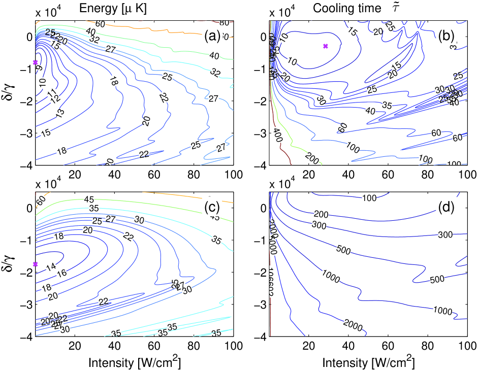
Figure 9: The energy of cooled ²⁴Mg atoms ((a) for $\theta=0$ and (c) for $\theta=\pi/2$) in $\mu K$ and the cooling time $\tilde{\tau}$ in dimensionless units ((b) for $\theta=0$ and (d) for $\theta=\pi/2$) in the dipole trap as function of pumping wave intensity and detunings obtained by the model based on decomposition of atomic density matrix on vibration state. Magenta cross define optimal parameters for minimum laser cooling energy of atoms and minimum cooling time for considered range of parameters.

For orthogonal orientation $\theta=\pi/2$ the minimum energy $E_{min}=13.2\mu K$ is reached for $I\simeq 0.1W/cm^{2}$ and detuning $\delta/\gamma\simeq-17500$, but the cooling time for these parameters is extremely large $\tau\gamma_{eff}\simeq 2\cdot 10^{5}$. For field parameters providing a reasonable cooling time $\tau\gamma_{eff}<100$ the energy above $60\mu K$ can be reached only (figure 9(c,d)).

3 Conclusion

We study laser cooling of ${}^{24}Mg$ atoms in the dipole trap with pumping field resonant to narrow $(3s3s)\,^{1}S_{0}\rightarrow\,(3s3p)\,^{3}P_{1}$ ($\lambda=457$ nm) optical transition and quench field resonant to $(3s3p)\,^{3}P_{1}\rightarrow\,(3s4s)\,^{1}S_{0}$. The effect of quenching we consider as widening of optical transition to $\gamma_{eff}$ only. We find the semiclassical model can not be used for description of laser cooling in this scheme. We suggest quantum models. The first one is based on the direct numerical solution of quantum kinetic equation for atom density matrix and the second is simplified model is based on decomposition of atom density matrix over vibration states in the dipole trap. The second model has limitations and describes the cooling of atoms on the lowest vibration levels only. The results of this model is differ from exact numerical solution for enough high intensity of pumping field (above 50$W/cm^{2}$ or Rabi above $25000\gamma$) when populations of the top vibration levels are not negligible, i.e. tunneling effects and above barrier motion of atoms can not be neglected. Nevertheless the simplified model well describes the laser cooling of atoms cooled to minimum energy. Additionally, the simplified model allows to estimate the cooling time. The parameters of pumping field for cooling to minimum energy do not coincide with conditions for fast cooling. We find parameters that allow cooling the atoms at reasonable cooling time $\tau\simeq 10/\gamma_{eff}$ (i.e. $\tau\simeq 0.5\,ms$ at $\gamma_{eff}=100\gamma$) to energy $E\simeq 12\,\mu K$.

In the considered models the steady state solution do not depends on $\gamma_{eff}$ while the cooling time is inversely proportional to $\gamma_{eff}$. The difference may appears for more complex model that takes into account pumping to level $(3s4s)\,^{1}S_{0}$ by quench field. We consider this question in the next paper.

The work was supported by Russian Science Foundation (project N 16-12-00054). V.I.Yudin acknowledges the support of the Ministry of Education and Science (3.1326.2017).

References

- [1] J. Dalibard and C. Cohen-Tannoudji, J. Opt. Soc. Am. B 6, 2023-2045 (1989).
- [2] J. Lawall, F. Bardou, B. Saubamea, K. Shimizu, M. Leduc, A. Aspect, and C. Cohen-Tannoudji, Two-dimensional subrecoil laser cooling, Phys. Rev. Lett. 73, 1915 (1994).
- [3] C. S. Adams, H. J. Lee, N. Davidson, M. Kasevich, and S. Chu, Evaporative cooling in a crossed dipole trap, Phys. Rev. Lett. 74, 3577 3580 (1995).
- [4] M. Kasevich and S. Chu, Laser cooling below a photon recoil with three-level atoms, Phys. Rev. Lett. 69, 1741 (1992).
- [5] J. Reichel, F. Bardou, M. Ben Dahan, E. Peik, S. Rand, C. Salomon, and C. Cohen-Tannoudji, Raman cooling of cesium below 3 nK: new approach inspired by Le vy flight statistics, Phys. Rev. Lett. 75, 4575 (1995).
- [6] A.P. Kulosa, D. Fim, K.H. Zipfel, S. Ruhmann, S. Sauer, N. Jha, K. Gibble, W. Ertmer, E.M. Rasel, M.S. Safronova, U.I. Safronova, S.G. Porsev, arXiv: 1508.01118v1, physics.atom-ph, 5 Aug 2015.
- [7] M. Riedmann, H. Kelkar, T. Wubbena, A. Pape, A. Kulosa, K. Zipfel, D. Fim, S. Ruhmann, J. Friebe, W. Ertmer, and E. Rasel, Phys. Rev. A 86, 043416 (2012).
- [8] O.N. Prudnikov, D. V. Brazhnikov, A. V. Taichenachev, V. I. Yudin, V I Yudin, A N Goncharov, Quantum Electronics, v. 46, Issue 7, p. 661-667, (2016)
- [9] E.A. Curtis, C.W. Oates, and L.Holberg Phys. Rev. A 64, 031403 (2001)
- [10] T. Binnewies, G. Wilpers, U. Sterr, J. Helmcke, T.E. Mehlstäbler, E.M. Rasel, and W. Ertmer Phys. Rev. Lett. 87, 123002 (2001)
- [11] T.E. Mehlstäbler, J. Keupp, A.Douillet, N. Rehbein, E.M. Rasel J.Opt.B: Quantum Semiclass. Opt. 5, S183 (2003)
- [12] V.V. Ivanov, S. Gupta Phys.Rev. A 84, 063417 (2011)
- [13] J. Javanainen Phys. Rev. A 44, 5857-5880 (1990)
- [14] O.N. Prudnikov, A. V. Taichenachev, A. M. Tumaikin and V. I. Yudin, JETP 98, 438-454 (2004)
- [15] Y. Castin and J. Dalibard Europhys. Lett., 14, 761-766 (1991)
- [16] O.N. Prudnikov, A.V. Taichenachev, A.V. Tumaikin, V.I. Yudin, Phys. Rev. A 75, 023413 (2007)
- [17] O. N. Prudnikov, R.Ya. Ilenkov, A. V. Taichenachev, A. M. Tumaikin, and V. I. Yudin, JETP v.112, pp.939-945 (2011)