How important is non-ideal physics in simulations of sub-Eddington accretion onto spinning black holes?

Abstract

Black holes with accretion rates well below the Eddington rate are expected to be surrounded by low-density, hot, geometrically thick accretion disks. This includes the two black holes being imaged at sub-horizon resolution by the Event Horizon Telescope. In these disks, the mean free path for Coulomb interactions between charged particles is large, and the accreting matter is a nearly collisionless plasma. Despite this, numerical simulations have so far modeled these accretion flows using ideal magnetohydrodynamics. Here, we present the first global, general relativistic, 3D simulations of accretion flows onto a Kerr black hole including the non-ideal effects most likely to affect the dynamics of the disk: the anisotropy between the pressure parallel and perpendicular to the magnetic field, and the heat flux along magnetic field lines. We show that for both standard and magnetically arrested disks, the pressure anisotropy is comparable to the magnetic pressure, while the heat flux remains dynamically unimportant. Despite this large pressure anisotropy, however, the time-averaged structure of the accretion flow is strikingly similar to that found in simulations treating the plasma as an ideal fluid. We argue that these similarities are largely due to the interchangeability of the viscous and magnetic shear stresses as long as the magnetic pressure is small compared to the gas pressure, and to the sub-dominant role of pressure/viscous effects in magnetically arrested disks. We conclude by highlighting outstanding questions in modeling the dynamics of low collisionality accretion flows.

1 Introduction

Supermassive black holes (SMBHs) are found at the center of most galaxies, and a majority of these black holes are accreting much slower than the Eddington accretion rate (Ho, 2009). This is in particular the case for the two SMBHs with the largest angular size on the sky: SgrA^∗, at the center of the Milky Way, and the black hole at the center of M87. These black holes are important targets for high-resolution imaging experiments such as the Event Horizon Telescope (Doeleman et al., 2009) and Gravity (Eisenhauer et al., 2008), which may provide us with constraints on the properties of SMBHs and on the behavior of accretion flows in the immediate neighborhood of a black hole. Accordingly, it is important to be able to quantitatively model accretion flows close to slowly accreting SMBHs.

Accretion flows at low accretion rates are expected to be geometrically thick and optically thin. Both theoretical models (Yuan & Narayan, 2014) and numerical simulations (Koide et al., 1999; De Villiers et al., 2003; McKinney & Gammie, 2004) of these radiatively inefficient accretion flows (RIAF) indicate that the density and temperature in the disk are such that the mean free path for Coulomb interactions between charged particles is much larger than the typical size of the system, $\sim GM/c^{2}$ (with $G$ the gravitational constant, $M$ the black hole mass, and $c$ the speed of light). We then expect the accreting matter to be nearly collisionless. This raises questions about the accuracy of existing numerical simulations, which treat the accretion flow as an ideal fluid.

Shearing-box simulations using particle-in-cell methods have shown that the situation is probably not as dire as it might seem. Wave-particle interactions due to velocity-space instabilities effectively increase the collision rate of particles, and limit the amplitude of non-ideal effects (Kunz et al., 2014; Riquelme et al., 2015; Sironi & Narayan, 2015; Kunz et al., 2016). The impact of those instabilities is also verified observationally in the solar wind (Kasper et al., 2002; Hellinger et al., 2006). More specifically, the phase space of solar wind particles appears to be bounded by the instability thresholds of the mirror and firehose instabilities, which limit the pressure anisotropy to be of the same order as the magnetic pressure.

Global simulations of an accretion disk made of a collisionless plasma would require time evolution of the 6D distribution functions of ions and electrons. This is beyond the reach of current numerical simulations. However, the effective collisionality provided by wave-particle interactions justifies modeling the accretion flow as a weakly collisional plasma, in which non-ideal effects are treated as a perturbation of the ideal fluid model.

Non-ideal effects could play a number of potentially important roles. First, they may affect the dynamics of the disk, i.e. the bulk motion of the charged particles. Second, they may lead to different temperatures for the ions and electrons. And finally, they may cause both ions and electrons to have non-thermal distribution functions. The second and third points probably do not directly affect the dynamics of the disk, but may be important to its radiative properties, which are largely determined by the energy spectrum of the electrons.

In this work, we focus on the impact of non-ideal effects on the dynamics of accretion disks at highly sub-Eddington accretion rates. In particular, we include for the first time in 3D global simulations the two non-ideal effects most likely to affect the disk dynamics: the anisotropy between the pressure parallel and perpendicular to the magnetic field, and the presence of a heat flux along magnetic field lines. To do this, we rely on our recently developed general relativistic model for the evolution of the pressure anisotropy and heat flux in a weakly collisional plasma (Chandra et al., 2015).

In previous axisymmetric global simulations of accretion disks, we demonstrated that the pressure anisotropy rapidly grows and becomes comparable to the magnetic pressure, saturating at the threshold of the mirror instability (Foucart et al., 2016). However, in axisymmetry, the turbulent cascade transfers energy to longer wavelengths, and cannot be self-consistently sustained. To study a steady-state accretion flow, we require the 3D simulations presented here.

In Sec. 2, we review the main features of the extended magnetohydrodynamics model used to describe the plasma in our simulations. Sec. 3 discusses our choice of initial conditions and numerical methods. Sec. 4 provides a detailed comparison of simulations with and without non-ideal effects for an accretion disk in which the magnetic pressure of the relativistic polar jet does not affect the dynamics of the disk (the standard, or SANE configuration), Sec. 5 shows results for a magnetically arrested disk (MAD), in which the magnetic pressure of the jet nearly balances the pressure of the infalling gas. Secs. 4-5 thus provide us with an opportunity to study non-ideal effects in very different physical regimes. Finally, we conclude and discuss the current limitations of our model and potential future work in Sec. 6.

In the following sections, we use the length unit $r_{g}=GM/c^{2}\sim 0.04\left(\frac{M}{4\times 10^{6}M_{\odot}}\right)\,{\rm AU}$ and time unit $t_{g}=GM/c^{3}\sim 20\left(\frac{M}{4\times 10^{6}M_{\odot}}\right)\,{\rm s}$.

2 Extended Magnetohydrodynamics model

We describe the nearly collisionless plasma as a well-magnetized, weakly collisional plasma, following the general relativistic model proposed in Chandra et al. (2015). In this limit, we assume that the Larmor radius of charged particles is very small compared to the typical length scale of the accretion disk ($L\sim r$, the distance to the center of the black hole). This is nearly certain to be the case in practice, as the disk is expected to be unstable to the magnetorotational instability (MRI, Balbus & Hawley, 1991). Even a small seed magnetic field would grow exponentially on a timescale comparable to the orbital time scale of the disk. We also assume that deviations from an ideal fluid are small, so that non-ideal effects can be treated perturbatively. While not intuitively obvious, this assumption is supported by particle-in-cell simulations showing that wave-particle interactions generated by velocity-space instabilities (e.g. firehose, mirror) create an effective collision rate in the system (Kunz et al., 2014; Riquelme et al., 2015; Sironi & Narayan, 2015; Kunz et al., 2016). Under these assumptions, we model the plasma using an extended magnetohydrodynamics (EMHD) model which is a generalization of Braginskii’s theory for magnetized, weakly collisional plasmas (Braginskii, 1965), modified to make the theory stable and causal within a general relativistic framework.

We start from the ideal description of a fluid of density $\rho$, internal energy density $u$, pressure $P$, and 4-velocity $u^{\mu}$, with a magnetic field 4-vector $b^{\mu}$ (in the fluid frame), and a known spacetime metric $g_{\mu\nu}$. The ideal part of the stress-energy tensor is then

$$T^{\mu\nu}_{\rm ideal}=(\rho+u+b^{2}+P)u^{\mu}u^{\nu}+(P+\frac{b^{2}}{2})g^{\mu\nu}-b^{\mu}b^{\nu},$$ (1)

with $b^{2}=b^{\mu}b_{\mu}$ being twice the magnetic pressure; we have absorbed the factor of $(4\pi)^{-1/2}$ into the definition of the magnetic field. Non ideal effects are modeled through a heat flux constrained to be along magnetic field lines ($q^{\mu}=qb^{\mu}$), and an anisotropy between the pressure parallel and perpendicular to the magnetic field lines, $P_{\parallel}=P-\frac{2}{3}\Delta P$ and $P_{\perp}=P+\frac{1}{3}\Delta P$. The full stress-energy tensor is then written as

$$T^{\mu\nu}=T^{\mu\nu}_{\rm ideal}+q^{\mu}u^{\nu}+q^{\nu}u^{\mu}+\Pi^{\mu\nu},$$ (2)

where the anisotropic shear stress $\Pi^{\mu\nu}$ is related to the pressure anisotropy by

$$\Pi^{\mu\nu} = -\Delta P\left(\hat{b}^{\mu}\hat{b}^{\nu}-\frac{1}{3}h^{\mu\nu}\right),$$ (3)

$$h^{\mu\nu} = g^{\mu\nu}+u^{\mu}u^{\nu},$$ (4)

with $\hat{b}^{\mu}=b^{\mu}/b$. In Braginskii’s theory, the heat flux and pressure anisotropy are simply proportional to, respectively, the temperature gradient along magnetic field lines, and the projection of the velocity shear tensor onto the magnetic field. However, in general relativity, such a prescription violates causality. Instead, we have to promote $q$ and $\Delta P$ to evolved variables, and drive them towards their desired value

$$q_{0} = \rho\chi\hat{b}^{\mu}\left(\nabla_{\mu}\Theta+\Theta u^{\nu}\nabla_{\nu}u_{\mu}\right),$$ (5)

$$\Delta P_{0} = 3\rho\nu\left(\hat{b}^{\mu}\hat{b}^{\nu}\nabla_{\mu}u_{\nu}-\frac{1}{3}\nabla_{\mu}u^{\mu}\right),$$ (6)

which are covariant versions of the heat flux and pressure anisotropy in Braginskii’s theory. Here, $\Theta=kT/(m_{p}c^{2})$ is the dimensionless temperature, $m_{p}$ the proton mass, $\chi$ the thermal diffusivity, and $\nu$ the kinematic viscosity.

The first 8 evolution equations of the EMHD model are easily obtained from the conservation equations

$$\nabla_{\mu}(\rho u^{\mu}) = 0,$$ (7)

$$\nabla_{\mu}T^{\mu\nu} = 0,$$ (8)

and from Maxwell’s equation

$$\nabla_{\mu}(b^{\mu}u^{\nu}-b^{\nu}u^{\mu})=0.$$ (9)

We also use the simple equation of state

$$P=\rho\Theta=(\Gamma-1)u,$$ (10)

with $\Gamma$ the polytropic index of the fluid. In the simulations, we will consider an ideal gas of non-relativistic particles, for which $\Gamma=5/3$. This choice is reasonable as long as the electron temperature $T_{e}$ is much lower than the ion temperature $T_{p}$, and $\Theta_{p}<1$. This is expected to be the case for slowly accreting supermassive black holes such as SgrA^∗.

For the non-ideal sector, we evolve the rescaled variables

$$\tilde{q} = q\sqrt{\frac{\tau_{R}}{\rho\chi\Theta^{2}}},$$ (11)

$$\Delta\tilde{P} = \Delta P\sqrt{\frac{\tau_{R}}{\rho\nu\Theta}},$$ (12)

according to

$$\nabla_{\mu}(\tilde{q}u^{\mu}) = -\frac{\tilde{q}-\tilde{q}_{0}}{\tau_{R}}+\frac{\tilde{q}}{2}\nabla_{\mu}u^{\mu},$$ (13)

$$\nabla_{\mu}(\Delta\tilde{P}u^{\mu}) = -\frac{\Delta\tilde{P}-\Delta\tilde{P}_{0}}{\tau_{R}}+\frac{\Delta\tilde{P}}{2}\nabla_{\mu}u^{\mu},$$ (14)

with $\tau_{R}$ a relaxation timescale yet to be determined. The exact choice of evolved variables and evolution equations are driven in part by numerical considerations, and in part by the requirement that the model satisfies the second law of thermodynamics. The system of equations defined by Eqs (7,8,9,13,14) remains causal and stable as long as $\tau_{R}/\chi$ and $\tau_{R}/\nu$ are not too small, in a sense discussed in more detail in Chandra et al. (2015).

Note that the EMHD model used here includes an explicit treatment of some quantities associated with dissipative processes (field aligned thermal diffusion and viscosity) but relies on the numerical diffusion for the treatment of others (resistivity, cross-field viscosity and cross-field thermal diffusion). The motivation for this is that the transport along field lines is expected to be particularly large and important in low-collisionality plasmas. It is worth bearing in mind, however, that ideal MHD simulations have demonstrated the importance of an explicit treatment of isotropic viscosity and resistivity for the saturation of the MRI in some regimes (Lesur & Longaretti, 2007; Fromang et al., 2007). This is not included in our models but is an important extension to consider in future work (see Sec. 6.1).

This leaves us with 3 free model parameters: $\tau_{R}$, $\chi$, and $\nu$, which should be determined from kinetic theory. We can interpret $\tau_{R}$ as the effective mean-free time between collisions, which in our applications is the effective mean free time for wave-particle scatterings. In the absence of plasma instabilities, a reasonable first guess for $\tau_{R}$ in an accretion torus is the dynamical timescale, $\tau_{d}=\sqrt{r^{3}/(GM)}$. We can also estimate $\chi$ and $\nu$ from their value in non-relativistic collisional theory, $\chi=\phi c_{s}^{2}\tau_{R}$ and $\nu=\psi c_{s}^{2}\tau_{R}$, with $\phi$ and $\psi$ dimensionless constants of order unity and $c_{s}=\sqrt{\Gamma P/(\rho+\Gamma u)}$ the sound speed. Here, we choose $\psi=1$ and $\phi=1$.

When $\Delta P$ becomes comparable to the magnetic pressure, however, the relaxation time $\tau_{R}$ is probably reduced by the onset of plasma instabilities. Particle-in-cell simulations (Kunz et al., 2014; Riquelme et al., 2015) have shown that the ions are unstable to the firehose instability if $\Delta P<-b^{2}\equiv\Delta P_{\rm firehose}$ and to the mirror instability if

$$\Delta P>\Delta P_{\rm mirror}=\frac{b^{2}}{2}\frac{P_{\parallel}}{P_{\perp}}.$$ (15)

Once the pressure anisotropy reaches these thresholds, we expect the growth of plasma instabilities, and the saturation of $\Delta P$ at the instability threshold. Similarly, the heat flux cannot exceed the free-streaming value of $|q|=\rho c_{s}^{3}$. In the EMHD model, we can attempt to mimic the effects of plasma instabilities by modifying $\tau_{R}$ in such a way that $\Delta P$ remains within the expected stability region, and $|q|<\rho c_{s}^{3}$. This can be done if we choose, for example,

$$\tau_{R}=\tau_{d}\times(f_{\rm min}+f(|q|,\rho c_{s}^{3})\times f(\Delta P,\Delta P_{\rm firehose})\times f(\Delta P,\Delta P_{\rm mirror})$$ (16)

with

$$f(x,x_{\rm max}) = \frac{1}{1+e^{g(x,x_{\rm max})}},$$ (17)

$$g(x,x_{\rm max}) = \frac{1}{\Delta x}\frac{x-x_{\rm max}}{x_{\rm max}}.$$ (18)

In our simulations, we use this prescription with $\Delta x=0.01$ and $f_{\rm min}=10^{-5}$ (the exact form of the function $f$ sets how far $\Delta P$ and $q$ can grow above their maximum allowed value, and is chosen to provide a fairly strict limit in our model).

When analyzing the results of our simulations, a few analytical properties of the EMHD model are good to keep in mind:

• For a Keplerian velocity profile and a plasma parameter $\beta=2P/b^{2}\gtrsim 1$, we expect $\Delta P\sim b^{2}/2$ and $\tau_{R}\sim\tau_{d}/\beta$ (Kunz et al., 2014). A priori, there is no guarantee that this is also true for a turbulent flow in a magnetized disk. However, we have already shown that this prediction holds for turbulent accretion flows in axisymmetry (Foucart et al., 2016), and the same is true for the full 3D simulations presented here. Because of this, the arbitrary choices made for the values of $\phi$ and $\psi$ are relatively unimportant. Instead, the mirror instability threshold $\Delta P_{\rm mirror}\sim b^{2}/2$ sets $\Delta P$.

• $\Delta P$ and $q$ are driven towards their Braginskii values on a timescale $\tau_{R}$ which is, at most, comparable to the orbital time scale, and shorter than the time scale for the growth of the MRI. This means that if the evolution of the magnetic field is mostly driven by the growth of the MRI, $\Delta P$ effectively reacts nearly instantaneously to changes in the magnetic pressure. The time evolution equations for $\Delta P$ and $q$ are necessary to guarantee causality, but are not otherwise critical.

• The off-diagonal contributions of the viscous stress $\Pi^{\mu}_{\nu}$ and of the magnetic stress $T^{\mu}_{\nu,\rm mag}$ to the stress-energy tensor $T^{\mu}_{\nu}$ have some interesting similarities:

  $$T^{\mu}_{\nu,\rm mag} = -b^{2}\left(\hat{b}^{\mu}\hat{b}_{\nu}-\frac{h^{\mu}_{\nu}}{2}-\frac{u^{\mu}u_{\nu}}{2}\right),$$ (19)

  $$\Pi^{\mu}_{\nu} = -\Delta P\left(\hat{b}^{\mu}\hat{b}_{\nu}-\frac{1}{3}h^{\mu}_{\nu}\right).$$ (20)

  For $\Delta P=b^{2}$, the off-diagonal components of the viscous and magnetic stresses as measured in the orthonormal frame comoving with the fluid are equal. In particular, this is true for the $r-\phi$ component of the stress-energy tensor in the comoving frame, which dictates angular momentum transport in the disk. On the other hand, the diagonal components of the magnetic and viscous stresses in the comoving frame, which describe the energy density and isotropic pressure, differ.

These properties of the EMHD model will play an important role in the interpretation of our simulation results in Sections 4-5.

3 Numerical Setup

3.1 Initial Conditions

For this first exploration of the effect of a pressure anisotropy and heat conduction on the dynamics of an accretion torus, we consider initial conditions widely used in the literature: the hydrostatic equilibrium solution for a torus of constant specific entropy orbiting a rotating black hole, due to Fishbone & Moncrief (1976). Ideal MHD (IMHD) simulations of accretion tori have already shown that there are at least two distinct types of accretion onto black holes: the so-called SANE (Standard And Normal Evolution, Narayan et al. 2012) and MAD (Magnetically Arrested Disk, Bisnovatyi-Kogan & Ruzmaikin 1974, 1976; Narayan et al. 2003; Igumenshchev et al. 2003; Igumenshchev 2008; Tchekhovskoy et al. 2011; Tchekhovskoy & McKinney 2012) configurations. In a MAD disk, the magnetic flux threading the black hole horizon becomes so large that the magnetic pressure of the jet can temporarily stop the flow of matter into the black hole. In a SANE disk, on the other hand, the magnetically-dominated polar regions do not significantly affect the dynamics of the accretion flow. Absent large-scale poloidal magnetic flux dynamo, magnetic flux conservation implies that the magnetic field seeded in the initial equilibrium torus determines the large-scale magnetic flux that can be accumulated by the black hole, and thus the resulting type of the steady-state accretion flow. Here, we will consider two sets of initial conditions, one leading to SANE and one to MAD accretion flows. Whether astrophysical accretion disks around supermassive black holes are in a MAD or SANE state remains an open question. There are observational indications that dynamically important magnetic fields might be present in active galactic nuclei (Zamaninasab et al., 2014; Ghisellini et al., 2014), tidal disruption events (Tchekhovskoy et al., 2014), and gamma-ray bursts (Tchekhovskoy & Giannios, 2015).

The Fishbone-Moncrief solution is entirely defined by the dimensionless spin of the black hole ($a/M_{\rm BH}$), the inner radius of the torus ($r_{\rm in}$) and radius of the pressure maximum in the disk ($r_{\rm max}$), the polytropic index used in the equation of state $\Gamma=5/3$, and the entropy $P/\rho^{\Gamma}=0.0043$. For the SANE simulation, we choose $a/M_{\rm BH}=0.9375$, $r_{\rm in}=6r_{g}$, and $r_{\rm max}=12r_{g}$. For the MAD simulation, we have $a/M_{\rm BH}=0.5$, $r_{\rm in}=15r_{g}$, and $r_{\rm max}=32r_{g}$. As the mass scale within the accreting matter is arbitrary, we choose it so that $\max{(\rho)}=1$ in the initial torus.

We seed the tori with a weak poloidal magnetic field. The magnetic field in the inertial frame, $B^{i}$, is derived from the vector potential $A^{\mu}$ using $B^{i}=b^{i}u^{t}-b^{t}u^{i}=\epsilon^{ijk}\nabla_{j}A_{k}$, with $\epsilon_{ijk}$ the Levi-Civita symbol. For the SANE disk, we set $A_{\phi}=A_{0}\max(\rho-0.2,0)$, with the constant $A_{0}$ chosen so that the minimum value of $\beta=2P/b^{2}$ in the disk is $\beta_{\rm min}=15$. This guarantees that the magnetic field is weak enough to avoid disrupting the equilibrium torus, but strong enough to allow us to resolve the fastest growing mode of the magnetorotational instability (MRI). For the MAD disk, we set $A_{\phi}=A_{0}\rho^{2}r^{4}$, with $A_{0}$ such that $\max{(P)}=100\max{(b^{2}/2)}$. As we will see, this is sufficient to lead to the accumulation of a large magnetic flux on the black hole horizon, and a MAD accretion flow with $\beta\sim 1$. We also add a random perturbation to the internal energy density, $u=u_{\rm eq}+\delta u$, with $u_{\rm eq}$ the energy density in the Fishbone-Montcrief solution, and $\delta u$ drawn from a uniform distribution covering $[-0.04u_{\rm eq},0.04u_{\rm eq}]$. This perturbation will seed turbulent motion in the disk. The pressure anisotropy and heat flux are initialized to $\Delta P=q=0$. The initial density and poloidal magnetic field of the SANE disk are shown in Fig. 1.

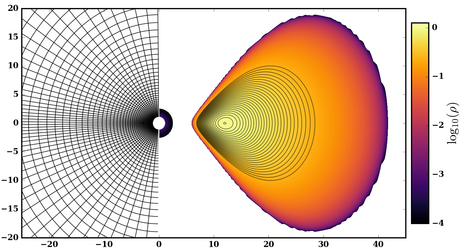
Figure 1: Vertical slice through the numerical grid (left, with each cell actually representing a $5x5$ group of cells at our highest resolution), and the initial torus for the SANE simulations (right, the color scale shows the fluid density, while solid black lines follow the seed magnetic field lines.).

3.2 Numerical methods

To evolve the EMHD model we developed a new code, grim, described in Chandra et al. (2017). Evolving the EMHD model requires the use of implicit-explicit time stepping methods, instead of the purely explicit methods used to evolve the general relativistic equations of ideal MHD. Indeed, the dissipative quantities in the EMHD model, namely the heat flux $q$ and the pressure anisotropy $\Delta P$, are sourced by spatio-temporal gradients of the thermodynamic variables. In grim, all flux terms in the equations are treated explicitly, while some local source terms are treated implicitly. Accordingly, neighboring points are only coupled through terms treated explicitly, and the implicit solve can be done grid point by grid point. At each point and for each time step, we have to solve a set of non-linear implicit equations for 7 evolved variables. The evolution of the magnetic field can be treated explicitly, and fully decouples from the implicit solve. Numerical fluxes on cell faces are computed with left- and right-biases stencils using the PPM reconstruction (Colella & Woodward, 1984), with a Local Lax-Friedrich approximate Riemann solver to reconstruct the fluxes from the left and right states on each face. Due to the use of implicit-explicit time stepping, the EMHD model is significantly more expensive to evolve than IMHD. The simulations presented here can perform $\sim 10^{5}$ zone-cycles per second and per GPU node on the TACC Stampede cluster, about two orders of magnitude slower than state-of-the-art explicit evolutions on the same infrastructure (Liska, Tchekhovskoy, et al., in preparation).

When evolving the equations of IMHD or EMHD in regions with relativistic velocities or with large magnetic fields, small discretization errors can lead to large numerical errors in energetically subdominant physical variables (e.g. the velocity in magnetically dominated regions). To avoid this issue, we implement techniques commonly used in IMHD simulations, imposing an upper bound on the Lorentz factor $\gamma$, and lower bounds on the density and internal energy of the fluid. In particular, we require $\gamma<10$, $\rho>10^{-3}(r/r_{\rm in})^{(-5/2)}$, $u>10^{-5}(r/r_{\rm in})^{(-5/2)}$, $\rho>0.1b^{2}$, and $u>0.002b^{2}$. When these conditions are violated, we reduce the velocity and increase $\rho$ or $u$ as needed. The addition of mass or energy is performed in the drift frame of the plasma, as described in Ressler et al. (2017). At the inner boundary, these conditions are identical to those used in our previous axisymmetric simulations (Foucart et al., 2016). Farther away, the density and internal energy floors decrease faster with radius than in previous simulations, as we found that in long 3D simulations higher floors could impact the evolution of low-density outflows produced by the disk.

We impose reflecting boundary conditions at the poles, an outflow boundary condition at the outer radial boundary ($u^{r}>0$), and periodic boundary conditions in the azimuthal direction. To avoid instabilities at the poles we also correct the value of the primitive variables in the two cells closest to the polar axis. In these cells, the variables $(u^{\theta},b^{\theta},\Delta P,q)$ are assumed to go to zero linearly with the polar angle $\theta$, while the rest of the hydrodynamic variables are assumed to be constant. We do not modify the magnetic fields.

3.3 Coordinates and grid structure

The evolution equations for the EMHD model are solved on a 3-dimensional domain in modified Kerr-Schild coordinates $(t,a,b,c)$, related to the usual Kerr-Schild coordinates $(t,r,\theta,\phi)$ by the maps

$$r = \exp{a}$$ (21)

$$\tilde{\theta} = \arccos{\big{(}[1-f(r)]\mu_{\rm Ref}+f(r)\mu_{\rm uni}\big{)}}$$ (22)

$$\mu_{\rm ref} = \cos{[\pi b+0.35\sin{(2\pi b)}]}$$ (23)

$$\mu_{\rm uni} = \cos{[\pi b]}$$ (24)

$$\phi = 2\pi c$$ (25)

$$f(r) = \frac{r_{\rm in}}{r}$$ (26)

and a map $\tilde{\theta}\rightarrow\theta$ which derefines the grid in the $\theta$ direction close to the polar boundary. The exact form of this map is provided in the appendix. The resulting grid structure is shown in Fig. 1.

The mapping $\mu_{\rm ref}$ is taken from Gammie et al. (2003), and aims at focusing resolution close to the equatorial plane of the disk, where the MRI is more difficult to resolve. We switch to a uniform mapping $\mu_{\rm uni}$ close to the inner boundary in order to avoid limiting the time step by the use of a very small grid spacing in the $\theta$ direction on the boundary. The mapping from $\tilde{\theta}$ to $\theta$ serves a similar purpose: by derefining the grid close to the polar boundary, we avoid very small grid spacings in the azimuthal direction close to the axis. The map parameters are chosen in order to maximize the minimum grid spacing across the entire domain.

3.4 Resolution and convergence

We evolve the SANE torus at two resolutions for both the IMHD and EMHD model. The high resolution simulations use $256\times 256\times 128$ cells along the $(a,b,c)$ directions. The low resolution simulations use $128\times 128\times 64$ cells. For the MAD disk, we use $256\times 128\times 64$ grid points and evolve the system with both the EMHD and IMHD models. In all simulations, we place the inner edge of the grid at $r_{\rm in}=0.85r_{\rm H}$, with $r_{\rm H}=r_{g}(1+\sqrt{1-a^{2}})$ the radius of the black hole horizon. This guarantees 6 grid cells inside the horizon at low resolution. The outer edge of the grid is at $r_{\rm out}=55r_{g}$ for the SANE disk, and $r_{\rm out}=3000r_{g}$ for the MAD disk. Finally, all SANE simulations are evolved for a time $\Delta t=6000t_{g}$, and all MAD simulations for $\Delta t=14000t_{g}$.

Before further analysis of our results, it is useful to note which effects our simulations can resolve. For the SANE disk, we rely for this analysis on the simulations at two numerical resolutions performed here, and on pre-existing ideal MHD simulations. In particular, we can compare our results with the detailed analysis of an ideal MHD accretion flow presented in Shiokawa et al. (2012).  Shiokawa et al. (2012) showed that simulations with numerical resolution comparable to our highest resolution were well converged for some global quantities (magnetization of the disk, temperature, accretion rate), and captured the scale of the fastest growing mode of the MRI. However, they only marginally resolved the azimuthal correlation length of the fluid variables (density, internal energy), and underresolved the azimuthal correlation length of the magnetic field. We find that our simulations have very similar properties. In particular, the differences observed in global, time-averaged disk quantities between our two resolutions are comparable to the results at similar resolution in Shiokawa et al. (2012). We also find that, at our highest resolution, the azimuthal correlation length of the fluid quantities is $\sim 7$ grid spacings, while the azimuthal correlation length of the magnetic field is only $\sim 4$ grid spacings. We do not observe significant differences between the convergence properties of the EMHD and IMHD models.

From these results, we infer that our simulations allow us to do a direct comparison of the EMHD and IMHD models for a steady-state, SANE accretion flow. We can compare time-averaged profile of the accretion flow, and the dynamics of the disk, but will not fully capture the azimuthal variations in the disk or the turbulent cascade driven by the MRI. In that respect, our simulations are largely similar to existing IMHD results at similar resolution.

Because of the stronger magnetic fields in the MAD disks, their resolution requirements are less stringent than for SANE disks. In particular, with rather low resolutions, it is possible to resolve the wavelength of the fastest growing mode of the MRI in the MAD disk proper. Even though higher values of the azimuthal resolution, $N_{\phi}$, lead to the emergence of smaller-scale structure in the MAD disks, their steady state properties appear to be rather insensitive to the resolution, with $N_{\phi}=64$ and $128$ giving qualitatively similar time-average disk properties (Tchekhovskoy et al., 2011). However, higher $\theta$-resolutions might be beneficial for resolving the innermost regions of the MAD disks, in the immediate vicinity of the event horizon, where the disks are strongly vertically compressed by the magnetic pressure of the polar jets.

4 Standard Disk Results

4.1 Overview of the disk evolution

The qualitative evolution of the standard (SANE) accretion flow studied here is largely independent of the underlying fluid model (IMHD vs EMHD), or of the numerical resolution used in the simulation. The initial torus is in hydrostatic equilibrium, but unstable to the growth of the magnetorotational instability (MRI). Accordingly, the MRI grows from the seed perturbations in our initial conditions, on a timescale comparable with the orbital timescale of the disk ($\sim 250t_{g}$ at the pressure maximum of the initial torus). The MRI drives turbulence in the disk, causing outward angular momentum transport, the accretion of matter onto the black hole, and heating of the accretion flow. The initial accretion torus then acts as a large matter reservoir feeding a quasi-steady state accretion flow onto the black hole. Steady-state is typically reached on a timescale $\tau_{st}(r)\sim\tau_{d}\alpha^{-1}\left(r/H\right)^{2}$, the “viscous” timescale of the disk, with $\alpha\sim 0.01-0.1$ and $H$ the scale height of the disk. In steady-state, a thick, turbulent accretion disk fills the equatorial region, while the polar regions are magnetically dominated.

The initial transient leading to the formation of a steady-state accretion flow is mostly determined by our choice of initial conditions, and the exact realization of the seed perturbation. We will largely ignore that phase in our analysis. The time-averaged properties of the steady-state accretion flow, on the other hand, are more robust, and thus more interesting to study. This does not mean, however, that our chosen initial conditions no longer have an impact. In particular, there are two important aspects of our initial conditions which should be kept in mind when analyzing our results.

The first is that the initial equilibrium torus for the SANE simulation is quite compact, and resides deeply in the gravitational potential of the black hole. This means that the accretion flow at distances $r\gtrsim 10r_{g}$ remains, at all times, solely a consequence of the initial conditions. Additionally, disk outflows are artificially suppressed in this configuration: all of the matter starts with a relatively high binding energy, and close to the black hole. The second important impact of the initial conditions is the evolution of the net magnetic flux threading the black hole horizon, which determines whether the disk ends up in the SANE or MAD configuration. We discuss an accretion flow reaching the MAD state in Sec. 5.

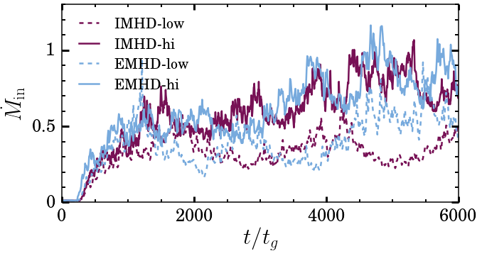
Figure 2: Accretion rate across the black hole horizon as a function of time, for the EMHD and IMHD SANE models at low and high resolution. Note the very similar accretion history for the two high-resolution runs.

The rate $\dot{M}$ of accretion of matter onto the black hole for each of our 4 SANE simulations is shown in Fig. 2. In all cases, accretion begins after a time delay consistent with the MRI growth timescale, then reaches a turbulent quasi-steady state on a timescale of the order of the viscous timescale at the innermost stable circular orbit of the black hole. In the rest of this paper, we focus our SANE disk simulation analysis on the time period $(4000-6000)t_{g}$, when we expect quasi-steady accretion for $r\lesssim 7r_{g}$. We see that during that period, the average accretion rates of the high-resolution IMHD and EMHD simulations are very similar, which will facilitate comparisons between the two models. The low-resolution simulations have more significant differences in their accretion history, but these remain consistent with random variations of the accretion rate over the relatively small timescales that we can afford to simulate.

4.2 Steady-state disk profile

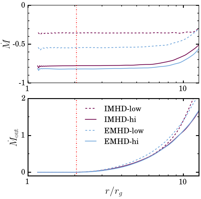
Figure 3: Time averaged mass accretion rate $\dot{M}$ as a function of radius for the SANE accretion flow. The vertical dot-dashed red-lines show the location of the innermost stable circular orbit (ISCO) for point-particles in prograde orbits. Top: Net accretion for the IMHD and EMHD models at two resolutions. We see that all disks reach a quasi steady-state up to $r\sim(8-9)r_{g}$. Bottom: Total outgoing mass flux for the IMHD and EMHD models at two resolutions (i.e. integrating the radial mass flux solely over regions in which it is positive). This mass flux is due to turbulent, outwardly directed motion of gas in the disk.

Fig. 3 shows the net accretion rate $\dot{M}$, and the outgoing mass flux $\dot{M}_{\rm out}$ as a function of radius, time-averaged over the window $t=(4000-6000)t_{g}$. $\dot{M}_{\rm out}$ is computed by only integrating the radial mass flux over fluid elements with outgoing radial velocities. The constant $\dot{M}$ profiles for $r\lesssim 7r_{g}$ confirm that we have reached a quasi-steady state in that region, and that we are in fact very close to steady-state up to $r\sim 9r_{g}$. Nearly all of the matter is flowing inwards for $r\lesssim(3-4)r_{g}$, while at larger radii turbulent motions in the disk cause some material to move outwards, with $\dot{M}_{\rm out}\sim|\dot{M}|$ in the outermost regions of the steady-state accretion flow. As shown by the velocity streamlines in Fig. 4, we do not observe any spatial region with steady-state outflows, confirming the absence of any strong disk wind in the compact SANE disk considered here.

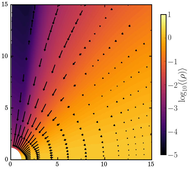
Figure 4: Density and velocity of the SANE accretion flow in the EMHD model, averaged over the azimuthal direction and within the time window $t=(4000-6000)t_{g}$. There are no steady-state outflows in this model (the outflows at $r>10r_{g}$ are not in the steady-state region). All distances are in units of $r_{g}=GM/c^{2}$.

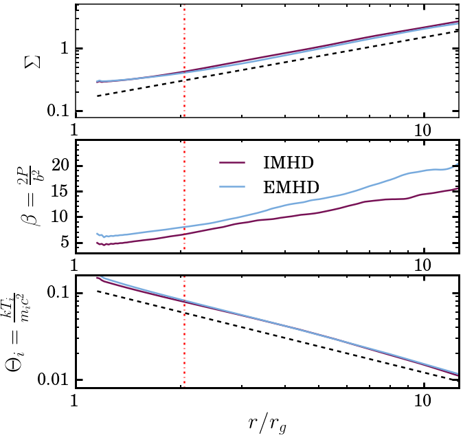
Figure 5: Surface density $\Sigma$, plasma parameter $\beta=2P/b^{2}$, and dimensionless ion temperature $\Theta_{i}$ as a function of radius for the SANE configuration using the EMHD and IMHD models. $\Sigma$ is averaged over time and the azimuthal direction. For $\beta$, we compute the ratio of the density-weighted averages of the gas pressure and magnetic pressure, while we directly compute the density-weighted average value of $\Theta$. $\beta$ is higher in the EMHD simulations, while the gas temperature and surface density are nearly identical in both models. The dashed black lines show power laws $\Sigma\propto r$ and $\Theta_{i}\propto r^{-1}$, while the dot-dashed red-lines show the location of the ISCO.

Some of the most important properties of the accretion flow in steady-state are shown in Fig. 5, which shows radial profiles of the surface density $\Sigma$, ion temperature $\Theta_{i}$, and plasma parameter $\beta=2P/b^{2}$ (the ratio of the gas to magnetic pressure). These profiles are averaged over the time window $t=(4000-6000)t_{g}$, and over the azimuthal angle. They are also integrated over the polar angle $\theta$. Unless otherwise specified, all figures show results for the higher resolution simulations. We see that the surface density and ion temperature in the disk are nearly identical for the IMHD and EMHD models. They also closely follow the power-law profiles $\Sigma\propto r$ and $\Theta_{i}\propto r^{-1}$. The latter is consistent with the conversion of gravitational potential energy into thermal energy, as expected for a radiatively inefficient disk. On the other hand, when it comes to the plasma $\beta$, the IMHD and EMHD model differ: the disk is more strongly magnetized in ideal MHD, with $\beta_{\rm EMHD}\approx(1.2-1.4)\beta_{\rm IMHD}$.

Overall, the most striking feature of the steady-state disk profiles are the similarities between the IMHD and EMHD simulations, shown for the fluid variables ($\rho$, $\Theta_{i}$) in the radial profiles shown in Fig. 5, but also verified for angular profiles at fixed radius, or for the azimuthal correlation length of the fluid variables and of the magnetic field. Despite the significant pressure anisotropy in the disk (discussed below), the steady-state accretion flow is remarkably independent of the choice of fluid model. The only difference which cannot be explained by random fluctuations in the accretion flow is the lower magnetic field strength in the EMHD simulation.

4.3 Pressure anisotropy and heat conduction

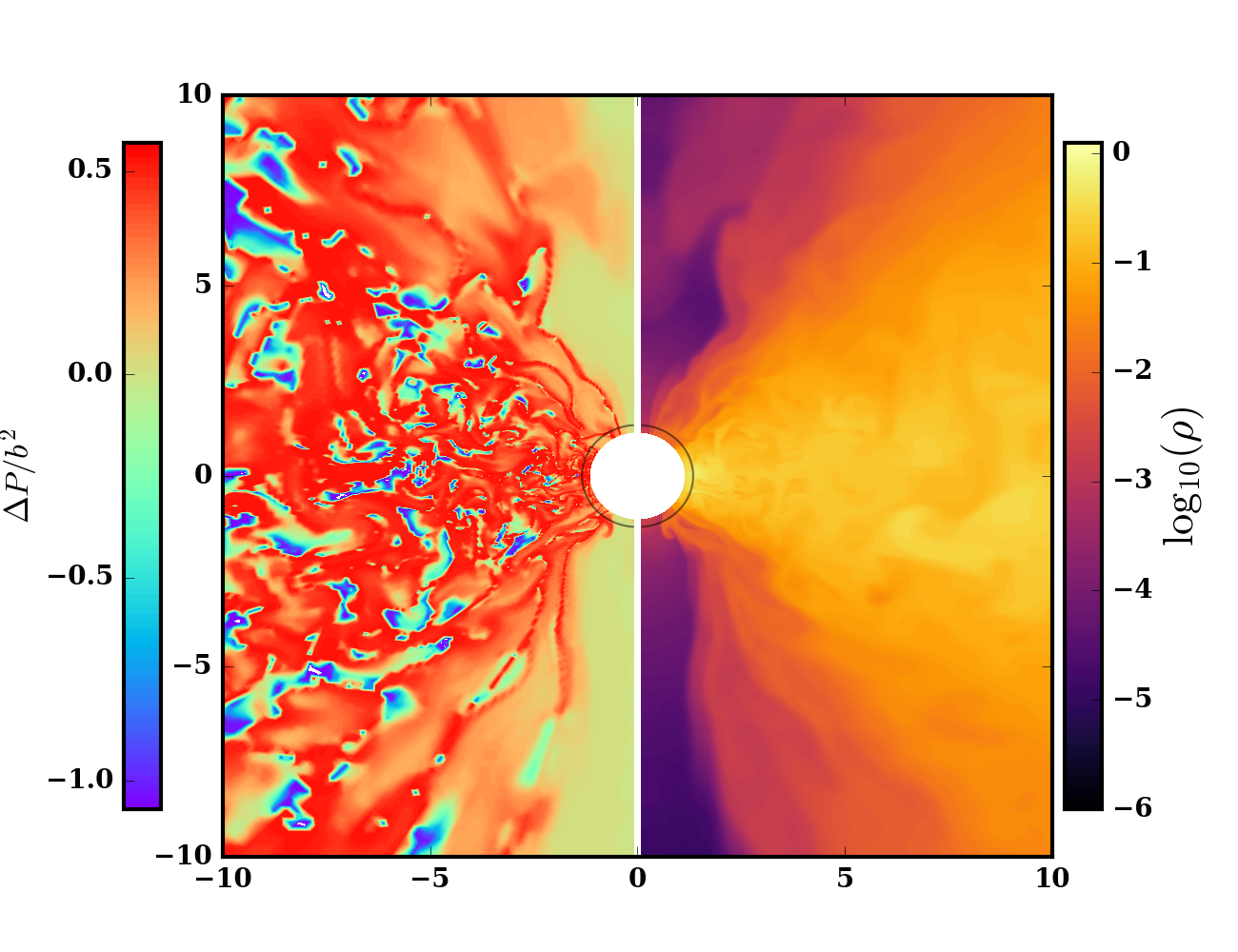
Figure 6: Vertical slice through the high-resolution EMHD model at $t=5000t_{g}$ (SANE disk). Left: Pressure anisotropy normalized by the magnetic energy density. The pressure anisotropy saturates at the threshold of the mirror instability, $\Delta P\sim b^{2}/2$, in most of the disk. Right: Fluid density, showing the magnetically driven turbulence.

In order to understand the impact of non-ideal effects on the dynamics of the disk, it is useful to look at the instantaneous and average value of the pressure anisotropy $\Delta P$. In Sec. 2, we noted that for a Keplerian velocity profile we expect the pressure anisotropy to grow to the threshold of the mirror instability, $\Delta P\approx b^{2}/2$, as long as $\beta>1$. In practice, our EMHD simulations show that this is the case even in the turbulent accretion flow resulting from the MRI-driven evolution of the disk.

To illustrate this, we show in Fig. 6 a specific realization of the pressure anisotropy $\Delta P$ for a vertical slice of the SANE disk at $t=5000t_{g}$. In most of the accretion disk (i.e. away from the magnetically dominated polar regions, where $\beta\ll 1$), we find that $\Delta P\approx b^{2}/2$, the threshold of the mirror instability. Some small portions of the disk instead find themselves at the threshold of the firehose instability, $\Delta P\approx-b^{2}$.

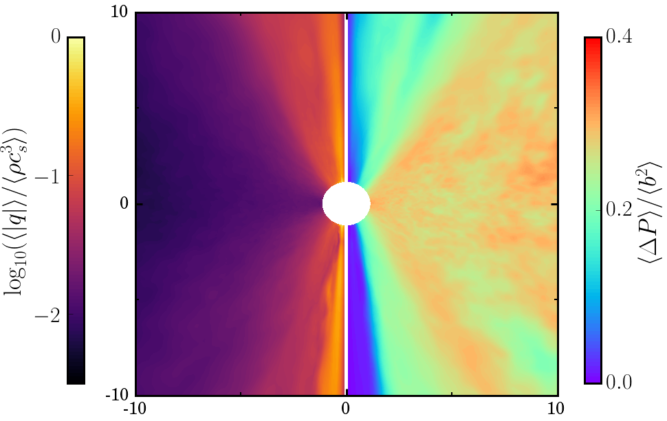
Figure 7: Time and azimuthally-averaged profiles for the high-resolution EMHD model (SANE disk). Left: Ratio of the averages of $|q|=\sqrt{q^{\mu}q_{\mu}}$ and $q_{\rm max}=\rho c_{s}^{3}$. Right: Ratio of the averages of $\Delta P$ and $b^{2}$. While the heat flux is far from saturated in the disk (typically a few percent of its saturation value), the average pressure anisotropy is of order the magnetic pressure, $\sim(0.2-0.4)b^{2}$.

The average pressure anisotropy in the disk is shown in Fig. 7. Once we average $\Delta P$ in time and over the azimuthal direction, we find that $\langle\Delta P\rangle\approx(0.2-0.4)\langle b^{2}\rangle$. This is consistent with the more detailed distributions of $\Delta P$ provided in Figs. 8-9: in steady-state, about $65\%$ of the disk mass is close to the mirror instability threshold, at $\Delta P\gtrsim 0.99\Delta P_{\rm mirror}$. About $5\%$ of the disk mass is close to the firehose instability threshold, and the average value of $\Delta P/b^{2}$ is $0.25$. In earlier axisymmetric simulations, we already noted that about half of the disk was at the threshold of the mirror instability (Foucart et al., 2016). These results show that the fluid is pushed even more towards the mirror instability threshold in 3D simulations.

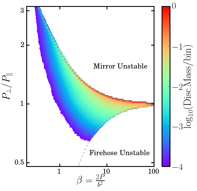
Figure 8: Mass-weighted distribution function in the $\beta$-$(P_{\perp}/P_{\parallel})$ plane (SANE disk). The dashed curve shows the threshold of the mirror instability, and the dot-dashed curve the threshold of the firehose instability. Most of the mass remains at the mirror-instability threshold. We show the total mass integrated over 100 equidistant snapshots of the simulation between $(4000-6000)GM/c^{3}$. The bins are logarithmically spaced in both dimensions, and we only include points at $r<9GM/c^{2}$, where the flow is in quasi-steady state.

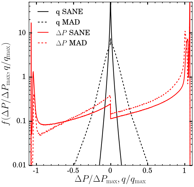
Figure 9: Mass-weighted distribution function of the normalized pressure anisotropy ($\Delta P/\Delta P_{\rm max}$, with $\Delta P_{\rm max}$ the threshold of the mirror/firehose instability for positive/negative $\Delta P$) and normalized heat flux ($q/q_{\rm max}$, with $q_{\rm max}=\rho c_{s}^{3}$) for the SANE (solid lines) and MAD (dashed lines) configurations. Most of the fluid shows a large pressure anisotropy $\Delta P\sim\Delta P_{\rm mirror}$, and a small heat flux. The discontinuity in the distribution of $\Delta P$ at $\Delta P=0$ is due to the different normalization for positive/negative $\Delta P$.

In contrast to these large pressure anisotropies, heat conduction in the disk remains negligible throughout the simulation. Fig. 7 and Fig. 9 show that the magnitude of the heat flux in the disk is, on average, only a few percent of the free-streaming value $q_{\rm max}=\rho c_{s}^{3}$. The heat flux only becomes larger in the polar regions, where magnetic fields dominate the evolution of the system. This is consistent with results obtained in axisymmetry, where the low value of the heat flux was due to (i) the saturation of the pressure anisotropy, which causes a suppression by a factor of $\beta^{-1}$ of the collision timescale $\tau_{R}$, and thus of the heat flux; and (ii) the misalignment between the poloidal temperature gradient and the largely azimuthal magnetic field. As heat conduction can only act along magnetic field lines, temperature gradients orthogonal to the magnetic field cannot drive heat conduction in the disk. Fig. 6 shows that, even in 3D, the heat flux is negligible in regions in which $\Delta P$ saturates.

From our EMHD simulation, we thus deduce that the average impact of the non-ideal effects in the compact, SANE disk studied here might be close to what one would obtain by setting $\Delta P\sim 0.25b^{2}$ and $q\sim 0$. We also note that our results critically depend on the treatment of the mirror instability in the EMHD model. We assume that when driven above the threshold of the mirror instability, $\Delta P$ saturates at nearly exactly the instability threshold $\Delta P_{\rm mirror}$, through an increase in the effective collision rate in the plasma. Our results are only physical if this approximation captures the global behavior of the plasma on length scales much larger than the Larmor radius. While current particle-in-cell simulations broadly support this model (Kunz et al., 2016), comparisons of the EMHD model with more detailed local simulations of a plasma at the mirror instability threshold will be required to test this assumption.

4.4 Stress tensor and angular momentum transport

In previous sections, we showed that the pressure anisotropy in the EMHD simulations of SANE disks is, in a time average sense, $\Delta P\sim b^{2}/4$. In Sec. 2, we also argued that the associated shear stress, $\sim-\Delta P\hat{b}^{\mu}\hat{b}^{\nu}$, is effectively of the same form as the magnetic shear stress, $-b^{2}\hat{b}^{\mu}\hat{b}^{\nu}$. As far as the shear stress is concerned, the pressure anisotropy $\Delta P$ and the magnetic energy density $b^{2}$ are interchangeable. Additionally, for $\beta\gg 1$, the magnetic energy density and isotropic magnetic pressure do not play a particularly important role in the dynamics of the accretion flow.

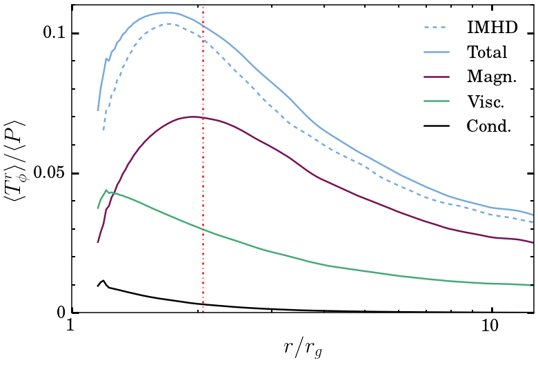
Figure 10: Average (r,$\phi$) component of the stress tensor, $\langle T^{r}_{\phi}\rangle$, normalized by the average pressure $\langle P\rangle$ in the SANE simulations. The dashed curve shows the magnetic stress in the IMHD simulation. The EMHD stress is decomposed into magnetic, viscous, and conduction components. The total stress is nearly the same in the EMHD and IMHD simulations. The lower value of the magnetic stress in the EMHD model is compensated by the viscous stress. The red dot-dashed line shows the location of the ISCO. The turnover of the magnetic stresses at the ISCO is due to the growing contribution of the advection term ($\sim b^{2}u^{r}u_{\phi}$), which is negligible at large radii, does not have a viscous counterpart, and is transporting angular momentum inwards.

Accordingly, we may expect similar steady-state accretion flows to be reached in EMHD and IMHD if $b^{2}_{\rm IMHD}=b^{2}_{\rm EMHD}+\Delta P_{\rm EMHD}\approx(5/4)b^{2}_{\rm EMHD}$. Our simulations appear consistent with this interpretation of the impact of the pressure anisotropy: in the SANE configuration, we find similar density and temperature profiles for the EMHD and IMHD models, but with a weaker magnetic field in the EMHD model, e.g. the plasma parameter $\beta$ satisfies $\beta_{\rm EMHD}=(1.2-1.4)\beta_{\rm IMHD}$.

We can have a more direct look at the component of the stress-energy tensor responsible for angular momentum transport in the disk, $T^{r}_{\phi}$. We show radial profiles of $T^{r}_{\phi}$ (averaged over time and azimuthal angle, integrated over the polar angle, and normalized by the gas pressure) in Fig. 10. The first notable result is that the total stress is nearly identical for the IMHD and EMHD simulations. However, in the IMHD model the entirety of the stress is due to the magnetic field. In the EMHD model, outside the innermost stable circular orbit of the black hole, $(70-75)\%$ of the $r-\phi$ component of the stress is due to the magnetic field and $(25-30)\%$ to the pressure anisotropy. While this fraction of the stress due to the pressure anisotropy is slightly larger than one might have expected based on the simplistic model of a constant ratio $\Delta P:b^{2}=1:4$, the properties of the stress tensor are broadly consistent with the view that in EMHD the pressure anisotropy effectively replaces a fraction of the IMHD magnetic field, with no obvious other significant effects on the dynamics of the disk.

Finally, we note that the profiles for the effective $\alpha$-viscosity (defined by $\langle T^{r}_{\phi}\rangle=\alpha\langle P\rangle$), surface density $\Sigma$, and temperature $T$ shown in Fig. 5 and Fig.10 do not agree with the usual 1D result $\alpha\Sigma\Theta/\Omega={\rm constant}$. This can be understood from the conservation of angular momentum equation (expressed, for simplicity, in the Newtonian limit and for a quasi-Keplerian thin disk),

$$\dot{M}r^{2}\Omega+2\pi\alpha r^{2}\Sigma\Theta=\dot{J},$$ (27)

with $\dot{J}$ the net angular momentum transported through the disk, which is constant in the steady state region. As an order of magnitude estimate, we should have $\dot{J}\sim\dot{M}j_{\rm ISCO}$, with $j_{\rm ISCO}$ the specific angular momentum at the ISCO, and thus $\dot{M}j(r)\sim(1-2)\dot{J}$ within the steady-state accretion flow in our simulations. The relation $\alpha\Sigma\Theta/\Omega={\rm constant}$ is only valid when $\dot{M}j(r)\gg\dot{J}$, which is typically the case at larger radii but not close to the ISCO. At small radii and outside the ISCO, we instead expect $\Sigma$ to grow as $(r-r_{\rm ISCO})$ increases, as seen in our simulations.

5 MAD Results

The magnetically arrested disk (MAD) simulations provide us with a different regime to study the impact of non-ideal effects. The MAD simulations are initialized using a wider torus in which we seed a single loop of poloidal magnetic field (see Sec. 3.1). The vertical magnetic flux crossing the equatorial plane inside of the pressure maximum of the disk is significantly larger in the MAD configuration than in the SANE configuration. This vertical flux is slowly accreted onto the black hole, up to the point at which the magnetic flux threading the black hole becomes large enough to vertically compress the disk and obstruct the gas infall. This happens when the magnetic pressure from the jet is in equilibrium with the ram pressure of the infalling gas. The accretion flow close to the horizon then proceeds through a very thin disk. That disk is more strongly magnetized than in the SANE case ($\beta\sim 1$ at the ISCO), and the magnetic pressure of the jet plays an important role in its evolution. With a dynamically important magnetic pressure, we expect larger differences between the magnetic and viscous stresses than in the SANE disk. However, we will see that this does not translate into significant differences between the EMHD and IMHD results. Accordingly, we will not repeat here the full analysis of the accretion flow provided for the SANE case, and will instead only discuss the main differences between the MAD and SANE results.

In order to determine when we enter the MAD state, we monitor the normalized flux across the horizon,

$$\phi_{\rm BH}=\sqrt{4\pi}\frac{\oint|B^{a}|\sqrt{-g}dS}{2\dot{M}^{1/2}},$$ (28)

with the surface integral taken on the event horizon of the black hole, $a=\log{(r)}$, and $g$ the determinant of the metric $g_{\mu\nu}$ in the coordinates $(t,a,b,c)$ of the numerical grid (see Sec. 3.3). $\phi_{\rm BH}$ grows steadily up to $t\sim(5-6)10^{3}t_{g}$, then oscillates around the average value $\bar{\phi}_{\rm BH}=75$ in EMHD, and $\bar{\phi}_{\rm BH}=74$ in IMHD for times $t>6000t_{g}$.  This is comparable to the value measured for the same black hole spin in Tchekhovskoy et al. (2012) ($\bar{\phi}_{\rm BH}=60$). The difference between our results and Tchekhovskoy et al. (2012) is most likely due to the use of a different equation of state, resulting in a thicker disk in this work. We note that the remarkable agreement in $\phi_{\rm BH}$ between the IMHD and EMHD simulations occurs despite the accretion rate being $20\%$ lower for the EMHD model.

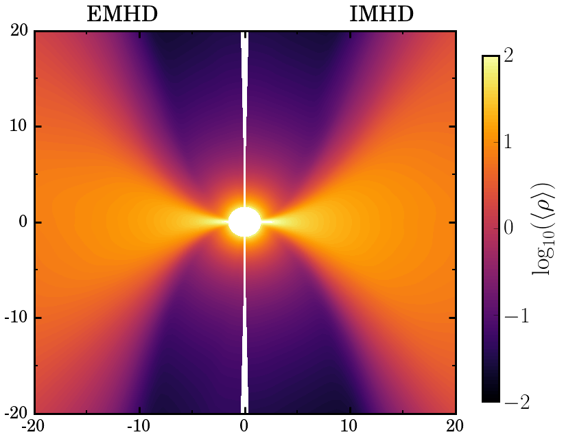
Figure 11: Density of the MAD accretion flow in the EMHD (left) and IMHD (right) models, averaged over the azimuthal direction and within the time window $t=(6000-14000)t_{g}$. A magnetically arrested accretion flow is observed in both models.

In the rest of this section, we focus on the time interval $t=(6-14)10^{3}t_{g}$ during which the simulations are in the MAD state, and compute time-averaged quantities over that interval. Time-averaged density profiles of the steady-state accretion flow are shown in Fig. 11 for the EMHD and IMHD models. Both simulations clearly show a vertically compressed accretion flow, indicative of the MAD state (Tchekhovskoy et al., 2011), instead of the thick accretion flow observed in the SANE configuration. The EMHD and IMHD results are very similar. While we did not find any steady-state disk outflows in the SANE configuration, a clear inflow-outflow structure appears in the MAD simulations, as shown in Fig. 12. The inflowing fluid covers the region within $\sim 40^{\circ}$ of the equatorial plane, while outflows are present at higher latitudes. The magnetically dominated jet itself covers the region $10^{\circ}-20^{\circ}$ away from the poles. The net average mass flow across spheres of fixed radii is constant up to $r\sim 50r_{g}$. The MAD disk has a larger steady-state region than the SANE disk due to efficient angular momentum transport by large scale magnetic stresses (see Fig. 13, and discussion below).

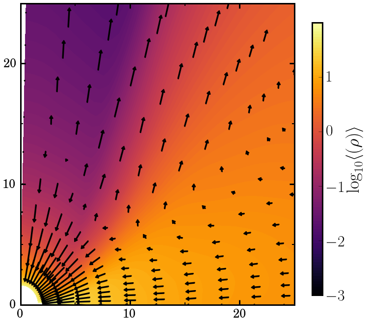
Figure 12: Density and velocity of the MAD accretion flow in the EMHD model, averaged over the azimuthal direction and within the time window $t=(6000-14000)t_{g}$. As opposed to the SANE model, we observe a clear inflow-outflow structure in the accretion flow.

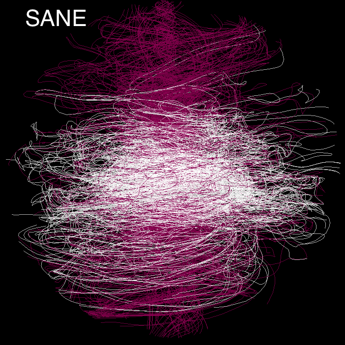
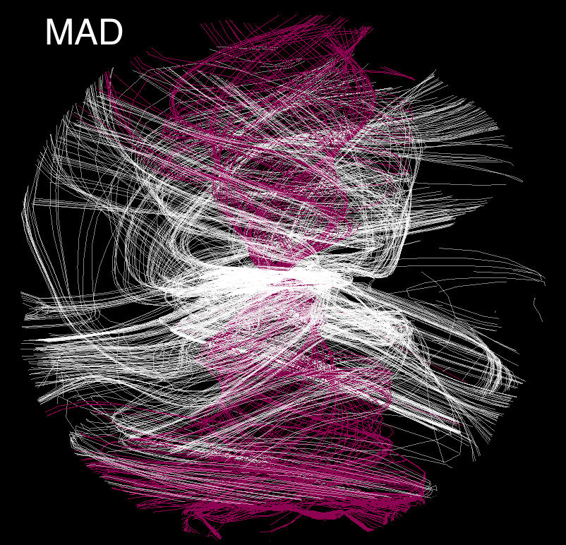
Figure 13: Magnetic streamlines for the SANE (top) and MAD (bottom) simulations, using the EMHD model. White streamlines are seeded in the equatorial plane, while purple streamlines are seeded above and below that plane (at $z=\pm 10r_{g}$ for SANE, $z=\pm 20r_{g}$ for MAD). In all cases, the streamlines are randomly seeded within a rectangular region centered on the polar axis in which the disk is in steady state [squares of size $(10r_{g})^{2}$ for the SANE simulation and $(20r_{g})^{2}$ for the MAD simulation]. We stop integration of the streamlines at a distance of $50r_{g}$ from the black hole. The magnetic field is more structured in the MAD simulation, with clear wind and jet regions.

Fig. 14 shows one-dimensional profiles of the accretion flow for the surface density, plasma $\beta$-parameter, and fluid temperature. In the SANE disks, the sole difference between EMHD and IMHD results was in the profile of $\beta$: the disk was more strongly magnetized in the IMHD model than in EMHD. In the MAD disks, $\beta$ and $\Sigma$ both show deviations of $15\%-25\%$, with the lower surface density being consistent with the $20\%$ slower accretion rate measured for the EMHD model. The temperature does not change by more than $10\%$ between the two models.

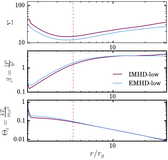
Figure 14: Same as Fig. 5, but for the MAD configuration and with time averages taken over the $t=(6000-14000)t_{g}$ interval.

Finally, Fig. 9 shows the pressure anisotropy and heat flux in the EMHD simulation. As in the SANE simulations, the pressure anisotropy $\Delta P$ saturates at the threshold of the mirror instability. The heat flux is larger for MAD disks than SANE disks, of the order of $10\%$ of its free-streaming value in large regions of the disk. This can be attributed to the higher magnetization of the MAD disk. As discussed in Sec. 2, we expect an effective collision timescale $\tau_{R}=\tau_{d}/\beta$ in the disk, which causes a suppression of the heat flux by a factor of $\beta$. While in the SANE disk we have $\beta\sim 5-15$, here we have $\beta\sim 1-3$ outside of the ISCO. The heat flux in the MAD disks is thus larger, yet remains far from the free-streaming value nearly everywhere.

As in the SANE disk, the pressure anisotropy contributes to outward angular momentum transport in the disk, with the vertically averaged shear stress satisfying $\langle T^{r}_{\phi,{\rm vis}}\rangle\sim 0.04\langle P\rangle$. Near the equatorial plane, the magnetic shear stress $T^{r}_{\phi,{\rm mag}}\sim(0.10-0.15)P$, so that the viscous shear stress is still $\sim 1/3$ of the magnetic shear stress, as in the SANE simulation. However, in the MAD configuration, there is a net extraction of angular momentum from the black hole, and most of that angular momentum is carried outward in the wind and, even more, in the jet. In these magnetically dominated regions, $\Delta P\sim P\ll b^{2}$. Accordingly, we find that the contribution of magnetic fields to angular momentum transport is $\sim 5-10$ times larger than the contribution of the pressure anisotropy in most of the steady-state region. In addition, the mass and angular momentum outflows, as well as $T^{r}_{\phi,{\rm mag}}$, are similar in the EMHD and IMHD simulations.

Overall, we thus find that the EMHD and IMHD results are very similar for the MAD disk. While the viscous shear stress due to the pressure anisotropy is larger for the MAD configuration than for the SANE configuration, the transport of angular momentum in the jet and winds due to the magnetic field dominates over the viscous shear stress.

6 Conclusions

We have presented the first global, 3D simulations including the two non-ideal effects most likely to impact the dynamics of accretion disks around slowly accreting supermassive black holes: heat conduction along magnetic field lines, and an anisotropy between the pressure parallel and perpendicular to the magnetic field direction. The latter is equivalent to an anisotropic viscosity. We start from well-known configurations for an accretion torus in hydrostatic equilibrium, which allows us to generate steady-state accretion flows in the region close to the black hole. We consider two initial configurations. The first leads to a steady-state accretion driven by magnetically-driven turbulence and viscous stresses, with the turbulence driven by the growth of the magnetorotational instability. Angular momentum transport in the disk is due to both the magnetic stress and the pressure anisotropy. The initial magnetic field has a relatively small net vertical magnetic flux, so that no significant magnetized jet forms along the black hole rotation axis. The disk remains in the so-called SANE configuration, with a plasma parameter $\beta\sim 5-15$. In the second configuration, we consider a wider initial torus with a larger net vertical magnetic flux. As the magnetic flux across the black hole horizon increases, the magnetic pressure of the jet balances the ram pressure of the accreting gas, forming a magnetically arrested disk (MAD). Angular momentum transport is now mainly due to the jet and disk winds, and the disk itself is more strongly magnetized ($\beta\sim 1-3$).

In both cases, we find that the pressure anisotropy grows rapidly, up to the point at which it should be limited by the onset of plasma instabilities (mainly the mirror instability). At this point, our EMHD model assumes that the pressure anisotropy saturates at the mirror instability threshold, with $\Delta P\approx b^{2}/2$ (for $\beta\gg 1$). Despite this large pressure anisotropy, the dynamics of the disk remains very similar in the IMHD and EMHD models. In the SANE configuration, the only difference appears to be a stronger magnetization of the disk in the IMHD simulation (by $\sim 30\%$). In the MAD configuration, there are variations of up to $25\%$ in the magnetization of the disk, with only the inner disk being more strongly magnetized in IMHD. In both cases, the temperature of the disk does not significantly depend on the chosen plasma model, with the ion temperature $\Theta$ consistent with the transformation of potential energy into thermal energy expected in a radiatively inefficient accretion disk. The ratio of the surface density to the accretion rate is also nearly the same in EMHD and IMHD. In our simulations, the heat flux remains negligible at all times.

In the SANE configuration, we argue that the agreement between the EMHD and IMHD results is largely due to the similarities between the shear stresses associated with the magnetic field and pressure anisotropy. In particular, the shear stress due to pressure anisotropy is identical to the shear stress produced by the magnetic field with the transformation $\Delta P\rightarrow b^{2}$ (see Eqs. 19-20). Thus, if $\Delta P\sim b^{2}/2$ due to the mirror instability, the impact of the viscous shear stress on the disk dynamics is very similar to that of the B-field. Practically, we propose that in the innermost regions of a SANE disk, the EMHD results can be derived, in a time-averaged sense at least, from ideal MHD results through the simple transformation

$$b^{2}_{\rm EMHD} = (0.7-0.8)b^{2}_{\rm IMHD}$$ (29)

$$\Delta P_{\rm EMHD} = (0.2-0.3)b^{2}_{\rm IMHD}.$$ (30)

Under that transformation, the evolution equations of the EMHD system are identical to the equations of ideal MHD, up to small corrections of the order of the magnetic pressure in the energy density and pressure of the fluid.

We note, however, that this argument is only valid under the restrictive condition that $\beta\gg 1$. Accordingly, that rescaling is no longer valid in the MAD configuration. When $\beta\lesssim 1$, we have $\Delta P\sim P\lesssim b^{2}/2$. The ratio of the pressure anisotropy to the gas pressure is larger than in the SANE case, but the ratio of the pressure anisotropy to the magnetic pressure is smaller than in the SANE case. The larger value of $\Delta P/P$ in MAD disks, combined with the qualitative differences between the viscous and magnetic stresses in the presence of a non-negligible magnetic pressure, could lead us to believe that non-ideal effects are more important in MAD disks than in SANE disks. However, in the MAD configuration, the magnetic stresses and pressure dominate over the gas and viscous stresses, thus reducing the impact of the pressure anisotropy on the dynamics of the disk. In the end, we find that the second effect is more important, and that there is very little difference between EMHD and IMHD MAD disks precisely because the flow dynamics is magnetically dominated ($\beta\leq 1$).

6.1 Future directions

The similarities between EMHD and IMHD simulations shown here are a strong indication that accretion disk models neglecting non-ideal effects in the dynamics of the ions are likely reasonable even for slowly accreting black holes in which the accretion flow is a nearly collisionless plasma. It is, however, important to carefully consider the limitations of this study. First, all disks studied in this work are relatively compact, and even in the MAD configuration we cannot follow the production of truly unbound outflows in the disk. The impact of non-ideal effects on disk outflows remains uncertain. In addition, heat-flow driven instabilities such as the magnetothermal instability (Balbus, 2000, MTI) may be active at larger radii in the disk (e.g. Sharma et al. 2008). The growth timescale of the MTI at small radii is likely slower than the accretion timescale, and thus the MTI cannot develop in our simulations.

Another important difference between EMHD and IMHD SANE disks is that, in the EMHD simulations, about a third of the accretion power is directly thermalized through the viscous shear stress due to the pressure anisotropy, instead of through dissipation on small scales at the end of the turbulent cascade driven by the MRI. In our simulations, this does not appreciably change the ion temperature. However, the different heating mechanisms may very well lead to different ion distribution functions. In addition, the presence of both viscous and turbulent heating might affect the relative heating of ions and electrons (e.g. Sharma et al. 2007). In this work, we solely focus on the dynamics of the disk, which is driven by the ions. But modeling the plasma as a single temperature fluid is not sufficient when constructing models for the electromagnetic emission from the disk (Ressler et al., 2017; Sadowski et al., 2017).

It is also critical to reiterate that the EMHD model used here is itself an approximation of the complex plasma physics occurring in these disks. In our calculations, the effects of the mirror instability are particularly important. The validity of our fluid sub-grid model for collisionless plasmas close to the mirror instability threshold is an active area of research (e.g., Kunz et al. 2016). It is quite possible that surprises will arise that will impact the understanding of sub-Eddington disk dynamics.

Finally, there are interesting outstanding questions about the connection between our global results and shearing box studies of the growth and saturation of the MRI. The latter indicate that the saturation of the MRI is sensitive to the inclusion of explicit (rather than numerical) viscosity and resistivity, and their ratio, the magnetic Prandtl number (Lesur & Longaretti, 2007; Fromang et al., 2007). In our IMHD simulations, both viscosity and resistivity are set by numerical dissipation. The numerical viscosity and resistivity both decrease with resolution, but numerical simulations in ideal MHD have shown that the numerical magnetic Prandtl number is largely independent of the numerical resolution (Guan & Gammie, 2009; Lesur & Longaretti, 2009; Fromang & Stone, 2009), so that effectively all global simulations of accretion disks in ideal MHD are performed at constant turbulent Prandtl number. On the other hand, the EMHD model introduces a new explicit source of viscosity, which is larger than the numerical viscosity. Should we then expect the MRI to saturate at a very different level in EMHD and IMHD because the former effectively has a larger (albeit anisotropric) microphysical magnetic Prandtl number? If so, how is this consistent with our results which show very little difference between EMHD and IMHD? Shearing-box simulations with an anisotropic viscosity and an explicit magnetic resistivity may help shed some light on this issue. It may be that including an explicit isotropic viscosity small compared to the anisotropic viscosity is also important in EMHD simulations.

Appendix A Coordinate transformation

An important disadvantage of the spherical polar coordinates commonly used when simulating accretion onto black holes is that the minimum grid spacing scales quadratically with resolution, i.e. if the number of grid points along each dimension is multiplied by $n$, the minimum grid spacing is divided by $n^{2}$. This is due to the aximuthal grid spacing of the points closest to the polar axis, which scales as $\Delta x_{\rm min}\propto r\times\Delta\theta\times\Delta\phi$. As the maximum time step for stable evolution is proportional to the minimum grid spacing, the cost of 3-dimensional simulations scales like $n^{5}$.

One way to avoid this issue and recover the same $n^{4}$ scaling as for cartesian grids is to use mesh refinement and decrease the number of cells in the azimuthal direction when close to the polar axis. In our simulations, we instead use coordinate transformations to decrease the resolution along $\theta$ close to the polar axis. While our method leads to more distorted grid cells close to the polar axis, it has the advantage of avoiding the many complications associated with the use of mesh refinement.

Sec. 3.3 describes the structure of our numerical grid and the main coordinate transformations used in our simulations. We define a map between the coordinates of our numerical grid $(t,a,b,c)$ and the usual Kerr-Schild coordinates $(t,r,\theta,\phi)$ through Eqs. (21-26), plus a map $\tilde{\theta}\rightarrow\theta$ described below. Eqs. (21-26) focus resolution close to the black hole, thanks to the exponential radial map. They also force the use of a map uniform in $\tilde{\theta}$ close to the horizon of the black hole, while focusing points in the equatorial regions at larger radii. A uniform map at small radii is useful to maximize the minimum grid spacing in the $\theta$ direction, while focusing points in the equatorial regions provides resolution where it is most needed to capture the fastest growing mode of the MRI.

The map $\tilde{\theta}\rightarrow\theta$ is used to avoid small azimuthal grid spacings at small cylindrical radii near the poles and follows the approach developed by Tchekhovskoy et al. (2011). For completeness, we give the details here. Broadly speaking, this approach transforms the spherical polar coordinates into nearly cylindrical coordinates in a small region within a radius $r_{\rm cyl}$ of the black hole center and a distance $\rho_{\rm cyl}\sim r_{\rm cyl}\theta_{\rm cyl}$ of the polar axis. More precisely, for $0\leq\theta\leq\pi/2$, the map is defined as

$$\sin(\theta)=S_{\rm max}\left(\sin(\tilde{\theta}),f_{2}(r,\tilde{\theta}),\frac{r_{\rm cyl}+r_{\rm in}}{2r}df\right),$$ (31)

with $r_{\rm in}$ the radius of the inner boundary.

The function $S_{\rm max}$ is defined as

$$S_{\rm max}(x_{0},x_{1},dx)=x_{1}-dxF\left(\frac{x_{1}-x_{0}}{dx}\right),$$ (32)

with $F(x)=0$ for $x<-1$, $F(x)=x$ for $x>1$, and

$$2F(x) = x+1+\frac{1}{160\pi}\sin\left(\frac{5\pi(x+1)}{2}\right)+\frac{5}{96\pi}\sin\left(\frac{3\pi(x+1)}{2}\right)$$ (33)

$$-\frac{35}{16\pi}\sin\left(\frac{\pi(x+1)}{2}\right)$$

for $-1\leq x\leq 1$. Practically, $S_{\rm max}$ returns the maximum of $(x_{0},x_{1})$ if $x_{0}\gg x_{1}$ or $x_{0}\ll x_{1}$, and smoothly transitions between $x_{0}$ and $x_{1}$ when $x_{0}\sim x_{1}$. Eq. 31 is thus a smooth transition between $\theta=\tilde{\theta}$ and $\sin(\theta)=f_{2}(r,\tilde{\theta})$. The latter is the ‘cylindrified’ coordinate, defined as

$$f_{2}(r,\tilde{\theta})=S\left(\frac{r_{\rm cyl}}{r}\sin(\tilde{\theta}),\sin\left(\theta_{2}(r,\tilde{\theta})\right),|\sin{(\theta_{2}(r,0)})|,r-r_{\rm cyl}\right),$$ (34)

where $S(x_{0},x_{1},dx,A)=S_{\rm max}(x_{0},x_{1},dx)$ if $A>0$ and $S(x_{0},x_{1},dx,A)=-S_{\rm max}(-x_{0},-x_{1},dx)$ for $A<0$. The angle $\theta_{2}$ is

$$\theta_{2}(r,\tilde{\theta}) = \theta_{1}(r)+\left(\pi/2-\theta_{1}(r)\right)\frac{\tilde{\theta}-\theta_{\rm cyl}}{\pi/2-\theta_{\rm cyl}},$$ (35)

$$\sin{\left(\theta_{1}(r)\right)} = \frac{r_{\rm cyl}}{r}\sin{(\theta_{\rm cyl})}.$$ (36)

In the limit $\sin(\theta)=f_{2}=\frac{r_{\rm cyl}}{r}\sin{(\tilde{\theta})}$, lines of constant $\tilde{\theta}$ are vertical lines at a constant distance $\rho=r_{\rm cyl}\sin{(\tilde{\theta})}$ from the polar axis. The smoothing functions are chosen so that $f_{2}\approx\sin{\tilde{\theta}}$ for $\tilde{\theta}\gg\theta_{\rm cyl}$, while $f_{2}\approx\frac{r_{\rm cyl}}{r}\sin{(\tilde{\theta})}$ for $\tilde{\theta}\lesssim\theta_{\rm cyl}$.

The smoothing width $\frac{r_{\rm cyl}+r_{\rm in}}{2r}df$, on the other hand, provides the transition between ‘cylindrified’ coordinates $f_{2}$ and ‘standard’ coordinates $\sin{(\tilde{\theta})}$ around $r\sim r_{\rm cyl}$. We use

$$df=|f_{2}(\frac{r_{\rm cyl}+r_{\rm in}}{2},\tilde{\theta})-\sin{(\tilde{\theta})}|.$$ (37)

In practice, we choose $\theta_{\rm cyl}\sim\pi/N_{\theta}$, with $N_{\theta}$ the number of grid cells in the polar direction. The map $\tilde{\theta}\rightarrow\theta$ thus only affects the grid cells closest to the polar axis. The parameter $r_{\rm cyl}$ is resolution dependent, and chosen to maximize the smallest grid spacing in our computational domain (we use $r_{\rm cyl}=8r_{\rm in}$ in the high-resolution simulations of SANE disks presented in this work). The map for $\pi/2<\theta\leq\pi$ is obtained by requiring symmetry across the equatorial plane.

References

- Balbus (2000) Balbus S. A., 2000, ApJ, 534, 420
- Balbus (2004) Balbus S. A., 2004, ApJ, 616, 857
- Balbus & Hawley (1991) Balbus S. A., Hawley J. F., 1991, ApJ, 376, 214
- Bisnovatyi-Kogan & Ruzmaikin (1974) Bisnovatyi-Kogan G. S., Ruzmaikin A. A., 1974, Ap&SS, 28, 45
- Bisnovatyi-Kogan & Ruzmaikin (1976) Bisnovatyi-Kogan G. S., Ruzmaikin A. A., 1976, Ap&SS, 42, 401
- Braginskii (1965) Braginskii S. I., 1965, Reviews of Plasma Physics, 1, 205
- Chandra et al. (2015) Chandra M., Gammie C. F., Foucart F., Quataert E., 2015, ApJ, 810, 162
- Chandra et al. (2017) Chandra M., Foucart F., Gammie C. F., 2017, ApJ, 837, 92
- Colella & Woodward (1984) Colella P., Woodward P. R., 1984, J.~Chem.~Phys., 54, 174
- De Villiers et al. (2003) De Villiers J.-P., Hawley J. F., Krolik J. H., 2003, ApJ, 599, 1238
- Doeleman et al. (2009) Doeleman S., et al., 2009, in astro2010: The Astronomy and Astrophysics Decadal Survey. p. 68 (arXiv:0906.3899)
- Eisenhauer et al. (2008) Eisenhauer F., et al., 2008, in Optical and Infrared Interferometry. p. 70132A (arXiv:0808.0063), doi:10.1117/12.788407
- Fishbone & Moncrief (1976) Fishbone L. G., Moncrief V., 1976, ApJ, 207, 962
- Foucart et al. (2016) Foucart F., Chandra M., Gammie C. F., Quataert E., 2016, MNRAS, 456, 1332
- Fromang & Stone (2009) Fromang S., Stone J. M., 2009, A&A, 507, 19
- Fromang et al. (2007) Fromang S., Papaloizou J., Lesur G., Heinemann T., 2007, A&A, 476, 1123
- Gammie et al. (2003) Gammie C. F., McKinney J. C., Tóth G., 2003, ApJ, 589, 444
- Ghisellini et al. (2014) Ghisellini G., Tavecchio F., Maraschi L., Celotti A., Sbarrato T., 2014, Nature, 515, 376
- Guan & Gammie (2009) Guan X., Gammie C. F., 2009, ApJ, 697, 1901
- Hellinger et al. (2006) Hellinger P., Trávníček P., Kasper J. C., Lazarus A. J., 2006, Geophys. Res. Lett., 33, 9101
- Ho (2009) Ho L. C., 2009, ApJ, 699, 626
- Igumenshchev (2008) Igumenshchev I. V., 2008, ApJ, 677, 317
- Igumenshchev et al. (2003) Igumenshchev I. V., Narayan R., Abramowicz M. A., 2003, ApJ, 592, 1042
- Kasper et al. (2002) Kasper J. C., Lazarus A. J., Gary S. P., 2002, Geophysical Research Letters, 29, 20
- Koide et al. (1999) Koide S., Shibata K., Kudoh T., 1999, ApJ, 522, 727
- Kunz et al. (2014) Kunz M. W., Schekochihin A. A., Stone J. M., 2014, Physical Review Letters, 112, 205003
- Kunz et al. (2016) Kunz M. W., Stone J. M., Quataert E., 2016, Physical Review Letters, 117, 235101
- Lesur & Longaretti (2007) Lesur G., Longaretti P.-Y., 2007, MNRAS, 378, 1471
- Lesur & Longaretti (2009) Lesur G., Longaretti P.-Y., 2009, A&A, 504, 309
- McKinney & Gammie (2004) McKinney J. C., Gammie C. F., 2004, ApJ, 611, 977
- Narayan et al. (2003) Narayan R., Igumenshchev I. V., Abramowicz M. A., 2003, PASJ, 55, L69
- Narayan et al. (2012) Narayan R., SÄ dowski A., Penna R. F., Kulkarni A. K., 2012, MNRAS, 426, 3241
- Quataert et al. (2002) Quataert E., Dorland W., Hammett G. W., 2002, ApJ, 577, 524
- Ressler et al. (2017) Ressler S. M., Tchekhovskoy A., Quataert E., Gammie C. F., 2017, MNRAS, 467, 3604
- Riquelme et al. (2015) Riquelme M. A., Quataert E., Verscharen D., 2015, ApJ, 800, 27
- Sadowski et al. (2017) Sadowski A., Wielgus M., Narayan R., Abarca D., McKinney J. C., Chael A., 2017, MNRAS, 466, 705
- Sharma et al. (2007) Sharma P., Quataert E., Hammett G. W., Stone J. M., 2007, ApJ, 667, 714
- Sharma et al. (2008) Sharma P., Quataert E., Stone J. M., 2008, MNRAS, 389, 1815
- Shiokawa et al. (2012) Shiokawa H., Dolence J. C., Gammie C. F., Noble S. C., 2012, ApJ, 744, 187
- Sironi & Narayan (2015) Sironi L., Narayan R., 2015, ApJ, 800, 88
- Tchekhovskoy & Giannios (2015) Tchekhovskoy A., Giannios D., 2015, MNRAS, 447, 327
- Tchekhovskoy & McKinney (2012) Tchekhovskoy A., McKinney J. C., 2012, MNRAS, 423, L55
- Tchekhovskoy et al. (2011) Tchekhovskoy A., Narayan R., McKinney J. C., 2011, MNRAS, 418, L79
- Tchekhovskoy et al. (2012) Tchekhovskoy A., McKinney J. C., Narayan R., 2012, in Journal of Physics Conference Series. p. 012040 (arXiv:1202.2864), doi:10.1088/1742-6596/372/1/012040
- Tchekhovskoy et al. (2014) Tchekhovskoy A., Metzger B. D., Giannios D., Kelley L. Z., 2014, MNRAS, 437, 2744
- Yuan & Narayan (2014) Yuan F., Narayan R., 2014, ARA&A, 52, 529
- Zamaninasab et al. (2014) Zamaninasab M., Clausen-Brown E., Savolainen T., Tchekhovskoy A., 2014, Nature, 510, 126