The spectrum of a vertex model and related spin one chain sitting in a genus five curve.
M.J. Martins

Universidade Federal de São Carlos
Departamento de Física
C.P. 676, 13565-905, São Carlos (SP), Brazil

We derive the transfer matrix eigenvalues of a three-state vertex model whose weights are based on a $\mathrm{R}$-matrix not of difference form with spectral parameters lying on a genus five curve. We have shown that the basic building blocks for both the transfer matrix eigenvalues and Bethe equations can be expressed in terms of meromorphic functions on an elliptic curve. We discuss the properties of an underlying spin one chain originated from a particular choice of the $\mathrm{R}$-matrix second spectral parameter. We present numerical and analytical evidences that the respective low-energy excitations can be gapped or massless depending on the strength of the interaction coupling. In the massive phase we provide analytical and numerical evidences in favor of an exact expression for the lowest energy gap. We point out that the critical point separating these two distinct physical regimes coincides with the one in which the weights geometry degenerate into union of genus one curves.

Keywords: spin one chain, vertex model, high genus curve.

June 2017

1 Introduction

The $\mathrm{R}$-matrix is one of the basic elements in the theory of classical two-dimensional integrable vertex model of statistical mechanics. In general, it is a numerical matrix of size $N^{2}\times N^{2}$ depending on two independent spectral parameters $\lambda$ and $\mu$ denoted here by $\mathrm{R}(\lambda,\mu)\in\mathbb{C}^{N}\otimes\mathbb{C}^{N}$. The integer $N$ is related to the number of possible statistical configurations at the edges of the vertex model. For integrability it is sufficient to impose that the $\mathrm{R}$-matrix fulfill the Yang-Baxter equation [1],

$$\mathrm{R}_{12}(\lambda_{1},\lambda_{2})\mathrm{R}_{13}(\lambda_{1},\lambda_{3})\mathrm{R}_{23}(\lambda_{2},\lambda_{3})=\mathrm{R}_{23}(\lambda_{2},\lambda_{3})\mathrm{R}_{13}(\lambda_{1},\lambda_{3})\mathrm{R}_{12}(\lambda_{1},\lambda_{2}),$$ (1)

where $\mathrm{R}_{ab}(\lambda_{a},\lambda_{b})\in\mathbb{C}^{N}\otimes\mathbb{C}^{N}\otimes\mathbb{C}^{N}$ acts as the matrix $\mathrm{R}(\lambda_{a},\lambda_{b})$ on the $a$-th and $b$-th subspaces and as the identity on the remaining subspace component.

From a given $\mathrm{R}$-matrix one can always build an integrable vertex model interpreting the matrices elements as the Boltzmann weights attached to the four edges of a vertex. The respective row-to-row transfer matrix on a square lattice of size $\mathrm{L}\times\mathrm{L}$ can formally be written as an ordered product of $\mathrm{R}$-matrices [2],namely

$$\mathrm{T}(\lambda)=\mathrm{Tr}_{0}\left[\mathrm{R}_{01}(\lambda,\mu)\mathrm{R}_{02}(\lambda,\mu)\dots\mathrm{R}_{0\mathrm{L}}(\lambda,\mu)\right],$$ (2)

where the symbol $0$ denotes the auxiliary space associated to the horizontal degrees of freedom. The trace is taken on such space and the second spectral parameter $\mu$ plays the role of an additional coupling of the model.

This vertex model generates a family of local Hamiltonians once we consider that the $\mathrm{R}$-matrix is regular at some point $\lambda_{0}$. This is to say that $\mathrm{R}(\lambda_{0},\mu)$ is proportional to the permutator $\mathrm{P}=\sum_{a,b=1}^{N}e_{ab}\otimes e_{ba}$ where $e_{ab}$ are the $N\times N$ Weyl matrices. It follows that the logarithmic expansion of the transfer matrix (2) around the point $\lambda_{0}$ generates a sequence of local commuting operators [3, 4] and the Hamiltonian is the first non-trivial charge,

$$\mathrm{H}=\sum_{j=1}^{\mathrm{L}}\mathrm{P}_{j,j+1}\frac{\partial}{\partial\lambda}\mathrm{R}_{j,j+1}(\lambda,\mu)|_{\lambda=\lambda_{0}},$$ (3)

where periodic boundary condition is assumed.

The physical understanding of vertex models needs the diagonalization of their transfer matrices which are able to provide us the free energy and the nature of the low-energy excitations. The majority of the results on that matter has been concentrated in the particular situation of $\mathrm{R}$-matrices depending on the difference of the spectral variables. The exact diagonalization of the transfer matrix of vertex models whose $\mathrm{R}$-matrices are not of difference form are in fact more rare. As a notable exception one could mention is the covering vertex model associated to the one-dimensional Hubbard Hamiltonian [5, 6]. The purpose of this paper is to expand the number of examples in the literature dealing with the spectrum of transfer matrices based on non-additive $\mathrm{R}$-matrices. To this end we will investigate the structure of the transfer matrix eigenvalues of a three-state vertex model with weights lying on a genus five curve proposed recently by the author [7]. More specifically, we shall consider the Yang-Baxter solution denominated in [7] special branch case whose underlying curve $\mathrm{C}$ has the following affine form,

$$\mathrm{C}=(x^{2}+\frac{y^{2}}{\varepsilon})(x^{2}+\varepsilon y^{2})^{2}+\mathrm{U}\sqrt{\varepsilon}xy(x^{2}+\varepsilon y^{2})-x^{2}+y^{2}=0,$$ (4)

where $x$ and $y$ are the curve affine variables, the parameter $\mathrm{U}$ is free while $\varepsilon=\exp(\pm\mathbf{\imath}\pi/3)$. The basic structure of the $\mathrm{R}$-matrix up to an overall normalization is given by,

$$\scriptsize{\mathrm{R}(\lambda_{1},\lambda_{2})=\left[\begin{array}[]{ccc|ccc|ccc}{a}(\lambda_{1},\lambda_{2})&0&0&0&0&0&0&0&0\\ 0&{b}(\lambda_{1},\lambda_{2})&0&1&0&0&0&0&0\\ 0&0&{f}(\lambda_{1},\lambda_{2})&0&{d}(\lambda_{1},\lambda_{2})&0&{h}(\lambda_{1},\lambda_{2})&0&0\\ \hline\cr 0&1&0&\overline{b}(\lambda_{1},\lambda_{2})&0&0&0&0&0\\ 0&0&\varepsilon{d}(\lambda_{1},\lambda_{2})&0&{g}(\lambda_{1},\lambda_{2})&0&{d}(\lambda_{1},\lambda_{2})&0&0\\ 0&0&0&0&0&\overline{b}(\lambda_{1},\lambda_{2})&0&1&0\\ \hline\cr 0&0&\overline{h}(\lambda_{1},\lambda_{2})&0&\varepsilon{d}(\lambda_{1},\lambda_{2})&0&{f}(\lambda_{1},\lambda_{2})&0&0\\ 0&0&0&0&0&1&0&{b}(\lambda_{1},\lambda_{2})&0\\ 0&0&0&0&0&0&0&0&{a}(\lambda_{1},\lambda_{2})\\ \end{array}\right].}$$ (5)

For the purposes of this paper we have performed a number of simplifications on the expressions of the $\mathrm{R}$-matrix elements originally presented in [7]. It turns out that they can be rewritten as follows,

$$a(\lambda_{1},\lambda_{2})=\frac{x_{1}x_{2}}{x_{2}^{2}+\varepsilon y_{2}^{2}}+\varepsilon\frac{y_{1}y_{2}}{x_{1}^{2}+\varepsilon y_{1}^{2}},~{}~{}b(\lambda_{1},\lambda_{2})=\frac{y_{1}x_{2}}{x_{2}^{2}+\varepsilon y_{2}^{2}}-\frac{x_{1}y_{2}}{x_{1}^{2}+\varepsilon y_{1}^{2}},~{}~{}\overline{b}(\lambda_{1},\lambda_{2})=\frac{\varepsilon y_{1}x_{2}}{x_{1}^{2}+\varepsilon y_{1}^{2}}-\frac{\varepsilon x_{1}y_{2}}{x_{2}^{2}+\varepsilon y_{2}^{2}},$$

$$d(\lambda_{1},\lambda_{2})=\frac{x_{1}y_{1}\left[x_{2}^{2}-y_{2}^{2}\right]}{\left[x_{2}^{2}+\varepsilon y_{2}^{2}\right]\left[x_{1}^{2}x_{2}^{2}-\varepsilon^{2}y_{1}^{2}y_{2}^{2}\right]}-\frac{x_{2}y_{2}\left[x_{1}^{2}-y_{1}^{2}\right]}{\left[x_{1}^{2}+\varepsilon y_{1}^{2}\right]\left[x_{1}^{2}x_{2}^{2}-\varepsilon^{2}y_{1}^{2}y_{2}^{2}\right]},$$

$$f(\lambda_{1},\lambda_{2})=\frac{\varepsilon^{2}x_{1}x_{2}y_{2}^{2}\left[x_{1}^{2}+\varepsilon y_{1}^{2}\right]}{\left[x_{2}^{2}+\varepsilon y_{2}^{2}\right]\left[x_{1}^{2}x_{2}^{2}-\varepsilon^{2}y_{1}^{2}y_{2}^{2}\right]}-\frac{x_{1}^{2}y_{1}y_{2}\left[x_{2}^{2}+\varepsilon y_{2}^{2}\right]}{\left[x_{1}^{2}+\varepsilon y_{1}^{2}\right]\left[x_{1}^{2}x_{2}^{2}-\varepsilon^{2}y_{1}^{2}y_{2}^{2}\right]}+\frac{y_{1}x_{2}\left[x_{1}y_{1}-\varepsilon^{2}x_{2}y_{2}\right]}{x_{1}^{2}x_{2}^{2}-\varepsilon^{2}y_{1}^{2}y_{2}^{2}},$$

$$g(\lambda_{1},\lambda_{2})=\frac{1+\varepsilon\left[d(\lambda_{1},\lambda_{2})\right]^{2}-b(\lambda_{1},\lambda_{2})\overline{b}(\lambda_{1},\lambda_{2})}{a(\lambda_{1},\lambda_{2})+f(\lambda_{1},\lambda_{2})},$$

$$h(\lambda_{1},\lambda_{2})=a(\lambda_{1},\lambda_{2})+f(\lambda_{1},\lambda_{2})/\varepsilon,~{}~{}\overline{h}(\lambda_{1},\lambda_{2})=a(\lambda_{1},\lambda_{2})+\varepsilon f(\lambda_{1},\lambda_{2}),$$ (6)

where the subscript index $j$ denotes the point $x_{j}$ and $y_{j}$ on the genus five curve (4).

In next section we discuss the diagonalization of the transfer matrix (2,5) within the algebraic Bethe framework. We have been able to show the part of the eigenvalues structure can be rewritten in terms of meromorphic functions depending on auxiliary variables constrained by an elliptic curve. In section 3 we study the low-energy properties of a quantum spin one chain associated to a special choice of the second $\mathrm{R}$-matrix spectral parameter. We investigate the spectrum by using the Bethe ansatz solution as well as the exact diagonalization of the Hamiltonian for small lattice sizes. We present analytical and numerical evidences that such spin chain has massive excitations in the parameter $|\mathrm{U}|>2\sqrt{3}$ range and propose an expression for the lowest mass gap. In the regime $-2\sqrt{3}\leq\mathrm{U}\leq 2\sqrt{3}$ the results obtained from the exact diagonalization support the view that the low-energy behaviour should be massless. Our concluding remarks are summarized in section 4.

2 The transfer matrix eigenvalues

We can diagonalize the transfer matrix (2,5) by means of the of algebraic Bethe ansatz method [8]. This is the case since the $\mathrm{R}$-matrix commutes with the azimuthal component of an operator with spin one. We can then choose the standard ferromagnetic vacuum as the reference state in order to built the other eigenstates in sectors where the total azimuthal magnetization is an arbitrary integer $n$. We recall that this construction has been already performed in the work [9] for the rather generic case of $\mathrm{R}$-matrices that are not of difference form. For a summary of the technical details entering the construction of the eigenvectors we refer to Appendix A. In what follows we present the final results for the transfer matrix eigenvalues and denoting them by $\Lambda(\lambda,\mu)$ we obtain,

$$\Lambda(\lambda,\mu)=\left[a(\lambda,\mu)\right]^{\mathrm{L}}\prod_{i=1}^{\mathrm{L}-n}\frac{a(\lambda_{i},\lambda)}{\overline{b}(\lambda_{i},\lambda)}+\left[{\overline{b}}(\lambda,\mu)\right]^{\mathrm{L}}\prod_{i=1}^{\mathrm{L}-n}\frac{\theta(\lambda,\lambda_{i})a(\lambda,\lambda_{i})}{{\overline{b}}(\lambda,\lambda_{i})}+\left[f(\lambda,\mu)\right]^{\mathrm{L}}\prod_{i=1}^{\mathrm{L}-n}\frac{b(\lambda,\lambda_{i})}{f(\lambda,\lambda_{i})},$$ (7)

where the phase shift $\theta(\lambda,\lambda_{i})$ is defined as,

$$\theta(\lambda,\lambda_{i})=\frac{g(\lambda,\lambda_{i})f(\lambda,\lambda_{i})-\varepsilon\left[d(\lambda,\lambda_{i})\right]^{2}}{a(\lambda,\lambda_{i})f(\lambda,\lambda_{i})}.$$ (8)

As usual the rapidities $\lambda_{j}$ have to be chosen to satisfy certain non-linear constraints named Bethe equations. In our case they are,

$$\left[\frac{a(\lambda_{j},\mu)}{\overline{b}(\lambda_{j},\mu)}\right]^{\mathrm{L}}=\prod_{\stackrel{{\scriptstyle i=1}}{{i\neq j}}}^{\mathrm{L}-n}\frac{\theta(\lambda_{j},\lambda_{i})a(\lambda_{j},\lambda_{i})\overline{b}(\lambda_{i},\lambda_{j})}{a(\lambda_{i},\lambda_{j})\overline{b}(\lambda_{j},\lambda_{i})},~{}~{}j=1,\dots,\mathrm{L}-n.$$ (9)

Direct inspection of the above formulae tells us that both the transfer matrix eigenvalues and the Bethe ansatz equations depend on specific ratios of the weights. These ratios represent only a small subset of the field of fractions of a curve with genus five and they may have alternative representations on lower genus curves. In what follows we investigate whether or not such fractions can be expressed in a simpler way with the help of new auxiliary variables lying on other algebraic curve. In this sense, we first note that the simplest such ratio can be rewritten as,

$$\frac{a(\lambda_{i},\lambda)}{\overline{b}(\lambda_{i},\lambda)}=\left(\frac{x}{\varepsilon y}\right)\left(\frac{\frac{x_{i}\left[x_{i}^{2}+\varepsilon y_{i}^{2}\right]}{y_{i}}+\varepsilon\frac{y\left[x^{2}+\varepsilon y^{2}\right]}{x}}{\frac{x\left[x^{2}+\varepsilon y\right]}{y}-\frac{x_{i}\left[x_{i}^{2}+\varepsilon y_{i}^{2}\right]}{y_{i}}}\right),$$ (10)

which suggests us to define the following pair of affine coordinates,

$$Z=\frac{x\left[x^{2}+\varepsilon y^{2}\right]}{\varepsilon y}~{}~{}\mathrm{and}~{}~{}W=\frac{y\left[x^{2}+\varepsilon y^{2}\right]}{\varepsilon x}$$ (11)

After some cumbersome simplifications we find that the other more complicated ratios can also be expressed in terms of simple functions on these new variables. It turns out that the transfer matrix eigenvalues can be rewritten as follows,

$$\Lambda(\lambda,\mu) = \left[a(\lambda,\mu)\right]^{\mathrm{L}}\prod_{i=1}^{\mathrm{L}-n}\frac{y}{\varepsilon x}\left(\frac{\varepsilon+\frac{Z_{i}}{W}}{1-\frac{Z_{i}}{Z}}\right)+\left[\overline{b}(\lambda,\mu)\right]^{\mathrm{L}}\prod_{i=1}^{\mathrm{L}-n}\frac{y}{\varepsilon x}\left(\frac{\varepsilon+\frac{Z_{i}}{W}}{1-\frac{Z_{i}}{Z}}\right)\left(\frac{\frac{1}{\varepsilon}[Z-\frac{\varepsilon}{Z}]-\varepsilon[Z_{i}-\frac{\varepsilon}{Z_{i}}]-\mathrm{U}\sqrt{\varepsilon}}{\varepsilon[Z-\frac{\varepsilon}{Z}]-\frac{1}{\varepsilon}[Z_{i}-\frac{\varepsilon}{Z_{i}}]+\mathrm{U}\sqrt{\varepsilon}}\right)$$ (12)

$$+ \left[f(\lambda,\mu)\right]^{\mathrm{L}}\prod_{i=1}^{\mathrm{L}-n}\frac{y}{x}\left(\frac{\varepsilon+ZZ_{i}}{WZ_{i}-1}\right),$$

while the Bethe ansatz equations become,

$$\left[\frac{a(\lambda_{j},\mu)}{\overline{b}(\lambda_{j},\mu)}\right]^{\mathrm{L}}=\prod_{\stackrel{{\scriptstyle i=1}}{{i\neq j}}}^{\mathrm{L}-n}\frac{\frac{1}{\varepsilon}[Z_{j}-\frac{\varepsilon}{Z_{j}}]-\varepsilon[Z_{i}-\frac{\varepsilon}{Z_{i}}]-\mathrm{U}\sqrt{\varepsilon}}{\varepsilon[Z_{j}-\frac{\varepsilon}{Z_{j}}]-\frac{1}{\varepsilon}[Z_{i}-\frac{\varepsilon}{Z_{i}}]+\mathrm{U}\sqrt{\varepsilon}},~{}~{}j=1,\dots,\mathrm{L}-n.$$ (13)

Apart from the presence of the second spectral parameter $\mu$ associated to the original genus five curve, the main structure of the eigenvalues and Bethe equations are given in terms of polynomial ratios depending only on the auxiliary coordinates $Z$ and $W$. The map (11) defines a ramified degree four morphism and from the Hurwitz’s formula (see for example [10]) we expect that the image curve $\overline{\mathrm{C}}$ depending on the variables $Z$ and $W$ should have genus less than five. The explicit expression of such curve can be obtained eliminating the variables $x$ and $y$ from Eqs.(4,11) and after some manipulations we obtain,

$$\overline{\mathrm{C}}=\sqrt{\varepsilon}\left(Z-\frac{\varepsilon}{Z}\right)+\frac{1}{\sqrt{\varepsilon}}\left(W-\frac{1}{\varepsilon W}\right)+\mathrm{U}=0$$ (14)

which turns out to be a non-singular cubic curve and therefore has genus one.

At this point a natural question to be asked is as follows. Can we choose the parameter $\mu$ such that the eigenvalues structure as well as the Bethe ansatz equations become determined basically by meromorphic functions on these new variables?. By examining the weights (1) we see that one such possibility is to identify the parameter $\mu$ with the point $x=1$ and $y=0$ on the genus five curve (4). For this particular choice the weights $a(\lambda,\mu)$, $\overline{b}(\lambda,\mu)$ and $f(\lambda,\mu)$ simplify considerably and the final result for the eigenvalues is,

$$\frac{\Lambda(\lambda)}{x^{\mathrm{L}}} = \prod_{i=1}^{\mathrm{L}-n}\frac{y}{\varepsilon x}\left(\frac{\varepsilon+\frac{Z_{i}}{W}}{1-\frac{Z_{i}}{Z}}\right)+\left[\frac{1}{Z}\right]^{\mathrm{L}}\prod_{i=1}^{\mathrm{L}-n}\frac{y}{\varepsilon x}\left(\frac{\varepsilon+\frac{Z_{i}}{W}}{1-\frac{Z_{i}}{Z}}\right)\left(\frac{\frac{1}{\varepsilon}[Z-\frac{\varepsilon}{Z}]-\varepsilon[Z_{i}-\frac{\varepsilon}{Z_{i}}]-\mathrm{U}\sqrt{\varepsilon}}{\varepsilon[Z-\frac{\varepsilon}{Z}]-\frac{1}{\varepsilon}[Z_{i}-\frac{\varepsilon}{Z_{i}}]+\mathrm{U}\sqrt{\varepsilon}}\right)$$ (15)

$$+ \left[\frac{W}{Z}\right]^{\mathrm{L}}\prod_{i=1}^{\mathrm{L}-n}\frac{y}{x}\left(\frac{\varepsilon+ZZ_{i}}{WZ_{i}-1}\right),$$

and the respective Bethe ansatz equations are,

$$\left[Z_{j}\right]^{\mathrm{L}}=\prod_{\stackrel{{\scriptstyle i=1}}{{i\neq j}}}^{\mathrm{L}-n}\frac{\frac{1}{\varepsilon}[Z_{j}-\frac{\varepsilon}{Z_{j}}]-\varepsilon[Z_{i}-\frac{\varepsilon}{Z_{i}}]-\mathrm{U}\sqrt{\varepsilon}}{\varepsilon[Z_{j}-\frac{\varepsilon}{Z_{j}}]-\frac{1}{\varepsilon}[Z_{i}-\frac{\varepsilon}{Z_{i}}]+\mathrm{U}\sqrt{\varepsilon}},~{}~{}j=1,\dots,\mathrm{L}-n.$$ (16)

From the above results we conclude that apart from a common overall factor $(y/x)^{\mathrm{L}-n}$ for the eigenvalues the main important dependence is in fact on the affine variables of the elliptic curve $\overline{\mathrm{C}}$. It is well known that genus one curves degenerate to rational curves when the respective modulus becomes zero. In the case of the curve $\overline{\mathrm{C}}$ we find that this fact occurs, for real $\mathrm{U}$, at the following points,

$$\mathrm{U}_{c}=\pm 2\sqrt{3}=\pm 3.464101\dots.$$ (17)

We emphasize that the above result does not imply that at $\mathrm{U}_{c}$ the vertex weights are necessarily parametrized by rational functions. Although we expect that at this special coupling the genus five curve is going to degenerate into other ones with lower genus they do not need to be rational. Indeed, for the coupling values (17) the genus five curve factorizes in terms of the product of two cubic curves $\mathrm{C}_{\pm}$. For example in the case of $\mathrm{U}_{c}=2\sqrt{3}$ the irreducible components are,

$$\mathrm{C}_{\pm}=x^{3}\pm\varepsilon x^{2}y+\varepsilon xy^{2}\mp y^{3}/\varepsilon\mp x+y$$ (18)

and consequently the weights are sitting in genus one curves.

Next, it is conceivable to think that a variation on the geometry of the weights should be connected with an equivalent change on the physical properties of the vertex model. This view is somehow based on what happens for instance with the eight-vertex model when it degenerates into the six-vertex model [1]. We stress that our situation here is different since the number of non-null weights remain the same for any coupling $\mathrm{U}$ which brings extra motivation to investigate such geometric degeneration. In next section we will study this issue in the context of the corresponding spin one chain and we find strong evidences that the points $\mathrm{U}_{c}$ define indeed two parameter regions with distinct types of behaviour of the low-lying excitations.

3 The spin one chain

The Hamiltonian of the spin chain is derived from Eq.(3) identifying the rapidity $\lambda_{0}$ with the expansion point $x=1$ and $y=0$. We observe that the Hamiltonians with positive and negative signs in the exponential of the root of unity $\varepsilon$ can be related by means of a unitary transformation. Here we choose $\varepsilon=\exp(\mathbf{\imath}\pi/3)$ and we find that its expression is given by,

$$\mathrm{H}(\mathrm{U}) = \sum_{j=1}^{\mathrm{L}}\Bigg{\{}-\frac{\exp(-\mathbf{\imath}\pi/6)}{2}S_{j}^{+}S_{j+1}^{-}-\frac{\exp(\mathbf{\imath}\pi/6)}{2}S_{j}^{-}S_{j+1}^{+}-\frac{\mathbf{\imath}}{2}\left(S_{j}^{+}S_{j}^{z}\right)S_{j+1}^{-}+\frac{\mathbf{\imath}}{2}S_{j}^{-}\left(S_{j+1}^{+}S_{j+1}^{z}\right)$$ (19)

$$+ \frac{\mathrm{U}}{2}\left(S_{j}^{z}\right)^{2}\Bigg{\}}$$

where $S_{j}^{+},S_{j}^{-}$ and $S_{j}^{z}$ are the spin-$1$ matrices generators of the $\mathrm{SU}(2)$ algebra,

$$\mathrm{S}_{j}^{+}=\sqrt{2}\left[\begin{array}[]{ccc}0&1&0\\ 0&0&1\\ 0&0&0\\ \end{array}\right]_{j},~{}~{}\mathrm{S}_{j}^{-}=\sqrt{2}\left[\begin{array}[]{ccc}0&0&0\\ 1&0&0\\ 0&1&0\\ \end{array}\right]_{j},~{}~{}\mathrm{S}_{j}^{z}=\left[\begin{array}[]{ccc}1&0&0\\ 0&0&0\\ 0&0&-1\\ \end{array}\right]_{j},$$ (20)

The spectrum of the Hamiltonian (19) can be determined for each sector of the magnetization directly from the transfer matrix Bethe ansatz solution described in previous section. By setting the variable $Z_{j}=\exp(\mathbf{\imath}k_{j})$ in Eq.(16), where $k_{j}$ plays the role of quasiparticle momenta, we find that they are constrained by the following equations,

$$\exp(\mathbf{\imath}k_{j}\mathrm{L})=\prod_{i=1}^{\mathrm{L}-n}\frac{\sin(k_{j}-\pi/6)/\exp(\mathbf{\imath}\pi/3)-\sin(k_{i}-\pi/6)\exp(\mathbf{\imath}\pi/3)+\mathbf{\imath}\mathrm{U}/2}{\sin(k_{j}-\pi/6)\exp(\mathbf{\imath}\pi/3)-\sin(k_{i}-\pi/6)/\exp(\mathbf{\imath}\pi/3)-\mathbf{\imath}\mathrm{U}/{2}},~{}~{}j=1,\dots,\mathrm{L}-n,$$ (21)

The respective eigenenergies are obtained by taking the logarithmic derivative of Eq.(15) at the expansion point. As a result we obtain,

$$\mathrm{E}_{n}(\mathrm{U})=-\sum_{j=1}^{\mathrm{L}-n}2\cos(k_{j}+\pi/6)+n\frac{\mathrm{U}}{2}.$$ (22)

In the case of even lattice sizes the eigenvalues of the Hamiltonian for positive and negative values of the parameter $\mathrm{U}$ can be related. We can for example rotate every spin at the odd sites by an angle $\pi$ about the azimuthal direction and this unitary transformation implies,

$$\mathrm{H}(\mathrm{U})=-\mathrm{H}(-\mathrm{U})$$ (23)

In order to gain some insight about the spectrum of Hamiltonian (19) we have performed exact diagonalization for lattice sizes $\mathrm{L}\leq 12$. Although the Hamiltonian is non-Hermitian we find that the lowest eigenvalues in any sector $n$ are always real numbers for generic values of $\mathrm{U}$. The imaginary eigenvalues occur in complex conjugated pairs and as $\mathrm{L}$ grows we have observed that their real parts do not appear to contribute to the low-lying states in the eigenspectrum. In addition to that, we note that for a given size $\mathrm{L}$ there exits a critical coupling $\mathrm{U}(\mathrm{L})$ such that for $\mathrm{U}\geq\mathrm{U}(\mathrm{L})$ all the Hamiltonian eigenvalues are real numbers. This analysis has been performed up to $\mathrm{L}=9$ because it requires the knowledge of the full spectrum and our findings are exhibited in Table (1).

$\mathrm{L}$	4	5	6	7	8	9
$\mathrm{U}(\mathrm{L})$	2.99684	3.1637	3.25492	3.3101	3.34601	3.3707

Table 1: The Hamiltonian has entirely real energy spectrum for $\mathrm{U}\geq\mathrm{U}(\mathrm{L})$.

The slow grow of $\mathrm{U}(\mathrm{L})$ with the length $\mathrm{L}$ indicates that it will extrapolate to a finite number for large sizes. We search for a linear fitting of the finite-size data and find that its dependence on the length appears to be dominated by the power $1/\mathrm{L}^{2}$. This is shown in Figure (1) and remarkably the extrapolated value $\mathrm{U}(\infty)$ is very close to the critical point (17) uncovered via geometrical considerations. While is tempting to conjecture that $\mathrm{U}(\infty)=2\sqrt{3}$ an analytical explanation for this coincidence has eluded us so far.

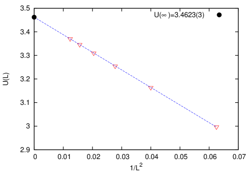
Figure 1: The fitting of Table (1) with $\mathrm{L}^{-2}$ and the extrapolated $\mathrm{U}(\infty)$ value.

3.1 The regime $\mathrm{U}\geq 0$

We start our analysis by solving numerically the Bethe ansatz equation (21) for small sizes in order to find the structure of the roots distribution for low-lying states. As expected we find that the ground state sits in the sector with zero magnetization $n=0$. In Figures (2,3) we exhibit the ground state roots in the complex plane for $\mathrm{L}=4,6$.

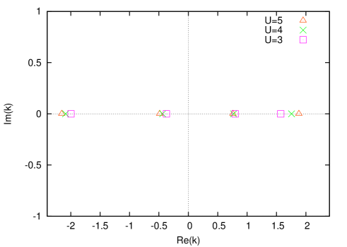
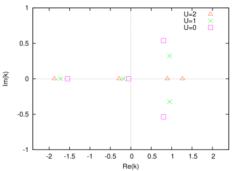
Figure 2: Ground state Bethe roots for $\mathrm{L}=4$ and for some values of $\mathrm{U}\geq 0$.

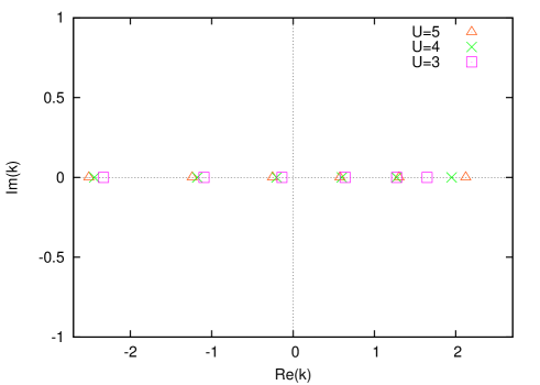
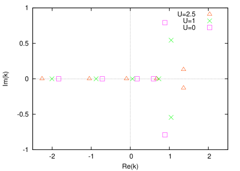
Figure 3: Ground state Bethe roots for $\mathrm{L}=6$ and for some values of $\mathrm{U}\geq 0$.

We note that the Bethe roots are real until we reach some value of $\mathrm{U}$ and after this critical point a pair of real zeros combine together to form a string of length two. As we increase the lattice size such critical point appears to grow slowly towards an irrational number which we conjecture to be exactly $\mathrm{U}_{c}=2\sqrt{3}$. In order to provide some support to this expectation consider the specific example of a state at the sector $n=\mathrm{L}-2$ built out of the complex pair $k_{1}=\alpha-\mathbf{\imath}\beta$ and $k_{2}=\alpha+\mathbf{\imath}\beta$. We can assume $\beta>0$ without any loss of generality. For large sizes the left hand side of the Bethe equation (21) for $k_{1}$ grows exponentially with $\mathrm{L}$. The only way to fulfill this behaviour is that the respective right hand side becomes exponentially close to a pole, namely

$$\sin(k_{1}-\pi/6)\exp(\mathbf{\imath}\pi/3)=\sin(k_{2}-\pi/6)/\exp(\mathbf{\imath}\pi/3)+\mathbf{\imath}\mathrm{U}/{2}+\mathcal{O}\left[\exp(-\mathrm{L})\right]$$ (24)

By the same token, for the root $k_{2}$ we expect that the right hand side goes to zero which leads us to the same condition (24). From our numerical solution we see that near to the critical point the imaginary part of the roots is very small and therefore the trigonometric functions should be limited by a unity. Taking this fact into account in Eq.(24) we obtain the following bound for the coupling,

$$\mathrm{U}\leq 2\left[\frac{\exp(\mathbf{\imath}\pi/3)-\exp(-\mathbf{\imath}\pi/3)}{\mathbf{\imath}}\right]=2\sqrt{3}$$ (25)

Another piece of evidence comes from our numerical solution of the Bethe equations for large lattice sizes. We have verified that real roots are indeed stable solutions in the range $\mathrm{U}\geq 2\sqrt{3}$ up to $\mathrm{L}=1024$ sites. Now suppose we have at hand the real roots solution at $\mathrm{U}_{c}$ for some large enough lattice size. When we try to iterate it in order to obtain the solution on the neighborhood $\mathrm{U}=2\sqrt{3}-\epsilon$ we find out that the first two largest positive roots get very close to each other even for small $\epsilon$. By increasing $\epsilon$, instead of having coincident real roots, we noticed that such pair of roots will give rise to a string with a small non-zero imaginary part. This scenario can be seen already for $\mathrm{L}=14$ as illustrated in Figures (4).

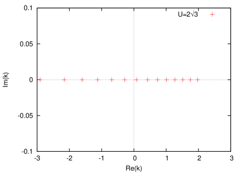
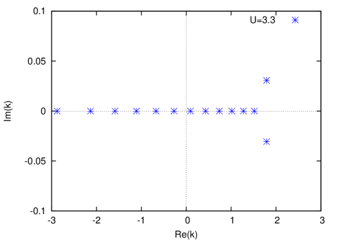
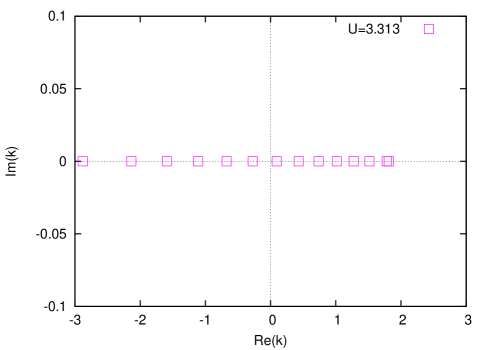
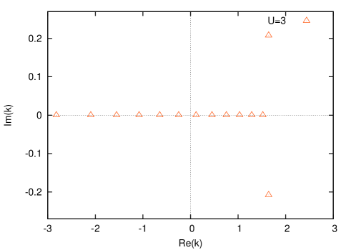
Figure 4: Ground state Bethe roots for $\mathrm{L}=14$ and for some values of $\mathrm{U}$ close to $\mathrm{U}_{c}$.

The dependence of the Bethe roots configurations on the coupling $\mathrm{U}$ tells us that the low-energy properties of the spin chain have to be studied separately in the two distinct intervals: $\mathrm{U}\geq 2\sqrt{3}$ and $0\leq\mathrm{U}<2\sqrt{3}$. We shall see below that the spin chain has a gap for first range of the coupling while appears to be massless on the second one.

3.1.1 The range $\mathrm{U}\geq 2\sqrt{3}$

In this case we have found that the scenario described above for the ground state remains valid for the lowest state in each sector $n$. These states are all described by real solutions to the Bethe equations. Therefore we can take the logarithm of Eq.(21) and as result we obtain,

$$\mathrm{L}k_{j}=2\pi Q_{j}+2\sum_{i=1}^{\mathrm{L}-n}\arctan\left[\frac{\sin(k_{j}-\pi/6)-\sin(k_{i}-\pi/6)}{\sqrt{3}\left[\sin(k_{j}-\pi/6)+\sin(k_{i}-\pi/6)\right]-\mathrm{U}}\right],~{}~{}j=1,\dots,\mathrm{L}-n,$$ (26)

where the numbers $Q_{j}$ define the different branches of the logarithm and they have to be chosen integer or half-integer according to the rule,

$$Q_{j}=\frac{\mathrm{L}-n-1}{2}-(j-1),~{}~{}j=1,\dots,\mathrm{L}-n.$$ (27)

In the thermodynamic limit the solutions $k_{j}$ become continuously distributed on some interval $k_{min}\leq k\leq k_{max}$ with a density of roots $\sigma(k)$. By taking the difference between next neighbors roots satisfying Eq.(26) one gets an integral equation for such density function which is,

$$2\pi\sigma(k)=1+2\cos(k-\pi/6)\int_{k_{min}}^{k_{max}}\frac{\left[\mathrm{U}+\sqrt{3}\mathrm{F}_{-}(k,k^{{}^{\prime}})-\sqrt{3}\mathrm{F}_{+}(k,k^{{}^{\prime}})\right]}{[\mathrm{F}_{-}(k,k^{{}^{\prime}})]^{2}+[\mathrm{U}-\sqrt{3}\mathrm{F}_{+}(k,k^{{}^{\prime}})]^{2}}\sigma(k^{{}^{\prime}})dk^{{}^{\prime}},$$ (28)

where the kernel functions are defined by,

$$\mathrm{F}_{\pm}(x,y)=\sin(x-\pi/6)\pm\sin(y-\pi/6).$$ (29)

The integrate density gives the total number of roots per site which is fixed by the range of integration. For the ground state we have the constraint,

$$\int_{k_{min}}^{k_{max}}\sigma(k)dk=1.$$ (30)

We have solved Eqs.(28) by iterative numerical integration and found out that the condition (30) is satisfied provide we set $[k_{min},k_{max}]=[k_{0},k_{0}+2\pi]$ where $k_{0}\in\mathbb{R}$ is an arbitrary integration point. In Figure (5) we have plotted the pattern of $\sigma(k)$ on a symmetrical interval with the choice $k_{0}=-\pi$.

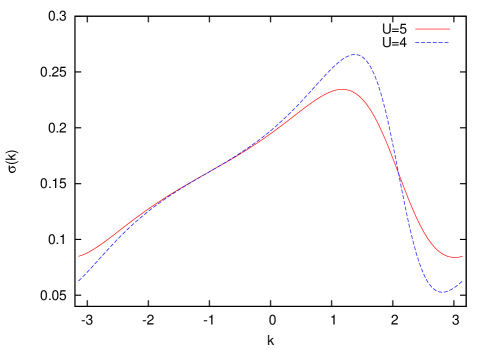
Figure 5: The root density $\sigma(k)$ for $\mathrm{U}=5$ and $\mathrm{U}=4$.

The expression for the ground state energy per site $e_{0}(\mathrm{U})$ is derived from Eq.(22). In the thermodynamic limit $\mathrm{L}\rightarrow\infty$ we obtain,

$$e_{0}(\mathrm{U})=-2\int_{k_{0}}^{k_{0}+2\pi}\cos(k+\pi/6)\sigma(k)dk$$ (31)

In order to illustrate the ground state behaviour we present in Table (2) the respective energy for finite sizes together with bulk value obtained from the numerical solution of the integral equation (28).

$\mathrm{E}_{0}(\mathrm{U})/\mathrm{L}$	$\mathrm{U}=5$	$\mathrm{U}=4.5$	$\mathrm{U}=4$	$\mathrm{U}=2\sqrt{3}$
8	-0.2044 6422 8606	-0.2300 4351 1273	-0.2636 1069 8228	-0.3118 1225 6414
12	-0.2012 6573 7835	-0.2248 9993 6711	-0.2560 4511 7699	-0.3024 9083 5111
16	-0.2008 2406 1600	-0.2238 7105 9808	-0.2538 9742 0183	-0.2992 6241 0687
24	-0.2007 3651 4467	-0.2235 5132 5431	-0.2528 0569 9816	-0.2969 6872 3330
64	-0.2007 3305 6600	-0.2235 2248 8844	-0.2525 4016 7269	-0.2953 9909 9678
128	-0.2007 3305 6598	-0.2235 2248 8276	-0.2525 3979 7503	-0.2952 0705 3381
256	-0.2007 3305 6598	-0.2235 2248 8276	-0.2525 3979 7464	-0.2951 5908 1267
516	-0.2007 3305 6598	-0.2235 2248 8276	-0.2525 3979 7464	-0.2951 4703 1065
1024	-0.2007 3305 6598	-0.2235 2248 8276	-0.2525 3979 7464	-0.2951 4409 6192
$e_{0}(\mathrm{U})$	-0.2007 3305 6598	-0.2235 2248 8276	-0.2525 3979 7464	-0.2951 4306 683

Table 2: Finite-size sequences for the ground state energy per site and the respective bulk values.

We observe that for first three parameter values the finite size corrections to the energy become irrelevant already after few hundred sites typical of an exponential convergence towards the thermodynamic limit. This is an indication that the low energy physics of the spin chain should be governed by massive excitations whose gap appears to decrease as we approach the critical point $\mathrm{U}_{c}=2\sqrt{3}$. In order to substantiate this expectation we have to compute the energy needed to remove one particle from the ground state. The removal of one root implies that the momenta $k_{j}^{{}^{\prime}}$ in the sector $n=1$ are shifted with respect to the ground state by small amounts,

$$k_{j}^{{}^{\prime}}=k_{j}+\frac{\delta(k_{j})}{\mathrm{L}}$$ (32)

where $k_{j}$ denotes the ground state momenta.

We now take the difference of Eq.(26) for the momenta $k_{j}^{{}^{\prime}}$ and $k_{j}$ and keep the leading term on $\delta(k_{j})$. Replacing the sums by integrals and making use of Eq.(28) we are led to the following integral equation,

$$2\pi\rho(k)=\int_{k_{min}}^{k_{max}}\cos(k^{{}^{\prime}}-\pi/6)\frac{\left[\mathrm{U}+\sqrt{3}\mathrm{F}_{-}(k,k^{{}^{\prime}})+\sqrt{3}\mathrm{F}_{+}(k,k^{{}^{\prime}})\right]}{[\mathrm{F}_{-}(k,k^{{}^{\prime}})]^{2}+[\mathrm{U}-\sqrt{3}\mathrm{F}_{+}(k,k^{{}^{\prime}})]^{2}}\rho(k^{{}^{\prime}})dk^{{}^{\prime}},$$ (33)

where $\rho(k)=\delta(k)\sigma(k)$.

The lowest energy gap $\Delta(\mathrm{U})$ is computed with the help of Eq.(22), namely

$$\Delta(\mathrm{U}) = \mathrm{E}_{1}(\mathrm{U})-\mathrm{E}_{0}(\mathrm{U})=\frac{\mathrm{U}}{2}-2\sum_{j=1}^{\mathrm{L}-1}\cos(k_{j}^{{}^{\prime}}+\pi/6)+2\sum_{j=1}^{\mathrm{L}}\cos(k_{j}+\pi/6)$$ (34)

$$= \frac{\mathrm{U}}{2}-2\cos(\pi/6)-2\sum_{j=1}^{\mathrm{L}-1}\left[\cos(k_{j}^{{}^{\prime}}+\pi/6)-\cos(k_{j}+\pi/6)\right]$$

$$= \frac{\mathrm{U}}{2}-\sqrt{3}+2\int_{k_{min}}^{k_{max}}\sin(k+\pi/6)\rho(k)$$

We have solved the integral equation (33) numerically for several values $\mathrm{U}>2\sqrt{3}$. We find that the density $\rho(k)$ is very small in the entire momenta interval and it seems reasonable to assume that this function should vanish. Taking into account this hypothesis the third term in Eq.(34) is zero and we conjecture that the gap is given by,

$$\Delta(\mathrm{U})=\frac{\mathrm{U}}{2}-\sqrt{3}.$$ (35)

In order to substantiate the above conclusion we have presented in Table (3) the finite-size sequences for the energy gap. We note that the numerical value around hundred sites is already very close to the exact prediction (35).

$\Delta(\mathrm{U})$	$\mathrm{U}=5$	$\mathrm{U}=4.5$	$\mathrm{U}=4$	$\mathrm{U}=2\sqrt{3}$
4	1.0363 1964 4464	0.8545 8007 1405	0.6921 7452 4898	0.5439 9429 5694
6	0.8733 4017 7602	0.6748 6896 6228	0.5023 06541 1977	0.3556 2898 7118
8	0.8136 3837 7809	0.5996 3177 1038	0.4144 2122 0768	0.2648 5127 5979
10	0.7886 6944 1708	0.5627 0418 0977	0.3652 8046 2750	0.2111 5429 3739
12	0.7775 9180 8258	0.5431 8460 2057	0.3349 8712 9854	0.1756 15006 7247
24	0.7680 7368 9898	0.5189 8852 1734	0.2776 5781 2737	0.0874 7009 7673
64	0.7679 4919 2567	0.5179 4924 6894	0.2679 8469 7157	0.0327 4775 5751
128	0.7679 4919 2431	0.5179 4919 2431	0.2679 4919 9834	0.01636 7736 1663
Conj.	0.7679 4919 2431	0.5179 4919 2431	0.2679 4919 2431	0.

Table 3: Finite-size sequences for the lowest energy gap and the conjectured value (35).

3.1.2 The range $0\leq\mathrm{U}<2\sqrt{3}$

In this situation we find that the numerical solution of the Bethe equations becomes very sensible with the initial guess for the roots. This makes it difficult to have an idea how the real roots bound together to form complex strings as we increase the lattice size. Besides the presence of real and two-string type of roots we can not rule out the formation of more involved bounds such as strings with multiple imaginary roots. As consequence of that we have not been able to figure out the formulation of the string hypothesis in the thermodynamic limit for this regime of the coupling. Here we have resorted to the results of the exact diagonalization of the Hamiltonian. In Table (4) we exhibit the finite size estimates for the mass gap associated to the first excited state. The extrapolated data shows that we have a very small gap for several values of the coupling suggesting that this phase should be governed by massless excitations.

$\Delta(\mathrm{U})$	$\mathrm{U}=3$	$\mathrm{U}=2$	$\mathrm{U}=1$	$\mathrm{U}=0$
4	0.4400 1651 0622	0.2935 3529 0332	0.2295 6105 6843	0.2067 1526 6807
5	0.3331 8629 3755	0.2147 7955 3874	0.1739 5124 9866	0.1566 0837 5958
6	0.2650 0019 6383	0.1685 2500 3057	0.1423 1283 0329	0.1309 7377 8878
7	0.2177 9262 8767	0.1386 4806 2734	0.1211 3457 3771	0.1117 7810 9994
8	0.1833 3776 7402	0.1180 8109 0063	0.1058 6440 2313	0.0978 6465 8974
9	0.1572 1529 3302	0.1031 7113 4329	0.0941 9346 0366	0.0869 9839 9570
10	0.1368 3356 0153	0.0918 9277 3383	0.0849 2246 3102	0.0783 3772 5112
11	0.1205 6941 4216	0.0830 5359 1425	0.0773 4872 5737	0.0712 4801 5197
12	0.1073 5348 9189	0.0759 1868 2286	0.0710 3084 7203	0.0653 4014 1516
Extrap.	0.0125($\pm 2$)	0.00095 ($\pm 1$)	0.00072 ($\pm 2$)	0.00057 ($\pm 1$)

Table 4: Finite-size sequences for the energy gap $\mathrm{E}_{1}(\mathrm{U})-\mathrm{E}_{0}(\mathrm{U})$ and the extrapolated value for $0\leq\mathrm{U}<2\sqrt{3}$.

3.2 The regime $\mathrm{U}\leq 0$

We start the analysis by solving the Bethe equations for small sizes. In Figure (6) we show the pattern of the roots for the ground state with $\mathrm{L=4}$. We note that there is a region of the coupling dominated two types of two-strings roots having different imaginary parts of the form $-a\pm\mathbf{\imath}b$ and $a\pm\mathbf{\imath}c$ such that $b-c\sim\mathrm{U}/2$. Once we decrease the value of $\mathrm{U}$ the complex pair with the lowest imaginary part breaks down giving rise to two real roots. It turns out that for negative $\mathrm{U}$ we find it difficult to obtain the solution of the Bethe equations even for small sizes. Again this fact has prevented us to make a proposal for the root distribution in the thermodynamic limit.

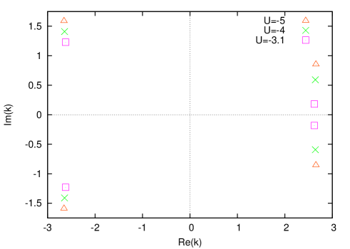
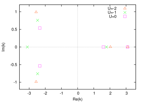
Figure 6: Ground state Bethe roots for $\mathrm{L}=4$ and for some values of $\mathrm{U}\leq 0$.

Inspite of that, the symmetry (23) suggests that conclusions for positive $\mathrm{U}$ may be achieved from the results obtained for negative $\mathrm{U}$ without the need of novel calculations. To this end we need however a correspondence connecting the low-lying eigenstates for $\mathrm{U}>0$ with the low-lying eigenstates for $\mathrm{U}<0$. Inspecting the eigenvalues of the exact diagonalization we have been able to uncover the following simple relation between the lowest energies in the sector $n=1$,

$$\mathrm{E}_{1}(\mathrm{U})-\mathrm{E}_{1}(\mathrm{-U})=\frac{\mathrm{U}}{2}\mathrm{L}$$ (36)

which was verified for even lattice sites up to $\mathrm{L}=12$ within machine precision.

This result has prompted us to look for similar connection among the ground state energies $\mathrm{E}_{0}(\mathrm{U})$ and $\mathrm{E}_{0}(-\mathrm{U})$. In Table (5) we have exhibited our numerical results for finite-size estimates $\mathrm{F}_{0}(\mathrm{U})=\mathrm{E}_{0}(\mathrm{U})-\mathrm{E}_{0}(-\mathrm{U})-\frac{\mathrm{U}}{2}\mathrm{L}$ extracted from the exact diagonalization of the Hamiltonian. Although $\mathrm{F}_{0}(\mathrm{U})$ is not exactly zero the deviation is very small indicating that Eq.(36) should be valid for the ground state in the thermodynamic limit.

$\mathrm{F}_{0}(\mathrm{U})$	$\mathrm{U}=4$	$\mathrm{U}=2\sqrt{3}$	$\mathrm{U}=\sqrt{2}$	$\mathrm{U}=1$
4	-0.0025 0261 7524	-0.0048 2183 0368	-0.0069 4028 6179	-0.0053 6392 2112
6	-0.0002 9857 8032	-0.0026 3677 4463	-0.0045 2586 3690	-0.0033 6949 6877
8	0.0004 7434 8326	-0.0015 7527 8327	-0.0029 2025 0485	-0.0021 2556 6789
10	0.0007 2533 0998	-0.0010 3343 6575	-0.0019 9639 6571	-0.0014 3687 8350
12	0.0007 8126 9945	-0.0007 2631 8473	-0.0014 4003 0532	-0.0010 3046 6004

Table 5: The finite-size sequences $\mathrm{F}_{0}(\mathrm{U})=\mathrm{E}_{0}(\mathrm{U})-\mathrm{E}_{0}(-\mathrm{U})-\frac{\mathrm{U}}{2}\mathrm{L}$.

In any case these results tells us the lowest energy gap for both $\mathrm{U}<0$ and $\mathrm{U}>0$ is certain of the same magnitude up to $\mathrm{L}=12$ sites. Assuming that this feature remains for larger sizes and considering our findings for $\mathrm{U}>0$ we expect that the low-energy behaviour of the excitations of the spin chain should be gapped for $|\mathrm{U}|>2\sqrt{3}$ while being massless in the regime $-2\sqrt{3}\leq\mathrm{U}\leq 2\sqrt{3}$.

4 Conclusions

In this work we have studied the properties of the spectrum of a three-state vertex model based on a $\mathrm{R}$-matrix which is non-additive with respect to the spectral variables. Although the vertex weights lie on a curve with genus five a substantial part of the structure of the transfer matrix eigenvalues was expressed by meromorphic functions on an elliptic curve. This is because the eigenvalues depend on very specific ratios of the weights representing a small subset of the field of fractions of the genus five curve. We have noted that change on the geometry of the weights has direct connection with the possibility of the presence of different types of physical behaviour. This feature has been investigated in the case of an underlying spin one chain by means of analytical and numerical methods. We find that the low-energy excitations can change from gapped to massless and the critical point separating such phases is exactly the same found by geometrical considerations.

There are some open problems in the analysis of spin one chain which are worth to pursue. The basis for an analytical study of the thermodynamic limit properties in the massless regime is still lacking. This is important for the derivation of the finite-size behaviour and as consequence the underlying scaling dimensions. The observed correspondence between low-lying states for positive and negative coupling deserves further investigation. It is also of interest to establish functional relations for the transfer matrix eigenvalues in the infinite system such as the so-called inversion identities [12]. This method bypass the Bethe ansatz analysis providing us an alternative way to derive the free-energy and the dispersion relation of of the low-lying excitations [13]. We hope that the results obtained here will prompt further developments and interest in the study of spin chains originated out of non-additive $\mathrm{R}$-matrices.

Appendix A: Algebraic Bethe Ansatz

In what follows we summarized the structure of the eigenvectors of the transfer matrix (2,5,1) within the general algebraic Bethe ansatz formulation devised in the work [9]. In this framework the eigenstates are expressed in terms of the elements of the monodromy matrix denoted here by ${\cal T}(\lambda)$. In the case of three state models it can generically be written as,

$${\cal T}(\lambda)=\left(\begin{array}[]{cccc}{\cal T}_{11}(\lambda)&{\cal T}_{12}(\lambda)&{\cal T}_{13}(\lambda)\\ {\cal T}_{21}(\lambda)&{\cal T}_{22}(\lambda)&{\cal T}_{23}(\lambda)\\ {\cal T}_{31}(\lambda)&{\cal T}_{32}(\lambda)&{\cal{T}}_{33}(\lambda)\\ \end{array}\right),$$ (A.1)

whose trace provides a representation for the transfer matrix,

$$\mathrm{T}(\lambda)={\cal T}_{11}(\lambda)+{\cal T}_{22}(\lambda)+{\cal T}_{33}(\lambda).$$ (A.2)

A basic condition to diagonalize the transfer matrix by the algebraic Bethe ansatz is the existence of a reference state $\left|0\right\rangle$ such that ${\cal T}(\lambda)\left|0\right\rangle$ gives a triangular matrix. In our case this pseudo vacuum can be taken as the tensor product of local ferromagnetic state,

$$\left|0\right\rangle=\prod_{i=1}^{\mathrm{L}}\otimes\left(\begin{array}[]{c}1\\ 0\\ 0\end{array}\right)_{i}.$$ (A.3)

Inspecting the action of the monodromy matrix on the pseudo vacuum $\left|0\right\rangle$ it is not difficult to derive the following identities,

$${\cal T}_{11}(\lambda)\left|0\right\rangle=\left[a(\lambda,\mu)\right]^{\mathrm{L}},~{}~{}{\cal T}_{22}(\lambda)\left|0\right\rangle=\left[{\bar{b}}(\lambda,\mu)\right]^{\mathrm{L}},~{}~{}{\cal T}_{33}(\lambda)\left|0\right\rangle=\left[f(\lambda,\mu)\right]^{\mathrm{L}},~{}~{}{\cal T}_{ij}(\lambda)\left|0\right\rangle=0~{}~{}\mathrm{for}~{}~{}i>j.$$ (A.4)

The eigenstates of $T(\lambda)$ in the sectors with total magnetization $n=\mathrm{L}-m$ are constructed in terms of a linear combination of product of creation operators defined by the first row of the monodromy matrix. These states are viewed as $m$-particle states parameterized by the number of rapidities $\lambda_{1},\dots,\lambda_{m}$ and they can be written as,

$$\left|\Phi_{m}\right\rangle=\phi_{m}(\lambda_{1},\dots,\lambda_{m})\left|0\right\rangle.$$ (A.5)

It turns out that the mathematical structure of the vector $\phi_{m}(\lambda_{1},\dots,\lambda_{m})$ is given by means of a two-step recurrence relation, namely

$$\phi_{m}(\lambda_{1},\dots,\lambda_{m}) = {\cal T}_{12}(\lambda_{1})\phi_{m-1}(\lambda_{2},\dots,\lambda_{m})-{\cal T}_{13}(\lambda_{1})\sum_{j=2}^{m}\varepsilon\frac{d(\lambda_{1},\lambda_{j})}{f(\lambda_{1},\lambda_{j})}\phi_{m-2}(\lambda_{2},\dots,\lambda_{j-1},\lambda_{j+1},\dots,\lambda_{m})$$ (A.6)

$$\times {\cal T}_{1,1}(\lambda_{j})\prod_{\stackrel{{\scriptstyle k=2}}{{k\neq j}}}^{m}\frac{a(\lambda_{k},\lambda_{j})}{\bar{b}(\lambda_{k},\lambda_{j})}\theta_{<}(\lambda_{k},\lambda_{j}),$$

which is a non-trivial generalization of a previous work by Tarasov [14].

The permutation function $\theta_{<}(\lambda_{i},\lambda_{j})$ entering Eq.(A.6) is defined as,

$$\theta_{<}(\lambda_{i},\lambda_{j})=\begin{cases}\displaystyle\theta(\lambda_{i},\lambda_{j}),~{}~{}~{}~{}\mbox{for}~{}~{}i<j\cr\displaystyle 1,~{}~{}~{}~{}\mbox{for}~{}~{}i\geq j.\end{cases}$$ (A.7)

where the expression for $\theta(\lambda_{i},\lambda_{j})$ in terms of the weights has been given in Eq.(8).

We observe that the above vector can be related to each other under permutation of the rapidities,

$$\phi_{m}(\lambda_{1},\dots,\lambda_{j},\lambda_{j+1},\dots,\lambda_{m})=\theta(\lambda_{j},\lambda_{j+1})\phi_{m}(\lambda_{1},\dots,\lambda_{j+1},\lambda_{j},\dots,\lambda_{m})$$ (A.8)

The condition that the off-shell multiparticle states (A.5,A.6) are in fact eigenstates of the transfer matrix imposes restrictions on the rapidities $\lambda_{1},\dots,\lambda_{m}$. These are the Bethe equations already presented in the main text, see Eq.(9).

References

- [1] R.J. Baxter, Exactly Solved Models in Statistical Mechanics, Academic Press, New York, 1982
- [2] E.K. Sklyanin, L.A. Takhtadzhyan and L.D. Faddeev, Theor.Math.Fiz. 40 (1979) 194
- [3] M. Lüscher, Nucl.Phys.B 117 (1976) 475
- [4] V.O. Tarasov, L.A. Takhtadzhyan and L.D. Faddeev, Theor.Math.Fiz. 57 (1983) 163
- [5] B.S. Shastry, J.Stat.Phys. 30 (1988) 57
- [6] M.J. Martins and P.B. Ramos, Nucl.Phys.B (1998) 413
- [7] M.J. Martins, Nucl.Phys.B 874 (2013) 243
- [8] V.E. Korepin, G. Izergin and N.M. Bogoliubov Quantum Inverse Scattering Method, Correlation Functions and Algebraic Bethe ansatz, Cambridge University Press, Cambridge, 1992.
- [9] C.S. Melo and M.J. Martins, Nucl.Phys.B 806 (2009) 567
- [10] W. Fulton, Algebraic Curves , W.A. Benjamin, New York, 1969.
- [11] C. Crampé, L. Frappat and E. Ragoucy, J.Phys.A 46 (2013) 405001, W.A. Benjamin, New York, 1969.
- [12] Y.G. Strogonov, Phys.Lett.A 74 (1979) 116, R.J. Baxter, J.Stat.Phys. 28 (1982) 1
- [13] A. Kumpler, J.Phys.A:Math.Gen. 23 (1990) 809
- [14] V.O. Tarasov, Ther.Math.Phys. 76 (1988) 793