Forecasted masses for seven thousand KOIs

Abstract

Recent transit surveys have discovered thousands of planetary candidates with directly measured radii, but only a small fraction have measured masses. Planetary mass is crucial in assessing the feasibility of numerous observational signatures, such as radial velocities (RVs), atmospheres, moons and rings. In the absence of a direct measurement, a data-driven, probabilistic forecast enables observational planning and so here we compute posterior distributions for the forecasted mass of approximately seven thousand Kepler Objects of Interest (KOIs). Our forecasts reveal that the predicted RV amplitudes of Neptunian planets are relatively consistent, as a result of transit survey detection bias, hovering around the few m/s level. We find that mass forecasts are unlikely to improve through more precise planetary radii, with the error budget presently dominated by the intrinsic model uncertainty. Our forecasts identify a couple of dozen KOIs near the Terran-Neptunian divide with particularly large RV semi-amplitudes which could be promising targets to follow-up, particularly in the near-IR. With several more transit surveys planned in the near-future, the need to quickly forecast observational signatures is likely to grow and the work here provides a template example of such calculations.

1 Introduction

Two of the most fundamental properties of any planet are its mass and radius. Unfortunately, for the vast majority of the thousands of planetary candidates discovered by Kepler (Coughlin et al., 2016), we only have measurements of planetary radii. Whilst a direct measurement of mass is always preferable, predicting a planet’s mass based off its radius is often useful. Specifically, there are numerous follow-up observations for which the predicted signal-to-noise depends strongly upon the planetary mass.

This is particularly important because Kepler has delivered so many planetary candidates that it is often impractical to schedule follow-up of every object. Finite resources demand prioritization and one obvious criteria for ranking the objects is whether an observational signature is even expected to be detectable.

We highlight several effects where planetary mass directly controls the amplitude and/or feasibility, such as radial velocity semi-amplitude (Struve, 1952), astrometric amplitude (Jacob, 1855), transit spectroscopy scale heights (Seager & Sasselov, 2000), Doppler beaming (Rybicki & Lightman, 1979), ellipsoidal variations (Kopal, 1959), transit timing variations (Holman & Murray, 2005; Agol et al., 2005), stability of rings (Schlichting & Chang, 2011), stability of exomoons (Barnes & O’Brien, 2002) and detectability of exomoons (Kipping, 2009a, b).

In each case, it is generally preferable to estimate a credible interval for the planetary mass, rather than a point estimate. Such a credible interval describes the probable range (at some chosen level of confidence), ideally accounting for both the present measurement error on the planetary radius and also the inherent uncertainty caused by using what, practically speaking, will always be an imperfect predictive model. In statistical parlance, what we are really describing here is generating posterior samples for the predicted mass using a probabilistic model conditioned upon posterior samples of the observed planetary radius. In this way, we explicitly acknowledge that our predictions are conditioned not just upon a measured radius with finite uncertainty, but also upon a model which too has finite uncertainty.

Probabilistic forecasts made in this way allow for more robust and accurate predictions, albeit at the expense of larger credible intervals, as first highlighted by Wolfgang & Rogers & Ford (2016). Whilst it has become increasingly common practice for the exoplanet community to share posterior distributions of measured parameters such as planetary radii (e.g. Rowe & Thompson 2015; Foreman-Mackey et al. 2016; Kipping et al. 2017), there remains a paucity of probabilistic models able to convert these measurements into a planetary mass, with most mass-radius relations still relying on deterministic formalisms (e.g. recent examples Weiss & Marcy 2014; Hatzes & Rauer 2015; Millis & Mazeh 2017).

The recent availability of a homogeneous set of joint posteriors for Kepler host stars (Mathur et al., 2017) and associated transit parameters (Rowe & Thompson, 2015), combined with the first probabilistic forecasting mass-radius relation spanning the entire planetary regime (Chen & Kipping, 2017), finally enables mass forecasts for thousands of planetary candidates. In this work, we forecast the mass of approximately seven thousand Kepler Objects of Interest (KOIs), described in detail in Section 2. We highlight some important implications and patterns evident from our analysis in Section 3, before framing our results in a broader context in Section 4.

2 Forecasting KOI Masses

2.1 Data Requirements

The principal objective of this work is to compute self-consistent and homogeneous a-posteriori distributions for the predicted mass of each KOI. The predicted mass of each KOI will be solely determined by its radius and the empirical, probabilistic forecasting model of Chen & Kipping (2017). Because of this conditional relationship, then mass and radius will certainly be covariant, along with any other derived terms based on these quantities. We therefore aim to derive the joint posteriors for all the parameters of interest, which will encode any resulting covariances.

To accomplish this goal, we first require posterior distributions for the KOI radii. The transit light curve of each KOI enables a measurement of the planet-to-star radius ratio, $p$, with the precision depending upon photometric quality, number and duration of observed transit events and modest degeneracies with other covariant terms describing the transit shape (Carter et al., 2008). With the quantity $p$ in-hand, it may be combined with the stellar radius, $R_{\star}$, to infer the true planetary size, $R_{P}$. Therefore, to make progress we need homogenous posterior probability distributions for 1) basic transit parameters of each KOI 2) fundamental stellar properties of each KOI.

2.2 Transit Posteriors

Basic transit parameters of each KOI are provided in the NASA Exoplanet Archive (NEA, Akeson et al. 2013), but these are summary statistics rather than full posterior distributions, as required for this work. Fortunately, Rowe & Thompson (2015) provide posterior distributions for almost every KOI, with 100,000 samples for each obtained via a Markov Chain Monte Carlo (MCMC) regression of a Mandel & Agol (2002) light curve model to the Kepler photometric times series (we direct the reader to Rowe & Thompson 2015 for details). We downloaded all available posteriors and found 7106 object files.

Except for two KOIs, all of these objects appear in the currently listed NEA database (comprising of 9564 KOIs), with the exceptions being KOI-1168.02 and KOI-1611.02. We deleted these two objects from our sample in what follows, giving us 7104 KOIs. The other 2460 KOIs were not modeled by Rowe & Thompson (2015) and thus are not considered further in what follows.

2.3 Stellar Posteriors

For stellar properties, we again note that summary statistics are available on NEA but posteriors are not directly available. As one of our criteria is a homogenous set of of posteriors, and we wish to calculate masses for as many KOIs as possible, inferences for particular subsets of the KOI database are not as useful for this work. Instead, we used the publicly available posteriors from Mathur et al. (2017) who use information such as colors, spectroscopy and asteroseismology to fit Dartmouth isochrone models (Dotter et al., 2008) for each Kepler star, giving 40,000 posterior samples per star.

We attempted to download stellar posteriors for all 7104 KOIs in the Rowe & Thompson (2015) database, but found that posteriors were missing for 93 KOIs spanning 87 stars. These KOIs are flagged with a “1” in Table 1 and were not considered further for analysis.

Table 1: Data flags assigned to 7104 KOIs considered in this analysis. “0” denotes no problems, “1” denotes that stellar posteriors were missing and “2” denotes transit posteriors were missing. Only a portion of the table is shown here, the full version is available in the online version.

KOI	data flag
0001.01	0
0002.01	0
0003.01	0
0004.01	0
0005.01	0
0005.02	2
0006.01	0
0007.01	0
0008.01	0
0009.01	0
0010.01	0
⋮	⋮

2.4 KOI Radii Posteriors

We next combined these distributions together to generate fair realizations of the KOI radii. We do this by consecutively stepping through each row of the Mathur et al. (2017) samples and drawing a random row from the corresponding Rowe & Thompson (2015) posterior samples for $p$. This is possible because the two posteriors are completely independently and share no covariances.

This process results in 40,000 fair realizations for the radius of each KOI, where we report the radii in units of Earth radii ($R_{\oplus}=6378.1$ km), which are made available in the public posteriors available at this URL(https://github.com/chenjj2/forecasts).

During this process, we found 38 KOIs could not locate the corresponding MCMC file for the Rowe & Thompson (2015) transit parameters. It is unclear why these were missing but given their relativity small number, we simply flag them with a “2” in Table 1 and do not consider them further for analysis. At this point, we are left with 6973 KOIs for which we have been able to derive a radius posterior, of which 2283 are dispositioned as “CONFIRMED” on NEA, 1665 are “CANDIDATE” and 3025 are “FALSE POSITIVE” (these dispositions are also provided in Table 2).

2.5 Predicting Masses with forecaster

The next step is to take the radius posterior of each KOI and, row-by-row, predict a corresponding predicted mass with forecaster. Whilst we direct the reader to Chen & Kipping (2017) for a full description of forecaster, we here briefly describe the model and how it was calibrated. We also direct the reader to Wolfgang & Rogers & Ford (2016) for their prior and alternative discussion of probabilistic mass-radius relations.

forecaster is fundamentally probabilistic, by which we mean that the model includes intrinsic dispersion in the mass-radius relation to account for additional variance beyond measurement uncertainties. This dispersion represents the variance observed in nature itself. In contrast, a deterministic model, in the case of a simple power-law, would be given by

$$\frac{R}{R_{\oplus}}=C\Big{(}\frac{M}{M_{\oplus}}\Big{)}^{S},$$ (1)

where $R$ & $M$ are the mass and radius of the object and $C$ & $S$ are the parameters of the power-law. In this relation, a single radius value corresponds to a single mass, once the shape parameters have been trained. However, in reality of course, two planets could have the same masses but different radii due to, for example, distinct compositions. The power of the probabilistic formalism is to catch the intrinsic variance between different planets, essentially adding an extra noise term which absorbs our ignorance of the true model. Following Chen & Kipping (2017), we substitute $\mathcal{M}$ and $\mathcal{R}$ represent $\log_{10}(M/M_{\oplus})$ and $\log_{10}(R/R_{\oplus})$ respectively, to write our probabilistic model as

$$\mathcal{R}\sim\mathcal{N}(\mu=\mathcal{C}+\mathcal{M}\times S,\sigma=\sigma_{\mathcal{R}})$$ (2)

where $\mathcal{C}=\log_{10}C$ and $\mathcal{N}(\mu,\sigma)$ is a normal distribution. The model is also empirical because it is derived by fitting the above mass-radius relation conditioned on a sample of 316 well-constrained objects, with detailed tests in Chen & Kipping (2017) demonstrating that the sample provides an unbiased training set.

Another characteristic of forecaster is that it was only trained within a specific (albeit broad) mass range, from $3\times 10^{-4}\ M_{\oplus}$ to $3\times 10^{5}\ M_{\oplus}$, corresponding to dwarf planets to late-type stars. However, some extreme KOIs have radii which fall outside of the expected corresponding radius range. To enable a homogeneous analysis, we simply extend the first and last part of the broken power-law relation, so that it could cover a semi-infinite interval. In practice, this is only necessary for very large KOIs exceeding a Solar radius, for which the KOI cannot be a planet in any case, and thus these extrapolations simply highlight the unphysical nature of these rare cases.

As discussed earlier, the model was applied to each radius posterior sample for each KOI (278.92 million individual forecasts). It is important to stress that the probabilistic nature of forecaster means that re-running the same script again on the same KOI would lead to a slightly different set of posterior samples for the planetary mass, although they would still of course be fair and representative samples.

The 68.3% credible intervals of the forecasted masses are depicted in upper panel of Figure 1 and listed along with the 95.5% credible intervals in Table 2.

To perform the analysis, we used the function "Rpost2M" in forecaster. To be clearer, a summary of the steps taken in the function is listed as below. 1. generates a grid of mass in the allowed mass range 2. calculates the probabilities of the measured radius given each mass in the grid 3. use the above probabilities as weights to redraw mass For more details, we direct the reader to the original forecasterpaper Chen & Kipping (2017).

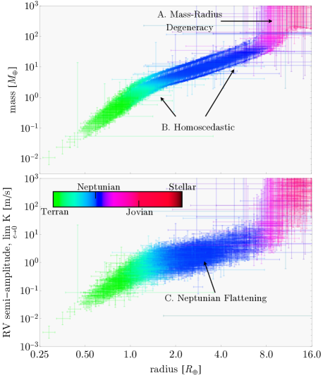
Figure 1: Forecasted masses (top) and radial velocity semi-amplitudes (bottom) for a circular orbit, as a function of the observed KOI radius. We here only show objects with a NEA disposition of being either a candidate or validated planet. Error bars depict the 68.3% credible intervals.

Table 2: Final predicted properties for 6973 KOIs using forecaster. Quoted values are the [$-2,-1,0,+1,+2$] $\sigma$ credible intervals. First letter of the flag column gives modal planet classification (“T”=Terran, “N”=Neptunian, “J”=Jovian & “S”=Stellar). Second letter of the flag column denotes NEA KOI disposition where “f” is a false-positive, “c” is a candidate and “v” is validated/confirmed. Only a portion of the table is shown here, the full version is available in the online version.

KOI	flag	$\log_{10}(R_{P}$ $[R_{\oplus}])$	$\log_{10}(M_{P}$ $[M_{\oplus}])$	$\log_{10}(K\,[\mathrm{m}\,\mathrm{s}^{-1}])$	$\log_{10}(\rho_{P}\,[\mathrm{g}\,\mathrm{cm}^{-3}])$	$\log_{10}(g_{P}\,[\mathrm{cm}\,\mathrm{s}^{-2}])$
0001.01	Jv	[1.08,1.10,1.11,1.13,1.15]	[1.83,2.33,3.20,4.14,4.53]	[1.51,2.02,2.88,3.82,4.19]	[-0.77,-0.27,0.60,1.55,1.93]	[2.59,3.09,3.96,4.91,5.29]
0002.01	Jv	[1.16,1.18,1.20,1.22,1.24]	[1.86,2.23,2.95,4.51,4.67]	[1.44,1.82,2.54,4.08,4.22]	[-1.01,-0.63,0.09,1.63,1.79]	[2.44,2.82,3.54,5.09,5.24]
0003.01	Nv	[0.66,0.67,0.69,0.70,0.71]	[0.81,1.07,1.32,1.58,1.83]	[0.45,0.71,0.96,1.21,1.46]	[-0.49,-0.23,0.01,0.26,0.51]	[2.43,2.69,2.94,3.19,3.44]
0004.01	Jc	[0.85,0.92,1.00,1.08,1.17]	[1.34,1.72,3.04,4.13,4.46]	[0.90,1.27,2.55,3.64,3.95]	[-0.76,-0.39,0.64,1.83,2.22]	[2.47,2.82,3.94,5.10,5.43]
0005.01	Nc	[0.83,0.85,0.87,0.89,0.91]	[1.13,1.40,1.67,2.00,4.28]	[0.64,0.91,1.18,1.51,3.77]	[-0.73,-0.46,-0.19,0.14,2.37]	[2.38,2.65,2.92,3.25,5.51]
0006.01	Sf	[1.21,1.38,1.60,1.91,2.10]	[2.10,4.77,5.05,5.39,5.48]	[1.83,4.46,4.69,4.96,5.03]	[-1.05,0.23,0.89,1.30,1.56]	[2.48,4.43,4.79,4.99,5.12]
0007.01	Nv	[0.58,0.60,0.62,0.65,0.67]	[0.70,0.96,1.22,1.47,1.73]	[0.31,0.57,0.82,1.07,1.32]	[-0.42,-0.16,0.08,0.34,0.59]	[2.45,2.71,2.96,3.21,3.46]
0008.01	Nf	[0.19,0.22,0.26,0.32,0.38]	[0.26,0.44,0.66,0.90,1.17]	[0.06,0.24,0.45,0.70,0.97]	[0.15,0.37,0.60,0.84,1.09]	[2.71,2.90,3.11,3.35,3.60]
0009.01	Jf	[0.99,1.06,1.15,1.27,1.37]	[1.77,2.26,3.27,4.56,4.80]	[1.32,1.80,2.83,4.08,4.24]	[-1.07,-0.48,0.62,1.62,1.97]	[2.41,2.92,4.00,5.10,5.30]
0010.01	Jv	[1.11,1.14,1.17,1.20,1.23]	[1.85,2.27,3.03,4.23,4.63]	[1.43,1.85,2.61,3.81,4.17]	[-0.93,-0.50,0.27,1.50,1.85]	[2.49,2.92,3.69,4.91,5.26]
0011.01	Sf	[0.77,0.93,1.18,1.51,1.76]	[1.32,1.86,3.78,4.95,5.24]	[0.97,1.51,3.43,4.52,4.75]	[-1.04,-0.35,0.85,1.53,2.08]	[2.41,2.87,4.62,5.05,5.33]
0012.01	Jv	[1.09,1.13,1.17,1.21,1.27]	[1.86,2.27,3.04,4.31,4.67]	[1.14,1.56,2.34,3.59,3.91]	[-0.96,-0.51,0.29,1.55,1.85]	[2.47,2.91,3.70,4.99,5.26]
0013.01	Jv	[1.05,1.12,1.21,1.32,1.50]	[1.87,2.29,3.35,4.71,4.95]	[1.42,1.85,2.93,4.21,4.36]	[-1.13,-0.55,0.61,1.57,1.85]	[2.38,2.88,4.02,5.10,5.25]
0014.01	Nf	[0.55,0.62,0.69,0.80,0.90]	[0.77,1.05,1.35,1.65,2.04]	[0.29,0.57,0.85,1.14,1.52]	[-0.57,-0.28,-0.00,0.27,0.65]	[2.42,2.69,2.94,3.20,3.56]
0015.01	Sf	[1.45,1.70,2.02,2.28,2.46]	[2.01,4.96,5.40,5.48,5.48]	[1.42,4.40,4.75,4.83,4.86]	[-4.55,-0.66,0.12,0.79,1.25]	[0.14,3.87,4.39,4.75,4.97]
0016.01	Sf	[0.79,1.01,1.64,1.94,2.13]	[1.36,2.49,5.09,5.42,5.48]	[1.06,2.15,4.70,4.97,5.02]	[-0.76,-0.09,0.59,1.22,1.87]	[2.53,3.29,4.63,4.92,5.19]
0017.01	Jv	[1.08,1.10,1.13,1.15,1.19]	[1.82,2.32,3.14,4.14,4.56]	[1.44,1.93,2.76,3.75,4.14]	[-0.82,-0.33,0.51,1.52,1.91]	[2.56,3.04,3.88,4.89,5.28]
0018.01	Jv	[1.12,1.14,1.18,1.21,1.24]	[1.86,2.27,3.01,4.29,4.64]	[1.41,1.81,2.56,3.83,4.15]	[-0.95,-0.52,0.23,1.53,1.84]	[2.49,2.90,3.65,4.95,5.25]
0019.01	Sf	[0.96,1.12,1.32,1.45,1.56]	[1.77,2.39,4.67,4.88,5.03]	[1.55,2.16,4.40,4.59,4.70]	[-1.30,-0.40,1.23,1.52,1.88]	[2.28,3.00,4.92,5.08,5.23]
0020.01	Jv	[1.11,1.16,1.23,1.30,1.38]	[1.86,2.25,3.25,4.68,4.82]	[1.43,1.82,2.82,4.20,4.31]	[-1.18,-0.65,0.42,1.59,1.79]	[2.35,2.81,3.86,5.11,5.23]
0021.01	Sf	[1.22,1.35,1.51,1.69,1.87]	[2.04,4.73,4.95,5.16,5.37]	[1.64,4.28,4.46,4.63,4.78]	[-1.22,0.63,1.07,1.37,1.58]	[2.35,4.66,4.88,5.02,5.14]
0022.01	Jv	[1.01,1.05,1.09,1.16,1.23]	[1.74,2.29,3.24,4.20,4.57]	[1.22,1.76,2.71,3.65,4.00]	[-0.84,-0.31,0.70,1.67,2.00]	[2.53,3.05,4.04,5.02,5.32]
0023.01	Jf	[1.14,1.19,1.24,1.30,1.38]	[1.86,2.23,3.24,4.69,4.82]	[1.37,1.74,2.76,4.16,4.26]	[-1.19,-0.71,0.35,1.60,1.77]	[2.34,2.76,3.81,5.12,5.22]
0024.01	Jf	[0.83,0.89,0.98,1.09,1.20]	[1.28,1.64,2.74,4.10,4.47]	[1.03,1.38,2.46,3.82,4.17]	[-0.78,-0.42,0.29,1.80,2.24]	[2.44,2.77,3.60,5.08,5.44]
0025.01	Sf	[1.22,1.29,1.37,1.49,1.62]	[1.93,2.74,4.78,4.93,5.09]	[1.55,2.38,4.35,4.46,4.57]	[-1.37,-0.32,1.29,1.50,1.64]	[2.23,3.19,4.97,5.09,5.17]
0026.01	Jf	[0.94,1.00,1.09,1.23,1.41]	[1.61,2.18,3.33,4.41,4.84]	[1.01,1.53,2.70,3.77,4.12]	[-0.97,-0.39,0.81,1.68,2.08]	[2.45,2.95,4.15,5.09,5.35]
0027.01	Sf	[1.83,1.89,1.97,2.09,2.23]	[5.27,5.36,5.44,5.48,5.48]	[4.95,5.01,5.05,5.08,5.10]	[-0.46,-0.04,0.27,0.45,0.58]	[4.01,4.28,4.48,4.59,4.67]
0028.01	Sf	[1.68,1.73,1.82,1.94,2.06]	[5.10,5.19,5.30,5.43,5.48]	[4.62,4.68,4.76,4.83,4.87]	[0.01,0.33,0.58,0.74,0.87]	[4.32,4.52,4.64,4.74,4.81]
0031.01	Sf	[1.59,1.65,1.72,1.80,1.88]	[5.00,5.09,5.19,5.30,5.39]	[4.72,4.79,4.85,4.92,4.98]	[0.45,0.60,0.76,0.91,1.04]	[4.56,4.65,4.73,4.81,4.89]
0033.01	Sf	[1.58,1.62,1.68,1.74,1.78]	[4.98,5.05,5.13,5.22,5.30]	[4.84,4.89,4.94,4.98,5.03]	[0.62,0.72,0.84,0.96,1.06]	[4.63,4.70,4.77,4.84,4.91]
0041.01	Nv	[0.30,0.32,0.35,0.37,0.40]	[0.33,0.53,0.77,1.01,1.26]	[-0.24,-0.04,0.18,0.42,0.67]	[0.02,0.24,0.47,0.71,0.96]	[2.63,2.84,3.06,3.30,3.55]
0041.02	Nv	[0.06,0.09,0.11,0.15,0.19]	[-0.00,0.17,0.35,0.59,0.86]	[-0.49,-0.31,-0.14,0.10,0.36]	[0.41,0.58,0.74,0.97,1.23]	[2.78,2.95,3.10,3.34,3.60]
0041.03	Nv	[0.12,0.14,0.17,0.20,0.25]	[0.14,0.31,0.49,0.73,0.98]	[-0.59,-0.42,-0.24,-0.00,0.25]	[0.36,0.54,0.72,0.94,1.20]	[2.80,2.96,3.14,3.36,3.62]
0042.01	Nv	[0.35,0.37,0.39,0.41,0.43]	[0.37,0.59,0.83,1.07,1.33]	[-0.28,-0.06,0.16,0.41,0.67]	[-0.04,0.17,0.41,0.65,0.91]	[2.59,2.81,3.04,3.29,3.55]
0044.01	Jf	[0.98,1.03,1.10,1.19,1.31]	[1.71,2.26,3.27,4.29,4.71]	[0.91,1.43,2.45,3.47,3.81]	[-0.92,-0.37,0.70,1.67,2.03]	[2.48,2.99,4.06,5.08,5.33]
0046.01	Nv	[0.58,0.64,0.70,0.78,0.85]	[0.80,1.08,1.36,1.64,1.93]	[0.42,0.70,0.97,1.24,1.52]	[-0.55,-0.28,-0.01,0.24,0.53]	[2.43,2.68,2.94,3.19,3.45]
0046.02	Tv	[-0.11,-0.05,0.01,0.09,0.17]	[-0.52,-0.24,0.06,0.40,0.73]	[-0.98,-0.70,-0.40,-0.08,0.23]	[0.40,0.57,0.73,0.94,1.31]	[2.62,2.81,3.01,3.24,3.58]
0048.01	Nf	[2.07,2.27,2.53,2.86,3.11]	[1.91,2.04,2.13,5.48,5.48]	[1.25,1.38,1.48,4.64,4.67]	[-6.48,-5.73,-4.74,-0.59,-0.01]	[-1.12,-0.62,0.03,3.92,4.31]
0049.01	Nv	[0.41,0.43,0.47,0.51,0.55]	[0.47,0.71,0.95,1.22,1.48]	[-0.03,0.19,0.44,0.70,0.96]	[-0.19,0.04,0.29,0.54,0.80]	[2.53,2.76,3.01,3.26,3.51]
0052.01	Jf	[1.18,1.22,1.26,1.31,1.41]	[1.86,2.22,3.40,4.71,4.86]	[1.56,1.91,3.10,4.35,4.46]	[-1.22,-0.79,0.44,1.60,1.73]	[2.31,2.71,3.93,5.13,5.21]
0061.01	Sf	[1.11,1.41,1.75,2.01,2.18]	[2.14,4.81,5.21,5.46,5.48]	[1.85,4.49,4.82,4.99,5.03]	[-0.86,0.04,0.61,1.19,1.56]	[2.64,4.31,4.65,4.93,5.11]
0063.01	Nv	[0.71,0.73,0.77,0.81,0.85]	[0.95,1.21,1.46,1.72,1.99]	[0.45,0.71,0.97,1.22,1.49]	[-0.61,-0.35,-0.09,0.15,0.42]	[2.41,2.67,2.92,3.17,3.43]
0064.01	Nc	[0.81,0.86,0.91,0.96,1.03]	[1.18,1.48,1.82,3.89,4.37]	[0.86,1.15,1.48,3.54,4.00]	[-0.74,-0.45,-0.11,1.79,2.32]	[2.40,2.69,3.02,4.99,5.49]
0066.01	Sf	[2.11,2.19,2.28,2.35,2.42]	[1.94,2.10,5.47,5.48,5.48]	[1.69,1.85,5.11,5.13,5.14]	[-4.43,-4.15,-0.63,-0.36,-0.11]	[0.21,0.42,3.90,4.07,4.24]
⋮	⋮	⋮	⋮	⋮	⋮	⋮

3 Implications & Limitations

3.1 Densities, Gravities and RV Amplitudes

With a joint posterior for the both the stellar and planetary fundamental parameters in hand, we can compute other derived quantities of interest, such as surface gravity, bulk density and radial velocity (RV) amplitude (these are given in Table 2). Once again, we stress that these values should be treated as forecasts and not measurements.

We have computed forecasted masses for all KOIs where available, irrespective of whether the KOI is a known false-positive or confirmed planet. False-positives frequently have extreme radii associated with them, giving rise to anomalous derived parameters. For example, in the case of KOI-5385.01, a known false-positive, we obtain a radius of $R_{P}=1010_{-500}^{+450}$ $R_{\odot}$ (for comparison NEA report $R_{P}=62_{-5}^{+20}$ $R_{\odot}$), implying the Rowe & Thompson (2015) MCMC chains ultimately diverged to a very high $p$. We caution that this effect also appears for some KOIs which are not dispositioned as false-positives, for example in the case of KOI-3891.01, which is listed as a candidate on NEA, we obtain $R_{P}=126_{-89}^{+132}$ $R_{\odot}$ (NEA also report an anomalously large radius of $R_{P}=0.81_{-0.52}^{+0.28}$ $R_{\odot}$). Despite this, these cases are straight-forward to identify and essentially represent cases where the MCMC diverged, indicative of poor quality light curves or false-positives.

The density forecasts are computed assuming a spherical shape for the planet and are listed in Table 2. Density forecasts are particularly useful in cases where one wishes to predict the Roche radius around KOIs for estimating potential ring radii (Zuluaga et al., 2015).

The surface gravity forecasts are also made assuming spherical planets. These estimates are particularly important for climate and atmospheric modeling (Heng & Vogt, 2011), as well as predicting the scale height of exoplanetary atmospheres (Seager & Sasselov, 2000) when planning observational campaigns.

Finally, the radial velocity amplitudes are computed assuming $i\simeq\pi/2$, as appropriate for transiting planets,and additionally under the explicit assumption of a circular orbit, such that

$$\lim_{e\to 0}K =\Bigg{(}\frac{2\pi G}{P}\Bigg{)}^{1/3}\frac{M_{P}}{(M_{\star}+M_{P})^{2/3}}.$$ (3)

We do not assume $M_{P}\ll M_{\star}$ and ensure that the uncertainties in the stellar mass are propagated correctly into the calculation of $K$, although we assume negligible uncertainty in orbital period, $P$. Circularity is assumed to provide a tight fiducial value rather than marginalizing over poorly constrained eccentricity distributions for these worlds. These predictions should help observers plan which KOIs have potentially detectable signatures from the ground.

We highlight that our predicted masses are calculated homogeneously for all KOIs, regardless as to whether the system is known to exhibit strong transit timing variations (TTV) or not. This is relevant since planetary masses detected through the TTV method, rather than the RV method, are subject to distinct selection effects leading to the possibility of ostensibly distinct mass distributions Steffen (2016). Further, the original Chen & Kipping (2017) calibration of forecaster is dominated by planets with masses measured through RVs. As this issue continues to be investigated, it will be interesting to test then if subsequent TTV detected masses are offset from the predictions in this work.

3.2 Observed Patterns

From studying the results, we highlight three noticeable patterns, which are highlighted in Figure 1. Observation A: the masses (and indeed RV predictions) follow a relatively tight relation up to $\simeq 10$ $R_{\oplus}$ after which point the uncertainties greatly increase. Naively, one might assume that the uncertainties should be smaller here, since larger planets give rise to deeper transits and thus we acquire a higher relative signal-to-noise. However, at around a Jupiter-radius, degeneracy pressure leads to an almost flat mass-radius relation all the way until deuterium burning starts in the stars, which occurs at $M=0.008_{-0.0072}^{+0.0081}$ $M_{\odot}$ (Chen & Kipping, 2017). As a result of this degeneracy, mass predictions end up spanning almost the entire Jovian range, leading to much larger credible intervals.

Observation B: we note that the radius-mass diagram in Figure 1 shows that the credible interval of the Neptunians and even many of the Terrans have approximately the same width (in logarithmic space) i.e. the logarithmic variance is homoscedastic. Ultimately, these uncertainties are a combination of the measurement error in the observed radii and the intrinsic dispersion in the mass-radius relation. Accordingly, the fact that the uncertainties appear approximately homoscedastic indicates that they are dominated by the intrinsic dispersion term, rather than the measurement errors on $R$. This, in turn, implies that it will not be possible to forecast noticeably reduced credible intervals in the future by using more precise planetary radii (for example by using more precise stellar radii e.g. Johnson et al. 2017). Therefore, the only way to forecast improved credible intervals would be to train a revised forecaster model, perhaps using additional variables treated as latent in the current version (e.g. insolation). Until that happens though, the forecasted masses for $R\lesssim 10$ $R_{\oplus}$ presented here can be treated as the most precise possible regardless of observational error.

Observation C: we observe a flattening in the gradient of the predicted RV amplitude as a function of planetary radius for the Neptunian planets (see Figure 1). This is somewhat surprising because the RV amplitude is proportional to planetary mass, yet the radius-mass diagram shows a steeper dependency in the Neptunian range. The implication from this is that large Neptunes detected by Kepler are predicted to have almost the same RV amplitude as small, detected Neptunes. Given that $M_{P}\ll M_{\star}$ in this regime, and we’ve assumed circular orbits, there are only two ways to explain this: i) the larger Neptunes tend to have longer orbital periods ii) the larger Neptunes tend to have higher mass host stars (or a combination of the two effects). Both effects are also detection biases for Kepler (Kipping & Sandford, 2016), since long-period planets transit less frequently and high-mass stars tend to be larger, giving rise to smaller transit depths. To investigate which effect dominates, we plot the orbital periods and host star masses as a function of planetary radii for the Neptunian planets in Figure 2.

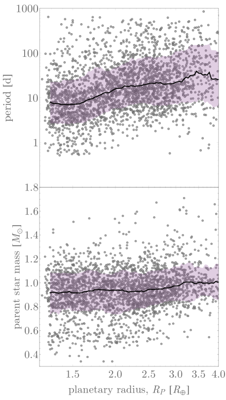
Figure 2: Orbital periods (top) and host star masses (bottom) as a function of planetary radius for the 2936 KOIs with modal class probability of being Neptunian and not dispositioned as a false-positive on NEA. The trend between period and radius is most easily explained as being due to detection bias, which in turn gives rise to the RV plateau seen for the Neptunians in Figure 1. Median (black line) and 68.3% credible interval (purple) shown using a top-hat smoothing kernel of 0.14 dex.

Figure 2 reveals that there is indeed an apparent trend between planetary radius and orbital period for the Kepler Neptunes, which is most easily explained as being due to detection bias. We find no such trend for stellar mass, although Kepler had a strong selection bias towards Solar-like stars and thus the sample is limited for low-mass stars.

3.3 Promising Small Planets for RV follow-up

We here demonstrate perhaps the most useful application of this work, for identifying promising small planets for RV follow-up. In this work, we have applied forecaster to Kepler planets but this should be treated as a demonstration of what could be done with the upcoming TESS survey too (Ricker et al., 2015). In particular, the narrow-but-deep nature of Kepler combined with the fact RV amplitudes are enhanced for low-mass star means that the most favorable targets (in terms of absolute RV amplitude) will be around faint stars. The all-sky nature of TESS will lead to brighter targets and here forecaster can clearly play a direct role in identifying promising follow-up targets.

Table 3: List of planetary candidates with maximum likelihood radii between 0.5 to 4.0 Earth radii and unusually high forecasted RV semi-amplitudes.

KOI	$R_{P}$ $[R_{\oplus}]$	$K$ $[\mathrm{m/s}]$	$M_{\star}$ $[M_{\odot}]$	$P_{P}$ $[\mathrm{days}]$	$K_{P}$
0596.01	$1.29_{-0.14}^{+0.12}$	$1.82_{-0.62}^{+1.42}$	$0.485_{-0.045}^{+0.039}$	$1.6827$	14.818
0739.01	$1.45_{-0.10}^{+0.10}$	$2.57_{-0.87}^{+1.90}$	$0.533_{-0.037}^{+0.033}$	$1.2871$	15.488
0936.02	$1.29_{-0.14}^{+0.12}$	$2.29_{-0.78}^{+1.78}$	$0.479_{-0.049}^{+0.039}$	$0.8930$	15.073
0952.05	$1.38_{-0.12}^{+0.13}$	$2.88_{-1.02}^{+2.13}$	$0.506_{-0.041}^{+0.037}$	$0.7430$	15.801
0961.01	$0.81_{-0.12}^{+0.16}$	$0.98_{-0.45}^{+0.93}$	$0.144_{-0.022}^{+0.030}$	$1.2138$	15.920
0961.02	$0.87_{-0.13}^{+0.15}$	$1.78_{-0.80}^{+1.77}$	$0.144_{-0.022}^{+0.030}$	$0.4533$	15.920
1202.01	$1.23_{-0.08}^{+0.09}$	$1.74_{-0.56}^{+1.28}$	$0.614_{-0.029}^{+0.030}$	$0.9283$	15.854
1300.01	$1.12_{-0.10}^{+0.08}$	$1.58_{-0.54}^{+1.17}$	$0.540_{-0.034}^{+0.034}$	$0.6313$	14.285
1367.01	$1.55_{-0.07}^{+0.11}$	$2.95_{-1.05}^{+2.06}$	$0.840_{-0.039}^{+0.037}$	$0.5679$	15.055
1880.01	$1.35_{-0.12}^{+0.20}$	$2.29_{-0.81}^{+1.78}$	$0.553_{-0.031}^{+0.030}$	$1.1512$	14.440
2119.01	$1.35_{-0.06}^{+0.10}$	$2.14_{-0.73}^{+1.66}$	$0.849_{-0.038}^{+0.039}$	$0.5710$	14.098
2250.02	$1.66_{-0.15}^{+0.12}$	$3.24_{-1.15}^{+2.39}$	$0.812_{-0.059}^{+0.055}$	$0.6263$	15.622
2347.01	$1.00_{-0.07}^{+0.07}$	$1.05_{-0.36}^{+0.81}$	$0.580_{-0.030}^{+0.029}$	$0.5880$	14.934
2393.02	$1.23_{-0.08}^{+0.09}$	$1.58_{-0.51}^{+1.17}$	$0.790_{-0.036}^{+0.031}$	$0.7667$	14.903
2409.01	$1.55_{-0.14}^{+0.19}$	$3.09_{-1.10}^{+2.28}$	$0.764_{-0.065}^{+0.080}$	$0.5774$	14.859
2480.01	$1.35_{-0.12}^{+0.16}$	$2.63_{-0.89}^{+2.16}$	$0.558_{-0.048}^{+0.050}$	$0.6668$	15.745
2493.01	$1.55_{-0.14}^{+0.19}$	$2.75_{-0.98}^{+2.14}$	$0.844_{-0.068}^{+0.066}$	$0.6631$	15.304
2699.01	$1.62_{-0.14}^{+0.20}$	$3.16_{-1.17}^{+2.33}$	$0.853_{-0.077}^{+0.065}$	$0.5689$	15.230
2704.01	$2.40_{-0.58}^{+0.62}$	$7.41_{-3.15}^{+6.08}$	$0.189_{-0.050}^{+0.068}$	$4.8712$	17.475
2704.02	$1.55_{-0.37}^{+0.45}$	$4.07_{-1.67}^{+3.69}$	$0.189_{-0.050}^{+0.068}$	$2.9842$	17.475
2735.01	$1.48_{-0.13}^{+0.18}$	$2.69_{-0.95}^{+2.09}$	$0.864_{-0.063}^{+0.054}$	$0.5588$	15.600
2783.01	$0.65_{-0.06}^{+0.05}$	$0.23_{-0.08}^{+0.14}$	$0.518_{-0.032}^{+0.030}$	$0.5269$	14.694
2793.02	$1.48_{-0.16}^{+0.14}$	$2.63_{-0.93}^{+2.05}$	$0.456_{-0.046}^{+0.043}$	$1.7668$	16.283
2817.01	$1.55_{-0.17}^{+0.19}$	$2.82_{-1.04}^{+2.19}$	$0.805_{-0.074}^{+0.076}$	$0.6340$	15.760
2842.01	$1.95_{-0.21}^{+0.24}$	$5.50_{-2.18}^{+4.05}$	$0.343_{-0.047}^{+0.044}$	$1.5654$	16.257
2842.03	$1.58_{-0.17}^{+0.19}$	$3.09_{-1.10}^{+2.28}$	$0.343_{-0.047}^{+0.044}$	$3.0362$	16.257
3119.01	$1.20_{-0.16}^{+0.18}$	$2.14_{-0.82}^{+1.75}$	$0.249_{-0.036}^{+0.045}$	$2.1844$	16.946
4002.01	$1.38_{-0.09}^{+0.13}$	$2.24_{-0.76}^{+1.74}$	$0.883_{-0.042}^{+0.044}$	$0.5242$	15.040

We list 28 promising targets in Table 3, where we haved down-selected on KOIs not dispositioned as false-positives on NEA, with radii between one half to four times that of the Earth and with unusually high RV amplitude predictions. For the latter criteria, we specifically used $\hat{K}-K_{\mathrm{med}}>1.64(\hat{K}-K_{\mathrm{lower}})$, where $\hat{K}$ is the median forecast for $K$, $K_{\mathrm{lower}}$ is the 15.9% lower quantile of the forecasted $K$ distribution and $K_{\mathrm{med}}$ is the running median of the median forecasts of $K$ with the same window size as used before (note that $1.64$ $\sigma=90$%). These KOIs are visualized versus the ensemble of small KOIs in Figure 3.

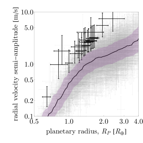
Figure 3: Forecasted radial velocity amplitudes for small planets. The colored region contains the 68.3% credible interval of maximum likeihood forecasted $K$ values from a moving window. Points plotted use 68.3% uncertainties and the black points are those more than 1.64 $\sigma$ (90%) above the moving median (black).

As can be seen from Table 3, this sample of 28 KOIs all have Kepler-bandpass magnitudes fainter than $K_{P}>14$. The 1.35 $R_{\oplus}$ planetary candidate KOI-2119.01 is brightest at $K_{P}=14.1$, for which we predict a $\sim 2$ m/s amplitude. This sample of targets also highlights the great potential of near-infrared spectrographs (e.g. Cersullo et al. 2017), where the apparent magnitude is significantly brighter.

Despite their faintness, the very short-period nature of these objects (as evident from Table 3) enables repeat monitoring and potentially easier disentanglement of spurious signals originating from the star (Pepe et al., 2013; Howard et al., 2013). Thus, despite the challenges, these targets may be worth pursueing for Kepler and indeed one can expect this approach to yield far more suitable targets in the TESS-era.

4 Discussion

In this work, we have used a data-driven and probabilistic mass-radius relation to forecast the masses of approximately seven thousands KOIs with careful attention to correctly propagate parameter covariances and uncertainties (see Wolfgang & Rogers & Ford 2016 and Chen & Kipping 2017). We report 1 and 2 $\sigma$ credible intervals for each KOI in Table 2, including derived parameters such as density, surface gravity and radial velocity semi-amplitude. Full joint posterior samples are made publicly available at this URL(https://github.com/chenjj2/forecasts). We stress that these results should be treated as informed, probabilistic and model-conditioned predictions and not measurements.

forecaster has already seen numerous applications (e.g. see Foreman-Mackey et al. 2016; Obermeier et al. 2016; Dressing et al. 2017; Rodriguez et al. 2017) to individual systems or small subsets, but we believe this to be the first application to a large (several hundred) ensemble of planets ensuring homogeneous methodology. This work serves as a demonstration of ensemble predictions for planetary masses based off transit-derived radii. In the near-future, one can expect the number of planetary candidates discovered through transits to continue to rapidly grow, exacerbating the demands on follow-up resources, for which planetary mass is frequently a key driver for various observational signatures (e.g. radial velocities, atmospheric scale heights, ring/moon stability). For example, TESS is expected to discover $\sim 5,000$ transiting planets (Bouma et al., 2017), LSST a further $\sim\mathcal{O}[10^{3}]$-$\mathcal{O}[10^{4}]$ (Lund et al., 2015) and $\sim\mathcal{O}[10^{4}]$ from PLATO (Rauer et al., 2014). In choosing the subset of targets for follow-up, forecasted masses will frequently be beneficial, and thus the analysis provided in this work can be considered as a template for these future surveys too.

As an example, we have shown how this approach can quickly identify small KOIs for which the radial velocity amplitudes are unusually high, increasing the chances for detection (see Section 3.3). The combination of their forecasted mass, low parent star mass and short orbital period maximizes $K$. However, the deep-sky nature of Kepler, and the bias towards low-mass stars, means these targets are faint - a problem likely to be resolved with the all-sky surveys of TESS and PLATO. Of course, realistic target selection will depend upon more than just signal amplitude, likely factoring in expected noise, planet properties and other program-specific questions of interest (e.g. see Kipping & Lam 2017 for an example of target selection based on forecasted multiplicity).

Future improvements to the forecasts made in this work are unlikely to result from simply obtaining more precise planetary radii, since the predicted mass uncertainties are observed to be dominated by the intrinsic dispersion inherent to the model itself (see Section 3.2). Future work could attempt to build an updated probabilistic model using more data and likely a second dependent variable, such as insolation for example. Until that time, the forecasts made here are likely the most credible estimates available without direct observation.

References

- Agol et al. (2005) Agol, E., Steffen, J., Sari, R. & Clarkson, W. 2005. MNRAS 359, 567.
- Akeson et al. (2013) Akeson, R. L. et al. 2013. PASP 125, 989.
- Barnes & O’Brien (2002) Barnes, J. W. & O’Brien, D. P. 2002. ApJ 575, 1087.
- Bouma et al. (2017) Bouma, L. G., Winn, J. N., Kosiarek, J. & McCullough, P. R. 2017. arXiv e-prints: 1705.08891
- Carter et al. (2008) Carter, J. A., Yee, J. C., Eastman, J., Gaudi, B. S. & Winn, J. N. 2008. ApJ 689, 499.
- Cersullo et al. (2017) Cersullo, F., Wildi, F., Chazelas, B. & Pepe, F. 2017. A&A 601, 102.
- Chen & Kipping (2017) Chen, J. & Kipping, D. M. 2017. ApJ 834, 17.
- Coughlin et al. (2016) Coughlin, J. L. et al. 2016. ApJS 224, 27.
- Dotter et al. (2008) Dotter, A., Chaboyer, B., Jevremović, D., Kostov, V., Baron, E. & Ferguson, J. W. 2008. ApJS 178, 89.
- Dressing et al. (2017) Dressing, C. D. et al. 2017. arXiv e-prints: 1703.07416
- Foreman-Mackey et al. (2016) Foreman-Mackey, D., Morton, T. D., Hogg, D. W., Agol, E. & Schölkopf, B. 2016. ApJ 152, 206.
- Foreman-Mackey et al. (2016) Foreman-Mackey, D., Morton, T. D., Hogg, D. W., Agol, E. & Schölkopf, B. 2016. arXiv e-prints: 1607.08237
- Hatzes & Rauer (2015) Hatzes, A. P. & Rauer, H. 2015. ApJ 810, 25.
- Heng & Vogt (2011) Heng, K. & Vogt, S. S. 2011. MNRAS 415, 2145.
- Holman & Murray (2005) Holman, M. J. & Murray, N. W. 2005. Science 307, 1288.
- Howard et al. (2013) Howard, A. W. et al. 2013. Nature 503, 381.
- Jacob (1855) Jacob, W. S. 1855. MNRAS 15, 228.
- Johnson et al. (2017) Johnson, J. A. et al. 2017. AAS Journals, submitted (arXiv e-prints:1703.10402)
- Kipping (2009a) Kipping, D. M. 2009a. MNRAS 392, 181.
- Kipping (2009b) Kipping, D. M. 2009a. MNRAS 396, 1797.
- Kipping & Sandford (2016) Kipping, D. M. & Sandford, E. 2016. MNRAS 463, 1323.
- Kipping et al. (2017) Kipping, D. M. et al. 2016. ApJ 820, 112.
- Kipping & Lam (2017) Kipping, D. M. & Lam, C. 2017. MNRAS 465, 3495.
- Kopal (1959) Kopal, Z. 1959. The International Astrophysics Series: Close binary systems, London: Chapman & Hall.
- Lund et al. (2015) Lund, M. B., Pepper, J. & Stassun, K. G. 2015. AJ 149, 16.
- Mandel & Agol (2002) Mandel, K. & Agol, E. 2002. ApJ 580, L171.
- Mathur et al. (2017) Mathur, S. et al. 2017. ApJS 229, 30.
- Millis & Mazeh (2017) Millis, S. M. & Mazeh, T. 2017. ApJ 839, 8.
- Pepe et al. (2013)
- Obermeier et al. (2016) Obermeier, C. et al. 2016. arXiv e-prints: 1608.04760 Pepe, F. et al. 2013. Nature 503, 377.
- Rauer et al. (2014) Rauer, H. 2014. Exp. Astron. 38, 249
- Ricker et al. (2015) Ricker, G. R. et al. 2015,. SPIE Journal of Astronomical Telescopes, Instruments, and Systems, 1, 014003.
- Rodriguez et al. (2017) Rodriguez, J. E. et al. 2017. arXiv e-prints: 1701.03807
- Rowe & Thompson (2015) Rowe, J. & Thompson, S. E. 2015. arXiv e-prints: 1504.00707.
- Rybicki & Lightman (1979) Rybicki, G. B, & Lightman, A. P. 1979. Radiative Processes in Astrophysics (New York: Wiley)
- Seager & Sasselov (2000) Seager, S. & Sasselov, D. D. 2000. ApJ 537, 916.
- Schlichting & Chang (2011) Schlichting, H. E. & Chang, P. 2011. ApJ 734, 117.
- Steffen (2016) Steffen, J. H. 2016. MNRAS, 457, 4384.
- Struve (1952) Struve, O. 1952. The Observatory 72, 199.
- Weiss & Marcy (2014) Weiss, L. M. & Marcy, G. W. 2014. ApJ 783, 6.
- Wolfgang & Rogers & Ford (2016) Wolfgang, A. & Rogers, L. A. & Ford, E. B. 2016. ApJ 825, 19.
- Zuluaga et al. (2015) Zuluaga, J. I., Kipping, D. M., Sucerquia, M., Alvarado, J. A. 2015. ApJ 803, 14