The chemical composition of the stellar cluster Gaia1:
no surprise behind Sirius

We observed 6 He-clump stars of the intermediate-age stellar cluster Gaia1 with the MIKE/MAGELLAN spectrograph. A possible extra-galactic origin of this cluster, recently discovered thanks to the first data release of the ESA Gaia mission, has been suggested, based on its orbital parameters. Abundances for Fe, $\alpha$, proton- and neutron-capture elements have been obtained. We find no evidence of intrinsic abundance spreads. The iron abundance is solar ([FeI/H]=+0.00 $\pm 0.01$; $\sigma=0.03$ dex). All the other abundance ratios are, by and large, solar-scaled, similar to the Galactic thin disk and open clusters stars of similar metallicity. The chemical composition of Gaia1 does not support an extra-galactic origin for this stellar cluster, that can be considered as a standard Galactic open cluster.

1 Introduction

Gaia1 is a stellar cluster that has been recently identified by Koposov, Belokurov & Torrealba (2017) using the first data release of the ESA Gaia mission (Brown et al. 2016). Its identification has been precluded for decades by its proximity ($\sim 10$ arcmin) to the bright star Sirius.

Recently, Simpson et al. (2017, hereafter S17) performed a prompt spectroscopic follow-up of this system, confirming that Gaia1 is a stellar cluster, according to its radial velocity (RVs) and [Fe/H]. They identified 41 cluster members, 27 of them observed with the high-resolution spectrograph HERMES and the other ones with the low-resolution spectrograph AAOmega, both at the Anglo-Australian Telescope. The mean radial velocity is +58.30$\pm$0.22 km/s, with a dispersion of 0.94$\pm$0.15 km/s, while the mean iron abundance (from HERMES targets only) is [Fe/H]=–0.13$\pm$0.13 dex and its age is $\sim$3 Gyr. Using Gaia and 2MASS positions for the cluster stars, they derived a first estimate of its proper motion and of its orbit, in particular finding a Galactocentric distance ($R_{GC}$) of 11.8$\pm$0.2 kpc, a maximum height above the Galactic plane of $z_{max}=1.7^{+2.1}_{-0.9}$ kpc and an eccentricity $\epsilon=0.3\pm 0.2$. These orbital parameters, taken at face values, could suggest an extra-galactic origin for Gaia1, even if they have large uncertainties that prevent any firm conclusion.

In this paper we present chemical abundances of Fe, Na, Mg, Al, Si, Ca, Ti, Ba and Eu for 6 giant stars observed at the Magellan II Telescope.

2 Observations

Spectra of 7 stars having infrared colors and magnitudes compatible with being He-clump stars of the stellar cluster Gaia1 have been secured using the Magellan Inamori Kyocera Echelle (MIKE) spectrograph (Bernstein et al. 2003) mounted on the Magellan II Telescope at Las Campanas Observatory. Table 3 lists the coordinates, the 2MASS magnitudes, RVs and atmospheric parameters for the observed targets. The position of the observed targets in the 2MASS ($K_{S}$ vs (J-$K_{S}$)) color-magnitude diagram is shown in left-upper panel of Fig. 1 as red points. Left-lower panel shows (as blue points) the position of the targets observed with HERMES by S17. All the MIKE targets have been observed with the 0.7” x 5.0” slit, providing a spectral resolution of $\sim$36000 in the red arm (covering from $\sim$5000 to $\sim$9150 Å ). Exposure times varied from 600 to 1800 sec. The signal-to-noise ratio ranges from $\sim$40 to $\sim$80 at $\sim$6000 Å . Bias-subtraction, flat-fielding, spectral extraction and wavelength calibration have been performed using the CarPy MIKE pipeline (Kelson 2003).

RVs have been measured through DAOSPEC (Stetson & Pancino 2008) by measuring the position of almost 400 metallic and unblended lines selected in the red spectrum. Six among the target stars share very similar RVs (see Table 3) and are classified as members of Gaia1. Star #3, instead, presents a different RV and damped absorption lines, and is, as such, considered not member and will not be further discussed. The mean heliocentric RV is +57.6$\pm$0.4 km/s ($\sigma$= 1.0 km/s) that nicely matches with the value derived by S17.

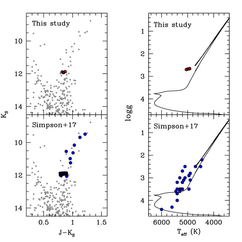
Figure 1: Left panels: the 2MASS ($K_{S}$ vs (J-$K_{S}$)) color-magnitude diagram of Gaia1 (grey points) with marked the position of our targets (red points) and of those by S17 (blue points). Right panels: position of the MIKE and HERMES targets in the $T_{eff}$–log g plane, superimposed to a theoretical isochrone by Bressan et al. (2012) with [Fe/H]= 0.0 and age 3 Gyr. Unexpectedly, the S17 stars do not define an RGB in the theoretical plane, suggesting that their parameters are not correct.

Table 1: Main information on the observed MIKE targets: 2mass identification number, 2MASS J and $K_{S}$ magnitudes, RV and atmospheric parameters derived from the MIKE spectra, together with the SNR measured at $\sim$600nm.

ID	ID2MASS	RAJ2000	DecJ2000	J	$K_{S}$	RV	Teff	log g	vt	SNR
		[deg]	[deg]			[km/s]	[oK]	[cm s-2]	[km/s]	@600nm
1	2MASS06455819-1641596	101.492499	-16.699909	12.731	11.860	+58.2	5000$\pm$60	2.68$\pm$0.10	1.5$\pm$0.1	60
2	2MASS06454837-1643113	101.451559	-16.719822	12.782	11.932	+58.4	4960$\pm$80	2.67$\pm$0.12	1.5$\pm$0.1	40
3	2MASS06454801-1642240	101.450069	-16.706678	12.832	11.996	+64.5	—	—	—	40
4	2MASS06455237-1643471	101.468234	-16.729773	12.698	11.878	+57.2	5050$\pm$80	2.70$\pm$0.12	1.4$\pm$0.1	40
5	2MASS06455379-1645521	101.474151	-16.764490	12.770	11.930	+57.4	4960$\pm$60	2.67$\pm$0.10	1.4$\pm$0.1	70
6	2MASS06460723-1647294	101.530159	-16.791500	12.753	11.913	+56.0	4920$\pm$50	2.66$\pm$0.10	1.3$\pm$0.1	80
7	2MASS06455253-1640582	101.468910	-16.682854	12.758	11.918	+58.5	4960$\pm$50	2.67$\pm$0.10	1.6$\pm$0.1	80

3 Chemical analysis

3.1 Atmospheric parameters

The atmospheric parameters have been derived as follows: (i) effective temperatures ($T_{eff}$) have been derived spectroscopically from the excitation equilibrium thanks to the large number ($\sim$120) of measured Fe I lines; (ii) surface gravities (log g) have been obtained from the Stefan-Boltzmann relation, adopting the spectroscopic $T_{eff}$, the bolometric corrections calculated according to Buzzoni et al. (2010), the true distance modulus $(m-M)_{0}$= 13.3 (S17 from the 2MASS photometry) and the color excess E(B-V)= 0.41 mag obtained from the maps by Schlegel, Finkbeiner & Davis (1998) corrected according to Bonifacio, Monai & Beers (2000). For all the stars a stellar mass of 1.5 $M_{\odot}$ has been adopted; (iii) microturbulent velocities (v_t) have been obtained by minimizing the trend between iron abundance and line strength.

The advantage of this hybrid approach is to exploit at the best all the information in hand, both from spectroscopy and photometry, and to minimize the uncertainties in the color excess that affect mainly the photometric $T_{eff}$, as well as possible systematics in the ionization equilibrium due to over-ionization effects that affect the spectroscopic log g.

Right-upper panel of Fig. 1 shows the position of the observed targets in the $T_{eff}$-log g plane (red points) in comparison with a theoretical isochrone from Padua database (Bressan et al. 2012) with solar metallicity and an age of 3 Gyr (see S17). We find that within the uncertainties the atmospheric parameters (derived as explained above) reasonably fit the position expected for the He-clump. On the other hand, an inspection on the atmospheric parameters derived by S17 for their targets reveals a significant discrepancy with the atmospheric parameters expected for their evolutionary stage (right-lower panel of Fig. 1). Even if their observed targets belong to the He-clump or to the bright red giant branch, $T_{eff}$ and log g are compatible with those of less evolved stars. In particular, half of their sample (14 out 27 stars) have log g higher than 3.5, that are values unlikely for the observed targets and a systematic offset toward higher $T_{eff}$ seems to be present, with the extreme case of a He-clump star for which they estimated $T_{eff}$= 6000 K and log g= 4.4. Note that S17 derived all the atmospheric parameters spectroscopically: we stress that this approach can be very dangerous in case of low-quality spectra and/or when the number of Fe lines are not large enough to guarantee a robust coverage in excitation potential and line strength, or when the Fe II lines are too few/too weak.

3.2 Sanity check

As a sanity check we derived the atmospheric parameters using different methods. First, $T_{eff}$ and log g have been derived from the photometry, adopting the $(J-K)_{0}$-$T_{eff}$ transformation by Gonzalez Hernandez & Bonifacio (2009). The photometric $T_{eff}$ are on average lower than spectroscopic ones by $\sim$200-300 K. However, a significant (at a level of 3-5 $\sigma$) positive slope between iron abundances and excitation potential is found for all the targets, pointing out that the photometric $T_{eff}$ are not totally correct, probably due to the large uncertainties in the color excess. The use of photometric parameters leads to a decrease of [Fe/H] of about 0.2 dex. On the other hand, a fully spectroscopic determination of all the parameters provides $T_{eff}$ very similar to that obtained above and log g higher by $\sim$0.3, but with a negligible impact on the abundance ratios discussed here.

3.3 Abundance determination

Abundances for Fe, Na, Al, Si, Ca and Ti have been derived from the equivalent widths of unblended transitions (measured with the code DAOSPEC) and using the code GALA (Mucciarelli et al. 2013a) based on the suite of software developed by R. L. Kurucz. Abundances for Mg, Ba and Eu have been derived from spectral synthesis, because the used Mg lines ($\sim$6318-19 Å ) are located on the red wing of an auto-ionization Ca line, while the Ba and Eu lines are affected by isotopic and hyperfine splittings. Solar reference abundances are from Grevesse & Sauval (1998). The linelist and the determination of the abundances uncertainties are described in Appendix A and B, respectively.

Table 2: Measured chemical abundance ratios for individual MIKE targets. Last row lists the mean abundances and the corresponding 1$\sigma$ uncertainty.

ID	[FeI/H]	[Na/Fe]	[Mg/Fe]	[Al/Fe]	[Si/Fe]	[Ca/Fe]	[Ti/Fe]	[BaII/Fe]	[EuII/Fe]
1	-0.02$\pm$0.07	–0.14$\pm$0.05	+0.02$\pm$0.04	+0.13$\pm$0.05	+0.01$\pm$0.07	–0.03$\pm$0.05	+0.02$\pm$0.06	+0.26$\pm$0.10	–0.04$\pm$0.06
2	+0.05$\pm$0.06	–0.02$\pm$0.07	–0.02$\pm$0.07	+0.01$\pm$0.10	+0.03$\pm$0.08	–0.06$\pm$0.06	–0.01$\pm$0.06	+0.14$\pm$0.08	+0.00$\pm$0.08
4	-0.02$\pm$0.07	–0.13$\pm$0.10	+0.09$\pm$0.07	+0.08$\pm$0.07	–0.02$\pm$0.08	–0.08$\pm$0.03	+0.00$\pm$0.05	+0.21$\pm$0.05	–0.06$\pm$0.08
5	+0.00$\pm$0.06	–0.08$\pm$0.05	+0.00$\pm$0.05	+0.13$\pm$0.04	–0.01$\pm$0.07	–0.09$\pm$0.04	–0.04$\pm$0.07	+0.23$\pm$0.10	+0.15$\pm$0.06
6	+0.01$\pm$0.06	–0.08$\pm$0.06	+0.06$\pm$0.07	+0.07$\pm$0.05	+0.03$\pm$0.08	–0.04$\pm$0.07	–0.04$\pm$0.07	+0.22$\pm$0.11	+0.10$\pm$0.07
7	-0.03$\pm$0.06	–0.02$\pm$0.06	+0.11$\pm$0.07	+0.11$\pm$0.04	–0.03$\pm$0.07	–0.01$\pm$0.05	+0.02$\pm$0.06	+0.15$\pm$0.11	+0.07$\pm$0.07
Mean ($\sigma$)	+0.00 (0.03)	–0.08 (0.05)	+0.04 (0.05)	+0.09 (0.04)	+0.00 (0.03)	–0.05 (0.03)	–0.01 (0.03)	+0.20 (0.05)	+0.04 (0.08)

4 The chemical composition of Gaia1

4.1 Iron content

Gaia1 has an average iron abundance of [FeI/H]=+0.00$\pm$0.01 dex ($\sigma$= 0.03 dex). We used the maximum likelihood (ML) algorithm described in Mucciarelli et al. (2012) to estimate whether the observed scatter is compatible or not with a null intrinsic spread, taking into account the uncertainties of individual stars. The observed [FeI/H] spread turns out to be fully consistent with a null intrinsic spread. The same conclusions are obtained adopting the pure spectroscopic and photometric sets of atmospheric parameters. The former set of parameters provides a very similar abundance, while the latter one provides an average abundance lower by $\sim$0.2 dex because of the lower $T_{eff}$.

S17 derived from 27 giant stars observed with HERMES an average abundance [Fe/H]=–0.13$\pm$0.03 dex ($\sigma$= 0.13 dex). Using their quoted uncertainties, the ML algorithm suggests the presence of a non-null intrinsic spread, $\sigma_{int}$= 0.12$\pm$0.01 dex, at variance to our analysis. Even if their sample is significantly larger than ours, the intrinsic iron spread obtained from their abundances is likely due to two effects: (1) the large uncertainty in their spectroscopic parameters (see Fig. 1), and (2) the fact that their [Fe/H] uncertainties do not include the contribution of the atmospherical parameters errors, hence under-estimating the total errorbar. Even if the metallicities derived by S17 and in this study are consistent, we discourage the use of their atmospheric parameters that turn out to be inconsistent with the evolutionary stages of the observed stars.

4.2 $\alpha$-elements

The measured [$\alpha$/Fe] abundance ratios (see Table 2) turn out to be solar-scaled, pointing out that the cluster formed from a gas enriched both from Type II and Type Ia supernovae. Fig. 2 shows the behaviour of the measured [$\alpha$/Fe] abundance ratios as a function of [Fe/H] in comparison with the Galactic thin disk stars (grey points, Soubiran & Girard 2005). For all the abundance ratios, Gaia1 well matches the mean locus described by the Galactic field stars, suggesting a strong similarity with the Galactic thin disk.

4.3 Na and Al

Na and Al are usually associated to nucleosynthesis by proton-captures. We derived for Gaia1 [Na/Fe]=–0.08$\pm$0.02 ($\sigma$=0.05 dex) and [Al/Fe]=+0.09$\pm$0.02 ($\sigma$=0.05 dex). As visible in the upper panels of Fig. 3, at the same metallicity of the cluster the thin disk stars are essentially solar-scaled and Gaia1 well matches, for both the abundance ratios, the observed Galactic trend. Note that [Na/Fe] values shown in Fig. 3 for Galactic stars do not include corrections for non-local thermodynamical equilibrium. In order to provide a homogeneous comparison with the literature data for the thin disk stars, we did not taken into account such corrections in our measured [Na/Fe]. However, corrections for the targets estimated according to Lind et al. (2011) are of about –0.1 dex and they do not change significantly our conclusions.

No evidence of intrinsic Na and Al star-to-star scatters is found for these stars. Such chemical inhomogeneities are commonly observed among globular cluster stars (see Gratton, Carretta & Bragaglia 2012, and references therein) and usually explained within a framework of a self-enrichment process. On the other hand, open cluster stars, in virtue of their lower mass and density, do not undergo to self-enrichment processes and they show homogeneous Na and Al contents. The lack of significant star-to-star variations in Gaia1 (despite the small number of observed stars) agrees with its current low mass ($\sim 10^{4}M_{\odot}$ Koposov, Belokurov & Torrealba 2017). It is also likely that the cluster suffered only limited mass loss in the $\sim$3 Gyr that elapsed since its formation.

4.4 Neutron-capture elements: Ba and Eu

We measured Ba, as prototype of elements produced through slow neutron captures, and Eu, mainly produced through rapid neutron captures, obtaining [Ba/Fe]=+0.20$\pm$0.02 ($\sigma$= 0.05 dex) and [Eu/Fe]=+0.04$\pm$0.03 ($\sigma$= 0.08 dex), respectively. Lower-panels of Fig. 3 show the behaviour of [Ba/Fe] and [Eu/Fe] abundance ratios measured in Gaia1: also for these two elements we find a good agreement with the Galactic thin disk stars of similar metallicity.

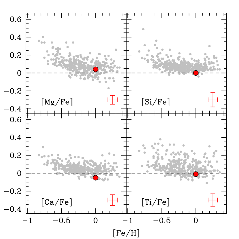
Figure 2: The behaviour of the average [Mg/Fe], [Si/Fe], [Ca/Fe] and [Ti/Fe] abundance ratios of Gaia1 as a function of [Fe/H] (red point), in comparison with Galactic thin disk stars (grey points, Soubiran & Girard 2005)

.

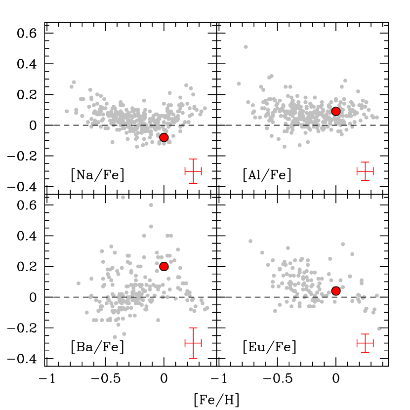
Figure 3: The behaviour of the average [Na/Fe], [Al/Fe], [Ba/Fe] and [Eu/Fe] abundance ratios of Gaia1 as a function of [Fe/H] (red point), in comparison with Galatic thin disk stars (grey points, Soubiran & Girard (2005) for Na and Al, and Reddy et al. (2003); Bensby et al. (2005) for Ba and Eu)

.

5 Conclusions

The chemical composition of Gaia1 that we derived from MIKE spectra well matches with that of thin disk stars and open clusters with similar metallicity (see e.g. Pancino et al. 2010; Mishenina et al. 2015, and reference therein). This nice match has been found for all the main groups of elements, i.e. $\alpha$, proton- and neutron-capture elements, indicating that this cluster formed from a gas that has had a chemical enrichment similar to that of the Galactic thin disk. A possible extra-galactic origin of Gaia1 is not supported by the comparison between its chemical composition and that of other stellar systems. The galaxies currently populating the Local Group are more metal-poor than Gaia1 and they do not reach solar metallicity (McConnachie 2012). The only extra-galactic environment approaching similar metallicities is the Sagittarius dwarf spheroidal galaxy but its most metal-rich stars are characterized by sub-solar [$\alpha$/Fe] abundance ratios and enhanced [Ba/Fe] and [Eu/Fe] (Bonifacio et al. 2000; Monaco et al. 2005; Sbordone et al. 2007).

The mean metallicity of the thin disk (both field and open cluster stars) is known to decrease at large galactocentric distances (Pancino et al. 2010; Hayden et al. 2015; Netopil et al. 2016; Magrini et al. 2017). As shown in Fig. 4, at the distance of Gaia1, the mean metallicity of open clusters is about –0.3 dex lower than that of the cluster, even if a large dispersion is observed at these distances. Solar metallicity open clusters are typically found at $R_{GC}$ of $\sim$7-8 kpc. On the other hand, stars with solar metallicity are present in the thin disk also at similar distances: the metallicity distribution for thin disk stars provided by Hayden et al. (2015) at 11$<R_{GC}<$13 kpc and 1$<\mid{z}\mid<$2 kpc is peaked at [Fe/H]=–0.38 dex but reaching super-solar metallicities.

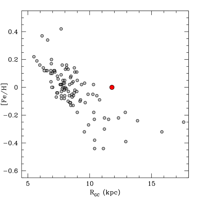
Figure 4: The behaviour of [Fe/H] as a function of the Galactocentric distance for open clusters (Netopil et al. 2016; Magrini et al. 2017, grey circles) and Gaia1 (red point).

Our results on the chemical composition strongly argue against an extra-galactic origin for Gaia1. In fact it appears to be an unremarkable standard Galactic open cluster. Its position with respect to the overall trend between [Fe/H] and $R_{GC}$ could suggest that it formed in the inner disk, progressively migrating toward higher $R_{GC}$, thus explaining its possible peculiar orbit with respect to other open clusters. However, it is worth noticing that the precise value of $R_{GC}$ can be affected by the value of E(B-V) that remains still uncertain for this cluster. We checked the measured abundance ratios with those derived by Nissen et al. (2016) for solar twin stars of ages similar to that of Gaia1 in the solar neighborhood. Within the uncertainties the abundances of Gaia1 are comparable with those of the solar neighborhood, but for [Al/Fe] and [Ba/Fe] that in this cluster are higher (by $\sim$0.1 dex) with respect to coeval solar twin stars. However, we cannot totally rule out that Gaia1 originally formed in the solar neighborhood.

Although the orbital parameters inferred by S17 may suggest that the cluster has been accreted by the Milky Way, they are still, within uncertainties, fully compatible with the majority of known Galactic open clusters. The uncertainty on the orbit of Gaia1 is dominated by the uncertainty on its proper motion. The situation will be greatly improved with the second Gaia data release, and we defer any conclusion on its kinematics to that time.

Appendix A Linelist

The analysed lines have been selected according to a synthetic spectrum calculated with the code SYNTHE, adopting a model atmosphere calculated with ATLAS9 with the representative atmospheric parameters of the stars (that have $T_{eff}$, log g and $v_{t}$ very similar each other). The reference synthetic spectrum has been computed including all the atomic and molecular transitions of the last version of the Kurucz/Castelli linelists, updating the oscillator strengths for some transitions of interest (as explained below). For the abundances calculated using the equivalent widths (EW) we selected only lines predicted to be unblended. Atomic data for Fe I lines are from Martin, Fuhr & Wiese (1998) and Fuhr & Wiese (2006), while those for Fe II lines from Melendez & Barbuy (2009). Oscillator strengths for Ca I lines are mainly from Smith & Raggett (1981), for Ti I lines are from Martin, Fuhr & Wiese (1998) and Lawler et al. (2013). For Si I lines we adopted, when available, the furnace oscillator strengths by Garz (1973), while for other lines, for which the available log gf have large uncertainties or badly reproduce the solar spectrum, we derived astrophysical oscillator strengths using the solar flux spectra of Neckel & Labs (1984) and a solar model atmosphere calculated with the chemical mixture of Grevesse & Sauval (1998). The same method has been adopted to compute the oscillator strengths for the Al I doublet at 6696-6698 Å because the available values in literature underestimate the solar abundance of about 0.2 dex. For the two used Na I doublets at 5682-88 Å and 6154-6160 Å we employed the log gf available in the NIST database, as well as for the Mg I doublet at 6318-6319 Å . For the transitions measured using spectral synthesis because affected by hyperfine and isotopic splitting, we adopted the linelists available in the Kurucz/Castelli database (Ba II lines) and that provided by Lawler et al. (2001) (Eu II line). Table A.1 lists for all the used lines the measured EW and the adopted oscillator strength and excitation potential.

Table 3: Wavelength, oscillator-strength, excitation potential and measured EW for the used transitions. The complete version of the table is available in electronic form.

ID	$\lambda$	Element	log gf	$\chi$	EW
	(Å )			(eV)	(mÅ )
1	5197.9	26.00	-1.620	4.300	45.30
1	5236.2	26.00	-1.497	4.190	71.10
1	5249.1	26.00	-1.460	4.470	47.60
1	5315.1	26.00	-1.550	4.370	55.10
1	5326.8	26.00	-2.100	4.410	25.60
1	5379.6	26.00	-1.514	3.690	83.20
1	5386.3	26.00	-1.740	4.150	45.90
1	5398.3	26.00	-0.710	4.450	96.60
1	5405.4	26.00	-1.390	4.390	69.60
1	5412.8	26.00	-1.716	4.430	40.00
1	5470.1	26.00	-1.790	4.450	33.30
1	5476.3	26.00	-0.935	4.140	100.60
1	5491.8	26.00	-2.188	4.190	34.40
1	5522.4	26.00	-1.520	4.210	71.90
1	5525.5	26.00	-1.084	4.230	87.20
1	5543.9	26.00	-1.110	4.220	92.60
1	5577.0	26.00	-1.550	5.030	25.40
1	5609.0	26.00	-2.400	4.210	14.30

Appendix B Uncertainties

The total uncertainty in the measured [X/Y] abundance ratio has been computed by adding in quadrature two terms:

1. the error related to the line measurement. For those elements for which the abundance has been derived through the measured EWs, this term has been estimated as the dispersion of the mean divided by the root mean square of the number of lines. For Mg, Ba and Eu, for which we used spectral synthesis, this error has been estimated using Montecarlo simulations, injecting Poissonian noise into the best-fit spectrum in order to reproduced the measured SNR and creating for each line a sample of 500 noisy synthetic spectra. These spectra have been re-analysed with the same procedure used for the observed lines and the 1$\sigma$ dispersion of the abundance distribution taken as uncertainty.

2. the error related to the atmospheric parameters. This uncertainty has been calculated by varying each time only one parameter by the corresponding error, keeping the ones fixed and repeating the analysis. Uncertainties in spectroscopic $T_{eff}$ and $v_{t}$ have been estimated according the error in the slope between excitation potential and iron abundances, and between reduced EW ($\log(EW/\lambda)$) and iron abundances, respectively (see Mucciarelli et al. 2013a, for details). Uncertainties in surface gravities have been computed by including the errors in spectroscopic $T_{eff}$, mass, reddening and distance modulus.