Phenomenology of flavorful composite vector bosons in light of $B$ anomalies

Abstract

We analyze the flavor structure of composite vector bosons arising in a model of vectorlike technicolor – often called hypercolor (HC) – with eight flavors that form a one-family content of HC fermions. Dynamics of the composite vector bosons, referred to as HC $\rho$ in this paper, are formulated together with HC pions by the hidden local symmetry (HLS), in a way analogous to QCD vector mesons. Then coupling properties to the standard model (SM) fermions, which respect the HLS gauge symmetry, are described in a way that couplings of the HC $\rho$s to the left-handed SM quarks and leptons are given by a well-defined setup as taking the flavor mixing structures into account. Under the present scenario, we discuss significant bounds on the model from electroweak precision tests, flavor physics, and collider physics. We also try to address $B$ anomalies in processes such as $B\to K^{(*)}\mu^{+}\mu^{-}$ and $B\to D^{(*)}\tau\bar{\nu}$, recently reported by LHCb, Belle, (ATLAS, and CMS in part.) Then we find that the present model can account for the anomaly in $B\to K^{(*)}\mu^{+}\mu^{-}$ consistently with the other constraints while it predicts no significant deviations in $B\to D^{(*)}\tau\bar{\nu}$ from the SM, which can be examined in the future Belle II experiment. The former is archived with the form $C_{9}=-C_{10}$ of the Wilson coefficients for effective operators of $b\to s\mu^{+}\mu^{-}$, which has been favored by the recent experimental data. We also investigate current and future experimental limits at the Large Hadron Collider (LHC) and see that possible collider signals come from dijet and ditau, or dimuon resonant searches for the present scenario with TeV mass range. To conclude, the present $b\to s\mu^{+}\mu^{-}$ anomaly is likely to imply discovery of new vector bosons in the ditau or dimuon channel in the context of the HC $\rho$ model. Our model can be considered as a UV completion of conventional $U(1)^{\prime}$ models.

1 Introduction

The CERN Large Hadron Collider (LHC) has discovered Aad:2012tfa ; Chatrchyan:2013lba a Higgs boson, which is the last element to compensate the particle content predicted in the standard model (SM). Indeed, the SM explains particle phenomenologies in good agreement with experiments that include the Higgs coupling measurements. Though the structure of the electroweak symmetry breaking (EWSB) in the SM, i.e., the origin of the negative-mass squared for the Higgs field, is still mysterious, the present LHC data on the EW interactions and Higgs coupling properties are likely to imply that new physics beyond the SM would have no direct correlation with the dynamical structure of the EWSB. This might be why it is hard to see new particles in a TeV scale range. Nevertheless, it would still be worth investigating a bulk of new physics at TeV scale as long as it is reachable at the LHC and insensitive to EW precision variables.

One interesting key to access such a new physics paradigm involves a vectorlike scenario, in which new particles are charged vector-likely under the SM gauges so that it is fairly insensitive to the EWSB structure. Among vectorlike models, one of viable candidates would be embedded in a strongly coupled sector, often called hypercolor (HC), or vectorlike-confinement, or chiral-symmetric technicolor Kilic:2009mi ; Pasechnik:2013bxa ; Lebiedowicz:2013fta ; Pasechnik:2014ida . This class of scenarios predicts variety of new phenomena in TeV scale physics such as presence of new composite particles which can be searched at the LHC Lebiedowicz:2013fta and affect the Higgs coupling property Pasechnik:2013bxa . Dark matter candidates (HC composite scalars or fermions) are also involved in some models (see e.g., Refs. Pasechnik:2014ida ; Appelquist:2014jch ; Hochberg:2014kqa ; Appelquist:2015yfa ; Appelquist:2015zfa ; Carmona:2015haa ; Hochberg:2015vrg ; Harigaya:2016rwr ; Kamada:2016ois ; Kribs:2016cew ; Forestell:2016qhc ) .

In this paper, we begin with extending the vectorlike technicolor (or HC) models in the market Kilic:2009mi ; Pasechnik:2013bxa ; Lebiedowicz:2013fta ; Pasechnik:2014ida by introducing eight HC-fermion flavors that form one-family content. We concentrate particularly on the flavorful composite vectors embedded in the $SU(8)$-HC flavor 63-plet, which includes color-octet, -triplet (“leptoquark”) and -singlet (similar to $Z^{\prime},W^{\prime}$) composite vectors. Hereafter, we refer to the composite vectors and pseudoscalars as HC $\rho$ and HC $\pi$, respectively. In this scenario, the EWSB is triggered in the same way as in the SM, namely, by the $SU(2)_{W}$-fundamental Higgs doublet.

Dynamics of composite vectors is formulated by use of the hidden local symmetry (HLS) Bando:1984ej ; Bando:1985rf ; Bando:1987ym ; Bando:1987br ; Harada:2003jx – the method established in addressing QCD vector mesons including off-shell properties and couplings to the external gauge fields – based on an extension of nonlinear realization of “chiral” $SU(8)_{L}\times SU(8)_{R}$ symmetry for the HC fermions whose couplings to the SM gauge fields are vector-like. In this case, the SM gauge symmetries $SU(3)_{c}\times SU(2)_{W}\times U(1)_{Y}$ are realized as unbroken symmetries (diagonal subgroup), come down from a spontaneous breaking of the extended $SU(3)_{c^{\prime}}\times SU(2)_{W^{\prime}}\times U(1)_{Y^{\prime}}\times[SU(8)]_{\rm HLS}$ gauge symmetries. The spontaneously broken gauge-degree of freedom of $SU(8)$ reflects the presence of 63 massive composite gauge bosons (HC $\rho$’s), which in part arise as mixtures of the HLS and the SM gauge bosons. Then the couplings of the $SU(8)$-63 plet composite vectors to the SM fermions and SM gauge bosons are unambiguously determined by the HLS-gauge invariance. Since some of composite vectors can mix with the SM gauge bosons, the couplings to the SM fermions are limited by electroweak precision tests as fundamental requirements. As we will see, the present scenario is safe for flavor universal EW measurements such as the oblique parameters, while is severely constrained from flavor-dependent processes, in particular, from the forward-backward asymmetry of tau lepton $A_{\rm FB}^{(0,\tau)}$ and $Z$ boson decay to bottom quark pair $R_{b}$.

We then turn to flavor specific phenomena and investigate constraints from current experiments for flavor and collider physics on the parameter space of the HC $\rho$ couplings to the SM fermions. The flavorful HC $\rho$ couplings are severely constrained so that the third-generation couplings and their small mixings to the second-generation fermions are only viable. In particular, we will see whether the present scenario can accommodate recent anomalies which have been seen in several $B$ meson decays such as $B\to K^{(*)}\mu^{+}\mu^{-}$ and $B\to D^{(*)}\tau\bar{\nu}$. A vast amount of works have been made in the last several years on the topics of anomalies in the $b\to s\mu^{+}\mu^{-}$ data (see, e.g., Refs. Descotes-Genon:2013vna ; Descotes-Genon:2013wba ; Altmannshofer:2013foa ; Hiller:2014yaa ; Altmannshofer:2014rta for earlier works) . Deviations of experimental data in the ratios $R_{D^{(*)}}=\mathcal{B}(B\to D^{(*)}\tau\bar{\nu})/\mathcal{B}(B\to D^{(*)}\ell\bar{\nu})$ have also been studied in several specific models (see, e.g., Refs. Sakaki:2013bfa ; Dumont:2016xpj ; Datta:2012qk ; Celis:2012dk ; Crivellin:2013wna ; Dorsner:2013tla ; Freytsis:2015qca ; Deshpand:2016cpw ; Ivanov:2016qtw ; Altmannshofer:2017poe for earlier works.) We emphasize that the present HC scenario naturally includes various and flavorful new vector bosons that can address $B$ physics, as a consequence of the presence of the strong HC sector at high energy scale. This is a crucial difference from other low-energy effective models (such as a $U(1)^{\prime}$ model) in which new vector bosons are introduced without any dynamical reason. In particular, we will see that the present HC model can be considered as a UV completion of conventional $U(1)^{\prime}$ models.

The implications to the collider physics at LHC are also addressed so that the HC $\rho$ mesons with mass of TeV scale can be consistent with the current 13 TeV bounds from di-jet, di-tau and di-muon searches. Finally, we discuss discovery and/or exclusion potential for the HC $\rho$ mesons at future LHC experiments with higher luminosity and then see that the future LHC will be sensitive enough to discover or exclude those TeV mass HC $\rho$ mesons as well as to confirm (in)consistency with the $B$ anomalies.

This paper is structured as follows: In Sec. 2 we start with introducing the one-family model of the HC and then derive the low-energy effective Lagrangian including the HC pions and HC rho mesons with respect to the HLS formulation. Then we describe the HC rho couplings to the SM fermions and find that there are two types allowed by the HLS gauge invariance – one is of direct coupling type (generically dependent on fermion flavors) while another is of flavor-universal type (arising from the mixing between the HC rho mesons and the SM gauge bosons). After a brief introduction of the HC pion coupling forms as well, we summarize phenomenological features for the present HC rho model in Sec. 3 – mass splittings of the HC rho mesons, oblique corrections of the EW sector, and flavor-dependent corrections to $A_{\rm FB}^{(0,\tau)}$ and $R_{b}$. These provide fundamental requirements for the present model. In Sec. 4, we discuss the flavor physics issues to give a list of flavor observables relevant for the present scenario of the model. The current flavor bounds are then placed on the HC rho mass and the coupling strength to obtain the allowed parameter space. Finally, in Sec. 5, we show the HC rho sensitivity at the LHC experiments by taking into account resonance searches from di-jet, di-tau and di-muon channels. Sec. 6 is devoted to summary of this work. We also provide a couple of Appendices to show details of computations leading to the results described in the text, and some details related to HC pion physics which are subdominant in the present study.

2 Model Description

2.1 One-family model of HC

In this section we introduce the one-family model of the HC and outline the HC model scenario. The HC gauge group is assumed to be $SU(N_{\rm HC})$ with $N_{\rm HC}\geq 3$, where the 8 HC fermions $(F)$ belong to the fundamental representation. Among the HC fermions, the HC-quarks $Q_{L/R}=(U,D)^{T}_{L/R}$ carry the QCD charge of $SU(3)_{c}$ and the same EW charges as those of the SM-quark doublets, while the HC-leptons $L_{L/R}=(N,E)_{L/R}^{T}$ are charged only under the EW gauges which are the same as those of the SM-lepton doublets. The summary of the charge assignment is listed in Table 1. Thus the HC sector possesses the approximate global “chiral” $U(8)_{F_{L}}\times U(8)_{F_{R}}$ symmetry (explicitly broken in part by the SM gauging and possible vectorlike fermion masses), among which the $U(1)_{F_{A}}$ part is explicitly broken by the axial anomaly in the same manner as in the QCD case.

	$SU(N_{\rm HC})$	$SU(3)_{c}$	$SU(2)_{W}$	$U(1)_{Y}$
$Q_{L/R}=\left(\begin{array}[]{c}U\\ D\end{array}\right)_{L/R}$	$N_{\rm HC}$	$\mathbf{3}$	$\mathbf{2}$	$1/6$
$L_{L/R}=\left(\begin{array}[]{c}N\\ E\end{array}\right)_{L/R}$	$N_{\rm HC}$	$\mathbf{1}$	$\mathbf{2}$	$-1/2$

Table 1: The SM charge assignment for eight HC fermions $F_{L/R}=(Q,L)^{T}_{L/R}$ in the one-family model.

At the scale $\Lambda_{\rm HC}$, say $\Lambda_{\rm HC}={\cal O}(1-10)$ TeV, the HC gauge interaction gets strong to develop the nonzero “chiral” condensate $\langle\bar{F}^{{A}}F^{{B}}\rangle\sim\Lambda_{\rm HC}^{3}\cdot\delta^{{AB}}$ ($A$ and $B$ being indices for $SU(8)$ fundamental representations), which breaks the “chiral” symmetry of 8 HC fermions down to the vectorial one: $SU(8)_{F_{L}}\times SU(8)_{F_{R}}\rightarrow SU(8)_{F_{V}}$. According to the spontaneous breaking, the 63 Nambu-Goldstone (NG) bosons emerge, which will be pseudoscalars by the explicit breaking terms including the SM gauge interactions and possibly present vectorlike fermion mass terms like $m_{F}^{0}\bar{F}F$, as discussed in Refs. Kilic:2009mi ; Pasechnik:2013bxa ; Lebiedowicz:2013fta ; Pasechnik:2014ida .

By naively scaling the hadron spectroscopy in QCD, we may find 63 composite vectors (HC $\rho$ mesons) as the next-to-lightest HC hadrons  . Thus the low-energy effective theory of the HC sector would be constructed from the 63 HC pions ($\sim\bar{F}^{{A}}i\gamma_{5}F^{{B}}$) and also 63 HC rho mesons ($\sim\bar{F}^{{A}}\gamma_{\mu}F^{{B}}$). Then the HC rho couplings to the SM particles arise indirectly from mixing between the SM gauge bosons (“indirect couplings”), and directly by an extended HC theory (“direct couplings”), which could be generated from extended (vector, or scalar) interactions communicating the HC and the SM fermion sectors (which would be like a generalized extended technicolor scenario). Note that the latter direct coupling can generically be flavor-dependent. Both types of couplings are unambiguously formulated by the HLS formalism, which is the main target of the subsections below.

2.2 HLS formulation

In this section we formulate the effective Lagrangian including the HC vectors along with the HC pions, arising from the one-family model of the HC introduced in the previous section.

The effective Lagrangian for those vectors can be formulated based on the HLS formalism, which has succeeded in QCD rho meson physics Bando:1984ej ; Bando:1985rf ; Bando:1987ym ; Bando:1987br ; Harada:2003jx , where the $\rho$’s are introduced as the gauge bosons of the HLS. Based on the nonlinear realization of the HLS and the “chiral” $SU(8)_{F_{L}}\times SU(8)_{F_{R}}$ symmetry, the Lagrangian is written as 

$${\cal L}=-\frac{1}{2}{\rm tr}[\rho_{\mu\nu}^{2}]+f_{\pi}^{2}{\rm tr}[\hat{\alpha}_{\perp\mu}^{2}]+\frac{m_{\rho}^{2}}{g_{\rho}^{2}}{\rm tr}[\hat{\alpha}_{||\mu}^{2}]+\cdots\,,$$ (2.1)

in a manner invariant under the $SU(8)_{F_{L}}\times SU(8)_{F_{R}}\times[SU(8)_{F_{V}}]_{\rm HLS}$ symmetries, where we define

$$\rho_{\mu\nu} = \partial_{\mu}\rho_{\nu}-\partial_{\nu}\rho_{\mu}-ig_{\rho}[\rho_{\mu},\rho_{\nu}]\,,$$

$$\hat{\alpha}_{\perp\mu} = \frac{D_{\mu}\xi_{R}\cdot\xi_{R}^{\dagger}-D_{\mu}\xi_{L}\cdot\xi_{L}^{\dagger}}{2i}\,,\quad\quad\hat{\alpha}_{||\mu}=\frac{D_{\mu}\xi_{R}\cdot\xi_{R}^{\dagger}+D_{\mu}\xi_{L}\cdot\xi_{L}^{\dagger}}{2i}\,,$$ (2.2)

$$D_{\mu}\xi_{R(L)} = \partial_{\mu}\xi_{R(L)}-ig_{\rho}\rho_{\mu}\xi_{R(L)}+i\xi_{R(L)}{\cal R}_{\mu}({\cal L}_{\mu})\,,$$

with the HLS gauge coupling $g_{\rho}$, the HC pion decay constant $f_{\pi}$, and the external gauge fields ${\cal R}_{\mu}$ and ${\cal L}_{\mu}$ that are associated by gauging the “chiral” symmetry. Ellipses include terms of higher derivative orders Tanabashi:1993np ; Harada:2003jx . Under the HLS and the “chiral” symmetry, the transformation properties for basic variables – $\xi_{L,R}$ (nonlinear bases), $\rho_{\mu}$ (HLS field), and $\hat{\alpha}_{\perp\mu}$, $\hat{\alpha}_{||\mu}$ (covariantized Maurer–Cartan one forms) – are described as

$$\xi_{L} \to h(x)\cdot\xi_{L}\cdot g_{L}^{\dagger}(x)\,, \xi_{R} \to h(x)\cdot\xi_{R}\cdot g_{R}^{\dagger}(x)\,,$$

$$\rho_{\mu} \to h(x)\cdot\rho_{\mu}\cdot h^{\dagger}(x)+\frac{i}{g_{\rho}}h(x)\cdot\partial_{\mu}h^{\dagger}(x)\,, \rho_{\mu\nu} \to h(x)\cdot\rho_{\mu\nu}\cdot h^{\dagger}(x)\,,$$ (2.3)

$$\hat{\alpha}_{\perp{\mu}} \to h(x)\cdot\hat{\alpha}_{\perp{\mu}}\cdot h^{\dagger}(x)\,, \hat{\alpha}_{||{\mu}} \to h(x)\cdot\hat{\alpha}_{||{\mu}}\cdot h^{\dagger}(x)\,,$$

where $h(x)\in[SU(8)_{F_{V}}]_{\rm HLS}$ and $g_{R,L}(x)\in[SU(8)_{F_{R,L}}]_{\rm gauged}$. The HLS is thus the gauge degree of freedom independent of the SM-external gauges and has spontaneously been broken together with the “chiral” symmetry in terms of the nonlinear realization: $\langle\xi_{L,R}\rangle=1$. The nonlinear bases $\xi_{L}$ and $\xi_{R}$ can be parametrized by the NG bosons $\pi$ for the “chiral” symmetry and ${\cal P}$ for the HLS. Hence, they are parametrized as ${\xi_{\,{}^{R}_{L}}}=e^{i{\cal P}/f_{\cal P}}\cdot e^{\pm i\pi/f_{\pi}}$, where the HLS decay constant $f_{\cal P}$ is related to the HC rho mass as $m_{\rho}=g_{\rho}f_{\cal P}$ and then the ${\cal P}$s are eaten by the HLS gauge boson $\rho_{\mu}$ due to the Higgs mechanism.

Note that, by construction, at the leading order of derivative expansion the HLS completely forbids triple vector vertices involving the external gauge fields along with HLS, such as ${\cal G}-{\cal G}-\rho$ and ${\cal G}-\rho-\rho$ (${\cal G}={\cal L},{\cal R}$). When going beyond the leading order of derivative expansion, e.g., at ${\cal O}(p^{4})$ one will encounter mixing terms such as ${\rm tr}[\hat{\cal G}_{\mu\nu}\rho^{\mu\nu}]$ where $\hat{\cal G}_{\mu\nu}=\xi_{L/R}{\cal G}_{\mu\nu}\xi_{L/R}^{\dagger}$ Tanabashi:1993np ; Harada:2003jx . The size of effects is on the order of one-loop, ${\cal O}(1/(4\pi)^{2})$, and thus should potentially be small as long as the derivative expansion works as in the case of the chiral perturbation for pions.

Hereafter, we shall focus on the 63 composite $\rho$ vectors, namely, the HC rho mesons that couple to the SM fermions. Possible interference effects from the HC pions on the vector meson physics will be addressed later on.

2.3 Particle assignment for HC $\rho$ and HC $\pi$

composite vector	constituent	color	isospin
$\rho_{(8)a}^{{\alpha}}$	$\frac{1}{\sqrt{2}}\bar{Q}\gamma_{\mu}\lambda^{{a}}\tau^{{\alpha}}Q$	octet	triplet
$\rho_{(8)a}^{0}$	$\frac{1}{2\sqrt{2}}\bar{Q}\gamma_{\mu}\lambda^{{a}}Q$	octet	singlet
$\rho_{(3)c}^{{\alpha}}$ $\left(\bar{\rho}_{(3)c}^{{\alpha}}\right)$	$\frac{1}{\sqrt{2}}\bar{Q}_{c}\gamma_{\mu}\tau^{{\alpha}}L$ (h.c.)	triplet	triplet
$\rho_{(3)c}^{0}$ $\left(\bar{\rho}_{(3)c}^{0}\right)$	$\frac{1}{2\sqrt{2}}\bar{Q}_{c}\gamma_{\mu}L$ (h.c.)	triplet	singlet
$\rho_{(1)^{\prime}}^{{\alpha}}$	$\frac{1}{2\sqrt{3}}(\bar{Q}\gamma_{\mu}\tau^{{\alpha}}Q-3\bar{L}\gamma_{\mu}\tau^{{\alpha}}L)$	singlet	triplet
$\rho_{(1)^{\prime}}^{0}$	$\frac{1}{4\sqrt{3}}(\bar{Q}\gamma_{\mu}Q-3\bar{L}\gamma_{\mu}L)$	singlet	singlet
$\rho_{(1)}^{{\alpha}}$	$\frac{1}{2}(\bar{Q}\gamma_{\mu}\tau^{{\alpha}}Q+\bar{L}\gamma_{\mu}\tau^{{\alpha}}L)$	singlet	triplet

Table 2: The HC rho mesons and their associated constituent HC quarks $Q_{c}=(U,D)_{c}$ and leptons $L=(N,E)$. Here $\lambda^{{a}}$ ($a=1,\cdots,8$) are the Gell-Mann matrices, $\tau^{{\alpha}}$ $SU(2)$ generators defined as $\tau^{{\alpha}}=\sigma^{{\alpha}}/2$ ($\alpha=1,2,3$) with the Pauli matrices $\sigma^{{\alpha}}$, and the label $c$ stands for the QCD-three colors, $c=r,g,b$. The numbers attached in lower scripts $(1,3,8)$ correspond to the representations under the QCD color, i.e., singlet, triplet and octet for $(1,3,8)$. Since the unbroken color symmetry acts as an internal degree of freedom, four color-octet (real), four color-triplet (complex), and seven color-singlet (real) states are observed as distinguishable particles.

The HC $\rho$ fields are constructed from the underlying HC fermions as listed in Table 2 and expanded by the $SU(8)$ group generators (with the Lorentz vector label $\mu$ suppressed) :

$$\sum_{A=1}^{63}\rho^{A}\cdot T^{A} = \sum_{{\alpha}=1}^{3}\sum_{a=1}^{8}\rho^{{\alpha}}_{(8)a}\cdot T_{(8)a}^{{\alpha}}+\sum_{a=1}^{8}\rho_{(8)a}^{0}\cdot T_{(8)a}$$ (2.4)

$$+\sum_{c=r,g,b}\sum_{{\alpha}=1}^{3}\left[{\rho_{(3)c}^{[1]\alpha}\cdot T_{(3)c}^{[1]\alpha}+\rho_{(3)c}^{[2]\alpha}\cdot T_{(3)c}^{[2]\alpha}}\right]+\sum_{c=r,g,b}\left[{\rho_{(3)c}^{[1]0}\cdot T_{(3)c}^{[1]}+\rho_{(3)c}^{[2]0}\cdot T_{(3)c}^{[2]}}\right]$$

$$+\sum_{{\alpha}=1}^{3}\rho^{{\alpha}}_{(1)}\cdot T_{(1)}^{{\alpha}}+\sum_{{\alpha}=1}^{3}\rho^{{\alpha}}_{(1)^{\prime}}\cdot T^{{\alpha}}_{(1)^{\prime}}+\rho^{0}_{(1)^{\prime}}\cdot T_{(1)^{\prime}}\,,$$

with

$$T_{(8)a}^{{\alpha}} = \frac{1}{\sqrt{2}}\left(\begin{array}[]{c|c}\tau^{\alpha}\otimes\lambda^{{a}}&\\ \hline\cr&{\bf 0_{2\times 2}}\end{array}\right)\,,\qquad T_{(8)a}=\frac{1}{2\sqrt{2}}\left(\begin{array}[]{c|c}{\bf 1}_{2\times 2}\otimes\lambda^{{a}}&\\ \hline\cr&{\bf 0_{2\times 2}}\end{array}\right)\,,$$ (2.9)

$${T^{[1]\alpha}_{(3)c}} = {\frac{1}{\sqrt{2}}\left(\begin{array}[]{c|c}&\tau^{\alpha}\otimes{\bf e}_{c}\\ \hline\cr\tau^{\alpha}\otimes{\bf e}_{c}^{\dagger}&\end{array}\right)\,,\qquad T^{[2]\alpha}_{(3)c}=\frac{1}{\sqrt{2}}\left(\begin{array}[]{c|c}&-i\tau^{\alpha}\otimes{\bf e}_{c}\\ \hline\cr i\tau^{\alpha}\otimes{\bf e}_{c}^{\dagger}&\end{array}\right)\,,}$$ (2.14)

$${T^{[1]}_{(3)c}} = {\frac{1}{2\sqrt{2}}\left(\begin{array}[]{c|c}&{\bf 1}_{2\times 2}\otimes{\bf e}_{c}\\ \hline\cr{\bf 1}_{2\times 2}\otimes{\bf e}_{c}^{\dagger}&\end{array}\right)\,,\qquad T^{[2]}_{(3)c}=\frac{1}{2\sqrt{2}}\left(\begin{array}[]{c|c}&-i{\bf 1}_{2\times 2}\otimes{\bf e}_{c}\\ \hline\cr i{\bf 1}_{2\times 2}\otimes{\bf e}_{c}^{\dagger}&\end{array}\right)\,,}$$ (2.19)

$$T_{(1)}^{{\alpha}} = \frac{1}{2}\left(\begin{array}[]{c|c}\tau^{{\alpha}}\otimes{\bf 1}_{3\times 3}&\\ \hline\cr&\tau^{{\alpha}}\end{array}\right)\,,\qquad T^{{\alpha}}_{(1)^{\prime}}=\frac{1}{2\sqrt{3}}\left(\begin{array}[]{c|c}\tau^{{\alpha}}\otimes{\bf 1}_{3\times 3}&\\ \hline\cr&-3\cdot\tau^{{\alpha}}\end{array}\right)\,,$$ (2.24)

$$T_{(1)^{\prime}} = \frac{1}{4\sqrt{3}}\left(\begin{array}[]{c|c}{\bf 1}_{6\times 6}&\\ \hline\cr&-3\cdot{\bf 1}_{2\times 2}\end{array}\right)\,,$$ (2.27)

where $\tau^{{\alpha}}=\sigma^{{\alpha}}/2$ ($\sigma^{{\alpha}}$: Pauli matrices), $\lambda^{a}$ and ${\bf e}_{c}$ represent the Gell-Mann matrices and three-dimensional unit vectors in color space, respectively, and the generator $T^{A}$ is normalized as ${\rm tr}[T^{A}T^{B}]=\delta^{AB}/2$. For color-triplet components (leptoquarks), we define the following eigenforms which discriminate ${\bf 3}$ and ${\bf\bar{3}}$ states of the $SU(3)_{c}$ gauge group,

$$T^{\alpha}_{(3)c} \equiv\frac{1}{\sqrt{2}}\left(T^{[1]\alpha}_{(3)c}+iT^{[2]\alpha}_{(3)c}\right)=\left(\begin{array}[]{c|c}&\tau^{\alpha}\otimes{\bf e}_{c}\\ \hline\cr{\bf 0_{2\times 6}}&\end{array}\right)\,, T^{\alpha}_{(\bar{3})c} \equiv\left(T^{\alpha}_{(3)c}\right)^{\dagger},$$ (2.30)

$$T_{(3)c} \equiv\frac{1}{\sqrt{2}}\left(T^{[1]}_{(3)c}+iT^{[2]}_{(3)c}\right)=\frac{1}{2}\left(\begin{array}[]{c|c}&{\bf 1_{2\times 2}}\otimes{\bf e}_{c}\\ \hline\cr{\bf 0_{2\times 6}}&\end{array}\right)\,, T_{(\bar{3})c} \equiv\left(T_{(3)c}\right)^{\dagger},$$ (2.33)

$$\rho^{\alpha}_{(3)c} \equiv\frac{1}{\sqrt{2}}\left(\rho^{[1]\alpha}_{(3)c}-i\rho^{[2]\alpha}_{(3)c}\right),\quad\rho^{0}_{(3)c}\equiv\frac{1}{\sqrt{2}}\left(\rho^{[1]0}_{(3)c}-i\rho^{[2]0}_{(3)c}\right),\quad\bar{\rho}^{\alpha}_{(3)c}\equiv\left(\rho^{\alpha}_{(3)c}\right)^{\dagger},\quad\bar{\rho}^{0}_{(3)c}\equiv\left(\rho^{0}_{(3)c}\right)^{\dagger}.$$

Also, the following relations hold:

$$\rho_{(3)c}^{[1]\alpha}\cdot T_{(3)c}^{[1]\alpha}+\rho_{(3)c}^{[2]\alpha}\cdot T_{(3)c}^{[2]\alpha}=\rho_{(3)c}^{\alpha}\cdot T_{(3)c}^{\alpha}+\bar{\rho}_{(3)c}^{\alpha}\cdot T_{(\bar{3})c}^{\alpha},$$

$$\rho_{(3)c}^{[1]0}\cdot T_{(3)c}^{[1]}+\rho_{(3)c}^{[2]0}\cdot T_{(3)c}^{[2]\alpha}=\rho_{(3)c}^{0}\cdot T_{(3)c}+\bar{\rho}_{(3)c}^{0}\cdot T_{(\bar{3})c},$$ (2.34)

which are useful for rewriting the above decomposition in the eigenforms. The following normalization conditions of the ${\bf 3}$ and ${\bf\bar{3}}$ states of the $SU(3)_{c}$ gauge group in the new bases are also useful: ${\rm tr}[T_{(3)c}^{i}T_{(\bar{3})c^{\prime}}^{j}]=\delta^{ij}\delta_{cc^{\prime}}/2$, ${\rm tr}[T_{(3)c}^{0}T_{(\bar{3})c^{\prime}}^{0}]=\delta_{cc^{\prime}}/2$, $\text{(others)}=0$.

We can express the vector fields $\rho$ of $8\times 8$ matrix with block matrices as

$${\rho=\left(\begin{array}[]{cc}(\rho_{QQ})_{6\times 6}&{(\rho_{QL})_{6\times 2}}\\ {(\rho_{LQ})_{2\times 6}}&(\rho_{LL})_{2\times 2}\end{array}\right)}\,,$$ (2.35)

where

$$\rho_{QQ}= \left[\sqrt{2}\rho_{(8)a}^{{\alpha}}\left({\tau^{\alpha}}\otimes{\lambda^{{a}}\over 2}\right)+{1\over\sqrt{2}}\rho_{(8)a}^{0}\left({\bf 1}_{2\times 2}\otimes{\lambda^{{a}}\over 2}\right)\right]$$

$$+\left[{1\over 2}\rho_{(1)}^{{\alpha}}\left({\tau^{\alpha}}\otimes{\bf 1}_{3\times 3}\right)+{1\over 2\sqrt{3}}\rho_{(1)^{\prime}}^{{\alpha}}\left({\tau^{\alpha}}\otimes{\bf 1}_{3\times 3}\right)+{1\over 4\sqrt{3}}\rho_{(1)^{\prime}}^{0}\Big{(}{\bf 1}_{2\times 2}\otimes{\bf 1}_{3\times 3}\Big{)}\right]\,,$$

$$\rho_{LL}= {1\over 2}\rho_{(1)}^{{\alpha}}\left({\tau^{\alpha}}\right)-{\sqrt{3}\over 2}\rho_{(1)^{\prime}}^{{\alpha}}\left({\tau^{\alpha}}\right)-{\sqrt{3}\over 4}\rho_{(1)^{\prime}}^{0}\Big{(}{\bf 1}_{2\times 2}\Big{)}\,,$$

$$\rho_{QL}= \rho_{(3){c}}^{{\alpha}}\left({\tau^{\alpha}}\otimes{\bf e}_{c}\right)+{1\over 2}\rho_{(3){c}}^{0}\Big{(}{\bf 1}_{2\times 2}\otimes{\bf e}_{c}\Big{)}\,,$$

$${\rho_{LQ}}= \Big{(}{\rho_{QL}}\Big{)}^{\dagger}\,{.}$$ (2.36)

Thus, distinct particles consist of four color-octet (real), four color-triplet (complex), and seven color-singlet (real) states. The $SU(2)_{W}$ charge, in terms of which the HC rho field is decomposed as in Eq.(2.35), is identified with the one in the SM. The SM fermions will carry corresponding $SU(2)_{W}$ charges so that they couple to the HC rho once a relationship for the external SM gauge fields is given, as will be seen later.

In a manner similar to the HC rho mesons in Eq.(2.36), the HC pions are embedded into the $8\times 8$ matrix of $SU(8)$ as

$$\pi = \left(\begin{array}[]{cc}(\pi_{QQ})_{6\times 6}&{(\pi_{QL})_{6\times 2}}\\ {(\pi_{LQ})_{2\times 6}}&(\pi_{LL})_{2\times 2}\end{array}\right)\,,$$ (2.39)

$$\pi_{QQ} = \left[\sqrt{2}\pi_{(8)}+\frac{1}{\sqrt{2}}\pi_{(8)}^{0}\right]+\left(\frac{1}{2}\pi_{(1)}+\frac{1}{2\sqrt{3}}\pi_{(1)^{\prime}}+\frac{1}{4\sqrt{3}}\pi^{0}_{(1)^{\prime}}\right)\otimes{\bf 1}_{3\times 3}\,,$$

$$\pi_{QL} = \pi_{(3)}+\frac{1}{2}\pi^{0}_{(3)}\,,$$

$$\pi_{LQ} = (\pi_{QL})^{\dagger}=\bar{\pi}_{(3)}+\frac{1}{2}\bar{\pi}^{0}_{(3)}\,,$$

$$\pi_{LL} = \left(\frac{1}{2}\pi_{(1)}-\frac{\sqrt{3}}{2}\pi_{(1)^{\prime}}-\frac{\sqrt{3}}{4}\pi^{0}_{(1)^{\prime}}\right)\,,$$

$$\pi_{(8)} = \pi_{(8)a}^{{\alpha}}\left(\tau^{{\alpha}}\otimes\frac{\lambda^{a}}{2}\right)\,,\qquad\pi^{0}_{(8)}=\pi_{(8)a}^{0}\left({\bf 1}_{2\times 2}\otimes\frac{\lambda^{a}}{2}\right)\,,$$

$$\pi_{(3)} = \pi_{(3)c}^{{\alpha}}\left(\tau^{{\alpha}}\otimes{\bf e}_{c}\right)\,,\qquad\pi^{0}_{(3)}=\pi_{(3)c}^{0}\left({\bf 1}_{2\times 2}\otimes{\bf e}_{c}\right)\,,$$

$$\pi_{(1)^{\prime}} = \pi_{(1)^{\prime}}^{{\alpha}}\left(\tau^{{\alpha}}\right)\,,\qquad\pi_{(1)^{\prime}}^{0}=\pi_{(1)^{\prime}}^{0}\left({\bf 1}_{2\times 2}\right)\,,$$

$$\pi_{(1)} = \pi^{{\alpha}}_{(1)}\left(\tau^{{\alpha}}\right)\,.$$ (2.40)

2.4 Short sketch for masses of HC $\rho$ and HC $\pi$

As evident from Eq.(2.1), the HC $\rho$ meson masses are degenerate due to the global $SU(8)_{F_{V}}$ symmetry unless the external gauge fields are present. With the SM gauges tuned on, however, some of the HC $\rho$ mesons charged under the SM gauge fields will get shifts to masses, due to the mixing with the SM gauge bosons, (see Eq.(2.61) in the later discussion.) Note that the massless property of the gluon and the photon is intact under the mass mixings because they are protected by the residual $SU(3)_{c}\times U(1)_{\text{em}}$ gauge symmetries after the Higgs mechanism works. Most sizable corrections will arise from mixing with the QCD gluon, which makes the mass of the color-octet isosinglet $\rho_{(8)}^{0}$ lifted up by amount of ${\cal O}(4\pi\alpha_{s}/g_{\rho})={\cal O}(0.1)$ for $g_{\rho}={\cal O}(10)$ and $\alpha_{s}=g_{s}^{2}/(4\pi)\simeq 0.1$.

The HC pions listed in Eq.(2.40) get massive through the explicit breaking effect outside of the HC dynamics. One may make them massive by introducing some Dirac masses ($m_{F}^{0}$) for HC fermions (like $m_{F}^{0}\bar{F}F$). To realize the HC pions as NG bosons for the spontaneous breaking of “chiral” symmetry, such an explicit HC fermion mass should be small so that $M_{\pi}\simeq{\cal O}(\Lambda_{\rm HC}/(4\pi))\simeq{\cal O}(f_{\pi})$. This implies $M_{\pi}\sim{\cal O}(100)$ GeV for $\Lambda_{\rm HC}\sim{\cal O}(1)$ TeV. However, the present model can have another source which would allow some HC pions to get more massive: since the present HC theory consists of the one-family content with the number of HC fermions $N_{F}=8$, the masses of HC pions having the SM charges could be enhanced by the amplification of the explicit breaking effect, as discussed in Matsuzaki:2015sya and references therein. The enhancement will then be most eminent for QCD colored pions, $\pi_{(3)}$ and $\pi_{(8)}$ due to the relatively large QCD coupling strength. Following Matsuzaki:2015sya , we evaluate the size of colored HC pion masses from the QCD gluon exchange contribution as $M_{\pi_{(3),(8)}}^{2}\sim C_{2}\alpha_{s}(M_{\pi})\Lambda_{\rm HC}^{2}{\rm ln}\frac{\Lambda_{\rm UV}^{2}}{\Lambda_{\rm HC}^{2}}$, with $C_{2}={4\over 3}\,(3)$ for color-triplet (octet) HC pions, where $\Lambda_{\rm UV}$ denotes some ultraviolet high-energy scale up to which the HC theory is valid. Taking $\alpha_{s}(M_{\pi})\sim 0.1$ and $\Lambda_{\rm UV}\sim 10^{16}$ GeV, for example, we thus estimate the $\pi_{(3)}$ and $\pi_{(8)}$ masses as $M_{\pi_{(3)}}\sim 3$ TeV and $M_{\pi_{(8)}}\sim 4$ TeV, respectively, for $\Lambda_{\rm HC}\sim 1$ TeV.

In a similar way, the EW gauge interaction makes masses of EW-charged HC pions lifted up. This effect becomes operative for the $\pi_{(1)}^{\pm,3}$ and $\pi_{(1)^{\prime}}^{\pm,3}$ pions to yield $M_{\pi_{(1),(1)^{\prime}}^{\pm,3}}\sim 2\,\text{TeV}$ for $\Lambda_{\rm HC}\sim 1\,\text{TeV}$ and $\Lambda_{\rm UV}\sim 10^{16}\,\text{GeV}$ as a benchmark. Hereafter, The indices ‘$\pm$’ and ‘$3$’ discriminate components of $SU(2)_{W}$ triplets. The index ‘$0$’ emphasizes that the designated states are $SU(2)_{W}$ singlets.

Thus, the sizes of the HC pion masses are roughly expected as

$${M_{\pi_{(1)^{\prime}}^{0}}} \sim {{\cal O}(f_{\pi})={\cal O}(100)\,{\rm GeV}}\,,$$

$$M_{\pi_{(1)^{\prime}}^{\pm,3}} \sim 2\,{\rm TeV}\,,$$

$$M_{\pi_{(1)}^{\pm,3}} \sim {2}\,{\rm TeV}\,,$$

$$M_{\pi_{(3)}^{\pm,3,0}} \sim 3\,{\rm TeV}\,,$$

$$M_{\pi_{(8)}^{\pm,3,0}} \sim 4\,{\rm TeV}\,,$$ (2.41)

for $\Lambda_{\rm HC}\sim 1\,\text{TeV}$ and $\Lambda_{\rm UV}\sim 10^{16}\,\text{GeV}$. This is the significant feature for the HC pion in our model particularly when we discuss collider bound on the HC rho mesons. Hereafter we shall take the above HC pion spectroscopy as a benchmark in the present study on the HC rho meson physics. Most of HC pions thus become as heavy as HC rhos, which implies the loss of pseudo NG nature in the full quantum field theory, though at the classical level the “chiral” symmetry is conserved approximately enough due to the smallness of the gauge couplings. As was discussed in Ref. Matsuzaki:2015sya , this happens due to the amplification of explicit breaking effect, induced from non-perturbative feature of the QCD with many flavors (nearly conformal/scale-invariant dynamics). One might then think of integrating out heavy HC pions to get a reduced low-energy description characterized by smaller “chiral” manifold than the original class of $SU(8)$. However, one cannot do it because heavy HC pions in the mass eigenstate basis involve all HC quark and leptons when they are formed, as seen from Eq.(2.40) (or in the same way of embedding as in Table 2 for HC rhos.). Thus one needs to construct the “chiral” $SU(8)$ manifold to describe HC pions, which are manifestly NG bosons at the classical level of the “chiral” $SU(8)$ dynamics, even though it becomes so heavy at the quantum level.

2.5 Couplings to SM particles

2.5.1 Direct $V$-$f_{L}$-$f_{L}$ coupling terms: extended HC-origin

The SM fermion fields are written as an eight-dimensional vector on the base of the fundamental representation of $SU(8)$,

$$f_{L}=\left(\begin{array}[]{c}q\\ l\end{array}\right)_{L}\,,\quad\quad f_{R}=\left(\begin{array}[]{c}q\\ l\end{array}\right)_{R}\,,$$ (2.42)

where $q$ and $l$ are $SU(2)_{F_{L},F_{R}}$ doublets for the quark and lepton fields. The SM-covariant derivatives that act on the $f$-fermion multiplets are then expressed as the $8\times 8$ matrix forms:

$$D_{\mu}f_{L} ={{\bf 1}_{8\times 8}}\cdot(\partial_{\mu}f_{L})-i\,[{\cal L}_{\mu}^{f}]_{8\times 8}\cdot f_{L}\,,$$

$$D_{\mu}f_{R} ={{\bf 1}_{8\times 8}}\cdot(\partial_{\mu}f_{R})-i\,[{\cal R}_{\mu}^{f}]_{8\times 8}\cdot f_{R}\,,$$ (2.43)

with

$$\left[{\cal L}_{\mu}^{f}\right]_{8\times 8} = \left(\begin{array}[]{c|c}{{\bf 1}_{2\times 2}\otimes g_{s}G_{\mu}^{a}\frac{\lambda^{a}}{2}}+{\left(g_{W}W_{\mu}\tau^{\alpha}+\frac{1}{6}g_{Y}B_{\mu}\right)\otimes{\bf 1}_{3\times 3}}&{{\bf 0}_{6\times 2}}\\ \hline\cr{{\bf 0}_{2\times 6}}&g_{W}W_{\mu}^{{\alpha}}\tau^{{\alpha}}-\frac{1}{2}g_{Y}B_{\mu}\cdot{\bf 1}_{2\times 2}\end{array}\right)$$

$$= {\sqrt{2}g_{s}G^{a}_{\mu}T_{(8)a}+\frac{2}{\sqrt{3}}g_{Y}B_{\mu}T_{(1)^{\prime}}+2g_{W}W^{\alpha}_{\mu}T^{\alpha}_{(1)}},$$

$$\left[{\cal R}_{\mu}^{f}\right]_{8\times 8} = \left(\begin{array}[]{c|c}{{\bf 1}_{2\times 2}\otimes g_{s}G_{\mu}^{a}\frac{\lambda^{a}}{2}}+{g_{Y}\,Q_{\rm em}^{q}\,B_{\mu}\otimes{\bf 1}_{3\times 3}}&{{\bf 0}_{6\times 2}}\\ \hline\cr{{\bf 0}_{2\times 6}}&g_{Y}\,Q_{\rm em}^{l}\,B_{\mu}\end{array}\right)\,,$$ (2.49)

where $G_{\mu},W_{\mu}$ and $B_{\mu}$ are the $SU(3)_{c}\times SU(2)_{W}\times U(1)_{Y}$ gauge fields along with the gauge couplings $g_{s}$, $g_{W}$ and $g_{Y}$, respectively; and $Q_{\rm em}^{q,l}$ is the electromagnetic (EM) charge defined as

$$Q_{\rm em}^{q}=\left(\begin{array}[]{cc}2/3&0\\ 0&-1/3\end{array}\right)\,,\qquad Q_{\rm em}^{l}=\left(\begin{array}[]{cc}0&0\\ 0&-1\end{array}\right)\,.$$ (2.50)

As clearly seen from Eqs.(2.43) and (2.49), the global $SU(8)_{F_{L}}\times SU(8)_{F_{R}}$ symmetry is explicitly broken in the SM fermion sector by the SM gauges, hence of course the $SU(8)$ is not a good symmetry for the SM fermions. Just for convenience to address SM fermion couplings to the HC rhos which form the $SU(8)$ adjoint representation, we have introduced the $SU(8)_{F_{L}/F_{R}}$-multiplet form for the SM fermions as in Eq.(2.42).

The covariant derivatives for the HC fermions can also be written in terms of the $8\times 8$ matrix form. We may relate the charges of the HC fermions with those of the SM quark and lepton charges, involving the HC-quark and -lepton numbers. Then the nonlinear bases $\xi_{L,R}$ in Eq.(2.3) transform under the HLS and the SM gauge group ${\cal G}=SU(3)_{c}\times SU(2)_{W}\times U(1)_{Y}$ as

$$\xi_{L}\to h(x)\cdot\xi_{L}\cdot[g_{L}^{\dagger}(x)]_{\cal G}\,,\quad\quad\xi_{R}\to h(x)\cdot\xi_{R}\cdot[g_{R}^{\dagger}(x)]_{\cal G}\,.$$ (2.51)

From Table 1, one thus finds that the external gauge fields ${\cal L}_{\mu}$ and ${\cal R}_{\mu}$, coupled to the nonlinear bases $\xi_{L,R}$ as in Eq.(2.2), are identified with those coupled to the SM fermions as described in Eq.(2.43):

$${\cal L}_{\mu} ={\cal L}_{\mu}^{f}\,, {\cal R}_{\mu} ={\cal L}_{\mu}^{f}\,,$$

$${\rm i.e.,}~{}~{}{\cal V}_{\mu} =\frac{{\cal R}_{\mu}+{\cal L}_{\mu}}{2}={\cal L}_{\mu}^{f}\,, {\cal A}_{\mu} =\frac{{\cal R}_{\mu}-{\cal L}_{\mu}}{2}=0\,.\hskip 50.00008pt$$ (2.52)

It is useful to expand $\hat{\alpha}_{||\mu}$ and $\hat{\alpha}_{\perp\mu}$ in Eq.(2.2) in powers of the HC pion fields $\pi$ with the unitary gauge for the HLS $({\cal P}\equiv 0)$:

$$\hat{\alpha}_{||\mu}={\cal V}_{\mu}-g_{\rho}\rho_{\mu}-\frac{i}{2f_{\pi}^{2}}\left[\partial_{\mu}\pi,\pi\right]-\frac{i}{f_{\pi}}\left[{\cal A}_{\mu},\pi\right]+\cdots\,,$$ (2.53)

and

$$\hat{\alpha}_{\perp\mu}=\frac{\partial_{\mu}\pi}{f_{\pi}}+{\cal A}_{\mu}-\frac{i}{f_{\pi}}\left[{\cal V}_{\mu},\pi\right]-\frac{1}{6f_{\pi}^{3}}\left[\pi,\left[\pi,\partial_{\mu}\pi\right]\right]+\cdots\,,$$ (2.54)

with ${\cal V}_{\mu}=({\cal R}_{\mu}+{\cal L}_{\mu})/2$ and ${\cal A}_{\mu}=({\cal R}_{\mu}-{\cal L}_{\mu})/2$. Then the 1-forms in Eqs.(2.53) and (2.54) are represented as

$$\hat{\alpha}_{||\mu}={\cal L}_{\mu}^{f}-g_{\rho}\rho_{\mu}+\cdots\,,\qquad\hat{\alpha}_{\perp\mu}=0+\cdots\,.$$ (2.55)

We may define the dressed fields for the left-handed SM fermions,

$$\Psi_{L}\equiv\xi_{L}\cdot f_{L}\,,\qquad\psi_{L}\equiv\xi_{R}\cdot f_{L}\,,$$ (2.56)

which transform as

$$\Psi_{L}\to h(x)\cdot\Psi_{L}\,,\qquad\psi_{L}\to h(x)\cdot\psi_{L}\,.$$ (2.57)

These transformations allow us to write down the HC $\rho$ couplings to the left-handed SM fermions in the HLS-invariant way as

$${\cal L}_{\rho ff}=g^{{ij}}_{1L}\left(\bar{\Psi}^{{i}}_{L}\gamma^{\mu}\hat{\alpha}_{||\mu}\Psi^{{j}}_{L}\right)+g^{{ij}}_{2L}\left(\bar{\Psi}^{{i}}_{L}\gamma^{\mu}\hat{\alpha}_{||\mu}\psi^{{j}}_{L}+{\rm h.c.}\right)+g^{{ij}}_{3L}\left(\bar{\psi}^{{i}}_{L}\gamma^{\mu}\hat{\alpha}_{||\mu}\psi^{{j}}_{L}\right)\,,$$ (2.58)

where $i$ and $j$ label the generations of the SM fermions $({i,j}=1,2,3)$.

Using Eqs.(2.43) and (2.55), one can thus extract the HC $\rho$ and $V_{\text{SM}}$ (SM gauge boson) couplings to the left-handed SM fermions. As a result, we have

$${\cal L}_{Vf_{L}f_{L}}^{\text{direct}}=\, g_{L}^{{ij}}\cdot\bar{q}_{L}^{\,{i}}\gamma_{\mu}\left[g_{s}G^{\mu}_{a}\left({\bf 1}_{2\times 2}\otimes\frac{\lambda_{a}}{2}\right)+\left(g_{W}W^{{\alpha}\,\mu}\,\frac{\sigma^{{\alpha}}}{2}+\frac{g_{Y}}{6}B^{\mu}\,{\bf 1}_{2\times 2}\right)\otimes{\bf 1}_{3\times 3}-g_{\rho}\rho^{\mu}_{QQ}\right]q_{L}^{{j}}$$

$$+g_{L}^{{ij}}\cdot\bar{l}_{L}^{{\,i}}\gamma_{\mu}\left[g_{W}W^{{\alpha}\,\mu}\,\frac{\sigma^{{\alpha}}}{2}-\frac{g_{Y}}{2}B^{\mu}\,{\bf 1}_{2\times 2}-g_{\rho}\rho^{\mu}_{LL}\right]l_{L}^{{j}}$$

$$-g_{L}^{{ij}}g_{\rho}\cdot\bigg{[}\bar{q}_{L}^{{\,i}}\gamma_{\mu}\,\rho_{QL}^{\mu}\,l_{L}^{{j}}+{\rm h.c.}\bigg{]}\,,$$ (2.59)

where $\rho^{\mu}_{QQ}$, $\rho^{\mu}_{LL}$, and $\rho^{\mu}_{QL}$ are combinations of the HC $\rho$ mesons as defined in Eq.(2.36) and $g_{L}^{{ij}}=(g_{1L}+2g_{2L}+g_{3L})^{{ij}}$. Note that the $V_{\text{SM}}$-$f_{L}$-$f_{L}$ term in Eq.(2.59) is not the normal SM interactions but additional contributions in this model.

The HLS invariance actually allows one to write down vector couplings other than those in Eq.(2.59), which would take the form like

$$h_{L}^{{ij}}\bar{\Psi}_{L}^{{i}}\gamma_{\mu}\hat{\alpha}_{\perp}^{\mu}\Psi_{L}^{{j}}\,,$$ (2.60)

with the generation-dependent coupling $h_{L}^{ij}$. As seen from Eq.(2.55), however, the 1-form $\hat{\alpha}_{\mu\perp}$ goes to vanish in the unitary gauge of the HLS; $\xi_{L/R}\to 1$ up to HC pion terms $\ni\partial_{\mu}\pi/f_{\pi}+\cdots$. Since HC rhos and pions are generically composed of identical HC fermion bilinears, they are expected to develop the couplings to the SM fermions in the same form, which could be generated from an extended HC theory. Explicit modeling of the extended HC sector is beyond the scope of current analysis. We will briefly address possible effects from those HC pion couplings in the later section.

2.5.2 $\boldmath{\rho}$​ - ​$V_{\text{SM}}$ mixing structures and induced-indirect couplings to SM fermions

In addition to the direct interactions of Eq.(2.59), the HC $\rho$ mesons also have interactions induced by the mixing with the SM gauge bosons. The mixing term is involved in the mass matrix of the vector boson, which is written by

$$\frac{m_{\rho}^{2}}{g_{\rho}^{2}}{\rm tr}[\hat{\alpha}_{||\mu}^{2}] \supset\frac{m_{\rho}^{2}}{g_{\rho}^{2}}{\rm tr}\left[({\cal L}_{\mu}^{f}-g_{\rho}\rho_{\mu})^{2}\right]$$

$$=\frac{1}{2}\frac{m_{\rho}^{2}}{g_{\rho}^{2}}\Bigg{[}g_{\rho}^{2}\left(\rho^{\alpha\,\mu}_{(8)a}\right)^{2}+g_{\rho}^{2}\left(\rho^{\alpha\,\mu}_{(1)^{\prime}}\right)^{2}+\left(g_{\rho}\rho^{0\,\mu}_{(8)a}-\sqrt{2}g_{s}G^{a\,\mu}\right)^{2}+\left(g_{\rho}\rho^{\alpha\,\mu}_{(1)}-2g_{W}W^{\alpha\,\mu}\right)^{2}$$

$$\phantom{=\frac{1}{2}\frac{m_{\rho}^{2}}{g_{\rho}^{2}}\Bigg{[}}\!\!\!+\left(g_{\rho}\rho^{0\,\mu}_{(1)^{\prime}}-\frac{2}{\sqrt{3}}g_{Y}B^{\mu}\right)^{2}+2g_{\rho}^{2}\left(\overline{\rho}^{\alpha\,\mu}_{(3)c}\rho^{\alpha}_{(3)c\,\mu}+\overline{\rho}^{0\,\mu}_{(3)c}\rho^{0}_{(3)c\,\mu}\right)\Bigg{]},$$ (2.61)

where we used the relations in Eqs.(2.33), (2.34), (2.43) and the normalization of the $SU(8)$ generators as $\text{tr}\left[T^{A}T^{B}\right]=\delta^{AB}/2$. Note that the mixing form is manifestly custodial-symmetric.

At first, we illustrate the case for charged bosons, $W^{\pm}$, $\rho_{(1)}^{\pm}$, and $\rho_{(1)^{\prime}}^{\pm}$, where $\rho_{X}^{\pm}\equiv(\rho_{X}^{1}\mp i\rho_{X}^{2})/\sqrt{2}$. The corresponding matrix element is then written by

$$\begin{pmatrix}W^{+}&\rho_{(1)}^{+}&\rho_{(1)^{\prime}}^{+}\end{pmatrix}\begin{pmatrix}m_{W}^{2}+4r_{g}^{2}m_{\rho}^{2}&-2r_{g}m_{\rho}^{2}&0\\ -2r_{g}m_{\rho}^{2}&m_{\rho}^{2}&0\\ 0&0&m_{\rho}^{2}\end{pmatrix}\begin{pmatrix}W^{-}\\ \rho_{(1)}^{-}\\ \rho_{(1)^{\prime}}^{-}\end{pmatrix}\,,$$ (2.62)

with $r_{g}=g_{W}/g_{\rho}$ and $m_{W}=g_{W}\,v_{\text{VEV}}/2$, where $v_{\text{VEV}}$ is the Higgs VEV which is the same one as in the SM. Expanding the above mass matrix with respect to $r_{g}$, one can obtain the mass eigenvalues as

$$M_{W}^{2} =m_{W}^{2}\left(1-\frac{4r_{g}^{2}}{1-r_{m}^{2}}+{\cal O}(r_{g}^{4})\right)\,,$$

$$M_{\rho_{(1)}^{\pm}}^{2} =m_{\rho}^{2}\left(1+\frac{4r_{g}^{2}}{1-r_{m}^{2}}+{\cal O}(r_{g}^{4})\right)\,,\quad M_{\rho_{(1)^{\prime}}^{\pm}}^{2}=m_{\rho}^{2}\,,$$ (2.63)

with $r_{m}=m_{W}/m_{\rho}$ and then the mass eigenstates $\widetilde{W}$, $\widetilde{\rho}_{(1)}$, and $\widetilde{\rho}_{(1)^{\prime}}$ as

$$W^{\mu} \simeq\widetilde{W}^{\mu}-2r_{g}\widetilde{\rho}_{(1)}^{\mu}\,,$$ (2.64)

$$\rho_{(1)}^{\mu} \simeq\widetilde{\rho}_{(1)}^{\mu}+2r_{g}\widetilde{W}^{\mu}\,,$$ (2.65)

$$\rho_{(1)^{\prime}}^{\mu} =\widetilde{\rho}_{(1)^{\prime}}^{\mu}\,,$$ (2.66)

(‘$\pm$’ is omitted above), to the nontrivial leading order in expansion for $r_{g}\ll 1$ and $r_{m}\ll 1$.

Next, the neutral vector fields have the following mass matrix:

$$\frac{1}{2}\begin{pmatrix}W^{3}&B&\rho^{3}_{(1)}&\rho^{0}_{(1)^{\prime}}\end{pmatrix}\mathcal{M}_{\text{neutral}}\begin{pmatrix}W^{3}\\ B\\ \rho^{3}_{(1)}&\\ \rho^{0}_{(1)^{\prime}}\end{pmatrix}+\frac{1}{2}m_{\rho}^{2}\left(\rho^{3}_{(1)^{\prime}}\right)^{2},$$ (2.67)

with

$$\mathcal{M}_{\text{neutral}}=\begin{pmatrix}m_{W}^{2}+4\,r_{g}^{2}m_{\rho}^{2}&-t_{W}m_{W}^{2}&-2r_{g}m_{\rho}^{2}&0\\ -t_{W}m_{W}^{2}&t_{W}^{2}\left(m_{W}^{2}+\frac{4}{3}\,r_{g}^{2}m_{\rho}^{2}\right)&0&-\frac{2}{\sqrt{3}}t_{W}r_{g}m_{\rho}^{2}\\ -2r_{g}m_{\rho}^{2}&0&m_{\rho}^{2}&0\\ 0&-\frac{2}{\sqrt{3}}t_{W}r_{g}m_{\rho}^{2}&0&m_{\rho}^{2}\end{pmatrix}.$$ (2.68)

Here, our notation on the electroweak sector is as follows: $1/e^{2}=1/g_{W}^{2}+1/g_{Y}^{2}$, $s_{W}=e/g_{W}$, $c_{W}=e/g_{Y}$, $t_{W}=s_{W}/c_{W}$. One immediately finds that the above mass matrix has zero determinant, which ensures the existence of the massless photon. The mass eigenvalues are then obtained and expanded as follows:

$$M_{A}^{2} =0,$$

$$M_{Z}^{2} =m_{Z}^{2}\left(1-\frac{4c_{W}^{2}(1+t_{W}^{4}/3)r_{g}^{2}}{1-r_{m}^{2}/c_{W}^{2}}+{{\cal O}}(r_{g}^{4})\right),$$

$$M_{\rho^{3}_{(1)}}^{2} =m_{\rho}^{2}\left(1+\frac{2\left\{-4r_{m}^{2}t_{W}^{2}+(3+t_{W}^{2})+\sqrt{16r_{m}^{4}t_{W}^{4}-4r_{m}^{2}t_{W}^{2}(3-t_{W}^{2})+(3-t_{W}^{2})^{2}}\right\}r_{g}^{2}}{3(1-r_{m}^{2}/c_{W}^{2})}+{{\cal O}}(r_{g}^{4})\right),$$

$$M_{\rho^{0}_{(1)^{\prime}}}^{2} =m_{\rho}^{2}\left(1-\frac{2\left\{-4r_{m}^{2}t_{W}^{2}+(3+t_{W}^{2})-\sqrt{16r_{m}^{4}t_{W}^{4}-4r_{m}^{2}t_{W}^{2}(3-t_{W}^{2})+(3-t_{W}^{2})^{2}}\right\}r_{g}^{2}}{3(1-r_{m}^{2}/c_{W}^{2})}+{{\cal O}}(r_{g}^{4})\right),$$

$$M_{\rho^{3}_{(1)^{\prime}}}^{2} =m_{\rho}^{2}\,,$$ (2.69)

with $m_{Z}=m_{W}/c_{W}$. The $Z$ mass ($M_{Z}$) multiplied by $\cos\theta_{W}$ in the above appears to differ from the $W$ mass ($M_{W}$) in Eq.(2.63) at the order of ${\cal O}(r_{g}^{2})$. The deviation can actually be absorbed by redefinition of the Weinberg angle, so that no sizable correction to the $\rho$ parameter is present, consistently with the custodial symmetric mixing form in Eq.(2.61). (This will also be clearly seen when the $\rho$ parameter is explicitly evaluated below.)

The mass eigenstate $A$ and $Z$ boson fields arise from the gauge eigenstate fields $(W^{3},B,\rho_{(1)}^{3},\rho_{(1)^{\prime}}^{0})$ as

$$A_{\mu} \simeq s_{W}W_{\mu}^{3}+c_{W}B_{\mu}+\left(2s_{W}r_{g}\right)\rho_{(1)\mu}^{3}+\left(\frac{2}{\sqrt{3}}s_{W}r_{g}\right)\rho_{(1)^{\prime}\mu}^{0},$$ (2.70)

$$Z_{\mu} \simeq c_{W}W_{\mu}^{3}-s_{W}B_{\mu}+\left(2c_{W}r_{g}\right)\rho_{(1)\mu}^{3}+\left(\frac{2}{\sqrt{3}}s_{W}t_{W}r_{g}\right)\rho_{(1)^{\prime}\mu}^{0}\,,$$ (2.71)

to the nontrivial leading order of $r_{g}$ and $r_{m}$. One can easily see that, to the leading order of the ($r_{g}$, $r_{m}$)-perturbation, the weak mixing structure for the neutral $A$ and $Z$ gauge bosons are precisely the same as in the SM. As will be shown later, the vector mixing in the present model does not give significant corrections to SM interactions of the EW sector so that oblique corrections are negligible up to the order of $r_{g}^{2}$.

Finally, we examine the colored part written by

$$\frac{1}{2}\frac{m_{\rho}^{2}}{g_{\rho}^{2}}\begin{pmatrix}G_{a}&\rho^{0}_{(8)a}\end{pmatrix}\begin{pmatrix}g_{s}^{2}&-\sqrt{2}g_{s}g_{\rho}\\ -\sqrt{2}g_{s}g_{\rho}&2g_{\rho}^{2}\end{pmatrix}\begin{pmatrix}G_{a}\\ \rho^{0}_{(8)a}\end{pmatrix},$$ (2.72)

which holds zero determinant and thus guarantees the massless property of the gluon. The mass eigenstates $\tilde{G}_{a}$ and $\tilde{\rho}_{(8)a}$ are given as

$$G_{a}^{\mu} =\frac{g_{\rho}\widetilde{G}_{a}^{\mu}+\sqrt{2}g_{s}\widetilde{\rho}_{(8)a}^{\mu}}{\sqrt{g_{\rho}^{2}+2g_{s}^{2}}}, \rho_{(8)a}^{\mu} =\frac{\sqrt{2}g_{s}\widetilde{G}_{a}^{\mu}-g_{\rho}\widetilde{\rho}_{(8)a}^{\mu}}{\sqrt{g_{\rho}^{2}+2g_{s}^{2}}},$$ (2.73)

with

$$M_{G}^{2} =0, M_{\rho_{(8)}}^{2} =m_{\rho}^{2}(1+2r_{g_{s}}^{2}).$$ (2.74)

Here, the ratio $r_{g_{s}}$ is defined as $g_{s}/g_{\rho}$.

The indirect couplings of the HC $\rho$ mesons to SM fermions thus arise from the above flavor-universal $V_{\rm SM}$-$\rho$ mixings in the mass eigenstates. As seen from the expressions of the mixings, such flavor-universal couplings are suppressed for $r_{g}\ll 1$, namely, for large $g_{\rho}$, which is also required for the oblique corrections to be negligible. This is, indeed, inferred from the QCD case. (See the later sections.) On the other hand, flavor-specific couplings of the HC $\rho$ mesons to SM fermions are also given with the form $g_{\rho}g_{L}^{ij}$ as in Eq.(2.59) and then it can significantly contribute to variety of flavor processes, as we will see in the next section.

2.5.3 Couplings including HC $\pi$

From the chiral Lagrangian in Eq.(2.1) with the concrete form of the covariantized Maurer–Cartan one forms in Eqs.(2.53) and (2.54), we find that the following types of HC pion coupling terms emerge after the expansion (up to the quartic order in fields): $\rho$-$\pi$-$\pi$, ${\cal V}$-$\pi$-$\pi$, ${\cal V}$-${\cal V}$-$\pi$-$\pi$ and $\pi$-$\pi$-$\pi$-$\pi$. Their interaction forms easily read

$${\cal L}_{\text{$\rho$-$\pi$-$\pi$}} =ag_{\rho}i\,{\rm tr}\left[[\partial_{\mu}\pi,\pi]\rho^{\mu}\right],$$ (2.75)

$${\cal L}_{\text{${\cal V}$-$\pi$-$\pi$}} =2i\left(1-\frac{a}{2}\right)\,{\rm tr}\left[[\partial_{\mu}\pi,\pi]{\cal V}^{\mu}\right],$$ (2.76)

$${\cal L}_{\text{${\cal V}$-${\cal V}$-$\pi$-$\pi$}} =-{\rm tr}\left\{\left[{\cal V}_{\mu},\pi\right]\left[{\cal V}^{\mu},\pi\right]\right\},$$ (2.77)

$${\cal L}_{\text{$\pi$-$\pi$-$\pi$-$\pi$}} =-\frac{3}{f_{\pi}}{\rm tr}\left\{(\partial_{\mu}\pi)\left[\pi,\left[\pi,\partial^{\mu}\pi\right]\right]\right\},$$ (2.78)

with $a\equiv{m_{\rho}^{2}}/({g_{\rho}^{2}f_{\pi}^{2}})$. The specific choice, $a=2$, turns out to make the ${\cal V}$-$\pi$-$\pi$ term vanishes at the leading order. This is referred to as the vector dominance in which the chiral perturbation theory reproduces experimental results regarding QCD. For the present study, we may therefore assume the vector dominance scenario and then see that the $\rho$-$\pi$-$\pi$ coupling $g_{\rho\pi\pi}$ is completely set by the $g_{\rho}$: $g_{\rho\pi\pi}=g_{\rho}$. As a reference number, we take 

$$g_{\rho}|_{\textrm{vector dominance}}=g_{\rho\pi\pi}|_{\rm QCD}\simeq 6\,.$$ (2.79)

Note that this reference size of $g_{\rho}$ is consistent with the perturbative expansion in the charged and neutral gauge boson sectors as shown above. (The full set of concrete forms of the $\rho$-$\pi$-$\pi$ couplings are provided in appendix A.)

We also note that taking into account of chiral anomalies results in the presence of (covariantized) Wess–Zumino–Witten (WZW) terms Wess:1971yu ; Witten:1983tw , which contain three-point interactions of $\rho$-$\rho$-$\pi$, $\rho$-${\cal V}$-$\pi$ and ${\cal V}$-${\cal V}$-$\pi$. The HC pion couplings to the SM fermions would be provided by an extended-HC theory, as written down in Eq.(2.60). Phenomenology regarding those couplings will briefly be mentioned later when the collider signatures are discussed.

3 Phenomenological features of HC rho mesons

As explained in the previous section, the HC composite $\rho$ mesons arise from the $SU(N_{\rm HC})$ HC gauge theory with 8 new HC fermions at the strong scale of ${\cal O}(1-10)$ TeV. The total 63 (or 15 distinct) massive composite vectors, $\rho^{\mu}$, listed in Table 2 have identical masses $m_{\rho}$ in the gauge basis. Those 63 HC $\rho$ meson properties are characterized as follows:

• the HC $\rho$ mesons are categorized into three types for $SU(3)_{c}$: octet ($\rho_{(8)}^{{\alpha},0}$), triplet ($\rho_{(3)}^{{\alpha},0}$), and singlet ($\rho_{(1)^{\prime}}^{{\alpha},0}$, $\rho_{(1)}^{{\alpha}}$) states with triplet(${\alpha}$)/singlet($0$) isospins of $SU(2)_{W}$,

• $\rho_{(3)}$ couples to quark-lepton pairs, referred to as leptoquark Buchmuller:1986zs ,

• no direct interaction to gluon even though $\rho_{(8)}$ and $\rho_{(3)}$ are charged under $SU(3)_{c}$ .

The new interactions of $V^{\mu}(=\rho^{\mu},V_{\text{SM}}^{\mu})$ to the SM fermions are described in (2.59). There also exists the $\rho^{\mu}$ - $V_{\text{SM}}^{\mu}$ mixing in the mass matrix. In the following part, we will discuss phenomenological features of the present HC $\rho$ model, derived from the above fundamental interaction properties.

3.1 Mass splitting of HC $\rho$ mesons

As seen in the previous section, one of the charged HC $\rho$ meson, $\rho^{\pm}_{(1)}$, gets the correction on the mass due to the $\rho$ - $V_{\text{SM}}$ mixing, while another one $\rho^{\pm}_{(1)^{\prime}}$ does not change its mass. Applying the same analysis, the masses of all the HC $\rho$ mesons in the mass eigen-basis are obtained as

$$M_{\rho_{(1)^{\prime}}^{\pm,3}}^{2}=M_{\rho_{(8)}^{\pm,3}}^{2}=M_{\rho_{(3)}^{\pm,3}}^{2}=M_{\rho_{(3)}^{0}}^{2} =m_{\rho}^{2}\,,$$

$$M_{\rho_{(1)^{\prime}}^{0}}^{2} \simeq m_{\rho}^{2}\,,$$

$$M_{\rho_{(1)}^{\pm}}^{2} \simeq(1+4r_{g}^{2})\,m_{\rho}^{2}\,,$$

$$M_{\rho_{(1)}^{3}}^{2} \simeq(1+4r_{g}^{2})\,m_{\rho}^{2}\,,$$

$$M_{\rho_{(8)}^{0}}^{2} =(1+2r_{g_{s}}^{2})\,m_{\rho}^{2}\,,$$ (3.1)

where $r_{g}=g_{W}/g_{\rho}$ and $r_{g_{s}}=g_{s}/g_{\rho}$. Recall that we now take $g_{\rho}=6$ [in Eq.(2.79)] as a reference number by following the discussion in the previous section. Thus, one finds that the masses of the HC $\rho$ mesons are almost degenerated even in the mass eigenbasis.

3.2 Flavor universal corrections to the EW sector

The mass mixing forms in Eq.(2.62) and (2.68) imply the existence of non standard EW couplings to SM fermions. In the case of the large $g_{\rho}$, as in the reference point inferred from the QCD case (See Eq.(2.79)), the EW gauge fields $(W^{\pm,3},B)$ can be treated as external gauge fields. In that case, one can directly read off the current correlators ($\Pi$: transversely polarized gauge boson amplitudes) composed of SM fermions from the mass matrices in Eqs.(2.62) and (2.68). Taking into account new physics contributions from the $\rho_{(1)}^{\pm,3}$ and $\rho_{(1)^{\prime}}^{0}$ exchanges, one thus finds

$$\Pi_{W^{+}W^{-}}(Q^{2}) \simeq {-\frac{s_{W}^{2}}{e^{2}}\left[m_{W}^{2}+4r_{g}^{2}m_{\rho}^{2}\left(\frac{Q^{2}}{m_{\rho}^{2}+Q^{2}}\right)\right]}\,,$$

$$\Pi_{W^{3}W^{3}}(Q^{2}) \simeq {-\frac{s_{W}^{2}}{e^{2}}\left[m_{W}^{2}+4r_{g}^{2}m_{\rho}^{2}\left(\frac{Q^{2}}{m_{\rho}^{2}+Q^{2}}\right)\right]}\,,$$

$$\Pi_{W^{3}B}(Q^{2}) \simeq {-\frac{s_{W}c_{W}}{e^{2}}\left[-t_{W}m_{W}^{2}\right]}\,,$$

$$\Pi_{BB}(Q^{2}) \simeq {-\frac{c_{W}^{2}}{e^{2}}\left[t_{W}^{2}m_{W}^{2}+\frac{4}{3}t_{W}^{2}r_{g}^{2}m_{\rho}^{2}\left(\frac{Q^{2}}{m_{\rho}^{2}+Q^{2}}\right)\right]}\,,$$ (3.2)

where $Q^{2}\equiv-q^{2}$ is the space-like external momentum squared, and terms of ${\cal O}(r_{g}^{2})$ corrections have only been included. With these correlators at hand, one can extract the flavor-universal EW (oblique) parameters, called $\hat{S},\hat{T},W$ and $Y$ Barbieri:2003pr :

$$\hat{S} = \frac{e^{2}}{s_{W}^{2}}\frac{d\Pi_{W^{3}B}(Q^{2})}{d(-Q^{2})}\Bigg{|}_{Q^{2}=0}\,,$$

$$\hat{T} = \frac{e^{2}}{s^{2}_{W}m_{W}^{2}}\left[\Pi_{W^{3}W^{3}}(0)-\Pi_{{W^{+}W^{-}}}(0)\right]\,,$$

$$W = \frac{e^{2}m_{W}^{2}}{2s_{W}^{2}}\frac{d^{2}\Pi_{{W^{3}W^{3}}}(Q^{2})}{d(-Q^{2})^{2}}\Bigg{|}_{Q^{2}=0}\,,$$

$$Y = \frac{e^{2}m_{W}^{2}}{2c_{W}^{2}}\frac{d^{2}\Pi_{BB}(Q^{2})}{d(-Q^{2})^{2}}\Bigg{|}_{Q^{2}=0}\,,$$ (3.3)

which are converted into the Peskin-Takeuchi $S$ and $T$ parameters Peskin:1991sw as Chivukula:2004af

$$\alpha_{\rm em}S = 4s_{W}^{2}(\hat{S}-Y-W)\,,$$

$$\alpha_{\rm em}T = \hat{T}-\frac{s_{W}^{2}}{c_{W}^{2}}Y\,,$$ (3.4)

where $\alpha_{\rm em}=e^{2}/(4\pi)$. From Eq.(3.2) we obtain the oblique parameters as

$$\hat{S} \simeq 0\,,$$

$$\hat{T} \simeq 0\,,$$

$$W \simeq {4r_{m}^{2}\cdot r_{g}^{2}}\,,$$

$$Y \simeq {\frac{4t_{W}^{2}}{3}}r_{m}^{2}\cdot r_{g}^{2}\,,$$ (3.5)

where $r_{m}=m_{W}/m_{\rho}$ and $r_{g}=g_{W}/g_{\rho}$. Therefore, the $S$ and $T$ parameters in the present HC $\rho$ model are suppressed by a factor $r_{m}^{2}\cdot r_{g}^{2}$. Up to the order of ${\cal O}(r_{x}^{2})$ for $x=m,g$, we have

$$\alpha_{\rm em}S\simeq\alpha_{\rm em}T\simeq 0\,.$$ (3.6)

The result implies that the HC $\rho$ mesons are insensitive to the flavor-universal EW sector.

3.3 Key contributions of $\rho$-$f_{L}$-$f_{L}$ couplings

Besides the (negligible) flavor-universal interactions of the HC $\rho$, there are lots of flavor-specific interactions in the $\rho$ - $f_{L}$ - $f_{L}$ terms as described in Eq.(2.59). Here we summarize and extract significant terms relevant for flavor and collider physics.

3.3.1 $\rho_{(1)}$ - $f$ - $f^{(\prime)}$ :

Decomposing the Lagrangian of Eq.(2.59), we have

$$\mathcal{L}_{\rho_{1}uu}=-g_{\rho}g_{L}^{ij}\bar{u}_{L}^{i}\gamma_{\mu}u_{L}^{j}\,\left[+{1\over 4}~{}\rho_{(1)3}^{\mu}+{1\over 4\sqrt{3}}~{}\rho_{(1)^{\prime}3}^{\mu}+{1\over 4\sqrt{3}}~{}\rho_{(1)^{\prime}0}^{\mu}\right]\,,$$ (3.7)

$$\mathcal{L}_{\rho_{1}dd}=-g_{\rho}g_{L}^{ij}\bar{d}_{L}^{i}\gamma_{\mu}d_{L}^{j}\,\left[-{1\over 4}~{}\rho_{(1)3}^{\mu}-{1\over 4\sqrt{3}}~{}\rho_{(1)^{\prime}3}^{\mu}+{1\over 4\sqrt{3}}~{}\rho_{(1)^{\prime}0}^{\mu}\right]\,,$$ (3.8)

$$\mathcal{L}_{\rho_{1}\ell\ell}=-g_{\rho}g_{L}^{ij}\bar{e}_{L}^{i}\gamma_{\mu}e_{L}^{j}\,\left[-{1\over 4}~{}\rho_{(1)3}^{\mu}+{\sqrt{3}\over 4}~{}\rho_{(1)^{\prime}3}^{\mu}-{\sqrt{3}\over 4}~{}\rho_{(1)^{\prime}0}^{\mu}\right]\,,$$ (3.9)

$$\mathcal{L}_{\rho_{1}\nu\nu}=-g_{\rho}g_{L}^{ij}\bar{\nu}_{L}^{i}\gamma_{\mu}\nu_{L}^{j}\,\left[+{1\over 4}~{}\rho_{(1)3}^{\mu}-{\sqrt{3}\over 4}~{}\rho_{(1)^{\prime}3}^{\mu}-{\sqrt{3}\over 4}~{}\rho_{(1)^{\prime}0}^{\mu}\right]\,,$$ (3.10)

for neutral HC $\rho$ and

$$\mathcal{L}_{\rho_{1}ud}=-g_{\rho}g_{L}^{ij}\bar{u}_{L}^{i}\gamma_{\mu}d_{L}^{j}\,\left[{1\over 2\sqrt{2}}\rho_{(1)+}^{\mu}+{1\over 2\sqrt{6}}\rho_{(1)^{\prime}+}^{\mu}\right]+\text{h.c.}\,,$$ (3.11)

$$\mathcal{L}_{\rho_{1}\nu\ell}=-g_{\rho}g_{L}^{ij}\bar{\nu}_{L}^{i}\gamma_{\mu}e_{L}^{j}\,\left[{1\over 2\sqrt{2}}\rho_{(1)+}^{\mu}-{\sqrt{3}\over 2\sqrt{2}}\rho_{(1)^{\prime}+}^{\mu}\right]+\text{h.c.}\,,$$ (3.12)

for charged HC $\rho$. We also have terms from the indirect interaction of Eq.(2.61), but contributions are suppressed due to large $g_{\rho}$ ($=6$ as in Eq.(2.79)). Combining the two contributions, it is typically given such as $g_{\rho}\left(g_{L}^{ij}+\delta^{ij}{{\cal O}}(r_{g}^{2})\right)$ for neutral HC $\rho$ whereas $g_{\rho}\left(g_{L}^{ij}+V_{\text{CKM}}^{ij}{{\cal O}}(r_{g}^{2})\right)$ for charged HC $\rho$. For almost all case, we simply neglect the suppressed terms of $\rho_{(1,8)}$ - $f$ - $f^{(\prime)}$ in the following study and will get back to this point for $\bar{B}\to D^{(*)}\tau\bar{\nu}$.

3.3.2 $\rho_{(3)}$ - $f$ - $f^{(\prime)}$ :

As for leptoquark-type HC $\rho$, we have

$$\mathcal{L}_{\rho_{3}d\ell}=-g_{\rho}g_{L}^{ij}\bar{d}_{L}^{i}\gamma_{\mu}e_{L}^{j}\,\left[-{1\over 2}~{}\rho_{(3)3}^{\mu}+{1\over 2}~{}\rho_{(3)0}^{\mu}\right]+\text{h.c.}\,,$$ (3.13)

$$\mathcal{L}_{\rho_{3}u\ell}=-g_{\rho}g_{L}^{ij}\bar{u}_{L}^{i}\gamma_{\mu}e_{L}^{j}\,\left[+{1\over\sqrt{2}}~{}\rho_{(3)+}^{\mu}\right]+\text{h.c.}\,,$$ (3.14)

$$\mathcal{L}_{\rho_{3}d\nu}=-g_{\rho}g_{L}^{ij}\bar{d}_{L}^{i}\gamma_{\mu}\nu_{L}^{j}\,\left[+{1\over\sqrt{2}}~{}\rho_{(3)-}^{\mu}\right]+\text{h.c.}\,,$$ (3.15)

$$\mathcal{L}_{\rho_{3}u\nu}=-g_{\rho}g_{L}^{ij}\bar{u}_{L}^{i}\gamma_{\mu}\nu_{L}^{j}\,\left[+{1\over 2}~{}\rho_{(3)3}^{\mu}+{1\over 2}~{}\rho_{(3)0}^{\mu}\right]+\text{h.c.}\,,$$ (3.16)

where $\rho_{(3)0}$ and $\rho_{(3)3}$ have $+{2\over 3}$ electric charges whereas $\rho_{(3)\pm}=(\rho_{(3)1}\mp i\rho_{(3)2})/\sqrt{2}$ have $+{5\over 3}$ and $-{1\over 3}$, respectively. Here, we suppressed the indices of the $SU(3)_{c}$ fundamental representations. The leptoquark-type HC $\rho$ has no indirect term from the beginning.

3.3.3 $\rho_{(8)}$ - $f$ - $f^{(\prime)}$ :

Finally, $\rho_{(8)}$ couples to quarks with the following form.

$$\mathcal{L}_{\rho_{8}uu}=-g_{\rho}g_{L}^{ij}\bar{u}_{L}^{i}\gamma_{\mu}\left(\lambda^{a}\over 2\right)u_{L}^{j}\left[+{1\over\sqrt{2}}\rho_{(8)3}^{a\mu}+{1\over\sqrt{2}}\rho_{(8)0}^{a\mu}\right]\,,$$ (3.17)

$$\mathcal{L}_{\rho_{8}dd}=-g_{\rho}g_{L}^{ij}\bar{d}_{L}^{i}\gamma_{\mu}\left(\lambda^{a}\over 2\right)d_{L}^{j}\left[-{1\over\sqrt{2}}\rho_{(8)3}^{a\mu}+{1\over\sqrt{2}}\rho_{(8)0}^{a\mu}\right]\,,$$ (3.18)

$$\mathcal{L}_{\rho_{8}ud}=-g_{\rho}g_{L}^{ij}\bar{u}_{L}^{i}\gamma_{\mu}\left(\lambda^{a}\over 2\right)d_{L}^{j}\left[+\rho_{(8)+}^{a\mu}\right]\,.$$ (3.19)

Note that all the above $\rho-f-f^{\prime}$ couplings accompany with $g_{L}^{ij}$, the size of which will actually be constrained by flavor-dependent EW precision tests as seen below.

3.4 Deviations of flavor-dependent $V_{\text{SM}}$-$f_{L}$-$f_{L}$ couplings from the SM

The flavor-dependent couplings with the strength of $g_{L}^{ij}$ in Eq.(2.59) give rise to corrections to the SM gauge-fermion-fermion coupling properties. The effective vertex for such a $V_{\text{SM}}$-$f$-$f$ interaction consists of two sources: the direct term of $V_{\text{SM}}$-$f$-$f$ and the term of $\rho$-$f$-$f$ through the $\rho$-$V_{\text{SM}}$ mixing. It is typically described by

$$\Gamma_{\text{$V_{\text{SM}}$-$f^{i}$-$f^{j}$}}(Q^{2}) =g_{L}^{ij}\,g_{V_{\text{SM}}}~{}\text{(`direct')}+g_{L}^{ij}g_{\rho}\cdot\frac{1}{q^{2}-m_{\rho}^{2}}\cdot\frac{m_{\rho}^{2}}{g_{\rho}^{2}}\cdot g_{\rho}\,g_{V_{\text{SM}}}~{}\text{(`mixing')}$$

$$=g_{L}^{ij}\,g_{V_{\text{SM}}}\frac{Q^{2}}{m_{\rho}^{2}+Q^{2}}\simeq-g_{L}^{ij}\,g_{V_{\text{SM}}}\frac{m_{V_{\text{SM}}}^{2}}{m_{\rho}^{2}}\,,$$ (3.20)

at the low energy scale ($q^{2}=-Q^{2}\simeq m_{V_{\text{SM}}}^{2}$). This is the salient feature of the HLS formulation: the composite vector bosons as gauge bosons in HLS are correlated with the SM gauge bosons $V_{\text{SM}}(=G,W,B)$, through the nonlinear realization.

As a consequence, the corrections in the EW sector are obtained as

$$\Delta{\cal L}_{\text{$W/Z$-$f$-$f$}}^{\text{total}}=-\sum_{\psi=q,l}\bar{\psi}_{L}^{i}\gamma^{\mu}\Bigg{[} \Delta_{W}^{ij}\,\frac{e}{\sqrt{2}s_{W}}\left(W_{\mu}^{+}I^{+}+W_{\mu}^{-}I^{-}\right)$$

$$+\Delta_{Z}^{ij}\,\frac{e}{s_{W}c_{W}}\left(I^{3}-s_{W}^{2}Q_{\rm em}^{\psi}\right)Z_{\mu}\Bigg{]}\psi_{L}^{j}\,,$$ (3.21)

with the usual notations of $I^{\pm}=\tau^{1}\pm i\tau^{2}$, and $I^{3}=\tau^{3}$, where the effective corrections $\Delta_{W/Z}$ are written by

$$\Delta_{W/Z}^{ij}\simeq g_{L}^{ij}\cdot\frac{m_{W/Z}^{2}}{m_{\rho}^{2}}~{}\simeq~{}g_{L}^{ij}(1+8r_{g}^{2})\cdot\frac{M_{W/Z}^{2}}{M_{\rho_{(1)}^{\pm}}^{2}}~{}\simeq~{}g_{L}^{ij}\cdot\frac{M_{W/Z}^{2}}{M_{\rho_{(1)}^{\pm}}^{2}}\,.$$ (3.22)

Note again that $m_{V}$ is the mass in the gauge basis whereas $M_{V}$ in the mass-eigen basis. For the final form of the above result, we keep the term up to ${{\cal O}}(r_{x}^{2})$ for $x=m,g$.

A key point of this model is that the coupling $g_{L}^{ij}$ in the shift parameter of Eq.(3.22) share with the HC $\rho$ couplings to the SM fermions [in Eq.(2.59)] as a consequence of the HLS formulation, which allows to introduce the SM gauges as a remnant of the spontaneous breaking of the (gauged)“chiral” and hidden local symmetries. This crucial feature puts severe constraints on both diagonal/off-diagonal components of ${g_{L}^{ij}}$ in the gauge basis, as we will see later.

3.5 Flavor-dependent constraints from the EW sector

In this subsection we show constraints on the flavorful coupling strength $\Delta_{W/Z}^{ij}$ $(g_{L}^{ij})$ in Eq.(3.21), required from flavor-dependent EW precision tests. We also discuss a reasonable setup for the parameters, followed by flavor and collider limits in the next sections.

As can be seen in Eq.(2.59), our model involves lots of new interactions at the tree level, most of which are obviously already disfavored. In particular, it is easily expected that couplings to the first and second generations are severely constrained. To avoid such matters as well as to address the flavor anomalies in $B$ decays, the reasonable setup may be given as

$$g_{L}^{ij}={\begin{pmatrix}0&0&0\\ 0&0&0\\ 0&0&g_{L}^{33}\end{pmatrix}^{ij}\,.}$$ (3.23)

Even when we put the above assumption, constraints on $g_{L}^{33}$ from precision measurements of the electroweak sector must be concerned, which is rephrased in a way that the $Z$-boson couplings to the SM fermions were measured very precisely and a sizable deviation from the SM is immediately disfavored. In the present model, the form of the $Z$-$f$-$f$ couplings is given as

$$\mathcal{L}_{\text{$Z$-$f$-$f$}}=\left(\frac{e}{s_{W}c_{W}}\right)\sum_{\psi=q,l}\bar{\psi}^{i}\gamma^{\mu}\left[(g^{\psi}_{L})^{ij}P_{L}+(g^{\psi}_{R})^{ij}P_{R}\right]Z_{\mu}\psi^{j},$$ (3.24)

with

$$(g^{\psi}_{L})^{ij}=(\delta^{ij}-\Delta_{Z}^{ij})\left(I^{3}-s_{W}^{2}Q_{\rm em}^{\psi}\right),\quad(g^{\psi}_{R})^{ij}=\delta^{ij}\left(-s_{W}^{2}Q_{\rm em}^{\psi}\right){,}$$ (3.25)

where $P_{L,R}$ are the chiral projectors defined as $P_{\,{}^{L}_{R}}=(1\mp\gamma^{5})/2$.

The deviation from the SM for the $Z$ couplings to the left-handed tau lepton in Eq.(3.21) is severely constrained by the forward-backward asymmetry, $A_{\rm FB}^{(0,\tau)}$. The asymmetry $A_{\rm FB}^{(0,l)}$ (for unpolarized electron-positron beams) is defined as $A_{\rm FB}^{(0,l)}=3A_{l}A_{e}/4$ with $A_{l}=(|g_{lL}|^{2}-|g_{lR}|^{2})/(|g_{lL}|^{2}+{|g_{lR}|^{2})}$ ALEPH:2005ab . In the present model, left-handed and right-handed couplings of the $Z$ boson are read off from Eq.(3.25) as

$$g_{lL}=(1-\Delta_{Z}^{33}\delta^{l\tau})(I^{3}_{l}-s_{W}^{2}Q_{\rm em}^{l})\,,~{}~{}~{}g_{lR}=-s_{W}^{2}Q_{\rm em}^{l}\,,$$ (3.26)

where we ignored the mixing effect of the lepton fields by rotating gauge to mass eigen-bases. The present experimental value $A_{\rm FB}^{(0,\tau)}|_{\rm exp}=0.0188\pm 0.0017$ and the SM prediction $A_{\rm FB}^{(0,l)}|_{\rm SM}=0.01622\pm 0.00009$ Olive:2016xmw still allow the small discrepancy,

$${\left.A_{\rm FB}^{(0,\tau)}\right|_{\rm exp}\over\left.A_{\rm FB}^{(0,\tau)}\right|_{\rm SM}}=1.159\pm 0.105\,,$$ (3.27)

within the uncertainty. This is then compared with the HC-rho model value

$${\left.A_{\rm FB}^{(0,\tau)}\right|_{\text{HC}\rho,\Delta^{33}_{Z}\neq 0}\over\left.A_{\rm FB}^{(0,\tau)}\right|_{\text{HC}\rho,\Delta^{33}_{Z}=0}}\simeq 1-7.524\Delta^{33}_{Z}-4.745(\Delta^{33}_{Z})^{2}\,,$$ (3.28)

where we take $s_{W}^{2}=0.2336$ in the numerical analysis . As a result, the allowed range is obtained as

$$1\sigma~{}:~{}-3.6\times 10^{-2}<(\Delta^{33}_{Z})|^{1\sigma}_{\text{FBA}}<-7.2\times 10^{-3}\,,$$ (3.29)

$$2\sigma~{}:~{}-5.1\times 10^{-2}<(\Delta^{33}_{Z})|^{2\sigma}_{\text{FBA}}<+6.7\times 10^{-3}\,.$$ (3.30)

The shifts for the $Z$-boson onshell couplings also contribute to the $Z\to{\rm hadrons}$ decay amplitudes. The most precise measurement has been done by $R_{b}={\Gamma(Z\to b\bar{b})}/{\Gamma(Z\to{\rm hadrons})}$. It is described as $R_{b}\simeq(|g_{bL}|^{2}+|g_{bR}|^{2})/{\sum_{q=u,d,s,c,b}\left(|g_{qL}|^{2}+|g_{qR}|^{2}\right)}$ neglecting the tiny phase-space difference, where the $Z$ boson couplings to quarks $(g_{q_{L},q_{R}})$ in the present model are read off from Eqs.(3.25):

$$g_{qL}=(1-\Delta_{Z}^{33}\,\delta^{qb})({I^{3}_{q}}-s^{2}_{W}Q_{\rm em}^{q})\,,~{}~{}~{}g_{qR}=-s^{2}_{W}Q_{\rm em}^{q}\,,$$ (3.31)

where we again ignored the mixing effect of the quark fields via the flavor rotation in the mass-eigen basis, (which is indeed the case for our scenario as seen in the next section.) The present experimental value of $R_{b}|_{\rm exp}=0.21629\pm 0.00066$ and the SM prediction $R_{b}|_{\rm SM}=0.21579\pm 0.00003$ Olive:2016xmw allow the tiny discrepancy,

$${\left.R_{b}\right|_{\rm exp}\over\left.R_{b}\right|_{\rm SM}}=1.0023\pm 0.0031\,.$$ (3.32)

Comparing this with the HC-rho model value

$${\left.R_{b}\right|_{\text{HC}\rho,\Delta^{33}_{Z}\neq 0}\over\left.R_{b}\right|_{\text{HC}\rho,\Delta^{33}_{Z}=0}}\simeq 1-1.509\Delta^{33}_{Z}+0.113(\Delta^{33}_{Z})^{2}\,,$$ (3.33)

we have

$$1\sigma~{}:~{}-3.6\times 10^{-3}<(\Delta^{33}_{Z})|^{1\sigma}_{R_{b}}<+4.9\times 10^{-4}\,,$$ (3.34)

$$2\sigma~{}:~{}-5.6\times 10^{-3}<(\Delta^{33}_{Z})|^{2\sigma}_{R_{b}}<+2.5\times 10^{-3}\,.$$ (3.35)

Combing the above constraints, the allowed range for $g_{L}^{33}$ is obtained as

$${-0.72\times\left(\frac{m_{\rho}}{1\,{\rm TeV}}\right)^{2}<g_{L}^{33}<0.25\times\left(\frac{m_{\rho}}{1\,{\rm TeV}}\right)^{2}\,,}$$ (3.36)

at $95\%$ C.L.. As we will discuss later, the $1\sigma$ range points to a negative value for $g_{L}^{33}$ which excludes a low-mass range for the HC rho mass scale to be consistent with flavor limits.

To address flavor-changing processes, we may introduce the mixing structure between the second and third generations of the down-type quarks and leptons as will be seen in Eq.(4.2). From the flavor issues discussed in the next section, the down-quark mixing angle is required to be as small as $10^{-3}-10^{-2}$ and thus $R_{b}$ is the most relevant EW limit. As for the lepton mixing angle, on the other hand, we will consider the two cases $\theta_{L}\lesssim\pi/4$ and $\theta_{L}\sim\pi/2$. In the former case, $A_{\rm FB}^{(0,\tau)}$ is sufficiently significant. However, in the latter case, a constraint on $\Delta_{Z}^{33}$ from $A_{\rm FB}^{(0,\mu)}$ becomes important. The experimental data and the SM prediction are given as $A_{\rm FB}^{(0,\mu)}|_{\rm exp}=0.0169\pm 0.0013$ and $A_{\rm FB}^{(0,\mu)}|_{\rm SM}=0.01622\pm 0.00009$ Olive:2016xmw , which in turn provide the constraint as

$${-1.6\,(-2.7)\times 10^{-2}<(\Delta^{33}_{Z})|^{1(2)\sigma}_{\mu\text{FBA}}<5.1\,(15.6)\times 10^{-3}.}$$ (3.37)

We will get back to this result later.

4 Contribution to flavor observables

The HC $\rho$ mesons provide rich phenomenologies addressing flavor physics as will be discussed in this section. One easily finds that the interaction terms of $\rho$-$f$-$f$ in Eq.(2.59) and Eqs.(3.7)–(3.19) produce flavor changing neutral currents (FCNC) that are severely constrained.

With the assumption $g_{L}^{33}\neq 0$ (and $\text{others}=0$) as in Eq.(3.23), there is no FCNC term in the gauge basis. This setup, however, still causes FCNCs in transforming from the gauge basis to the mass basis:

$${(u_{L})^{i}=U^{iI}(u^{\prime}_{L})^{I},\quad(d_{L})^{i}=D^{iI}(d^{\prime}_{L})^{I},\quad(e_{L})^{i}=L^{iI}(e^{\prime}_{L})^{I},\quad(\nu_{L})^{i}=L^{iI}(\nu^{\prime}_{L})^{I},}$$ (4.1)

where $U$, $D$, and $L$ are three-by-three unitary matrices and the spinors with the prime symbol denote the fermions in the mass basis. The capital latin indices $I,J$ identify the mass eigenstates. The CKM matrix element is then given by $V_{\text{CKM}}\equiv U^{\dagger}({\bf 1}+\Delta_{W})D\simeq U^{\dagger}D$ with $\Delta_{W}^{33}\leq{\cal O}(10^{-3})$ taken into account. According to the literature Bhattacharya:2016mcc , in order to address several flavor anomalies recently reported in measurements of $\bar{B}\to K\mu^{+}\mu^{-}$ (and $\bar{D}^{(*)}\tau\bar{\nu}$) as well as to avoid severe constraints of FCNCs in the first and second generations, the mixing structures of $D$ and $L$ are reasonably parametrized by

$$D=\begin{pmatrix}{1}&0&0\\ 0&\cos{\theta_{D}}&\sin{\theta_{D}}\\ 0&-\sin{\theta_{D}}&\cos{\theta_{D}}\end{pmatrix},\quad\quad L=\begin{pmatrix}{1}&0&0\\ 0&\cos{\theta_{L}}&\sin{\theta_{L}}\\ 0&-\sin{\theta_{L}}&\cos{\theta_{L}}\end{pmatrix}.$$ (4.2)

Through these flavor mixings, we will see significant contributions to flavor phenomenologies. The following factors are useful,

$${X_{dd}} \equiv D^{\dagger}\begin{pmatrix}0&0&0\\ 0&0&0\\ 0&0&1\end{pmatrix}D=\begin{pmatrix}0&0&0\\ 0&\sin^{2}{\theta_{D}}&-\cos{\theta_{D}}\sin{\theta_{D}}\\ 0&-\cos{\theta_{D}}\sin{\theta_{D}}&\cos^{2}{\theta_{D}}\end{pmatrix},$$ (4.3)

$${X_{ll}} \equiv L^{\dagger}\begin{pmatrix}0&0&0\\ 0&0&0\\ 0&0&1\end{pmatrix}L=\begin{pmatrix}0&0&0\\ 0&\sin^{2}{\theta_{L}}&-\cos{\theta_{L}}\sin{\theta_{L}}\\ 0&-\cos{\theta_{L}}\sin{\theta_{L}}&\cos^{2}{\theta_{L}}\end{pmatrix},$$ (4.4)

$${X_{uu}} \equiv U^{\dagger}\begin{pmatrix}0&0&0\\ 0&0&0\\ 0&0&1\end{pmatrix}U=V_{\text{CKM}}\begin{pmatrix}0&0&0\\ 0&\sin^{2}{\theta_{D}}&-\cos{\theta_{D}}\sin{\theta_{D}}\\ 0&-\cos{\theta_{D}}\sin{\theta_{D}}&\cos^{2}{\theta_{D}}\end{pmatrix}V_{\text{CKM}}^{\dagger},$$ (4.5)

$${X_{ld}} \equiv L^{\dagger}\begin{pmatrix}0&0&0\\ 0&0&0\\ 0&0&1\end{pmatrix}D=\begin{pmatrix}0&0&0\\ 0&\sin{\theta_{L}}\sin{\theta_{D}}&-\sin{\theta_{L}}\cos{\theta_{D}}\\ 0&-\cos{\theta_{L}}\sin{\theta_{D}}&\cos{\theta_{L}}\cos{\theta_{D}}\end{pmatrix},$$ (4.6)

$${X_{lu}} \equiv L^{\dagger}\begin{pmatrix}0&0&0\\ 0&0&0\\ 0&0&1\end{pmatrix}U=\begin{pmatrix}0&0&0\\ 0&\sin{\theta_{L}}\sin{\theta_{D}}&-\sin{\theta_{L}}\cos{\theta_{D}}\\ 0&-\cos{\theta_{L}}\sin{\theta_{D}}&\cos{\theta_{L}}\cos{\theta_{D}}\end{pmatrix}V_{\text{CKM}}^{\dagger},$$ (4.7)

$${X_{ud}} \equiv U^{\dagger}\begin{pmatrix}0&0&0\\ 0&0&0\\ 0&0&1\end{pmatrix}D=V_{\text{CKM}}D\begin{pmatrix}0&0&0\\ 0&0&0\\ 0&0&1\end{pmatrix}D=V_{\text{CKM}}\begin{pmatrix}0&0&0\\ 0&\sin^{2}{\theta_{D}}&-\cos{\theta_{D}}\sin{\theta_{D}}\\ 0&-\cos{\theta_{D}}\sin{\theta_{D}}&\cos^{2}{\theta_{D}}\end{pmatrix},$$ (4.8)

with their charge conjugations

$${X_{dl}\equiv(X_{ld})^{\dagger},\quad X_{ul}\equiv(X_{lu})^{\dagger},\quad X_{du}\equiv(X_{ud})^{\dagger}.}$$ (4.9)

On the other hand, the indirect couplings derived from Eq.(2.61) have no contribution to FCNC phenomena at a tree-level since these flavor transformations do not produce FCNCs. Note that charged flavor transitions such as $b\to c$ can be affected and we will see this point soon later.

4.1 Effective four-fermion operators from the HC $\rho$ and $\pi$ meson contributions

We see from Eq.(2.59) that the octet HC mesons $\rho_{(8)}^{{\alpha},0}$ induce four-quark operators; the triplet $\rho_{(3)}^{{\alpha},0}$ contribute to two-quark and two-lepton operators; and the singlet $\rho_{(1^{(\prime)})}^{{\alpha},0}$ to all possible operators including four-lepton operators. By integrating out the HC $\rho$ mesons, the four-fermion operators are obtained as summarized in Eqs.(B.1)–(B.3) of the Appendix B. Employing Fierz transformations, the operators are simplified into six types:

$$\mathcal{O}_{4q(1)}^{ijkl} =\left({\bar{q}}_{L}^{i}\gamma_{\mu}{q}_{L}^{j}\right)\left({\bar{q}}_{L}^{k}\gamma^{\mu}{q}_{L}^{l}\right)\,,~{}~{}~{}\,\mathcal{O}_{4q(3)}^{ijkl}=\left({\bar{q}}_{L}^{i}\gamma_{\mu}\sigma^{\alpha}{q}_{L}^{j}\right)\left({\bar{q}}_{L}^{k}\gamma^{\mu}\sigma^{\alpha}{q}_{L}^{l}\right)\,,$$ (4.10)

$$\mathcal{O}_{4\ell(1)}^{ijkl} =\left({\bar{l}}_{L}^{i}\gamma_{\mu}{l}_{L}^{j}\right)\left({\bar{l}}_{L}^{k}\gamma^{\mu}{l}_{L}^{l}\right)\,,~{}~{}~{}~{}~{}\,\mathcal{O}_{4\ell(3)}^{ijkl}=\left({\bar{l}}_{L}^{i}\gamma_{\mu}\sigma^{\alpha}{l}_{L}^{j}\right)\left({\bar{l}}_{L}^{k}\gamma^{\mu}\sigma^{\alpha}{l}_{L}^{l}\right)\,,$$ (4.11)

$$\mathcal{O}_{2q2\ell(1)}^{ijkl} =\left({\bar{q}}_{L}^{i}\gamma_{\mu}{q}_{L}^{j}\right)\left({\bar{l}}_{L}^{k}\gamma^{\mu}{l}_{L}^{l}\right)\,,~{}~{}\,\mathcal{O}_{2q2\ell(3)}^{ijkl}=\left({\bar{q}}_{L}^{i}\gamma_{\mu}\sigma^{\alpha}{q}_{L}^{j}\right)\left({\bar{l}}_{L}^{k}\gamma^{\mu}\sigma^{\alpha}{l}_{L}^{l}\right)\,,$$ (4.12)

along with the Wilson coefficients having the form

$${g_{\rho}^{2}\,g_{L}^{ij}\,g_{L}^{kl}\over m_{\rho_{(n)}^{m}}^{2}}\,,$$ (4.13)

with an appropriate factor, derived from Eqs.(2.36) and (2.59), for every HC $\rho$ meson. When we recall the degenerated $\rho$ meson masses, we have

$$-\mathcal{L}_{\text{eff}}={g_{\rho}^{2}\,g_{L}^{ij}\,g_{L}^{kl}\over m_{\rho}^{2}}\left[\Delta^{ij;kl}\left({1\over 4}\mathcal{O}_{4q(3)}^{ijkl}+{1\over 4}\mathcal{O}_{4\ell(3)}^{ijkl}+{3\over 16}\mathcal{O}_{4q(1)}^{ijkl}+{3\over 16}\mathcal{O}_{4\ell(1)}^{ijkl}\right)+{7\over 16}\mathcal{O}_{2q2\ell(1)}^{ijkl}\right]\,,$$ (4.14)

where $\Delta^{ij;kl}=1/2$ for two identical currents ($i=k,j=l$) and $1$ for the others. Note that the $\mathcal{O}_{2q2\ell(3)}^{ijkl}$ term is canceled out in this model with the degenerated masses. This term can be nonzero only if $M_{\rho_{(1)}^{{\alpha}}}\neq M_{\rho_{(1)^{\prime}}^{{\alpha}}}$ or $M_{\rho_{(3)}^{{\alpha}}}\neq M_{\rho_{(3)}^{0}}$. The HLS-gauge invariance in the present model, however, does not allow such a sizable mass-split between them.

On the other hand, scalar-type contributions to four fermion processes are given by HC pion exchanges in principle. From the interaction of Eq.(2.60), corresponding contributions involve fermion masses (derived from derivative couplings of HC pions to external fermions), which is the NG boson nature of HC pions. Therefore, a typical size of the contribution is written as

$$\frac{h_{L}^{ij}h_{L}^{kl}}{m_{\pi}^{2}}\frac{m_{f,\,{\rm max}}^{2}}{f_{\pi}^{2}},$$ (4.15)

where $h_{L}^{ij}$ are the coefficients of the operators shown in Eq.(2.60), $m_{\pi}$ represents a typical scale of the HC pion mass, and $m_{f,\,{\rm max}}$ indicates the largest mass of the external fermions which describes a typical scale of the momentum in meson-associated flavor physics.

This is compared with the one from the HC rho, $g_{\rho}^{2}g_{L}^{ij}g_{L}^{kl}/m_{\rho}^{2}$. The couplings could be comparable such as $h_{L}^{ij}\sim g_{\rho}g_{L}^{ij}$ whereas $m_{\pi}$ becomes comparable with $m_{\rho}$ as discussed in Sec. 2.5 and Sec. 2.4, respectively. Thus, we expect that the scalar contribution is suppressed by the factor $m_{f,\text{max}}^{2}/f_{\pi}^{2}$, which is maximally of ${\cal O}(m_{b}/{\cal O}(10^{2}\,\text{GeV}))^{2}\lesssim(1/20)^{2}$. Thereby, it is totally natural to neglect HC pion contributions to flavor physics and then we focus only on the HC rho contributions.

4.2 Effect on flavor observables

When we transform the left-handed SM fermion fields to those in the mass basis by $U$, $D$, and $L$ under the assumptions of Eqs.(3.23) and (4.2), the Lagrangian of Eq. (4.14) generates nonzero FCNC contributions in the $b$ – $s$ system and the lepton flavor violating system. To be specific, intriguing processes are summarized as follows:

• $\mathcal{O}_{2q2\ell(n)}$: $\bar{B}\to D^{(*)}\tau\bar{\nu}$ (only for $n=3$), $\bar{B}\to K^{(*)}\mu^{+}\mu^{-}$, $\bar{B}\to K^{(*)}\nu\bar{\nu}$, and $\tau\to\phi\mu$,

• $\mathcal{O}_{4q(n)}$  : $B_{s}$–$\bar{B}_{s}$ mixing,

• $\mathcal{O}_{4\ell(n)}$  : $\tau\to 3\mu$.

Then Eq.(4.14) implies that the net effect of the HC $\rho$ mesons (which arises from the direct $\rho$-$f$-$f$ term of Eq.(2.59)) on $\bar{B}\to D^{(*)}\tau\bar{\nu}$ is exactly zero at the tree level, even though each color-triplet and color-singlet HC $\rho$ meson does contribute.

In the following main body of the manuscript, we skip to show the prime symbol for fermion fields to emphasize them being mass eigenstates.

4.2.1 $\bar{B}\to K^{(*)}\ell^{+}\ell^{-}$

The effective Hamiltonian for $b\to s\ell^{+}\ell^{-}$ in the present model is described by

$$H_{\rm eff}(b\to s\ell_{I}\bar{\ell}_{J})= -{\alpha G_{F}\over\sqrt{2}\pi}V_{tb}V_{ts}^{*}\left(C_{9}^{\text{SM}}\delta^{IJ}+C_{9}^{IJ}\right)\left(\bar{s}_{L}\gamma^{\mu}b_{L}\right)\left(\bar{\ell}_{I}\gamma_{\mu}\ell_{J}\right)$$

$$-{\alpha G_{F}\over\sqrt{2}\pi}V_{tb}V_{ts}^{*}\left(C_{10}^{\text{SM}}\delta^{IJ}+C_{10}^{IJ}\right)\left(\bar{s}_{L}\gamma^{\mu}b_{L}\right)\left(\bar{\ell}_{I}\gamma_{\mu}\gamma^{5}\ell_{J}\right)\,,$$ (4.16)

with

$$C_{9}^{IJ}=-C_{10}^{IJ}=-\frac{\sqrt{2}\pi}{\alpha G_{F}V_{tb}V^{\ast}_{ts}}\cdot{7\over 32}{g_{\rho}^{2}\,(g_{L}^{33})^{2}\over m_{\rho}^{2}}X^{23}_{dd}X^{IJ}_{ll}\,,$$ (4.17)

where the conventional coefficients $C_{9}^{\text{SM}}\simeq 0.95$ and $C_{10}^{\text{SM}}\simeq-1.00$ indicate the loop functions from the SM contributions, at the $m_{b}$ scale, (see, e.g., Bobeth:2013uxa ).

Experimental measurements regarding $b\to s\ell^{+}\ell^{-}$ have been developed in recent years to search for new physics and then the net results have suggested significant deviations from the SM predictions:

• Since the decay $\bar{B}\to K^{*}\mu^{+}\mu^{-}$ includes detectable final state particles ($\mu^{+},\mu^{-},K^{*}\to K\pi$), it has variety of angular observables. LHCb and Belle have then measured the optimized observable, so-called $P^{\prime}_{5}$ DescotesGenon:2012zf , and found a sizable discrepancy between their results and the SM prediction, as in Refs. Aaij:2013qta ; Aaij:2015oid ; Abdesselam:2016llu ; Wehle:2016yoi . Recently, ATLAS and CMS have also reported (preliminary) results for several observables including $P^{\prime}_{5}$ in Refs. ATLAS-CONF-2017-023 ; CMS-PAS-BPH-15-008 , which are in agreement with the LHCb and Belle results.

• LHCb reported a deviation in observables of $B_{s}\to\phi\mu^{+}\mu^{-}$ Aaij:2013aln ; Aaij:2015esa .

• The tests of lepton-flavor-universality violation (LFUV) have been examined by measuring the ratio $R_{K^{(*)}}=\mathcal{B}(\bar{B}\to K^{(*)}\mu^{+}\mu^{-})/\mathcal{B}(\bar{B}\to K^{(*)}e^{+}e^{-})$ at LHCb. The result, again, suggests a deviation from the SM prediction in $R_{K}$ Aaij:2014ora and very recently in $R_{K^{*}}$ NewRKstarLHCb . Besides $R_{K^{(*)}}$, Belle has recently shown their result on a new measurement of the LFUV effect, $P^{\prime\mu}_{5}-P^{\prime e}_{5}$ Capdevila:2016ivx , which points to a presence of LFUV although the result is not yet statistically significant Aaij:2015esa .

Immediately after the very recent report on $R_{K^{*}}$ NewRKstarLHCb , global fit analyses for new physics have been investigated by several theory groups, see Refs. Capdevila:2017bsm ; Altmannshofer:2017yso ; DAmico:2017mtc ; Geng:2017svp ; Ciuchini:2017mik ; Hiller:2017bzc ; Celis:2017doq ; Alok:2017jaf ; Alok:2017sui ; Wang:2017mrd . The results are usually shown in terms of the conventional coefficients $C_{X}^{(\prime)}$ for $X=9,10$, (where the primed coefficients are those for the operators replacing $P_{L}\to P_{R}$ in Eq.(4.16).) According to the literatures, favored solutions to accommodate the present data are obtained in the following three cases (among single degree of freedom of new physics contributions); $C_{9}^{\mu\mu}\neq 0$, $C_{9}^{\mu\mu}=-C_{10}^{\mu\mu}\neq 0$, and $C_{9}^{\mu\mu}=-C_{9}^{\prime\mu\mu}\neq 0$ . The present model corresponds to the second case $C_{9}^{\mu\mu}=-C_{10}^{\mu\mu}$ and then the favored region is given as

$$-0.87\leq C_{9}^{\mu\mu}=-C_{10}^{\mu\mu}\leq-0.36\,,$$ (4.18)

at the $2\sigma$ level, whereas the best fit point is $-0.61$. We have quoted the favored region given in Ref. Capdevila:2017bsm , where all available associated data from LHCb, Belle, ATLAS and CMS were combined.

4.2.2 $\bar{B}\to K^{(*)}\nu\bar{\nu}$

The effective Hamiltonian for $\bar{B}\to K^{(*)}\nu\bar{\nu}$ is written by

$$H_{\rm eff}(b\to s\nu_{{I}}\bar{\nu}_{{J}})=\left(-{\alpha G_{F}\over\sqrt{2}\pi}V_{tb}V_{ts}^{*}C_{L}^{\text{SM}}\delta^{{IJ}}+{7\over 32}{g_{\rho}^{2}\,(g_{L}^{33})^{2}\over m_{\rho}^{2}}{X^{23}_{dd}X^{IJ}_{ll}}\right)\,\left(\bar{s}_{L}\gamma^{\mu}b_{L}\right)\left(\bar{\nu}_{{I}}\gamma_{\mu}(1-\gamma^{5})\ell_{{J}}\right)\,,$$ (4.19)

where the SM loop function is $C_{L}^{\text{SM}}\simeq-6.36$. The experimental upper bounds on the branching ratios of $\bar{B}\to K^{(*)}\nu\bar{\nu}$ Lees:2013kla ; Lutz:2013ftz put constraints on new physics contributions Buras:2014fpa . The most severe constraint is then obtained as Bhattacharya:2016mcc

$$-13\sum_{{I}=1}^{3}\text{Re}[C_{L}^{{II}}]+\sum_{{I,J}=1}^{3}|C_{L}^{{IJ}}|^{2}\leq 473\,,$$ (4.20)

at $90\%$ C.L., where

$$C_{L}^{{IJ}}=-\frac{\sqrt{2}\pi}{\alpha G_{F}V_{tb}V^{\ast}_{ts}}\cdot{7\over 32}{g_{\rho}^{2}\,(g_{L}^{33})^{2}\over m_{\rho}^{2}}{X^{23}_{dd}X^{IJ}_{ll}}\,.$$ (4.21)

4.2.3 $\tau\to\phi\mu$

Our model produces lepton flavor violating decays such as $\tau\to\phi\mu$ and $\tau\to 3\mu$ at the tree level while they are much suppressed in the SM. The effective Hamiltonian for $\tau\to\phi\mu$ is written by

$$H_{\rm eff}(\tau\to\mu s\bar{s})={7\over 16}{g_{\rho}^{2}\,(g_{L}^{33})^{2}\over m_{\rho}^{2}}{X^{22}_{dd}X^{23}_{ll}}\,({\bar{s}}_{L}\gamma^{\mu}s_{L})\,({\bar{\tau}}_{L}\gamma_{\mu}\mu_{L})~{}.$$ (4.22)

We take the constraint obtained in Bhattacharya:2016mcc from the $90\%$ C.L. upper limit of $\mathcal{B}(\tau\to\mu\phi)<8.4\times 10^{-8}$ Miyazaki:2011xe , which leads

$$\left|{7\over 16}g_{\rho}^{2}\,(g_{L}^{33})^{2}{X^{22}_{dd}X^{23}_{ll}}\right|<0.019\times\left({m_{\rho}\over 1\,\text{TeV}}\right)^{2}~{}.$$ (4.23)

4.2.4 $\tau\to 3\mu$

The lepton flavor violating decay $\tau\to 3\mu$ plays an important role in this model. The effective Hamiltonian is

$$H_{\rm eff}(\tau^{-}\to\mu^{-}\mu^{+}\mu^{-})={7\over 32}{g_{\rho}^{2}\,(g_{L}^{33})^{2}\over m_{\rho}^{2}}{X^{22}_{ll}X^{23}_{ll}}({\bar{\mu}}_{L}\gamma^{\mu}\mu_{L})\,({\bar{\tau}}_{L}\gamma_{\mu}\mu_{L})~{},$$ (4.24)

and then the branching ratio is obtained by

$$\mathcal{B}(\tau^{-}\to\mu^{-}\mu^{+}\mu^{-})={\left[{7\over 32}{g_{\rho}^{2}\,(g_{L}^{33})^{2}\over m_{\rho}^{2}}X^{22}_{ll}X^{23}_{ll}\right]^{2}}\times\frac{0.94}{4}\frac{m_{\tau}^{5}\tau_{\tau}}{192\pi^{3}}\,,$$ (4.25)

where the factor $0.94$ came from the phase space suppression for the decay Bhattacharya:2016mcc . The following experimental upper bound at $90\%$ C.L. is available Hayasaka:2010np :

$$\mathcal{B}(\tau^{-}\to\mu^{-}\mu^{+}\mu^{-})<2.1\times 10^{-8}.$$ (4.26)

4.2.5 $B^{0}_{s}$-$\bar{B}^{0}_{s}$ mixing

The effective Hamiltonian is

$$H_{\rm eff}(bs\leftrightarrow bs)=\left(\frac{G_{F}^{2}m_{W}^{2}}{16\pi^{2}}(V_{tb}V_{ts}^{*})^{2}C_{VLL}^{\text{SM}}+{7\over 32}{g_{\rho}^{2}\,(g_{L}^{33})^{2}\over m_{\rho}^{2}}{X^{23}_{dd}X^{23}_{dd}}\right)({\bar{s}}_{L}\gamma^{\mu}b_{L})\,({\bar{s}}_{L}\gamma_{\mu}b_{L})~{},$$ (4.27)

with $C_{VLL}^{\text{SM}}\simeq 4.95$. The mass difference in the $B_{s}$ system is provided by

$$\Delta M_{B_{s}}=\frac{2}{3}M_{B_{s}}f_{B_{s}}^{2}\hat{B}_{B_{s}}\left|\frac{G_{F}^{2}m_{W}^{2}}{16\pi^{2}}(V_{tb}V_{ts}^{*})^{2}C_{VLL}^{\text{SM}}+{7\over 32}{g_{\rho}^{2}\,(g_{L}^{33})^{2}\over m_{\rho}^{2}}{X^{23}_{dd}X^{23}_{dd}}\right|.$$ (4.28)

This is compared with the experimental measurement Amhis:2014hma

$$\Delta M_{B_{s}}^{\text{exp.}}=(17.757\pm 0.021)\,\text{ps}^{-1}.$$ (4.29)

Note that a theoretical uncertainty comes from the input parameters of $V_{tb}V_{ts}^{*}$ and $f_{B_{s}}^{2}\hat{B}_{B_{s}}$, which are much more dominant than the above experimental uncertainty e.g., $\Delta M_{B_{s}}^{\text{SM}}=(17.4\pm 2.6)\,\text{ps}^{-1}$. For a conservative choice, we take $\pm 1\sigma$ range for the theoretical uncertainty.

4.2.6 $\bar{B}\to D^{(*)}\tau\bar{\nu}$

The semi-tauonic $B$ meson decays of $\bar{B}\to D^{(*)}\tau\bar{\nu}$ were measured Lees:2013uzd ; Huschle:2015rga ; Aaij:2015yra and then it has turned out that the experimental data deviate from the SM predictions. To be specific, with respect to the ratios

$$R_{D}=\frac{{\cal B}(\bar{B}\to D\tau\bar{\nu})}{{\cal B}(\bar{B}\to D\ell\bar{\nu})}\,,~{}~{}~{}~{}~{}R_{D^{*}}=\frac{{\cal B}(\bar{B}\to D^{*}\tau\bar{\nu})}{{\cal B}(\bar{B}\to D^{*}\ell\bar{\nu})}\,,$$ (4.30)

(for $\ell=e$ or $\mu$), we see the deviations of the combined experimental data Lees:2013uzd ; Huschle:2015rga ; Aaij:2015yra from the SM of $1.7\sigma$ and $3.3\sigma$, respectively. On the other hand, the recent update of the analysis for $R_{D^{*}}$ at Belle reported in Ref. Hirose:2016wfn shows consistency with the SM. Combining this new result with the others, one finds

$$\frac{R_{D}^{\text{exp}}}{R_{D}^{\text{SM}}}=1.29\pm 0.17\,,~{}~{}~{}~{}~{}\frac{R_{D^{*}}^{\text{exp}}}{R_{D^{*}}^{\text{SM}}}=1.24\pm 0.08\,,$$ (4.31)

where the deviations are now $1.7\sigma$ and $3.0\sigma$, respectively. Although they are still significant, the SM predictions are consistent within $3\sigma$ range.

The corresponding effective Hamiltonian that contributes to $\bar{B}\to D^{(*)}\ell\bar{\nu}$ can be written as

$$H_{\text{eff}}(b\to c\ell_{I}\overline{\nu}_{J}) =\frac{4G_{F}}{\sqrt{2}}V_{cb}C_{V}^{IJ}(\overline{c}_{L}\gamma_{\mu}b_{L})(\overline{e}_{I}\gamma^{\mu}\nu_{J}).$$ (4.32)

As we pointed out in Sec. 4.1, the net effect of the charged HC $\rho$ mesons [from Eq.(2.59)] on $d\to u\ell\nu$ is exactly zero, namely,

$${C_{V}^{IJ}=0}{,}$$

for the degenerated HC $\rho$ masses. This is actually the consequence of the global $SU(8)$ invariance for HC rhos: the cancellation turns out to take place between $\rho_{(1)}^{\alpha}$-$\rho_{(1)^{\prime}}^{\alpha}$ and $\rho_{(3)}^{\alpha}$-$\rho_{(3)}^{0}$ contributions, separately, with the common HC rho coupling $g_{\rho}g_{L}^{ij}$ in the gauge eigenbasis [See Eq.(B.12)]. Possible non-zero contributions arise from the mass difference in the charged HC mesons and the $V_{\rm SM}$-$\rho$ mixing effect which break the global $SU(8)$ symmetry. However, both of those effects are suppressed (controlled) by the factor $g_{W}^{2}/g_{\rho}^{2}$. For $g_{\rho}=6$, a reference point [Eq.(2.79)], these contributions on $R_{D^{(*)}}$ do not exceed $5\%$ and thus it is not sufficient to account for ${\cal O}(10\%)$ deviations between the present data and the SM predictions in the ratios. At Belle II, we may have potential to examine $R_{D^{(*)}}$ with a few $\%$ accuracy. Thus, if the discrepancy is reduced to a few $\%$ in future observation at Belle II, it may point to the contributions from such small effects. See appendix B for explicit expression on $C_{V}^{IJ}(\text{NP})$.

4.3 Allowed region in parameter space

$V_{tb}V_{ts}^{*}=-0.0405\pm 0.0012$ Olive:2016xmw ; Charles:2015gya , $f_{B_{s}}\sqrt{\hat{B}_{B_{s}}}=(266\pm 18)$ MeV Aoki:2013ldr ; Aoki:2016frl

$M_{B_{s}}=5366.82\,\text{MeV}$ Olive:2016xmw , $m_{W}=80.4\,\text{GeV}$ Olive:2016xmw , $G_{F}=1.1663787\times 10^{-5}\,\text{GeV}^{-2}$ Olive:2016xmw

Table 3: Theoretical input to evaluate flavor observables described in the main text.

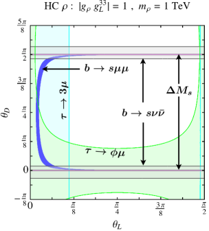
Figure 1: Allowed regions in the $(\theta_{L},\theta_{D})$ plane in the HC $\rho$ model for $m_{\rho}=1\,\text{TeV}$ and $g_{\rho}\,g_{L}^{33}=1$. The $b\to s\mu^{+}\mu^{-}$ anomaly can be explained in the blue region while the constraints from $\Delta M_{s}$, $\mathcal{B}(\tau\to 3\mu)$, $\mathcal{B}(\tau\to\phi\mu)$, and $\mathcal{B}(B\to K^{(*)}\nu\bar{\nu})$ are satisfied in the magenta, cyan, green, and gray regions, respectively.

Now we investigate the parameter space of the model consistent with the flavor measurements. Theoretical input for our evaluation is summarized in Table 3. In Fig. 1, we show a plane view of allowed regions in the $(\theta_{L},\theta_{D})$ plane for $m_{\rho}=1\,\text{TeV}$ and $g_{\rho}\,g_{L}^{33}=1$ constrained from each observable: the $b\to s\ell^{+}\ell^{-}$ global fit in blue [Eq.(4.18)], $\Delta M_{s}$ in magenta [Eq.(4.29)], $\mathcal{B}(\tau\to 3\mu)$ in cyan, $\mathcal{B}(\tau\to\phi\mu)$ in green [Eq.(4.23)], and $\mathcal{B}(B\to K^{(*)}\nu\bar{\nu})$ in gray [Eq.(4.20)], as denoted in the figure. Note that $\Delta M_{s}$ is precisely measured at experiments and thus new physics contributions are allowed only within the theoretical uncertainties in Table 3. One easily sees that the constraint from the $B_{s}$ mixing (magenta region) is much stringent $|\theta_{D}|\ll 1$, while the other constraints are consistent with the $b\to s\mu^{+}\mu^{-}$ anomaly (blue region) in some limited regions.

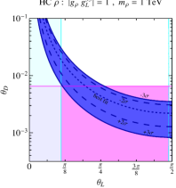
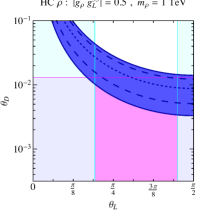
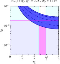
Figure 2: Allowed regions of the flavor constraints for various choice of $|g_{\rho}\,g_{L}^{33}|$ with $m_{\rho}=1\,\text{TeV}$ near $\theta_{D}\sim 0$. The significant constraints from $\Delta M_{s}$ (magenta), $\mathcal{B}(\tau\to 3\mu)$ (cyan), and the $b\to s\mu^{+}\mu^{-}$ global fit (blue) are shown whereas the others are simply omitted. The best-fit point, $\pm 2\sigma$, and $\pm 3\sigma$ ranges to explain the $b\to s\mu^{+}\mu^{-}$ anomaly are presented with dotted, dashed, and solid curves, respectively.

To more precisely see the allowed region near $\theta_{D}\sim 0$, in Fig. 2 we show the close-up version focused on the $\theta_{D}\sim 0$ region, for various values of $g_{\rho}g_{L}^{33}$ with $m_{\rho}=1\,\text{TeV}$ fixed, where we have taken the significant constraints, namely from $\Delta M_{s}$, $\mathcal{B}(\tau\to 3\mu)$, and the $b\to s\mu^{+}\mu^{-}$ global fit. In the close-up plot, we have taken the parameter range favored up to $\pm 3\sigma$ level for the $b\to s\mu^{+}\mu^{-}$ anomaly. For $|g_{\rho}\,g_{L}^{33}|\gtrsim 1$, it turns out that the $b\to s\mu^{+}\mu^{-}$ anomaly is not consistent with the constraints from $\Delta M_{s}$ and $\mathcal{B}(\tau\to 3\mu)$ in the present model. As for the range $0.35\lesssim|g_{\rho}\,g_{L}^{33}|\lesssim 1$, several comments are in order:

• We found that there are two isolated regions, $\theta_{L}\lesssim\pi/4$ (“left-side”) and $\theta_{L}\sim\pi/2$ (“right-side”), where all the constraints are (marginally) satisfied.

• The left-side spot is barely viable when the $b\to s\mu^{+}\mu^{-}$ anomaly is $3\sigma$ above in terms of the coefficient $C_{9}^{\mu\mu}$ from the best-fit point ($C_{9}^{\mu\mu}|_{\rm best}=-0.61$ Capdevila:2017bsm ), where $C_{9}^{\mu\mu}|_{+3\sigma}=-0.23$, which means that the deviation from the SM has to be rather small.

• On the other hand, the right-side spot fairly satisfies all the constraints. In particular, the point of $\theta_{L}=\pi/2$ can accommodate the best fit point for the $b\to s\mu^{+}\mu^{-}$ anomaly. Note that $\theta_{L}=\pi/2$ is the point in which $\tau$ in the gauge basis is exactly equivalent to $\mu$ in the mass basis. In this case, the lepton sector only has the connection to the HC $\rho$ from the $\mu$-$\mu$-$\rho$ term.

For $|g_{\rho}\,g_{L}^{33}|\lesssim 0.35$ we also found that the two allowed spots (which were divided by the $\tau\to 3\mu$ constraint) are merged into a single spot and then the region near $\theta_{L}\sim\pi/2$ is only allowed. In Fig. 3, we survey the allowed range of $|g_{\rho}\,g_{L}^{33}|$ for the case $\theta_{L}=\pi/2$. The result implies that the present model for $\theta_{L}=\pi/2$ requires $|g_{\rho}\,g_{L}^{33}|\gtrsim 0.1$ in order to explain the $b\to s\mu^{+}\mu^{-}$ anomaly consistently with the bound from $\Delta M_{s}$.

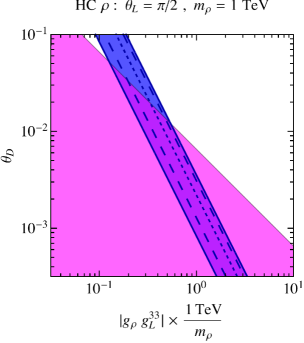
Figure 3: The allowed range in terms of $|g_{\rho}\,g_{L}^{33}|$ and $\theta_{D}$ for the fixed value $\theta_{L}=\pi/2$ (“right-side” spot). Conventions of the plots are the same as in Fig. 2.

To summarize, we investigated the allowed regions in the parameter space of $\theta_{L}$, $\theta_{D}$, and $|g_{\rho}\,g_{L}^{33}|$, which satisfy all the flavor constraints. The situation is then divided by two cases; $\theta_{L}\lesssim\pi/4$ (“left-side”) and $\theta_{L}\sim\pi/2$ (“right-side”). As a result, the allowed region exists in

$$~{}~{}0.35\lesssim\left|g_{\rho}\,g_{L}^{33}\right|\times\left(\frac{1\,\text{TeV}}{m_{\rho}}\right)\lesssim 1 \quad\text{(for left-side spot)}\,,$$ (4.33)

$$~{}~{}~{}\,0.1\lesssim\left|g_{\rho}\,g_{L}^{33}\right|\times\left(\frac{1\,\text{TeV}}{m_{\rho}}\right) \quad\text{(for right-side spot)}\,.$$ (4.34)

The left-side spot is considered as the $\tau$-dominant case where the $\tau$-$\tau$-$\rho$ coupling is relatively larger than the other lepton couplings to HC $\rho$ (including LFV.) On the other hand, the right-side spot only involves the $\mu$-$\mu$-$\rho$ coupling. Indeed, we have to pay attention to this difference when we consider collider limit at LHC as will be discussed in the next section.

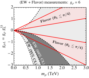
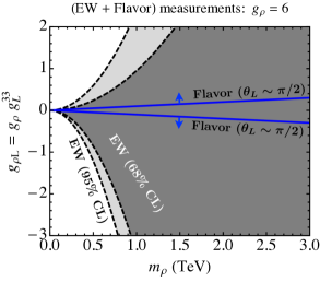
Figure 4: Summary plot for constraints from the EW precision measurements and from the flavor observables on the $(g_{\rho}g_{L}^{33},m_{\rho})$ plane fixing $g_{\rho}=6$ for $\theta_{L}\lesssim\pi/4$ (left) and $\theta_{L}\sim\pi/2$ (right). The (darker) gray region is allowed by the EW precision measurements at $95\%$ ($68\%$) C.L. The regions in red (blue) line boundaries are favored by the $b\to s\mu^{+}\mu^{-}$ data that satisfies all the other flavor constraints, for $\theta_{L}\lesssim\pi/4$ ($\theta_{L}\sim\pi/2$).

The combined plots with the constraint from the EW precision measurements are shown in Fig. 4 on the $(g_{\rho}g_{L}^{33},\,m_{\rho})$ plane for the $\theta_{L}\lesssim\pi/4$ and $\theta_{L}\sim\pi/2$ cases. The regions in red (blue) line boundaries are favored by the $b\to s\mu^{+}\mu^{-}$ data, along with the other constraints, for the left-side ($\theta_{L}\lesssim\pi/4$) and right-side ($\theta_{L}\sim\pi/2$) spots. The shaded regions show $68\%$ and $95\%$ C.L. constraints from the EW measurements as obtained in Sec. 3.5. (Note that, for the $\theta_{L}\sim\pi/2$ case, the EW limit is obtained by combining the $R_{b}$ and $A_{\rm FB}^{(0,\mu)}$ constraints.) In the figure, the reference number $g_{\rho}=6$ is taken. We can see that the favored regions from the $b\to s\mu^{+}\mu^{-}$ data are consistent with the $95\%$ C.L. EW precision measurements. One also finds that, in the $1\sigma$ range ($68\%$ C.L.), the EW precision measurements exclude the HC rho mass $m_{\rho}\gtrsim 1.8\,\text{TeV}$ and the positive value of $g_{\rho}\,g_{L}^{33}$ for the left-side spot case with $\theta_{L}\lesssim\pi/4$. The allowed parameter space can be examined by direct searches at the LHC. It will be discussed below.

5 Collider-related issues

In this section, we discuss constraints from the latest null results in the new physics searches and future prospects at the $13\,\text{TeV}$ LHC. The HC $\rho$’s as well as the HC $\pi$’s will be resonantly, or non-resonantly produced at the hadron collision machinery, to be constrained by the present experimental data.

5.1 Typical constraints on HC $\pi$

Even though the details of the HC pion sector is out of our major interests, we briefly comment on possible constraints on this part. Here, we focus on the color-singlet isospin-singlet HC pion $\pi^{0}_{(1)^{\prime}}$ as a typical signature. Two types of interactions can be derived for the $\pi_{(1)^{\prime}}^{0}$. The first one is from the global chiral anomalies of hypercolor fermions, which are represented by the covariantized WZW terms in the present non-Abelian $SU(8)_{F_{L}}\times SU(8)_{F_{R}}$ case Jia:2012kd ; Matsuzaki:2015che (based on the discussion on Ref. Kaymakcalan:1983qq ),

$$S_{\text{WZW}} \ni-\frac{N_{\rm HC}}{48\pi^{2}}\int_{M^{4}}\Bigg{\{}{\rm tr}\left[(d{\cal L}{\cal L}+{\cal L}d{\cal L})\alpha+(d{\cal R}{\cal R}+{\cal R}d{\cal R})\beta\right]+i{\rm tr}\left[d{\cal L}dU{\cal R}U^{\dagger}-d{\cal R}dU^{\dagger}{\cal L}U\right]\Bigg{\}}$$

$$=-\frac{N_{\rm HC}}{12\pi^{2}f_{\pi}}\int_{M^{4}}{\rm tr}\left[(3d{\cal V}d{\cal V}+d{\cal A}d{\cal A})\pi+{\cal O}(\pi^{2})\right],$$ (5.1)

where we focus on ${\cal V}$-${\cal V}$-$\pi$ interactions. $M^{4}$ means the four-dimensional Minkowski manifold, $U$ denotes the chiral nonlinear basis $U\equiv e^{2i\pi/f_{\pi}}=\xi_{L}^{\dagger}\xi_{R}$, and the differential one-forms are defined as

$$\alpha=-idUU^{\dagger},\quad\beta=-iU^{\dagger}dU.$$ (5.2)

One-form of the external vector gauge boson includes the gluon as

$${\cal V}=\frac{{\cal R+L}}{2}\ni g_{s}G^{a}(\sqrt{2}T_{(8)a}).$$ (5.3)

Then we encounter the trace, ${\rm tr}\left[(\sqrt{2})^{2}T_{(8)a}T_{(8)b}T_{(1)^{\prime}}\right]=\delta^{ab}/4\sqrt{3}$, which leads to

$$S_{\text{WZW}}(\pi^{0}_{(1)^{\prime}}GG) =-\frac{N_{\rm HC}}{16\sqrt{3}\pi^{2}}\frac{g_{s}^{2}}{f_{\pi}}\int_{M^{4}}\pi^{0}_{(1)^{\prime}}\,dG^{a}dG^{a}$$

$$=-\frac{N_{\rm HC}}{16\sqrt{3}\pi^{2}}\frac{g_{s}^{2}}{f_{\pi}}\frac{1}{4}\int_{M^{4}}\!\!\!\!\!d^{4}x\ \pi^{0}_{(1)^{\prime}}\,G_{\mu\nu}^{a}G_{\rho\sigma}^{a}\varepsilon^{\mu\nu\rho\sigma},$$ (5.4)

where we used the relation $dG^{a}dG^{a}=d^{4}x\,G_{\mu\nu}^{a}G_{\rho\sigma}^{a}\varepsilon^{\mu\nu\rho\sigma}/4$. This effective action describes the anomaly-induced $G$-$G$-$\pi^{0}_{(1)^{\prime}}$ interaction. (Note that $G$ indicates gluon in this article.)

Another possible origin of the $G$-$G$-$\pi^{0}_{(1)^{\prime}}$ coupling comes from a top-quark loop contribution constructed from the $t$-$\bar{t}$-$\pi^{0}_{(1)^{\prime}}$ interaction, which could be, in the present model, induced through an extended HC as given in Eq.(2.60). As discussed in Ref. Kauffman:1993nv the amplitude corresponding to such a top-loop contribution is generically written down

$${\cal M}\left(\pi^{0}_{(1)^{\prime}}\to G^{a}(p_{1\mu})G^{b}(p_{2\nu})\right)=-ig_{A}r_{y}\,\delta^{ab}\varepsilon^{\mu\nu\rho\sigma}p_{1\rho}p_{2\sigma}\tau f(\tau)\epsilon^{\ast}_{\mu}\epsilon^{\ast}_{\nu},$$ (5.5)

with the factor $g_{A}=\alpha_{s}/(2\pi v_{\rm VEV})$, the $t$-$\bar{t}$-$\pi^{0}_{(1)^{\prime}}$ coupling strength $r_{y}$ being real and defined as a ratio to the SM like top-Higgs case ($m_{t}\gamma_{5}/v_{\rm VEV}$), and the gluon polarization vectors $\epsilon_{\mu,\nu}$. Here, we adopt the Feynman rule of the fundamental pseudoscalar to parametrize the coupling. The loop function $f(\tau)$ is a function of the parameter $\tau\equiv 4m_{t}^{2}/M_{\pi^{0}_{(1)^{\prime}}}^{2}$ as

$$f(\tau)=\begin{cases}\displaystyle\left[\sin^{-1}\left(\sqrt{\frac{1}{\tau}}\right)\right]^{2}&\text{for }\tau\geq 1,\\ \displaystyle-\frac{1}{4}\left[\ln\left(\frac{\eta_{+}}{\eta_{-}}\right)-i\,\pi\right]^{2}&\text{for }\tau<1,\end{cases}$$ (5.6)

with $\eta_{\pm}=1\pm\sqrt{1-\tau}$.

Combined with the above two sources, the squared amplitudes are computed as

$$\left|\overline{{\cal M}}\right|^{2}_{\rm WZW} =1024A^{2}(p_{1}\cdot p_{2})^{2},$$ (5.7)

$$\left|\overline{{\cal M}}\right|^{2}_{\rm top} =16\,g_{A}^{2}|r_{y}\tau f(\tau)|^{2}(p_{1}\cdot p_{2})^{2},$$ (5.8)

$$\left|\overline{{\cal M}}\right|^{2}_{\rm int} =128Ag_{A}\left[r_{y}\tau f(\tau)+\left(r_{y}\tau f(\tau)\right)^{\ast}\right](p_{1}\cdot p_{2})^{2},$$ (5.9)

$${\left|\overline{{\cal M}}\right|^{2}} ={\left|\overline{{\cal M}}\right|^{2}_{\rm WZW}+\left|\overline{{\cal M}}\right|^{2}_{\rm top}+\left|\overline{{\cal M}}\right|^{2}_{\rm int},}$$ (5.10)

with the factor

$$A=-\frac{N_{\rm HC}}{16\sqrt{3}\pi^{2}\cdot 4}\frac{g_{s}^{2}}{f_{\pi}}.$$ (5.11)

Through the relations $2\,p_{1}\cdot p_{2}=M_{\pi^{0}_{(1)^{\prime}}}^{2}$ and $\Gamma({\pi^{0}_{(1)^{\prime}}}\to GG)=|\overline{{\cal M}}|^{2}/(2\times 16\pi M_{\pi^{0}_{(1)^{\prime}}})$, we obtain

$$\Gamma({\pi^{0}_{(1)^{\prime}}}\to GG) =\frac{\left(M_{\pi^{0}_{(1)^{\prime}}}\right)^{3}}{\pi}\left\{8A^{2}+\frac{1}{8}g_{A}^{2}|r_{y}\tau f(\tau)|^{2}+Ag_{A}{r_{y}\left[\tau f(\tau)+\left(\tau f(\tau)\right)^{\ast}\right]}\right\}$$

$$=\frac{\left(M_{\pi^{0}_{(1)^{\prime}}}\right)^{3}}{\pi}\left\{8A^{2}+\frac{1}{8}g_{A}^{2}|r_{y}\tau f(\tau)|^{2}+{2Ag_{A}r_{y}\text{Re}\left[\tau f(\tau)\right]}\right\}.$$ (5.12)

Through the well known formula for cross section with a spin-$J$ resonance that arises from a proton-proton collision with gluonic initial state Franceschini:2015kwy

$$\sigma(GG\to\pi_{(1)^{\prime}}^{0}\to\gamma\gamma)=\frac{2J+1}{s}C_{GG}\frac{\Gamma(\pi_{(1)^{\prime}}^{0}\to GG)}{M_{\pi_{(1)^{\prime}}^{0}}}\frac{\Gamma({\pi_{(1)^{\prime}}^{0}}\to\gamma\gamma)}{\Gamma_{{\pi_{(1)^{\prime}}^{0}}}},$$ (5.13)

(where $s$ is the center of mass energy and $C_{GG}|_{13\,\text{TeV}}=2137$ Franceschini:2015kwy denotes the luminosity coefficient for a pair of gluons as initial partons,) we can immediately calculate the diphoton cross section.

First, we shall consider the simplest case with $r_{y}=0$, (namely, no coupling to top quark pair.) In this case, we estimate the diphoton cross section

$${\sigma(GG\to\pi_{(1)^{\prime}}^{0}\to\gamma\gamma)\Bigg{|}_{r_{y}=0}}\sim{0.1\,\text{fb}}\times\left[\frac{N_{\rm HC}}{3}\right]^{2}\left[\frac{\alpha_{s}}{0.1}\right]^{2}\left[\frac{{\mathcal{B}}(\pi_{(1)^{\prime}}^{0}\to\gamma\gamma)}{{10^{-3}}}\right]\left(\frac{M_{\pi_{(1)^{\prime}}^{0}}}{f_{\pi}}\right)^{2}.$$ (5.14)

Note that, in the case of $r_{y}=0$, $\mathcal{B}(\pi_{(1)^{\prime}}^{0}\to\gamma\gamma)$ is completely free from the $\pi_{(1)^{\prime}}^{0}$ mass dependence because $\pi_{(1)^{\prime}}$ decays only to the massless final states, $2\gamma$ and $2G$. Hence the diphoton cross section in Eq.(5.14) is controlled only by the ratio $(M_{\pi_{(1)^{\prime}}^{0}}/f_{\pi})$. To survey a generic parameter space in the present model, we shall momentarily take the value of $M_{\pi_{(1)^{\prime}}^{0}}$ in a range from ${\cal O}(100)$ GeV [low mass] up to ${\cal O}({\rm TeV})$ [high mass] , and discuss the phenomenological constraints from the diphoton cross section of Eq.(5.14).

In the high mass case ($M_{\pi_{(1)^{\prime}}^{0}}\sim\text{TeV}$), the estimated diphoton cross section in Eq.(5.14) is compared with the $95\%$ C.L. upper bound on fiducial cross sections as $\sigma_{\rm ggF}^{\rm spin\,0}(\gamma\gamma)\equiv\sigma(GG\to[\text{spin-0 resonance}]\to\gamma\gamma)\lesssim 1\,\text{fb}$ for narrow-width resonance with mass $\sim 1\,\text{TeV}$ reported in Refs. ATLAS:2016eeo ; Khachatryan:2016yec . Thus we can naively say that the prediction in the HC theory has a tight tension with the present experimental data unless $M_{\pi_{(1)^{\prime}}^{0}}/f_{\pi}\lesssim 3$. To be consistent with the above bound for $M_{\pi_{(1)^{\prime}}^{0}}\sim 1\,\text{TeV}$ implies that the HC pion decay constant $f_{\pi}$ should be (at least) as large as around $v_{\rm VEV}$. However, several nonperturbative estimates with some approximation Harada:2003dc ; Kurachi:2006ej , as well as recent lattice simulations in QCD with many flavors Appelquist:2014zsa ; Aoki:2016wnc , suggest the mass relation in magnitude of $m_{\rho}\sim{\cal O}(10)f_{\pi}$ (for the $m_{\rho}/f_{\pi}$ ratio in QCD with 8 flavors, see also Ref. Matsuzaki:2015sya .) Therefore, the diphoton constraint ($M_{\pi_{(1)^{\prime}}^{0}}/f_{\pi}\lesssim 3$) along with the estimated mass relation ($m_{\rho}\sim{\cal O}(10)f_{\pi}$) indicates the bound on the HC rho mass scale as $m_{\rho}\gtrsim 3\,\text{TeV}$.

As for the low mass case, the ATLAS $8\,\text{TeV}$ bound is available in the range $65$ – $200\,\text{GeV}$. In particular, the fluctuating $95\%$ C.L. bounds around $65$ – $100\,\text{GeV}$ is $\sim 50\,\text{fb}$ as a crude average Aad:2014ioa , which corresponds to $\sim 250\,\text{fb}$ at $13\,\text{TeV}$ Franceschini:2015kwy . Thereby the diphoton bound looks not serious for $M_{\pi_{(1)^{\prime}}^{0}}\lesssim 200\,\text{GeV}$.

For an intermediate-mass case ($200\,{\rm GeV}\lesssim M_{\pi_{(1)^{\prime}}^{0}}\lesssim 1\,\text{TeV}$) – referred to as the EW-mass case hereafter – the (fluctuating) $13\,\text{TeV}$ $95\%$ C.L. upper bound for $\sigma_{\rm ggF}^{\rm spin\,0}(\gamma\gamma)$ is around $\sim 1\,\text{fb}$ in the range $500\,\text{GeV}$ – $1\,\text{TeV}$ ATLAS:2016eeo ; Khachatryan:2016yec . Below $500\,\text{GeV}$, the exclusion limit gets reduced such as $\sigma_{\rm ggF}^{\rm spin\,0}(\gamma\gamma)\sim 10\,\text{fb}$ for $M_{\pi_{(1)^{\prime}}^{0}}=200\,\text{GeV}$ ATLAS:2016eeo ; $\sim 4\,\text{fb}$ for $M_{\pi_{(1)^{\prime}}^{0}}=300\,\text{GeV}$; and $\sim 2\,\text{fb}$ for $M_{\pi_{(1)^{\prime}}^{0}}=400\,\text{GeV}$, (here we do not take care of the rapid fluctuations in the cross section curves depicting $95\%$ C.L. upper bounds.) Those diphoton limits can safely be evaded if the decay constant $f_{\pi}$ is set to be as large as, e.g., $\sim 500\,\text{GeV}$ and the HC rho mass scale is $m_{\rho}\gtrsim 5\,\text{TeV}$, which is consistent with the aforementioned relation, $m_{\rho}\sim{\cal O}(10)\,f_{\pi}\sim{\cal O}(10)\,M_{\pi_{(1)^{\prime}}^{0}}$, based on the nonperturbative observation.

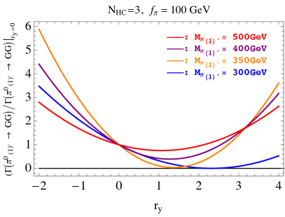
Figure 5: Curves that show the ratio $\Gamma(\pi_{(1)^{\prime}}^{0}\to GG)/\Gamma(\pi_{(1)^{\prime}}^{0}\to GG)|_{r_{y}=0}$ under the four different choices of $M_{\pi_{(1)^{\prime}}^{0}}$ in $f_{\pi}=10^{2}\,\text{GeV}$ and $N_{\rm HC}=3$.

The condition $M_{\pi_{(1)^{\prime}}^{0}}/f_{\pi}\lesssim 3$ is violated, for example, if $f_{\pi}\sim 100\,\text{GeV}$ and $M_{\pi_{(1)^{\prime}}^{0}}\gtrsim 300\,\text{GeV}$. In such a case, we may still evade the $95\%$ C.L. upper bound at $13\,\text{TeV}$ by taking the additional contribution from the coupling to top quark (i.e. $r_{y}\neq 0$) to make the partial width $\Gamma(\pi_{(1)^{\prime}}^{0}\to GG)$ reduced. Such a reduction can originate from the interference effect in Eq.(5.12). We illustrate this case in the following. In Fig. 5, we show how $\Gamma(\pi_{(1)^{\prime}}^{0}\to GG)$ is changed under the presence of nonzero $r_{y}$ in $f_{\pi}=10^{2}\,\text{GeV}$ and $N_{\rm HC}=3$ . For $M_{\pi_{(1)^{\prime}}^{0}}=300-350\,\text{GeV}$, a suitably tuned $r_{y}$ leads to an (almost) vanishing value of $\Gamma(\pi_{(1)^{\prime}}^{0}\to GG)$, while for $M_{\pi_{(1)^{\prime}}^{0}}\gtrsim 400\,\text{GeV}$, only $\lesssim 50\%$ cancellation is possible at most, which may be enough to alleviate the tension for $M_{\pi_{(1)^{\prime}}^{0}}\sim 400\,\text{GeV}$. Let us remind that the constraint on the cross section for $M_{\pi_{(1)^{\prime}}^{0}}=300\,\text{GeV}$ ($\sigma_{\rm ggF}^{\rm spin\,0}(\gamma\gamma)\lesssim 4\,\text{fb}$) is looser than that for $M_{\pi_{(1)^{\prime}}^{0}}=400\,\text{GeV}$ ($\sigma_{\rm ggF}^{\rm spin\,0}(\gamma\gamma)\lesssim 2\,\text{fb}$). Thus, the interference contribution helps us to revive the possibility of $\pi_{(1)^{\prime}}^{0}$ with the mass around $400\,\text{GeV}$ even when $f_{\pi}\sim 100\,\text{GeV}$, while no cancellation may be required for $300\,\text{GeV}\lesssim M_{\pi_{(1)^{\prime}}^{0}}\lesssim 400\,\text{GeV}$. This consequence is followed by discussion for a LHC bound on the HC $\rho$ meson mass.

Another constraint comes from the scalar leptoquark search derived from a non-resonant pair production of $\pi_{(3)}^{0}$ in our model, as has been reported by ATLAS in Ref. Aaboud:2016qeg for first and second generation leptoquarks. The result says that the corresponding mass scale of $\pi_{(3)}^{0}$ should be $\gtrsim 1050-1100\,\text{GeV}$ at $95\%$ C.L. assuming $100\%$ branching fraction for a $\pi_{(3)}^{0}$ decay. We note that final states are less ambiguous since possible decay branches are limited, but still there is a parameter dependence on $a$ in general as shown in Eq.(2.76). Here, we provide a simple conclusion such that the bound from the pair production is harmless if a typical mass scale of HC pions is sufficiently greater than $1\,\text{TeV}$. As shown in Eq.(2.41), vector leptoquarks indeed obtain $\sim 3\,\text{TeV}$ masses for $\Lambda_{\rm HC}\sim 1\,\text{TeV}$, which come most dominantly through QCD gluon exchange corrections amplified due to the characteristic feature of many flavor QCD. Thus our heavy HC pion scenario can still avoid the current scalar leptoquark bound.

5.2 Resonant productions of HC $\rho$

In this part, we discuss constraints from resonance searches at the $13\,\text{TeV}$ LHC, which provide stringent bounds on mass scales of HC rho mesons directly.

5.2.1 Basic backgrounds

As we have pointed out, although the $V_{\rm SM}$-$\rho$ mixing (in the covariantized HLS formulation of this model) generates mass splittings among HC $\rho$ mesons in physical eigenstates, only a few-percent splittings are allowed because of the large coupling $g_{\rho}\sim 6$ as in Eq.(2.79), which would be supported from the QCD-like vector dominance. Thereby, it is a good approximation to consider all of the HC $\rho$ components to be degenerated in the common mass scale $m_{\rho}$, and interactions induced through such mass mixings to be negligible.

We should also recall that the mixing angles $\theta_{D}$ and $\theta_{L}$ defined in Eq.(4.2) were already restricted from the EW (in Sec. 3.5) and flavor (in Sec. 4) observables. To address the $b\to s\mu^{+}\mu^{-}$ anomaly consistently with the other constraints, we found that $\theta_{D}$ needs to be much tiny such as $\theta_{D}\sim 10^{-2}$ – $10^{-3}$. Thus we can take the limit of $\theta_{D}\to 0$ for all the calculations on collider phenomena (though the minuscule values are mandatory for addressing the $b\to s\mu^{+}\mu^{-}$ anomaly.) On the other hand, it has turned out that the favored regions for $\theta_{L}$ are categorized by two spots, $\theta_{L}\lesssim\pi/4$ and $\theta_{L}\sim\pi/2$ depending on the magnitude of the coupling $g_{\rho L}\equiv g_{\rho}g_{L}^{33}$. This angle $\theta_{L}$ determines the relative coupling strength of HC $\rho$ mesons to $2\tau$ and $2\mu$, which are $\cos^{2}{\theta_{L}}$ and $\sin^{2}{\theta_{L}}$, respectively, hence the coupling to $2\tau$ becomes dominant for $\theta_{L}\lesssim\pi/4$, while the coupling to $2\mu$ does for $\theta_{L}\sim\pi/2$. Thus, significant collider bounds would be derived from the $2\tau$ and $2\mu$ channel searches, depending on the $\theta_{L}$. To be concrete and conservative, we shall hereafter take $\theta_{L}=0$ (for the $2\tau$ channel) and $\theta_{L}=\pi/2$ (for the $2\mu$ channel) as the reference values corresponding to the two cases.

To calculate resonant processes, values of total decay widths are important. Possible decay branches are shared by a pair of the SM fermions and a pair of HC pions [see Appendix A]. Here, we assume that the latter case is kinematically blocked ($m_{\rho}<2m_{\pi}$), which turns out to be reasonable. To see how it works, first recall that some HC pion masses should be sufficiently as heavy as ${\cal O}(1)\,\text{TeV}$, as listed in Eq.(2.41). More precisely, we see from Eq.(2.41) that when $f_{\pi}\sim{\cal O}(100)\,\text{GeV}$ and $\Lambda_{\rm HC}\sim 1\,\text{TeV}$, the mass of the color-singlet isospin-triplet mesons is $\sim 2\,\text{TeV}$, while those of the colored mesons are $\sim 3\,\text{TeV}$ ($\sim 4\,\text{TeV}$) for color triplets (color octets). To make sure how the decay channels to HC pion pairs open, we list up the total values of the final-state particle masses ($m_{\pi\pi}$): (c.f., Appendix A),

• $\rho^{0}_{(3)}\to\bar{\pi}^{0}_{(3)}\pi^{0}_{(1)^{\prime}}$ : $m_{\pi\pi}\sim(3+{\cal O}(0.1))\,\text{TeV}$,

• $\rho^{\alpha}_{(3)}\to\bar{\pi}^{\alpha}_{(3)}\pi^{0}_{(1)^{\prime}}$ : $m_{\pi\pi}\sim(3+{\cal O}(0.1))\,\text{TeV}$,

• $\rho^{0}_{(8)}\to\bar{\pi}^{0}_{(3)}\pi^{0}_{(3)}$ : $m_{\pi\pi}\sim(3+3)\,\text{TeV}=6\,\text{TeV}$,

• $\rho^{\alpha}_{(8)}\to\bar{\pi}^{0}_{(3)}\pi^{\alpha}_{(3)}$ : $m_{\pi\pi}\sim(3+3)\,\text{TeV}=6\,\text{TeV}$,

• $\rho^{0}_{(1)^{\prime}}\to\bar{\pi}^{0}_{(3)}\pi^{0}_{(3)}$ : $m_{\pi\pi}\sim(3+3)\,\text{TeV}=6\,\text{TeV}$,

• $\rho^{\alpha}_{(1)^{\prime}}\to\bar{\pi}^{\beta}_{(1)}\pi^{\gamma}_{(1)^{\prime}}$ : $m_{\pi\pi}\sim(1+2)\,\text{TeV}=3\,\text{TeV}$,

• $\rho^{\alpha}_{(1)}\to\bar{\pi}^{\beta}_{(1)}\pi^{\gamma}_{(1)}$ : $m_{\pi\pi}\sim(1+{2})\,\text{TeV}={3}\,\text{TeV}$.

Then, additional contributions to the HC rho’s decay branches appear when $m_{\rho}\gtrsim 3\,\text{TeV}$ at the present benchmark point, $f_{\pi}\sim{\cal O}(100)\,\text{GeV}$ and $\Lambda_{\rm HC}\sim 1\,\text{TeV}$. On the other hand, when $f_{\pi}$ is somewhat greater than $\sim 100\,\text{GeV}$ (with a sizable explicit breaking scale $m^{0}_{F}$), the HC pions becomes heavier and we may block the HC rho’s decays to the HC pions consistently, keeping the relation $m_{\rho}\sim{\cal O}(10)f_{\pi}$ intact.

Thus our assumption $m_{\rho}<2m_{\pi}$ may be justified even in the range $m_{\rho}\gtrsim 3\,\text{TeV}$, so that we may be able to ignore decays to HC pion pairs. Of interest enough is then that all of the physical HC $\rho$ components have the common value in the total width as

$$\Gamma_{\rho}=\frac{g_{\rho L}^{2}m_{\rho}}{48\pi},$$ (5.15)

where we simply ignored tiny contributions through mixing effects. Details of partial widths are provided in appendix C. The curve of the ratio $\Gamma_{\rho}/m_{\rho}$ as a function of $g_{\rho L}$ is illustrated in Fig. 6.

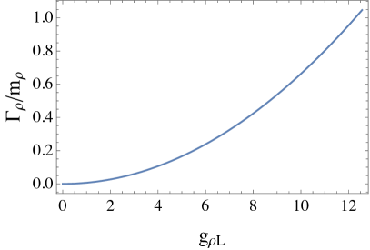
Figure 6: The ratio $\Gamma_{\rho}/m_{\rho}$ in Eq.(5.15) as a function of $g_{\rho L}$.

5.2.2 Forms of resonant cross sections

We summarize the forms of differential production (on the solid angle $\Omega$ in the center-of-mass flame) cross section at the LHC. As we pointed out, we set the mixing angles $\theta_{D}=0$ and $\theta_{L}=0$ or $\pi/2$ and consider that all of the HC $\rho$ mesons are completely degenerated. We note that in the limit of $\theta_{D}=0$, the possible initial state is $b\bar{b}$ only. Due to this mass degeneracy, we should take all of the HC $\rho$ contributions simultaneously.

First, we look at the dijet final state that originates from $b$ (or anti-$b$) quark where $\rho_{(8)}^{0}$, $\rho_{(8)}^{3}$, $\rho_{(1)}^{3}$, $\rho_{(1)^{\prime}}^{3}$, and $\rho_{(1)^{\prime}}^{0}$ contribute as intermediate states ($b\bar{b}\to\text{$\rho$'s}\to b\bar{b}$). The differential cross section forms for color-singlets and color-octets are summarized as

$$\left(\frac{d\sigma_{jj}}{d\Omega}\right)_{\text{singlet}} =\frac{1}{2\widehat{s}}\frac{1}{32\pi^{2}}\frac{1}{2^{2}}\frac{1}{3^{2}}\frac{4\,g_{\rho L}^{4}f^{bb}_{\rm singlet}}{(\widehat{s}-m_{\rho}^{2})^{2}+(m_{\rho}\Gamma_{\rho})^{2}}\left(\frac{\widehat{s}}{2}(1+\cos{\theta})\right)^{2},$$ (5.16)

$$\left(\frac{d\sigma_{jj}}{d\Omega}\right)_{\text{octet}} =\frac{1}{2\widehat{s}}\frac{1}{32\pi^{2}}\frac{1}{2^{2}}\frac{1}{3^{2}}\frac{4\,g_{\rho L}^{4}f^{bb}_{\rm octet}}{(\widehat{s}-m_{\rho}^{2})^{2}+(m_{\rho}\Gamma_{\rho})^{2}}\left(\frac{\widehat{s}}{2}(1+\cos{\theta})\right)^{2},$$ (5.17)

where we take all of the quarks are massless. Now, both of color-octets and color-singlets contribute in $s$-channels, and no interference term appears between the singlet amplitudes and those of octets. Here, the following relations hold in the hatted Mandelstam variables in the parton system

$$\widehat{s}+\widehat{t}+\widehat{u}\simeq 0,\quad\widehat{t}\simeq-\frac{\widehat{s}(1-\cos{\theta})}{2},\quad\widehat{u}\simeq-\frac{\widehat{s}(1+\cos{\theta})}{2},$$ (5.18)

where the angle $\theta$ is defined in the center-of-mass frame. The factors $f^{bb}_{\rm singlet}$ and $f^{bb}_{\rm octet}$ represent summations of all possible combinations of the couplings plus the overall color factor,

$$f^{bb}_{\rm singlet} ={3^{2}}\times\left[\left(-\frac{1}{4}\right)^{2}+\left(-\frac{1}{4\sqrt{3}}\right)^{2}+\left(\frac{1}{4\sqrt{3}}\right)^{2}\right]^{2}\simeq 0.098,$$ (5.19)

$$f^{bb}_{\rm octet} ={2}\times\left[\left(-\frac{1}{\sqrt{2}}\right)^{2}+\left(\frac{1}{\sqrt{2}}\right)^{2}\right]^{2}=2.$$ (5.20)

Next, we go for the ditau and dimuon final states, where $\rho_{(3)}^{3}$, $\rho_{(3)}^{0}$, $\rho_{(1)}^{3}$, $\rho_{(1)^{\prime}}^{3}$, $\rho_{(1)^{\prime}}^{0}$ are possible intermediate states ($b\bar{b}\to\text{$\rho$'s}\to\tau\bar{\tau}/\mu\bar{\mu}$). We note that in the present limit ($\theta_{D}=0$ and $\theta_{L}=0$ or $\pi/2$), the cross section formula for the ditau channel is exactly the same as that for the dimuon channel. In the present case, color-triplets/-singlets contribute in $t$/$s$-channels, and interference terms are observed between the color-triplets and color-singlets. The differential cross section forms for color-singlets, color-triplets, and interferences are summarized as

$$\left(\frac{d\sigma_{{\tau\tau/\mu\mu}}}{d\Omega}\right)_{\text{singlet}} =\frac{1}{2\widehat{s}}\frac{1}{32\pi^{2}}\frac{1}{2^{2}}\frac{1}{3^{2}}\frac{4\,g_{\rho L}^{4}f^{{\tau\tau/\mu\mu}}_{\rm singlet}}{(\widehat{s}-m_{\rho}^{2})^{2}+(m_{\rho}\Gamma_{\rho})^{2}}\left(\frac{\widehat{s}}{2}(1+\cos{\theta})\right)^{2},$$ (5.21)

$$\left(\frac{d\sigma_{{\tau\tau/\mu\mu}}}{d\Omega}\right)_{\text{triplet}} =\frac{1}{2\widehat{s}}\frac{1}{32\pi^{2}}\frac{1}{2^{2}}\frac{1}{3^{2}}\frac{4\,g_{\rho L}^{4}f^{{\tau\tau/\mu\mu}}_{\rm triplet}}{(\widehat{t}-m_{\rho}^{2})^{2}+(m_{\rho}\Gamma_{\rho})^{2}}\left(\frac{\widehat{s}}{2}(1+\cos{\theta})\right)^{2},$$ (5.22)

$$\left(\frac{d\sigma_{{\tau\tau/\mu\mu}}}{d\Omega}\right)_{\text{int}} =\frac{1}{2\widehat{s}}\frac{1}{32\pi^{2}}\frac{1}{2^{2}}\frac{1}{3^{2}}\frac{g_{\rho L}^{4}f^{{\tau\tau/\mu\mu}}_{\rm int}\left[(\widehat{s}-m_{\rho}^{2})(\widehat{t}-m_{\rho}^{2})+(m_{\rho}\Gamma_{\rho})^{2}\right]\times{2}}{\left[(\widehat{s}-m_{\rho}^{2})(\widehat{t}-m_{\rho}^{2})+(m_{\rho}\Gamma_{\rho})^{2}\right]^{2}+\left[m_{\rho}\Gamma_{\rho}(\widehat{t}-\widehat{s})\right]^{2}}(-1)\left(\frac{\widehat{s}}{2}(1+\cos{\theta})\right)^{2},$$ (5.23)

with

$$f^{{\tau\tau/\mu\mu}}_{\rm singlet} ={3}\times\left[\left(-\frac{1}{4}\right)^{2}+\left(-\frac{1}{4\sqrt{3}}\right)\left(\frac{\sqrt{3}}{4}\right)+\left(\frac{1}{4\sqrt{3}}\right)\left(-\frac{\sqrt{3}}{4}\right)\right]^{2}\simeq 0.012,$$ (5.24)

$$f^{{\tau\tau/\mu\mu}}_{\rm triplet} =3\times\left[\left(-\frac{1}{2}\right)^{2}+\left(\frac{1}{2}\right)^{2}\right]^{2}=0.75,$$ (5.25)

$$f^{{\tau\tau/\mu\mu}}_{\rm int} =3\times\left[\left(-\frac{1}{4}\right)^{2}+\left(-\frac{1}{4\sqrt{3}}\right)\left(\frac{\sqrt{3}}{4}\right)+\left(\frac{1}{4\sqrt{3}}\right)\left(-\frac{\sqrt{3}}{4}\right)\right]\left[\left(-\frac{1}{2}\right)^{2}+\left(\frac{1}{2}\right)^{2}\right]\simeq-0.094.$$ (5.26)

5.2.3 Results

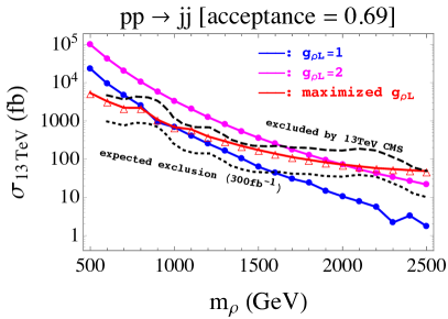
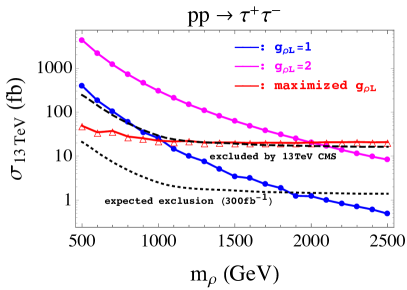
Figure 7: Naive constraints on $\sigma(pp\to jj)$ [left panel] and $\sigma(pp\to\tau\bar{\tau})$ [right panel] in $\theta_{D}=\theta_{L}=0$, where the CMS experimental results are from Refs. Sirunyan:2016iap ; Khachatryan:2016qkc . For the dijet resonance, we adopt the calculated value of acceptance ${\cal A}=0.69$ being different from the isotropic decays (${\cal A}\approx 0.6$) Sirunyan:2016iap . For the red curves showing ‘maximized $g_{\rho L}$’ being consistent with the requisites from flavor issues in Eq.(4.33), the value of $g_{\rho L}$ is tuned as $|g_{\rho L}|={1.0}\times(m_{\rho}/1\,\text{TeV})$. If $g_{\rho L}$ is greater than the tuned value (in each of $m_{\rho}$), we cannot address the flavor issues in the present model correctly. The regions above the black dashed (black dotted) lines are excluded (expected to be excluded after a $300\,\text{fb}^{-1}$ integrated luminosity accumulation) at $95\%$ C.L.s.

The convolution with the (anti-)bottom quark parton distribution function (PDF) inside the proton $f_{b/p}(x,\mu_{F})$ ($f_{\bar{b}/p}(x,\mu_{F})$) with the Bjorken $x$ and the PDF factorization scale $\mu_{F}$ is formulated as

$$\int_{\tau_{0}}^{1}dx_{1}\int_{\tau_{0}/x_{1}}^{1}dx_{2}\,\sigma\left[f_{b/p}(x_{1},\mu_{F})f_{\bar{b}/p}(x_{2},\mu_{F})+f_{b/p}(x_{2},\mu_{F})f_{\bar{b}/p}(x_{1},\mu_{F})\right].$$ (5.27)

Here, the total energy squared of the present LHC $s$($=13^{2}\,\text{TeV}^{2}$) is related to the total energy squared of the focused parton system $\widehat{s}$ as $\widehat{s}=x_{1}x_{2}s\equiv\tau\,s$. Kinematically, the minimal of the fraction $\tau$ is estimated as Han:2005mu

$$\tau_{0}={\frac{\{4m_{b}^{2},\ 4m_{\tau}^{2},\ 4m_{\mu}^{2}\}}{s}\sim\{4\times 10^{-7},\ 8\times 10^{-8},\ 3\times 10^{-10}\}},$$ (5.28)

where $\mu_{F}$ is set as $m_{\rho}$. We adopt the CTEQ6L1 PDF Pumplin:2002vw in calculations in Mathematica with the help of a PDF parser package, ManeParse_2.0 Clark:2016jgm , and set $\tau_{0}$ as $10^{-6}$ of the minimal value of the Bjorken $x$ in the CTEQ6L1 PDF set, which is not far from the values shown in Eq.(5.28).

In Fig. 7, we summarize the cross sections of $p(b)p(\bar{b})\to\text{$\rho$'s}\to j(b)j(\bar{b})$ (left panel) and $p(b)p(\bar{b})\to\text{$\rho$'s}\to\tau\bar{\tau}$ (right panel). To calculate the numerical integration including the PDF convolution in the Divonne method Friedman:1978ed ; Friedman:1981ak , we use the CUBA package Hahn:2004fe with the Mathlink protocol in Mathematica. The values of cross sections were cross-checked with MadGraph5_aMC@NLO Alwall:2011uj ; Alwall:2014hca , where the UFO-style model file Degrande:2011ua was generated by the FeynRules package Christensen:2008py ; Alloul:2013bka . For estimating the acceptance ${\cal A}$ of dijet events, we generated parton-level events in MadGraph5_aMC@NLO and analyzed them in the ROOT framework Brun:1997pa with the help of ExRootAnalysis, which is a part of the integrated package of MadGraph5_aMC@NLO. We obtained ${\cal A}\simeq 0.69$ in our case, which a bit deviates from the isotropic case (${\cal A}\approx 0.6$) shown in Ref. Sirunyan:2016iap . The $95\%$ C.L. upper bounds at $\sqrt{s}=13\,\text{TeV}$ were extracted from Refs. Sirunyan:2016iap (dijet, based on $12.9\,\text{fb}^{-1}$ CMS data), Khachatryan:2016qkc (ditau, based on $2.2\,\text{fb}^{-1}$ CMS data), and ATLAS-CONF-2017-027 (dimuon, based on $36.1\,\text{fb}^{-1}$ ATLAS data). The expectations for the limits after $300\,\text{fb}^{-1}$ data accumulation were simply calculated by rescaling from the present bounds Sirunyan:2016iap ; Khachatryan:2016qkc ; ATLAS-CONF-2017-027 .

From Fig. 7, we see the constraints on $g_{\rho L}$ and $m_{\rho}$ for the $\theta_{L}=0$ case. The dijet bound in the left panel shows that no constraint is imposed on our flavor-specific HC $\rho$ mesons if the value of $g_{\rho L}$ is maximized so as to be consistent with Eq.(4.33), which is the combined constraints from all the appreciable flavor observables, (the corresponding maximal value is taken for each of $m_{\rho}$ from Eq.(4.33).) On the other hand, the ditau channel excludes a part of possibilities to have the maximized $g_{\rho L}$, where $m_{\rho}$ is greater than $\sim 1500\,\text{GeV}$, whereas it excludes the HC rho mass scale as $m_{\rho}\gtrsim 900\ (2100)\,\text{GeV}$ for the fixed coupling value $g_{\rho L}=1\ (2)$, as shown in the right panel at $95\%$ C.L.s. Therefore, the ditau channel plays a significant role in probing this scenario at the LHC .

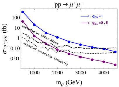
Figure 8: Naive constraint on $\sigma(pp\to\mu^{+}\mu^{-})$ for $\theta_{D}=0$, $\theta_{L}=\pi/2$ and $g_{\rho L}=0.5,1$, where the latest experimental result provided by the ATLAS group is obtained from Ref. ATLAS-CONF-2017-027 . The regions above the black dashed (black dotted) lines are excluded (expected to be excluded after a $300\,\text{fb}^{-1}$ integrated luminosity accumulation) at $95\%$ C.L.s.

In Fig. 8, we show the collider bound for the $\theta_{L}=\pi/2$ case from the dimuon searches. It indicates that our scenario was already tested and excluded up to $m_{\rho}=4\,(1.5)\,\text{TeV}$ at $95\%$ C.L. when $g_{\rho L}=1\,(0.5)$. We should keep in mind, however, that the present scenario with $g_{\rho L}=1$ for the mass range $4\,\text{TeV}\lesssim m_{\rho}\lesssim 10\,\text{TeV}$ can still accommodate the $b\to s\mu^{+}\mu^{-}$ anomaly as seen in Eq.(4.34). Note that the dijet bound for the $\theta_{L}=\pi/2$ case is not significant when $g_{\rho L}<1$.

6 Summary

In this paper, we analyzed the flavorful composite physics of composite vector bosons arising from the one-family model of the vectorlike HC theory, which we dubbed the HC rho model formulated based on the HLS construction. The model structure has been unambiguously fixed by the “chiral” symmetry for the HC fermions and the HLS gauge invariance. The model involves the 63 HC rho mesons and 63 HC pions with phenomenologically rich structure, which couple to the SM gauge bosons as the essential consequence of the HLS gauge invariance. Coupling properties to the SM fermions are restricted due to the HLS gauge invariance of the vectorlike theory. The flavor-dependent couplings are required to be the third-generation fermion-philic by the flavor-dependent EW precision measurements. The flavor-universal couplings, on the other hand, hardly get limited by the EW sector constraints (oblique corrections), which is indeed due to the vectorlike model construction. To be specific, we have found that the forward-backward asymmetry of tau lepton $A_{\rm FB}^{(0,\tau)}$ and the $Z$ boson decay to bottom quark pair $(R_{b})$ are fairly sensitive to the flavor-dependent couplings of the HC rho mesons.

In turn, we surveyed the allowed coupling parameter space of the HC rho mesons from the relevant flavor observables by taking into account the flavor mixing structures between the second and third generations involved in the left-handed down-quarks and leptons, parametrized by the angle $\theta_{D}$ and $\theta_{L}$ as in Eq.(4.2). The most stringent bound come from the $B^{0}_{s}$-$\bar{B}^{0}_{s}$ mixing. In conjunction with other flavor observables, it has turned out that the down-quark mixing $\theta_{D}$ has to be much tiny (but non-zero) while the lepton mixing $\theta_{L}$ has wider allowed range depending on the mass scale of HC rho mesons and the coupling strength as seen in Fig. 1. In particular, the viable scenarios are classified into two spots with respect to $\theta_{L}$: one class is the case that the HC rho mesons predominantly couple to third-generation leptons $(\theta_{L}\lesssim\pi/4)$, and another is to the second-generation ($\theta_{L}\sim\pi/2$), as obtained in Figs. 1 – 3. The exclusion plots combined with the flavor-dependent EW precision tests for the above two cases are shown in Fig. 4. Of interest for both two scenarios is that the HC rho mesons hardly contribute to $B\to D^{(*)}\ell\bar{\nu}$, which in turn implies that the ratios $R_{D^{(*)}}$ do not significantly deviate from the SM predictions. This is essentially because of the almost complete degeneracy in the HC rho mass spectra due to the large flavor-universal coupling ($g_{\rho}\sim 6$). In contrast, the HC rho mesons with mass of TeV scale can give significant contributions to $b\to s\mu^{+}\mu^{-}$. Hence the present scenario can achieve the large values of the Wilson coefficients for the effective operators of $b\to s\mu^{+}\mu^{-}$ with the $V-A$ form ($C_{9}=-C_{10}$), which can account for the present anomalies in the experimental data from LHCb, Belle, ATLAS, and CMS.

We then discussed the implications to the collider physics at LHC and found that the HC rho mesons with mass of TeV scale can be consistent with the current 13 TeV LHC data: In the case with $\theta_{L}\lesssim\pi/4$, the most stringent limit comes from dijet and ditau channels, which turns out to exclude the mass up to $\sim 1-2$ TeV for the flavored HC rho coupling $g_{\rho L}=1-2$ [Fig. 7]. The HC rhos in the other case with $\theta\sim\pi/2$ is, on the other hand, more severely constrained by the dimuon channel, and the mass has already been excluded up to $\sim 4\,(1.5)$ TeV for $g_{\rho L}=1\,(0.5)$.

Thus, our HC rho model has interesting correlations sensitive to the EW precision measurements, the $B$-decay anomalies and the LHC collider signatures. Through the present anatomy of our model, we can reach a definite conclusion: if the current $R_{D^{(*)}}$ anomaly goes away, but the $R_{K^{(*)}}$ deficit further grows to be explained by the flavorful HC rhos on TeV mass scale, then those HC rhos will show up also in the future LHC data on the ditau, dijet and dimuon channels with higher luminosity. In particular, the case with $\theta_{L}\sim\pi/2$ is the most intriguing even when viewed from any point of EW precision, flavor and collider physics; (i) the experimental bound for $b\to s\mu^{+}\mu^{-}$ anomaly can easily be satisfied if and only if a tiny $\theta_{D}$ is at hand, while the case with $\theta_{L}\lesssim\pi/4$ is barely allowed within the $3\sigma$ range even for the tiny $\theta_{D}$ if $g_{\rho}g_{L}^{33}\,(=g_{\rho L})$ is close to unity [Fig. 2]; (ii) the EW precision tests give the severer constraint on the HC rho mass when the $68\%$ C.L. bound is taken into account in the case with $\theta_{L}\lesssim\pi/4$, which is much milder in the case with $\theta_{L}\sim\pi/2$ [Fig. 4]; (iii) the dimuon channel search at the LHC generically has higher sensitivity than the ditau channel, so does the case with $\theta_{L}\sim\pi/2$ [Figs. 7 and 8].

It is also interesting to note that the net effects on the flavor observables in the present model are similar to those in a low-energy effective $U(1)^{\prime}$ model, in spite of the fact that our model includes 63 components of new vector bosons. This can be checked by looking at the analytic formulae for the observables presented in this paper. To be specific, the $U(1)^{\prime}$ model can be described, in terms of the HC rho model, by replacing the coefficient of the four-fermion operators $(\bar{q}_{L}\gamma^{\mu}q_{L})(\bar{q}_{L}\gamma_{\mu}q_{L})$, $(\bar{q}_{L}\gamma^{\mu}q_{L})(\bar{\ell}_{L}\gamma_{\mu}\ell_{L})$, $(\bar{\ell}_{L}\gamma^{\mu}\ell_{L})(\bar{\ell}_{L}\gamma_{\mu}\ell_{L})$: $\frac{7}{16}\frac{g_{\rho}(g_{L}^{33})^{2}}{m_{\rho}^{2}}\to\frac{g_{a}^{33}g_{b}^{33}}{m_{Z^{\prime}}^{2}}$ [for $(a,b)=(q,q),(q,\ell),(\ell,\ell)$], see e.g., Ref. Cline:2017lvv and c.f., Eqs.(4.17), (4.21), (4.23), (4.25), (4.28). Therefore, the HC rho model can be considered as one of the UV completed models that realize the extended $U(1)^{\prime}$ gauge symmetry to the SM at the low energy scale. Unlike the $U{(1)}^{}$

References

- (1) ATLAS collaboration, G. Aad et al., Observation of a new particle in the search for the Standard Model Higgs boson with the ATLAS detector at the LHC, Phys. Lett. B716 (2012) 1–29, [1207.7214].
- (2) CMS collaboration, S. Chatrchyan et al., Observation of a new boson with mass near 125 GeV in pp collisions at = 7 and 8 TeV, JHEP 06 (2013) 081, [1303.4571].
- (3) C. Kilic, T. Okui and R. Sundrum, Vectorlike Confinement at the LHC, JHEP 02 (2010) 018, [0906.0577].
- (4) R. Pasechnik, V. Beylin, V. Kuksa and G. Vereshkov, Chiral-symmetric technicolor with standard model Higgs boson, Phys. Rev. D88 (2013) 075009, [1304.2081].
- (5) P. Lebiedowicz, R. Pasechnik and A. Szczurek, Search for technipions in exclusive production of diphotons with large invariant masses at the LHC, Nucl. Phys. B881 (2014) 288–308, [1309.7300].
- (6) R. Pasechnik, V. Beylin, V. Kuksa and G. Vereshkov, Composite scalar Dark Matter from vector-like confinement, Int. J. Mod. Phys. A31 (2016) 1650036, [1407.2392].
- (7) Lattice Strong Dynamics (LSD) collaboration, T. Appelquist et al., Composite bosonic baryon dark matter on the lattice: SU(4) baryon spectrum and the effective Higgs interaction, Phys. Rev. D89 (2014) 094508, [1402.6656].
- (8) Y. Hochberg, E. Kuflik, H. Murayama, T. Volansky and J. G. Wacker, Model for Thermal Relic Dark Matter of Strongly Interacting Massive Particles, Phys. Rev. Lett. 115 (2015) 021301, [1411.3727].
- (9) T. Appelquist et al., Stealth Dark Matter: Dark scalar baryons through the Higgs portal, Phys. Rev. D92 (2015) 075030, [1503.04203].
- (10) T. Appelquist et al., Detecting Stealth Dark Matter Directly through Electromagnetic Polarizability, Phys. Rev. Lett. 115 (2015) 171803, [1503.04205].
- (11) A. Carmona and M. Chala, Composite Dark Sectors, JHEP 06 (2015) 105, [1504.00332].
- (12) Y. Hochberg, E. Kuflik and H. Murayama, SIMP Spectroscopy, JHEP 05 (2016) 090, [1512.07917].
- (13) K. Harigaya and Y. Nomura, Light Chiral Dark Sector, Phys. Rev. D94 (2016) 035013, [1603.03430].
- (14) A. Kamada, M. Yamada, T. T. Yanagida and K. Yonekura, SIMP from a strong U(1) gauge theory with a monopole condensation, Phys. Rev. D94 (2016) 055035, [1606.01628].
- (15) G. D. Kribs and E. T. Neil, Review of strongly-coupled composite dark matter models and lattice simulations, Int. J. Mod. Phys. A31 (2016) 1643004, [1604.04627].
- (16) L. Forestell, D. E. Morrissey and K. Sigurdson, Non-Abelian Dark Forces and the Relic Densities of Dark Glueballs, Phys. Rev. D95 (2017) 015032, [1605.08048].
- (17) X. Calmet, Seesaw induced Higgs mechanism, Eur. Phys. J. C28 (2003) 451–454, [hep-ph/0206091].
- (18) H. D. Kim, Electroweak symmetry breaking from SUSY breaking with bosonic see-saw mechanism, Phys. Rev. D72 (2005) 055015, [hep-ph/0501059].
- (19) N. Haba, N. Kitazawa and N. Okada, Invisible technicolor, Acta Phys. Polon. B40 (2009) 67–74, [hep-ph/0504279].
- (20) O. Antipin, M. Redi and A. Strumia, Dynamical generation of the weak and Dark Matter scales from strong interactions, JHEP 01 (2015) 157, [1410.1817].
- (21) N. Haba, H. Ishida, N. Okada and Y. Yamaguchi, Bosonic seesaw mechanism in a classically conformal extension of the Standard Model, Phys. Lett. B754 (2016) 349–352, [1508.06828].
- (22) N. Haba, H. Ishida, N. Kitazawa and Y. Yamaguchi, A new dynamics of electroweak symmetry breaking with classically scale invariance, Phys. Lett. B755 (2016) 439–443, [1512.05061].
- (23) H. Ishida, S. Matsuzaki and Y. Yamaguchi, Invisible axionlike dark matter from the electroweak bosonic seesaw mechanism, Phys. Rev. D94 (2016) 095011, [1604.07712].
- (24) H. Ishida, S. Matsuzaki and Y. Yamaguchi, Bosonic-Seesaw Portal Dark Matter, 1610.07137.
- (25) H. Ishida, S. Matsuzaki, S. Okawa and Y. Omura, Scalegenesis via dynamically induced multiple seesaws, 1701.00598.
- (26) N. Haba and T. Yamada, Strong dynamics in a classically scale invariant extension of the Standard Model with flatland, 1701.02146.
- (27) N. Haba and T. Yamada, Multiple-point principle realized with strong dynamics, 1703.04235.
- (28) T. Hur, D.-W. Jung, P. Ko and J. Y. Lee, Electroweak symmetry breaking and cold dark matter from strongly interacting hidden sector, Phys. Lett. B696 (2011) 262–265, [0709.1218].
- (29) T. Hur and P. Ko, Scale invariant extension of the standard model with strongly interacting hidden sector, Phys. Rev. Lett. 106 (2011) 141802, [1103.2571].
- (30) M. Heikinheimo, A. Racioppi, M. Raidal, C. Spethmann and K. Tuominen, Physical Naturalness and Dynamical Breaking of Classical Scale Invariance, Mod. Phys. Lett. A29 (2014) 1450077, [1304.7006].
- (31) M. Holthausen, J. Kubo, K. S. Lim and M. Lindner, Electroweak and Conformal Symmetry Breaking by a Strongly Coupled Hidden Sector, JHEP 12 (2013) 076, [1310.4423].
- (32) S. Abel and A. Mariotti, Novel Higgs Potentials from Gauge Mediation of Exact Scale Breaking, Phys. Rev. D89 (2014) 125018, [1312.5335].
- (33) J. Kubo, K. S. Lim and M. Lindner, Electroweak Symmetry Breaking via QCD, Phys. Rev. Lett. 113 (2014) 091604, [1403.4262].
- (34) O. Antipin, E. Mølgaard and F. Sannino, Higgs Critical Exponents and Conformal Bootstrap in Four Dimensions, JHEP 06 (2015) 030, [1406.6166].
- (35) C. D. Carone and R. Ramos, Dark chiral symmetry breaking and the origin of the electroweak scale, Phys. Lett. B746 (2015) 424–429, [1505.04448].
- (36) J. Kubo and M. Yamada, Genesis of electroweak and dark matter scales from a bilinear scalar condensate, Phys. Rev. D93 (2016) 075016, [1505.05971].
- (37) H. Hatanaka, D.-W. Jung and P. Ko, AdS/QCD approach to the scale-invariant extension of the standard model with a strongly interacting hidden sector, JHEP 08 (2016) 094, [1606.02969].
- (38) E. Molgaard and F. Sannino, Phases of (Asymptotically) Safe Chiral Theories with(out) Scalars, 1610.03130.
- (39) S. Abel and F. Sannino, Radiative symmetry breaking from interacting UV fixed points, 1704.00700.
- (40) M. Bando, T. Kugo, S. Uehara, K. Yamawaki and T. Yanagida, Is rho Meson a Dynamical Gauge Boson of Hidden Local Symmetry?, Phys. Rev. Lett. 54 (1985) 1215.
- (41) M. Bando, T. Kugo and K. Yamawaki, On the Vector Mesons as Dynamical Gauge Bosons of Hidden Local Symmetries, Nucl. Phys. B259 (1985) 493.
- (42) M. Bando, T. Fujiwara and K. Yamawaki, Generalized Hidden Local Symmetry and the A1 Meson, Prog. Theor. Phys. 79 (1988) 1140.
- (43) M. Bando, T. Kugo and K. Yamawaki, Nonlinear Realization and Hidden Local Symmetries, Phys. Rept. 164 (1988) 217–314.
- (44) M. Harada and K. Yamawaki, Hidden local symmetry at loop: A New perspective of composite gauge boson and chiral phase transition, Phys. Rept. 381 (2003) 1–233, [hep-ph/0302103].
- (45) S. Descotes-Genon, T. Hurth, J. Matias and J. Virto, Optimizing the basis of observables in the full kinematic range, JHEP 05 (2013) 137, [1303.5794].
- (46) S. Descotes-Genon, J. Matias and J. Virto, Understanding the Anomaly, Phys. Rev. D88 (2013) 074002, [1307.5683].
- (47) W. Altmannshofer and D. M. Straub, New Physics in ?, Eur. Phys. J. C73 (2013) 2646, [1308.1501].
- (48) G. Hiller and M. Schmaltz, and future physics beyond the standard model opportunities, Phys. Rev. D90 (2014) 054014, [1408.1627].
- (49) W. Altmannshofer and D. M. Straub, New physics in transitions after LHC run 1, Eur. Phys. J. C75 (2015) 382, [1411.3161].
- (50) B. Gripaios, M. Nardecchia and S. A. Renner, Composite leptoquarks and anomalies in -meson decays, JHEP 05 (2015) 006, [1412.1791].
- (51) C. Niehoff, P. Stangl and D. M. Straub, Violation of lepton flavour universality in composite Higgs models, Phys. Lett. B747 (2015) 182–186, [1503.03865].
- (52) C. Niehoff, P. Stangl and D. M. Straub, Direct and indirect signals of natural composite Higgs models, JHEP 01 (2016) 119, [1508.00569].
- (53) A. Carmona and F. Goertz, Lepton Flavor and Nonuniversality from Minimal Composite Higgs Setups, Phys. Rev. Lett. 116 (2016) 251801, [1510.07658].
- (54) R. Barbieri, C. W. Murphy and F. Senia, B-decay Anomalies in a Composite Leptoquark Model, Eur. Phys. J. C77 (2017) 8, [1611.04930].
- (55) G. D’Amico, M. Nardecchia, P. Panci, F. Sannino, A. Strumia, R. Torre et al., Flavour anomalies after the measurement, 1704.05438.
- (56) Y. Sakaki, M. Tanaka, A. Tayduganov and R. Watanabe, Testing leptoquark models in , Phys. Rev. D88 (2013) 094012, [1309.0301].
- (57) B. Dumont, K. Nishiwaki and R. Watanabe, LHC constraints and prospects for scalar leptoquark explaining the anomaly, Phys. Rev. D94 (2016) 034001, [1603.05248].
- (58) A. Datta, M. Duraisamy and D. Ghosh, Diagnosing New Physics in decays in the light of the recent BaBar result, Phys. Rev. D86 (2012) 034027, [1206.3760].
- (59) A. Celis, M. Jung, X.-Q. Li and A. Pich, Sensitivity to charged scalars in and decays, JHEP 01 (2013) 054, [1210.8443].
- (60) A. Crivellin, A. Kokulu and C. Greub, Flavor-phenomenology of two-Higgs-doublet models with generic Yukawa structure, Phys. Rev. D87 (2013) 094031, [1303.5877].
- (61) I. Doršner, S. Fajfer, N. Košnik and I. Nišandžić, Minimally flavored colored scalar in and the mass matrices constraints, JHEP 11 (2013) 084, [1306.6493].
- (62) M. Freytsis, Z. Ligeti and J. T. Ruderman, Flavor models for , Phys. Rev. D92 (2015) 054018, [1506.08896].
- (63) N. G. Deshpande and X.-G. He, Consequences of R-parity violating interactions for anomalies in and , Eur. Phys. J. C77 (2017) 134, [1608.04817].
- (64) M. A. Ivanov, J. G. Körner and C.-T. Tran, Analyzing new physics in the decays with form factors obtained from the covariant quark model, Phys. Rev. D94 (2016) 094028, [1607.02932].
- (65) W. Altmannshofer, P. S. B. Dev and A. Soni, anomaly: A possible hint for natural supersymmetry with -parity violation, 1704.06659.
- (66) A. H. Fariborz, R. Jora and J. Schechter, Global aspects of the scalar meson puzzle, Phys. Rev. D79 (2009) 074014, [0902.2825].
- (67) LatKMI collaboration, Y. Aoki et al., Light flavor-singlet scalars and walking signals in QCD on the lattice, 1610.07011.
- (68) M. Tanabashi, Chiral perturbation to one loop including the rho meson, Phys. Lett. B316 (1993) 534–541, [hep-ph/9306237].
- (69) S. Matsuzaki and K. Yamawaki, Walking on the ladder: 125 GeV technidilaton, or Conformal Higgs, JHEP 12 (2015) 053, [1508.07688].
- (70) H. S. Fukano, S. Matsuzaki, K. Terashi and K. Yamawaki, Conformal Barrier and Hidden Local Symmetry Constraints: Walking Technirhos in LHC Diboson Channels, Nucl. Phys. B904 (2016) 400–447, [1510.08184].
- (71) H. S. Fukano, M. Kurachi, S. Matsuzaki, K. Terashi and K. Yamawaki, 2 TeV Walking Technirho at LHC?, Phys. Lett. B750 (2015) 259–265, [1506.03751].
- (72) J. Wess and B. Zumino, Consequences of anomalous Ward identities, Phys. Lett. 37B (1971) 95–97.
- (73) E. Witten, Global Aspects of Current Algebra, Nucl. Phys. B223 (1983) 422–432.
- (74) W. Buchmuller, R. Ruckl and D. Wyler, Leptoquarks in Lepton - Quark Collisions, Phys. Lett. B191 (1987) 442–448.
- (75) R. Barbieri, A. Pomarol and R. Rattazzi, Weakly coupled Higgsless theories and precision electroweak tests, Phys. Lett. B591 (2004) 141–149, [hep-ph/0310285].
- (76) M. E. Peskin and T. Takeuchi, Estimation of oblique electroweak corrections, Phys. Rev. D46 (1992) 381–409.
- (77) R. S. Chivukula, E. H. Simmons, H.-J. He, M. Kurachi and M. Tanabashi, Universal non-oblique corrections in Higgsless models and beyond, Phys. Lett. B603 (2004) 210–218, [hep-ph/0408262].
- (78) SLD Electroweak Group, DELPHI, ALEPH, SLD, SLD Heavy Flavour Group, OPAL, LEP Electroweak Working Group, L3 collaboration, S. Schael et al., Precision electroweak measurements on the resonance, Phys. Rept. 427 (2006) 257–454, [hep-ex/0509008].
- (79) Particle Data Group collaboration, C. Patrignani et al., Review of Particle Physics, Chin. Phys. C40 (2016) 100001.
- (80) B. Bhattacharya, A. Datta, J.-P. Guv́in, D. London and R. Watanabe, Simultaneous Explanation of the and Puzzles: a Model Analysis, 1609.09078.
- (81) C. Bobeth, M. Gorbahn, T. Hermann, M. Misiak, E. Stamou and M. Steinhauser, in the Standard Model with Reduced Theoretical Uncertainty, Phys. Rev. Lett. 112 (2014) 101801, [1311.0903].
- (82) S. Descotes-Genon, J. Matias, M. Ramon and J. Virto, Implications from clean observables for the binned analysis of at large recoil, JHEP 01 (2013) 048, [1207.2753].
- (83) LHCb collaboration, R. Aaij et al., Measurement of Form-Factor-Independent Observables in the Decay , Phys. Rev. Lett. 111 (2013) 191801, [1308.1707].
- (84) LHCb collaboration, R. Aaij et al., Angular analysis of the decay using 3 fb-1 of integrated luminosity, JHEP 02 (2016) 104, [1512.04442].
- (85) Belle collaboration, A. Abdesselam et al., Angular analysis of , in Proceedings, LHCSki 2016 - A First Discussion of 13 TeV Results: Obergurgl, Austria, April 10-15, 2016, 2016. 1604.04042.
- (86) Belle collaboration, S. Wehle et al., Lepton-Flavor-Dependent Angular Analysis of , Phys. Rev. Lett. 118 (2017) 111801, [1612.05014].
- (87) ATLAS Collaboration collaboration, Angular analysis of decays in collisions at TeV with the ATLAS detector, Tech. Rep. ATLAS-CONF-2017-023, CERN, Geneva, Apr, 2017.
- (88) CMS Collaboration collaboration, Measurement of the and angular parameters of the decay in proton-proton collisions at , Tech. Rep. CMS-PAS-BPH-15-008, CERN, Geneva, 2017.
- (89) LHCb collaboration, R. Aaij et al., Differential branching fraction and angular analysis of the decay , JHEP 07 (2013) 084, [1305.2168].
- (90) LHCb collaboration, R. Aaij et al., Angular analysis and differential branching fraction of the decay , JHEP 09 (2015) 179, [1506.08777].
- (91) LHCb collaboration, R. Aaij et al., Test of lepton universality using decays, Phys. Rev. Lett. 113 (2014) 151601, [1406.6482].
- (92) S. Bifani (on behalf of the LHCb collaboration), Search for new physics with decays at LHCb, tech. rep., 18 Apr 2017.
- (93) B. Capdevila, S. Descotes-Genon, J. Matias and J. Virto, Assessing lepton-flavour non-universality from angular analyses, JHEP 10 (2016) 075, [1605.03156].
- (94) B. Capdevila, A. Crivellin, S. Descotes-Genon, J. Matias and J. Virto, Patterns of New Physics in transitions in the light of recent data, 1704.05340.
- (95) W. Altmannshofer, P. Stangl and D. M. Straub, Interpreting Hints for Lepton Flavor Universality Violation, 1704.05435.
- (96) L.-S. Geng, B. Grinstein, S. Jäger, J. Martin Camalich, X.-L. Ren and R.-X. Shi, Towards the discovery of new physics with lepton-universality ratios of decays, 1704.05446.
- (97) M. Ciuchini, A. M. Coutinho, M. Fedele, E. Franco, A. Paul, L. Silvestrini et al., On Flavourful Easter eggs for New Physics hunger and Lepton Flavour Universality violation, 1704.05447.
- (98) G. Hiller and I. Nisandzic, and beyond the Standard Model, 1704.05444.
- (99) A. Celis, J. Fuentes-Martin, A. Vicente and J. Virto, Gauge-invariant implications of the LHCb measurements on Lepton-Flavour Non-Universality, 1704.05672.
- (100) A. K. Alok, D. Kumar, J. Kumar and R. Sharma, Lepton flavor non-universality in the B-sector: a global analyses of various new physics models, 1704.07347.
- (101) A. K. Alok, B. Bhattacharya, A. Datta, D. Kumar, J. Kumar and D. London, New Physics in after the Measurement of , 1704.07397.
- (102) W. Wang and S. Zhao, Implications of the and anomalies, 1704.08168.
- (103) BaBar collaboration, J. P. Lees et al., Search for and invisible quarkonium decays, Phys. Rev. D87 (2013) 112005, [1303.7465].
- (104) Belle collaboration, O. Lutz et al., Search for with the full Belle data sample, Phys. Rev. D87 (2013) 111103, [1303.3719].
- (105) A. J. Buras, J. Girrbach-Noe, C. Niehoff and D. M. Straub, decays in the Standard Model and beyond, JHEP 02 (2015) 184, [1409.4557].
- (106) Belle collaboration, Y. Miyazaki et al., Search for Lepton-Flavor-Violating tau Decays into a Lepton and a Vector Meson, Phys. Lett. B699 (2011) 251–257, [1101.0755].
- (107) K. Hayasaka et al., Search for Lepton Flavor Violating Tau Decays into Three Leptons with 719 Million Produced Tau+Tau- Pairs, Phys. Lett. B687 (2010) 139–143, [1001.3221].
- (108) Heavy Flavor Averaging Group (HFAG) collaboration, Y. Amhis et al., Averages of -hadron, -hadron, and -lepton properties as of summer 2014, 1412.7515.
- (109) BaBar collaboration, J. P. Lees et al., Measurement of an Excess of Decays and Implications for Charged Higgs Bosons, Phys. Rev. D88 (2013) 072012, [1303.0571].
- (110) Belle collaboration, M. Huschle et al., Measurement of the branching ratio of relative to decays with hadronic tagging at Belle, Phys. Rev. D92 (2015) 072014, [1507.03233].
- (111) LHCb collaboration, R. Aaij et al., Measurement of the ratio of branching fractions , Phys. Rev. Lett. 115 (2015) 111803, [1506.08614].
- (112) Belle collaboration, S. Hirose et al., Measurement of the lepton polarization and in the decay , 1612.00529.
- (113) J. Charles et al., Current status of the Standard Model CKM fit and constraints on New Physics, Phys. Rev. D91 (2015) 073007, [1501.05013].
- (114) S. Aoki et al., Review of lattice results concerning low-energy particle physics, Eur. Phys. J. C74 (2014) 2890, [1310.8555].
- (115) S. Aoki et al., Review of lattice results concerning low-energy particle physics, 1607.00299.
- (116) J. Jia, S. Matsuzaki and K. Yamawaki, Walking technipions at the LHC, Phys. Rev. D87 (2013) 016006, [1207.0735].
- (117) S. Matsuzaki and K. Yamawaki, 750 GeV Diphoton Signal from One-Family Walking Technipion, Mod. Phys. Lett. A31 (2016) 1630016, [1512.05564].
- (118) O. Kaymakcalan, S. Rajeev and J. Schechter, Nonabelian Anomaly and Vector Meson Decays, Phys. Rev. D30 (1984) 594.
- (119) R. P. Kauffman and W. Schaffer, QCD corrections to production of Higgs pseudoscalars, Phys. Rev. D49 (1994) 551–554, [hep-ph/9305279].
- (120) R. Franceschini, G. F. Giudice, J. F. Kamenik, M. McCullough, A. Pomarol, R. Rattazzi et al., What is the resonance at 750 GeV?, JHEP 03 (2016) 144, [1512.04933].
- (121) ATLAS collaboration, T. A. collaboration, Search for scalar diphoton resonances with 15.4 fb-1 of data collected at =13 TeV in 2015 and 2016 with the ATLAS detector, .
- (122) CMS collaboration, V. Khachatryan et al., Search for high-mass diphoton resonances in proton–proton collisions at 13 TeV and combination with 8 TeV search, Phys. Lett. B767 (2017) 147–170, [1609.02507].
- (123) M. Harada, M. Kurachi and K. Yamawaki, Meson masses in large N(f) QCD from Bethe-Salpeter equation, Phys. Rev. D68 (2003) 076001, [hep-ph/0305018].
- (124) M. Kurachi and R. Shrock, Study of the Change from Walking to Non-Walking Behavior in a Vectorial Gauge Theory as a Function of N(f), JHEP 12 (2006) 034, [hep-ph/0605290].
- (125) LSD collaboration, T. Appelquist et al., Lattice simulations with eight flavors of domain wall fermions in SU(3) gauge theory, Phys. Rev. D90 (2014) 114502, [1405.4752].
- (126) ATLAS collaboration, G. Aad et al., Search for Scalar Diphoton Resonances in the Mass Range GeV with the ATLAS Detector in Collision Data at = 8 , Phys. Rev. Lett. 113 (2014) 171801, [1407.6583].
- (127) ATLAS collaboration, M. Aaboud et al., Search for scalar leptoquarks in pp collisions at = 13 TeV with the ATLAS experiment, New J. Phys. 18 (2016) 093016, [1605.06035].
- (128) CMS collaboration, A. M. Sirunyan et al., Search for dijet resonances in proton-proton collisions at sqrt(s) = 13 TeV and constraints on dark matter and other models, Phys. Lett. B (2016) , [1611.03568].
- (129) CMS collaboration, V. Khachatryan et al., Search for heavy resonances decaying to tau lepton pairs in proton-proton collisions at TeV, JHEP 02 (2017) 048, [1611.06594].
- (130) T. Han, Collider phenomenology: Basic knowledge and techniques, in Physics in . Proceedings, Theoretical Advanced Study Institute in elementary particle physics, TASI 2004, Boulder, USA, June 6-July 2, 2004, pp. 407–454, 2005. hep-ph/0508097.
- (131) J. Pumplin, D. R. Stump, J. Huston, H. L. Lai, P. M. Nadolsky and W. K. Tung, New generation of parton distributions with uncertainties from global QCD analysis, JHEP 07 (2002) 012, [hep-ph/0201195].
- (132) D. B. Clark, E. Godat and F. I. Olness, ManeParse: a Mathematica reader for Parton Distribution Functions, 1605.08012.
- (133) J. H. Friedman, A Nested Partitioning Procedure for Numerical Multiple Integration and Adaptive Importance Sampling, ACM Trans. Math. Software 7 (1981) 76.
- (134) J. H. Friedman and M. H. Wright, DIVONNE4: A PROGRAM FOR MULTIPLE INTEGRATION AND ADAPTIVE IMPORTANCE SAMPLING, .
- (135) T. Hahn, CUBA: A Library for multidimensional numerical integration, Comput. Phys. Commun. 168 (2005) 78–95, [hep-ph/0404043].
- (136) J. Alwall, M. Herquet, F. Maltoni, O. Mattelaer and T. Stelzer, MadGraph 5 : Going Beyond, JHEP 06 (2011) 128, [1106.0522].
- (137) J. Alwall, R. Frederix, S. Frixione, V. Hirschi, F. Maltoni, O. Mattelaer et al., The automated computation of tree-level and next-to-leading order differential cross sections, and their matching to parton shower simulations, JHEP 07 (2014) 079, [1405.0301].
- (138) C. Degrande, C. Duhr, B. Fuks, D. Grellscheid, O. Mattelaer and T. Reiter, UFO - The Universal FeynRules Output, Comput. Phys. Commun. 183 (2012) 1201–1214, [1108.2040].
- (139) N. D. Christensen and C. Duhr, FeynRules - Feynman rules made easy, Comput. Phys. Commun. 180 (2009) 1614–1641, [0806.4194].
- (140) A. Alloul, N. D. Christensen, C. Degrande, C. Duhr and B. Fuks, FeynRules 2.0 - A complete toolbox for tree-level phenomenology, Comput. Phys. Commun. 185 (2014) 2250–2300, [1310.1921].
- (141) R. Brun and F. Rademakers, ROOT: An object oriented data analysis framework, Nucl. Instrum. Meth. A389 (1997) 81–86.
- (142) ATLAS collaboration, M. Aaboud et al., Search for new phenomena in dijet events using 37 fb-1 of collision data collected at 13 TeV with the ATLAS detector, 1703.09127.
- (143) ATLAS Collaboration collaboration, Search for new high-mass phenomena in the dilepton final state using 36.1 fb-1 of proton-proton collision data at 13 TeV with the ATLAS detector, Tech. Rep. ATLAS-CONF-2017-027, CERN, Geneva, Apr, 2017.
- (144) J. M. Cline, J. M. Cornell, D. London and R. Watanabe, Hidden sector explanation of -decay and cosmic ray anomalies, Phys. Rev. D95 (2017) 095015, [1702.00395].
- (145) S. Matsuzaki, K. Nishiwaki and R. Watanabe, work in progress.
- (146) R. Contino, The Higgs as a Composite Nambu-Goldstone Boson, in Physics of the large and the small, TASI 09, proceedings of the Theoretical Advanced Study Institute in Elementary Particle Physics, Boulder, Colorado, USA, 1-26 June 2009, pp. 235–306, 2011. 1005.4269. DOI.
- (147) B. Bellazzini, C. Csáki and J. Serra, Composite Higgses, Eur. Phys. J. C74 (2014) 2766, [1401.2457].
- (148) G. Panico and A. Wulzer, The Composite Nambu-Goldstone Higgs, Lect. Notes Phys. 913 (2016) pp.1–316, [1506.01961].
- (149) R. Barbieri, D. Buttazzo, F. Sala and D. M. Straub, Flavour physics from an approximate symmetry, JHEP 07 (2012) 181, [1203.4218].
- (150) R. Barbieri, G. Isidori, A. Pattori and F. Senia, Anomalies in -decays and flavour symmetry, Eur. Phys. J. C76 (2016) 67, [1512.01560].
- (151) A. R. Vidal (on behalf of the LHCb collaboration), Lepton Flavour Universality tests using semitauonic decays at LHCb, tech. rep., 6 June 2017.
- (152) V. D. Barger and R. J. N. Phillips, COLLIDER PHYSICS. 1987.