Berezinskii-Kosterlitz-Thouless transition and criticality of an elliptic deformation of the sine-Gordon model

Abstract

We introduce and study the properties of a periodic model interpolating between the sine– and the sinh–Gordon theories in $1+1$ dimensions. This model shows the peculiarities, due to the preservation of the functional form of their potential across RG flows, of the two limiting cases: the sine-Gordon, not having conventional order/magnetization at finite temperature, but exhibiting Berezinskii-Kosterlitz-Thouless (BKT) transition; and the sinh-Gordon, not having a phase transition, but being integrable. The considered interpolation, which we term as sn-Gordon model, is performed with potentials written in terms of Jacobi functions. The critical properties of the sn-Gordon theory are discussed by a renormalization-group approach. The critical points, except the sinh-Gordon one, are found to be of BKT type. Explicit expressions for the critical coupling as a function of the elliptic modulus are given.

I Introduction

Symmetries and dimensionality play a crucial role in the determination of critical properties and phase diagrams. As an example, in quantum field theory one of the most studied model is the Ising one with interaction terms $\varphi^{4}$ which is known to have two phases in $d=1+1$ dimensions in one of which the $Z_{2}$ symmetry has been broken spontaneously giuseppe . Another paradigmatic and well studied instance of phase transition in $d=2$ dimensions is provided by the sine-Gordon (sG) scalar theory where the interaction Lagrangian contains a periodic self-interaction $\cos{(\beta\varphi)}$. The sG model has been widely studied for the properties of its soliton solutions drazin ; raja and it is known to exhibit a Berezinskii-Kosterlitz-Thouless (BKT) phase transition minnhagen87 ; kadanoff . Replacing the real valued frequency $\beta$ of the sG model by an imaginary one, $\beta\to i\beta$, one arrives at the sinh-Gordon (shG) model with a self-interaction term $\cos{(i\beta\varphi)}=\cosh{(\beta\varphi)}$ which is in turn a well studied scalar field theory giuseppe .

For the shG model the periodicity is lost and no BKT type transition is expected. One could argue that, due to its non-periodic nature, the interaction potential can be expanded in Taylor series which generates $\varphi^{2N}$ terms, so that one could very naively expect an Ising type phase structure. However, this is not the case. The shG model is known to possess a single phase, and the explanation of this fact is related to the preservation of the functional form of its potential doreybook , which is connected with the special properties of the exponentials entering the hyperbolic functions.

Another way to relate the Ising, sG and shG models is based on their conformal properties. It is known that systems at criticality, where they are scale-invariant, may give rise to invariance under the larger group of conformal transformations polyakov_1970 locally acting as scale transformations di_francesco_1997 . The conformal symmetry in $d=2$ dimensions encloses infinitely many local transformations di_francesco_1997 and its occurrence and consequences for $2$-dimensional field theories have been deeply investigated and exploited to obtain a variety of exact results di_francesco_1997 ; giuseppe . As a consequence of conformal invariance the central charge $c$ is well defined at any fixed point in the phase structure of the model and its difference $\Delta c$ between the one at the Gaussian and the non-trivial fixed point characterizes the theory. In case of the Ising model, $\Delta c\equiv c_{\mathrm{UV}}-c_{\mathrm{IR}}=1/2$ where the high-energy (UV) value $c_{\mathrm{UV}}$ is taken at the Gaussian while the low-energy (IR) value $c_{\mathrm{IR}}$ is chosen at the Wilson-Fisher fixed points. It is known that $\Delta c=1/2$, $1$, $1$ for the Ising, sG and shG models respectively. It is clear that the peculiarities of the sG and shG models based on the preservation of the functional form of its potential along renormalization group (RG) flows are at the basis of the fact that in both cases $\Delta c=1$, with the result for the shG model differing from that of the Ising although it is not periodic.

The goal of the present work is to introduce and discuss a class of models interpolating between the sG and the shG models. The critical properties of the proposed models can be studied by functional RG, which allows as well to clarify from the point of view of the interpolation the characteristics of the shG model discussed above. The used RG technique is well suited to undercover the critical properties, at least at qualitative level, of field theoretical models, since it maintains the full functional form of the effective potential under study. This property has proven necessary in order to achieve accurate results for $O(N)$ field theories in any real dimension and with generic non analytic kinetic terms in the effective action Defenu2015a ; Defenu2015 ; Defenu2016 .

The interpolation considered in this paper, that we term sn-Gordon (snG) model, is based on Jacobi functions byrd . We remind that the definition of the Jacobi functions follows the same line as the $\sin$ and $\cos$ functions, but considering the unit ellipse, rather than the unit circle as the geometrical object to be described. Denoting $x,y$ the two coordinates in the $\mathbb{R}^{2}$ space, all the points of an ellipse with eccentricity $m$ can be parametrised by

$$x=r\cos(\theta),\,\,y=r\sin(\theta),\,\,r =\frac{1}{\sqrt{1-m^{2}\sin(\theta)^{2}}}$$ (1)

where $\theta$ is the angle in the $x-y$ plane. Starting from this definition one can define the Jacopi amplitude, i.e. the angular arc length of the ellipse

$$u(\theta,m)=\int_{0}^{\theta}\frac{d\omega}{1-m^{2}\sin^{2}(\omega)}.$$ (2)

Rephrasing the relations in Eq. (1) in terms of the two variables $u,m$ and proceeding in analogy with the trigonometric case one gets to the following definitions

$$x=\frac{{\mathrm{cn}}(u,m)}{{\mathrm{dn}}(u,m)},\quad y=\frac{{\mathrm{sn}}(u,m)}{{\mathrm{dn}}(u,m)},\quad r=\frac{1}{{\mathrm{dn}}(u,m)}$$ (3)

for the fundamental Jacobi functions.

In order to introduce the considered interpolation we preliminarly observe that the Jacobi functions ${\mathrm{sn}}(\beta\varphi,m)$, ${\mathrm{cn}}(\beta\varphi,m)$ reduces respectively to $\sin(\beta\varphi)$, $\cos(\beta\varphi)$ for vanishing elliptic modulus ($m=0$) and to $\tanh(\beta\varphi)$, $1/\cosh(\beta\varphi)$ for $m=1$. Indeed, in the $m\to 1$ limit, the eccentricity is unity and the ellipse, described by Eqs. (1), becomes a parabola. As a consequence the functions in Eq. (3) cannot be periodic, since they do not represent a closed curve. Therefore, a simple interpolating model with a potential expressed in terms of Jacobi functions can be constructed as

$$V_{{\mathrm{snG}}}(\varphi)=u\,{\mathrm{cn}}(\beta\varphi,m)=u\,{\mathrm{cd}}(\beta\varphi,m)\,{\mathrm{nd}}(\beta\varphi,m).$$ (4)

where ${\mathrm{nd}}(\beta\varphi,m)=1/{\mathrm{dn}}(\beta\varphi,m)$ and ${\mathrm{cd}}(u,m)={\mathrm{cn}}(u,m)/{\mathrm{dn}}(u,m)$. The snG potential (4) for $m=0$ reads $u\cos(\beta\varphi)$, while for $m=1$ it is $u\cosh(\beta\varphi)$ reducing to the shG potential $V_{{\mathrm{shG}}}$. We observe that the interpolating potential is periodic (except for $m=1$) and we therefore do expect a BKT transition for $0\leq m<1$.

Figure 1: The snG potential $V_{{\mathrm{snG}}}(\varphi)$ as a function of $\varphi$ for $u=1$ with $m=(0,0.85,0.99,1)$ from bottom to top respectively while we set $\beta\equiv 1$. Note that the $m=0$ case (lightest grey curve) is equivalent to the sine-Gordon potential $V_{sG}(\varphi)=u\cos(\varphi)$, while the darkest curve for $m=1$ becomes non-periodic and represents the sinh-Gordon potential $V_{shG}(\varphi)=u\cosh(\varphi)$

An important comment is that, while the sG and the shG models are integrable both at classical and quantum level, models interpolating between them are in general not integrable (we refer to Olshanetsky1981 ; Olshanetsky1983 for a discussion of $1+1$ classical and quantum integrable models). In the case considered in the present paper, (4) provides an elliptic interpolation between the sG and the shG model, deforming/generalizing the sG potential with $m$ being the deformation parameter. We observe that suitable elliptic deformations can be integrable, as one can see in one-dimensional non-relativistic systems of classical particles interacting via a potential given by a Weierstrass function which reduces to potentials of the form $1/\sin^{2}(x)$ and $1/\sinh^{2}(x)$, where $x$ is the distance between the two particles Olshanetsky1981 . Another example is provided by integrable elliptic generalizations of the Calogero model Langmann2014 . In this paper we will not deal with the, actually very interesting, problem of constructing integrable elliptic deformations of the sG model and to study their soliton-like solutions, but we are primarily interested in introducing a generalization of the sG model interpolating between the sG itself and the shG to study the BKT transition across the interpolation between these two paradigmatic models. From this point of view the parametrization (4) represents one of the simplest one can think of and suitable to study critical BKT transitions in elliptically deformed models.

The approach followed here, with the interpolation inserted via the potential (4) in the Lagrangian, is different from the models in which the interpolation is done directly in the $S$-matrix, as the staircase model in which an analytic continuation of the shG $S$-matrix is performed to describe interpolating flows between minimal models in $2D$ Zamolodchikov2006 . These interpolating models, studied in relation to the so-called “roaming”, are integrable by construction. In the staircase model a real parameter $\theta_{0}$ encodes the distance of the continued $S$-matrix from the shG self-dual point: in the limit of large $\theta_{0}$, the ground-state energy found by thermodynamic Bethe ansatz exhibits a sequence of scaling behaviours approximating those of the minimal conformal field theories. Several aspects of staircase and related models were studied martins92 ; dorey93 ; ahn1993 ; delfino95 ; delfino96 ; Dorey2015 ; Horvath16 , including a study of the form factors of the shG field fring when the real parameter $\theta_{0}$ is sent to infinity ahn1993 (see more references in Horvath16 ). In these models one typically does not work with the Lagrangian (and to reconstruct the Lagrangian corresponding to their $S$-matrices is not straightforward) – at variance the model with the snG potential (4) defines a bare Lagrangian, but anyway one can ask the fate of RG flow in the interpolation between sG and shG models.

Finally let us mention an example of interpolation done at the Lagrangian level by considering the coupling constant $\beta=\beta_{1}+i\beta_{2}$ as a complex quantity, where $\beta_{1}$ and $\beta_{2}$ are real value frequencies. We note that the resulting class of theories can be treated for each non-zero $\beta_{2}$ as a scalar polynomial field theory and denoted as as the Shine-Gordon model. Since we are interested mainly in the study of BKT universality class we stick to model (4), while model with $\beta=\beta_{1}+i\beta_{2}$ could be studied in relation to the roaming phenomena. Finally, we observe that a $(2+1)$ integrable interpolation between the sG and the shG models has been already proposed in Pempinelli1987 , while in brane-world gravity context a modification of the shG model has been considered Mannheim2005 .

A disclaimer here, before going in medias res, is certainly due. As mentioned in raja , the convention of denoting the generalization of the Klein-Gordon model to sinusoidal potential as “sine-Gordon” generated a certain amount of controversy. If from this point of view the proliferation of similar abbreviations should be avoided, from the other the use of sine-Gordon and sinh-Gordon models has become so widespread both in physics and mathematics literature that in this paper devoted to Lagrangian interpolation between these two limits we decided for the purpose of compactness to refer to the model (4) as sn-Gordon.

The paper is organized as follows. Section II is devoted to introduce the functional RG formalism for the study of the snG model. We also discuss there the linearized RG equations. In Section III we discuss in detail the limiting cases of the snG corresponding to shG and sG. We use functional RG to discuss also how the standard results are retrieved in these two cases, including the point that the shG model does not have a phase transition and the subtleties of the $m\to 1$ limit. The discussion of Section III provides the basis for our main results exposed in Section IV where we give the functional RG treatment of the snG and we discuss the critical properties and the critical values of the coupling $\beta$ as a function of the deformation parameter, the elliptic modulus m. Section V is devoted to our conclusions.

II Linearized RG equations for the sn-Gordon model

In this section we briefly summarize the functional RG approach for scalar models, and its application to the shG and the snG models.

The functional RG equation has the following form We1993 ; Morris94 ; Berges02 ; Polony04 ; Delamotte12

$$k\partial_{k}\Gamma_{k}[\varphi]=\frac{1}{2}{\mathrm{Tr}}\left[\frac{k\partial_{k}R_{k}}{\Gamma^{(2)}_{k}[\varphi]+R_{k}}\right]$$ (5)

for the effective action $\Gamma_{k}[\varphi]$. $\Gamma^{(2)}_{k}[\varphi]$ denotes the second functional derivative of the effective action and the trace ${\mathrm{Tr}}$ stands for the integration over all momenta. The RG equation (5) is a functional equation, that should be handled by truncations. Truncated RG flows depend on the choice of the regulator function $R_{k}$, i.e. on the renormalization scheme. Regulator functions have already been discussed in the literature by introducing its dimensionless form

$$R_{k}(p)=p^{2}r(y),\hskip 14.22636pty=p^{2}/k^{2},$$

where $r(y)$ is dimensionless. Various types of regulator functions can be chosen, but a general choice is the so called CSS regulator css ; css_sg which recovers all major types of regulators in appropriate limits: the Litim opt_rg , the power-law Mo1994 and the exponential We1993 ones. The mass cutoff is the power-law regulator $r(y)=y^{-b}$ with $b=1$.

We observe that we do not include the wavefunction renormalization in the definition of the regulator when using truncations beyond the leading order of the derivative expansion (see below). In this case, in order to ensure scale-invariance one has to use the power-law regulator. While this is certainly a restriction we take this choice in order to be able to rely on previous results, see e.g., sG_Trun .

One of the commonly used systematic approximation is the truncated derivative expansion where the action is expanded in powers of the derivative of the field,

$$\Gamma_{k}[\varphi]=\int_{x}\left[V_{k}(\varphi)+Z_{k}(\varphi)\frac{1}{2}(\partial_{\mu}\varphi)^{2}+...\right].$$

In the so called Local Potential Approximation (LPA), higher derivative terms are neglected and the wave-function renormalization is set equal to constant, i.e. $Z_{k}\equiv 1$. In this case (5) reduces to the partial differential equation for the dimensionless blocked potential ($\tilde{V}_{k}=k^{-2}V_{k}$) which has the following form for $d=2$ dimensions

$$(2+k\partial_{k}){\tilde{V}}_{k}(\varphi)=-\frac{1}{4\pi}\int_{0}^{\infty}dy\frac{y^{2}\frac{dr}{dy}}{(1+r)y+{\tilde{V}^{\prime\prime}}_{k}(\varphi)},$$ (6)

where ${\tilde{V}^{\prime\prime}}_{k}(\varphi)$ is the second derivative of the potential with respect to the field.

Before going into the details of the solution of the exact functional RG equation, in this section we take the linearized form (around the Gaussian fixed point) of the equation (6) obtained in the LPA level which reads as

$$(2+k\partial_{k}){\tilde{V}}_{k}(\varphi)=-\frac{1}{4\pi}{\tilde{V}^{\prime\prime}}_{k}(\varphi)+{\cal O}(\tilde{V}^{\prime\prime 2}_{k}),$$ (7)

independently of the choice of the regulator functions $r(y)$ and apply it to the Ising, sG, shG and to the interpolating snG models.

For periodic models which undergo a BKT type phase transition the linearised RG equation at LPA can be used to determine the exact value of the critical frequency $\beta^{2}_{c}$ which separates the phases of the model. This is a unique property of sG type models based on the fact that (i) the ”critical” fixed point where $\beta^{2}_{c}$ is calculated situates at vanishing Fourier amplitude, (ii) the RG flow equation obtained for the wavefunction renormalization beyond the linearised and LPA levels (see e.g., Eq. (III.2)) has no linear dependence on the Fourier amplitude, thus, for small amplitudes it has no scale-dependence at all, hence the exact critical frequency can be obtained by the LPA linearised RG equation (7).

II.1 The Ising model

Although it is not the goal of the present work to consider the functional RG study of the Ising model, since it is useful in the following let us first apply (7) for the Ising model by substituting

$$\tilde{V}_{{\mathrm{Ising}}}(\varphi)=\sum_{n=1}^{{\mathrm{N_{CUT}}}}\frac{\tilde{g}_{2n}(k)}{(2n)!}\varphi^{2n},$$ (8)

into Eq. (7). One can then read the RG flow equations for the scale dependent dimensionless couplings $\tilde{g}_{2n}(k)$. For any finite ${\mathrm{N_{CUT}}}$, the linearized functional RG equation does not preserve the functional form of the bare theory (8), i.e., the l.h.s of (7) contains polynomial terms $\varphi^{2n}$ of order $n={\mathrm{N_{CUT}}}$. The r.h.s of (7) has terms of order $n<{\mathrm{N_{CUT}}}$. Let us note that the same holds for the case where the linearization of the functional RG equation (6) is performed in terms of the field-dependent part of $V^{\prime\prime}_{k}(\varphi)$ which results in a regulator-dependent linearized functional RG equation.

II.2 The sG model

The situation is different for the sG model where the bare potential is defined by (for the sake of simplicity keeping only the fundamental Fourier mode)

$$\tilde{V}_{{\mathrm{sG}}}(\varphi)=\tilde{u}_{k}\cos(\beta\varphi),$$ (9)

where the dimensionless Fourier amplitude carries the scale-dependence since in LPA the frequency $\beta$ does not depend on the running momentum cutoff $k$. It is clear that the linearized functional RG equation (7) preserve the functional form of the bare potential (no higher harmonics are generated):

$$(2+k\partial_{k})\tilde{u}_{k}\cos(\beta\varphi)=\frac{1}{4\pi}\beta^{2}\tilde{u}_{k}\cos(\beta\varphi).$$ (10)

The RG flow equation for the Fourier amplitude reads

$$k\partial_{k}\tilde{u}_{k}=\tilde{u}_{k}\left(-2+\frac{1}{4\pi}\beta^{2}\right),$$ (11)

with a solution

$$\tilde{u}_{k}=\tilde{u}_{\Lambda}\left(\frac{k}{\Lambda}\right)^{-2+\frac{\beta^{2}}{4\pi}}$$ (12)

which determines the critical frequency $\beta_{c}^{2}=8\pi$, where the model undergoes a BKT-type phase transition coleman . It is important to note that even if the bare theory of the sG model contains higher harmonics, the linearized functional RG equation (7) reduces to decoupled flow equations for the Fourier amplitudes of various modes.

II.3 The shG model

By using the replacement $\beta\to i\beta$ in Eq. (9), one finds the bare potential for the shG model

$$\tilde{V}_{{\mathrm{shG}}}(\varphi)=\tilde{u}_{k}\cos(i\beta\varphi)=\tilde{u}_{k}\cosh(\beta\varphi)$$ (13)

which is inserted into (7) preserving again the functional form of the bare potential:

$$(2+k\partial_{k})\tilde{u}_{k}\cosh(\beta\varphi)=-\frac{1}{4\pi}\beta^{2}\tilde{u}_{k}\cosh(\beta\varphi).$$ (14)

The RG flow equation for the Fourier amplitude reads

$$k\partial_{k}\tilde{u}_{k}=\tilde{u}_{k}\left(-2-\frac{1}{4\pi}\beta^{2}\right),$$ (15)

with a solution

$$\tilde{u}_{k}=\tilde{u}_{\Lambda}\left(\frac{k}{\Lambda}\right)^{-2-\frac{\beta^{2}}{4\pi}},$$ (16)

showing that in case of $\beta^{2}=8\pi$ the exponent does not change sign, hence, the shG model has no BKT-type phase transition. In other words, the linearized functional RG of the shG model can be derived from the sG model by using the replacement $\beta\to i\beta$ which results in a sign change of $\beta^{2}$ and no BKT-type phase transition.

II.4 The snG model

In the snG model, the dimensionless bare potential reads

$$\tilde{V}_{{\mathrm{snG}}}(\varphi)=\tilde{A}_{k}\,{\mathrm{cd}}(\beta\varphi,m)\,{\mathrm{nd}}(\beta\varphi,m),$$ (17)

where the amplitude $\tilde{A}_{k}$ is scale-dependent. By using the properties of the Jacobi functions ${\mathrm{cd}}(u,m)={\mathrm{cn}}(u,m)/{\mathrm{dn}}(u,m)$ and ${\mathrm{nd}}(u,m)=1/{\mathrm{dn}}(u,m)$ it can also be written as

$$\tilde{V}_{{\mathrm{snG}}}(\varphi)=\tilde{A}_{k}\,{\mathrm{cn}}(\beta\varphi,m)\,[{\mathrm{nd}}(\beta\varphi,m)]^{2}.$$ (18)

Inserting Eq. (17) or Eq. (18) into the linearized functional RG equation (7) one observes that the functional form is not preserved since the second derivatives of the potential has the following form

$$\tilde{V}^{\prime\prime}_{{\mathrm{snG}}}(\varphi) = \beta^{2}\tilde{A}_{k}\frac{{\mathrm{cn}}(\beta\varphi,m)}{{\mathrm{dn}}(\beta\varphi,m)^{4}}$$

$$\left(6(m-1)+(5-4m)\,{\mathrm{dn}}(\beta\varphi,m)^{2}\right).$$

However, it is important to note that the Jacobi function (17) is a periodic function, so, it can be expanded in Fourier series. One has

$${\mathrm{cn}}(u,m) = \frac{2\pi}{K\sqrt{m}}\sum_{n=0}^{\infty}\frac{q^{n+1/2}}{1+q^{2n+1}}\cos\left[(2n+1)\frac{\pi u}{2K}\right],$$

$${\mathrm{nd}}(u,m) = \frac{\pi}{2K\sqrt{1-m}}$$

$$+ \frac{2\pi}{K\sqrt{1-m}}\sum_{n=1}^{\infty}\frac{(-1)^{n}q^{n}}{1+q^{2n}}\cos\left[2n\frac{\pi u}{2K}\right],$$

where $q=\exp[-\pi K(1-m)/K(m)]$ and $K(m)$ is the quarter period which can be expressed by the hypergeometric function

$$K=\int_{0}^{\pi/2}\frac{d\theta}{\sqrt{1-m\,\sin^{2}(\theta)}}=\frac{\pi}{2}\,\,{}_{2}F_{1}\left(\frac{1}{2},\frac{1}{2},1,m\right).$$

It follows then

$$\tilde{V}_{{\mathrm{snG}}}(\varphi)=\sum_{n=1}^{\infty}\tilde{u}_{n}(k)\cos(n\,b\,\varphi),\,\,b=\frac{\beta}{{}_{2}F_{1}\left(\frac{1}{2},\frac{1}{2},1,m\right)}.$$ (19)

Inserting (19) into the linearized functional RG equation (7), one can derive a set of uncoupled differential equations for the Fourier modes

$$k\partial_{k}\tilde{u}_{n}(k)=\tilde{u}_{n}(k)\left(-2+\frac{1}{4\pi}n^{2}b^{2}\right).$$ (20)

Similarly to the sG model the critical frequency corresponds to the fundamental mode, i.e., for $n=1$ where one finds $b_{c}^{2}=8\pi$ and the higher harmonics do not modify it nandori_sg ; schemes . Thus, one can read the $m$-dependence of the original frequency

$$\beta_{c}^{2}(m)=8\pi\,\left[{}_{2}F_{1}\left(\frac{1}{2},\frac{1}{2},1,m\right)\right]^{2}$$ (21)

which clearly signals the existence of a BKT-type phase transition if $m\neq 1$. In the limit $m\to 0$ one gets back $\beta_{c}^{2}=8\pi$, while for $m\to 1$ the original frequency blows up and the model has a single phase. Thus, the $m=1$ case the snG model undergoes no BKT phase transition.

However, at this stage we would like to pay the attention of the reader to the following important observation. In the limit $m\to 1$ the snG models reduces to the shG theory, thus, it is important to study whether the information obtained from the snG model for $m\to 1$ is in agreement with the results on the shG model. The grey area of Fig. 2 stands for the so called massive phase, where the fundamental Fourier amplitude is increasing in the IR limit, so it is expected that the shG model has to have a single phase with the same properties. We will show in the next section that indeed, the shG model does not undergo any phase transitions. The question which needs to be clarified is whether this single phase of the shG model share all features of the massive phase of the snG model and whether to what extent the limit $m\to 1$ is singular. We shall come back on the limit $m\to 1$ in the next section.

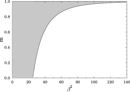
Figure 2: Phase structure of the snG model in the $m,\beta^{2}$ plane based on Eq. (21) indicating a BKT-type phase transition for $m\neq 1$ where the grey area stands for the massive phase.

In summary, one can conclude that the sG and shG models have a special structure such that their functional forms are preserved by the linearized functional RG equation. A BKT-type phase transition is observed for the sG and the snG models, for the latter with a condition $m\neq 1$.

III Functional RG equations

Here we consider the study of the models introduced in the previous section. The functional RG equations are taken in LPA for the Ising model with ${\mathrm{N_{CUT}}}=2$ and beyond LPA for the other models (keeping only the fundamental mode).

III.1 Ising model

Here we repeat briefly the functional RG study of the Ising model where apart from the trivial mass term, a $\varphi^{4}$ self-interaction is taken into account ($N_{\rm CUT}=2$). The functional RG equations are taken in the LPA level, reading in $d=2$ dimensions as

$$\partial_{t}g_{2}=-2g_{2}-\frac{1}{4\pi}\frac{g_{4}}{(1+g_{2})}$$ (22)

$$\partial_{t}g_{4}=-2g_{4}+\frac{3}{4\pi}\frac{g_{4}^{2}}{(1+g_{2})^{2}}$$ (23)

for the mass cutoff and

$$\partial_{t}g_{2}=-2g_{2}-\frac{1}{4\pi}\frac{g_{4}}{(1+g_{2})^{2}}$$ (24)

$$\partial_{t}g_{4}=-2g_{4}+\frac{6}{4\pi}\frac{g_{4}^{2}}{(1+g_{2})^{3}}$$ (25)

for the Litim cutoff. The above equations have a trivial Gaussian and a non-trivial (cutoff-dependent) Wilson-Fisher (WF) fixed point, where the latter indicates the existence of two phases. The $c$-function along the trajectory starting at the Gaussian and terminating at the WF fixed points is known to decrease by $\Delta c=1/2$. However, if one consider the massive deformation of the Gaussian fixed point $\Delta c=1$ c_theorem ; c_func .

III.2 sG model

If the sG model (9) is studied beyond LPA, the RG equation has to be solved over the functional subspace spanned by the following ansatz

$$\Gamma_{k}=\int d^{2}x\left[\frac{1}{2}z_{k}(\partial_{\mu}\varphi)^{2}+V_{k}(\varphi)\right],$$ (26)

where the local potential contains a single Fourier mode

$$V_{k}(\varphi)=-u_{k}\cos(\varphi),$$ (27)

and the following notation is introduced

$$z_{k}\equiv 1/\beta^{2}$$ (28)

via the rescaling of the field $\varphi\to\varphi/\beta$ in (9), with $z_{k}$ the field-independent wave-function renormalization. Then Eq. (5) leads to the evolution equations for the coupling constants sG_Trun ,

$$k\partial_{k}u_{k} = \frac{1}{2\pi}\int_{p}~{}\frac{(k\partial_{k}R_{k})}{u_{k}}\left(\frac{P_{k}}{\sqrt{P_{k}^{2}-u_{k}^{2}}}-1\right),$$ (29)

$$k\partial_{k}z_{k} = \frac{1}{2\pi}\int_{p}(k\partial_{k}R_{k})\biggl{(}\frac{u_{k}^{2}p^{2}(\partial_{p^{2}}P_{k})^{2}(4P_{k}^{2}+u_{k}^{2})}{4(P_{k}^{2}-u_{k}^{2})^{7/2}}$$ (30)

$$-\frac{u_{k}^{2}P_{k}(\partial_{p^{2}}P_{k}+p^{2}\partial_{p^{2}}^{2}P_{k})}{2(P_{k}^{2}-u_{k}^{2})^{5/2}}\biggr{)}$$

with $P_{k}=z_{k}p^{2}+R_{k}$. In general, the momentum integrals have to be performed numerically, however, in some cases analytical results are available. Indeed, by using the mass cutoff, i.e. power-law type regulator with $b=1$, the momentum integrals can be performed and the RG equations reads as,

$$(2+k\partial_{k}){\tilde{u}}_{k} = \frac{1}{2\pi z_{k}{\tilde{u}}_{k}}\left[1-\sqrt{1-{\tilde{u}}_{k}^{2}}\right]$$

$$k\partial_{k}z_{k} = -\frac{1}{24\pi}\frac{{\tilde{u}}_{k}^{2}}{[1-{\tilde{u}}_{k}^{2}]^{\frac{3}{2}}}$$ (31)

with the dimensionless coupling ${\tilde{u}}=k^{-2}u$. The phase structure of the sG model based on Eqs. (III.2) is plotted on Fig. 3 which indicates two phases with a critical value for the frequency $\beta_{c}^{2}=8\pi$.

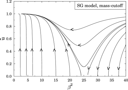
Figure 3: Phase structure of the sG model based on Eqs. (III.2) indicating a BKT-type phase transition with $\beta_{c}^{2}=8\pi$.

Let us note that the power-law regulator with $b=1$, i.e., the mass cutoff has poor convergence properties (RG trajectories does not reach the IR fixed point in the weak coupling phase), but its advantage that the momentum integral can be calculated analytically. A better result can be obtained by using for example $b=2$, as shown in c_func_sg .

III.3 shG model

It is important to note that (13) has a $Z_{2}$ symmetry, and that the shG model is not periodic. Therefore, in order to study the RG flow of the shG model and to map out its phase structure one can use the Taylor-expanded form of Eq. (13)

$$\tilde{V}_{k}(\varphi) = \tilde{u}_{k}\left[1+\frac{1}{2}\beta^{2}\varphi^{2}+\frac{1}{4!}\beta^{4}\varphi^{4}+...\right]$$ (32)

$$= \sum_{n=0}^{\infty}\frac{1}{(2n)!}g_{2n}\varphi^{2n},\hskip 14.22636ptg_{2n}=\tilde{u}_{k}\beta^{2n}.$$

Thus, the shG model can be considered as an Ising-type model but with restricted initial values for the couplings. The key point is that with shG-type initial values the RG flow always starts from the symmetric phase, see Fig. 4. Therefore, the shG model has a single phase, so, it does not go through a BKT or other type of phase transitions.

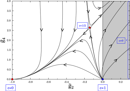
Figure 4: Representation of the shG model in the $g_{2},g_{4}$ plane based on its Taylor expansion (32). The shaded area stands for initial conditions for the shG model which indicates a single phase.

The shG model has a special structure that no $2\to 2n$ particle production is allowed, i.e. the production amplitudes of any $2$ particles decay into $2n$ ones are zero at tree-level (and also at 1-loop level) giuseppe ; doreybook . This special structure of the bare Lagrangian of the shG model results in a single phase.

The phase structure of the shG model can also be mapped out by using analytic continuation. The simplest way of doing that if one try the replacement of the frequency by an imaginary one directly. For example, the RG flow equations for the shG model can be constructed from (III.2)

$$(2+k\partial_{k})\tilde{u}_{k} = -\frac{\beta^{2}}{2\pi\tilde{u}_{k}}\left[1-\sqrt{1-\tilde{u}_{k}^{2}}\right]$$ (33)

$$k\partial_{k}\beta_{k}^{2} = -\frac{1}{24\pi}\frac{\beta_{k}^{4}\tilde{u}_{k}^{2}}{[1-\tilde{u}_{k}^{2}]^{\frac{3}{2}}}.$$ (34)

The RG flow of the shG model based on (33) and (34) is obtained numerically and shown in Fig. 5 which also indicates a single phase for the shG model. We observe that due to the poor convergence properties of the regulator ($b=1$ power-law), similarly to the sG case, the RG trajectories do not converge properly, specially in the limit of vanishing $\beta^{2}$.

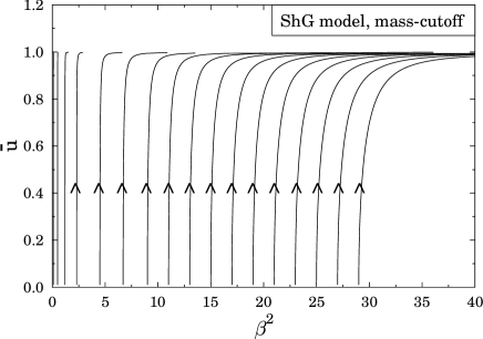
Figure 5: Phase structure of the shG model based on (33) and (34) indicates a single phase.

Let us now turn to the study of the $c$-function for the shG model. In our previous paper c_func_sg we worked out a proper treatment of the $c$-function for the sG scalar theory in the framework of functional RG. In the limit of vanishing frequency, the shG and sG models become identical to each other, thus the method of c_func_sg can be applied here for the shG model using the following parametrization

$$\tilde{V}_{k}(\varphi)=\frac{\tilde{m}_{k}^{2}}{\beta^{2}}\left(\cos(i\beta\varphi)-1\right),$$ (35)

where the frequency $\beta$ is assumed to be scale-dependent. In the limit $\beta\to 0$, the RG equations for the special form of the shG model (35) reduce to

$$k\partial_{k}\tilde{m}_{k}^{2} \approx \frac{\tilde{m}_{k}^{2}[-\beta^{2}-8\pi(1+\tilde{m}_{k}^{2})]}{4\pi(1+\tilde{m}_{k}^{2})}\approx-2\tilde{m}_{k}^{2}$$ (36)

$$k\partial_{k}\beta^{2} = 0.$$ (37)

Following the method discussed in c_func_sg , the $c$-function of the shG model can be determined in the framework of functional RG based on the flow equations (36) and (37) which is identical to that of the sG model in the limit of $\beta\to 0$. Thus, the flows for the $c$-function of the shG and the sG models are identical in the limit of vanishing frequency, consequently they give us the same result which recovers the known value $\Delta c=1$ ($\Delta c=c_{UV}-c_{IR}$) c_func_sg .

Finally, we briefly discuss on the issue of analytic continuation of the sG theory for imaginary frequencies. If one replaces the real value frequency by an imaginary one then the action of the sG model becomes that of the shG theory. This means that one can apply the following replacement $\beta^{2}\to-\beta^{2}$ in the flow equations of the sG theory in order to obtain the flow equations for the shG model. Indeed, the flow diagram of the shG model is plotted in Fig. 5. This result can be visualised in a different way, i.e., by extending the sG flow diagram for negative value of the frequency $\beta^{2}$, see Fig. 6, which can be compared to figure 1 of Ref. malard . There is a disagreement between the two figures, namely in malard the RG trajectories of the negative $\beta^{2}$ regime run into the IR (convexity) fixed point of the sG model which signals the presence of spontaneous symmetry breaking (SSB). At variance, we argued in this paper that the shG model has no SSB, since it has a single phase which is the symmetric one. Moreover, the flow diagram plotted in figure 1 of malard suggests that the negative and positive $\beta^{2}$ regions are basically reflected to each other, implying in turn the reflection of the critical value of the frequency ($\beta_{c}^{2}=8\pi$) too. However, it was also shown here that no such critical frequency exists for the shG model i.e., the negative $\beta^{2}$ case of the sG theory. Therefore, we conclude that figure 1 of malard may be misleading and we refer to Fig. 6 below.

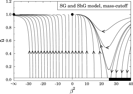
Figure 6: Phase structure of the sG model for regions of positive and negative $\beta^{2}$, i.e., the RG flow diagram of the sG (Fig. 3) and shG (Fig. 5) models are merged into a single one. Black circles denote the IR attractive fixed points.

IV Functional RG study of the snG model

We are now in position to perform the functional RG study of the snG model. According to the previous discussion, it is based on the Fourier decomposition (19) where the frequency $b^{2}$ of the fundamental mode plays a crucial role in the determination of the phase structure. Thus, beyond LPA, the snG model can be treated the way as the sG model, so the RG equation has to be solved over the functional subspace spanned by the following ansatz

$$\Gamma_{k}=\int d^{2}x\left[\frac{1}{2}z_{k}(\partial_{\mu}\varphi_{x})^{2}+V_{k}(\varphi_{x})\right],$$ (38)

where the local potential contains infinitely many Fourier modes

$$V_{k}(\varphi)=-\sum_{n=1}^{\infty}u_{n}(k)\cos(n\,\varphi),$$ (39)

and the following notations are introduced

$$z\equiv\frac{1}{b^{2}}=\frac{\left[{}_{2}F_{1}\left(\frac{1}{2},\frac{1}{2},1,m\right)\right]^{2}}{\beta^{2}}$$ (40)

via the rescaling of the field $\varphi\to\varphi/b$ in (19) and $z_{k}$ again standing for the field-independent wave-function renormalization. It is important to note that $m$ remains a non-scaling parameter even beyond LPA.

In order to follow the strategy done for the sG model one has to take the single-Fourier mode approximation of the snG model (39). The higher harmonics do not change the qualitative picture drawn by the single-Fourier mode approximation (for $m\neq 1$) nandori_sg . Indeed, by using the mass cutoff, i.e., the power-law type regulator with $b=1$, the RG equations for the couplings of the snG reads as,

$$(2+k\partial_{k}){\tilde{u}}_{k} = \frac{1}{2\pi z_{k}{\tilde{u}}_{k}}\left[1-\sqrt{1-{\tilde{u}}_{k}^{2}}\right]$$

$$k\partial_{k}z_{k} = -\frac{1}{24\pi}\frac{{\tilde{u}}_{k}^{2}}{[1-{\tilde{u}}_{k}^{2}]^{\frac{3}{2}}}$$ (41)

with the dimensionless coupling ${\tilde{u}}=k^{-2}u$ which is identical to the flow equations (III.2) of the sG model but with the different definition for $z$. In order to compare the flow diagrams of the snG and sG models it is convenient to use the squared frequency $\beta^{2}$ instead of the wave function renormalization $z$. Then, the flow diagram of the snG model obtained in the single-Fourier approximation beyond LPA for the particular value $m=0.45$ is shown in Fig. 7.

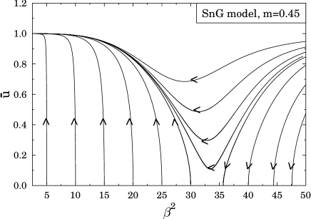
Figure 7: Phase structure of the snG model for $m=0.45$, indicating a BKT-type phase transition with $\beta_{c}^{2}\approx 33.3$.

Fig. 8 is summarizing our results on the critical properties of snG obtained by RG.

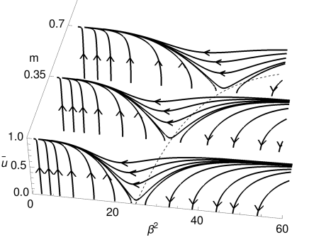
Figure 8: Phase structure of the snG model for $m=0,0.35,0.7$. The dashed line indicates the critical frequency $\beta_{c}^{2}(m)$ of the BKT phase transition, similarly to Fig. 2.

We finally comment on the limit $m\to 1$ of the snG model. We showed that the snG model, being periodic, has a BKT transition in all points but for $m=1$ where it reduces to the shG model. Therefore, let us discuss whether the limit $m\to 1$ is analytic or not. Two facts that would support the analytic behaviour are following: (i) the shG as well as the snG model with $m=1$ show a single phase; (ii) this phase is the high-temperture one, where the Fourier amplitude is relevant. However, in favour of the fact that the limit $m\to 1$ is not analytic one can argue that (i) the frequency is relevant in the shG model, but irrelevant in the $m\to 1$ limit; and (ii) the single phase of the shG model is the symmetric one, but the $m\to 1$ limit suggests SSB. In order to clearly make a conclusion on the subtleties of the $m\to 1$ limit, one has to show a physical quantity which has different value at the two cases. To this purpose we propose to the susceptibility of the topological charge

$$\chi=\langle Q^{2}\rangle-\langle Q\rangle^{2}$$ (42)

where $Q$ is the winding number, see nandori_sg . This serves as a disorder parameter, since the topological susceptibility is vanishing whenever the Fourier amplitude is zero. This quantity can be shown to be non-zero in the limit $m\to 1$ of the snG model, but vanishing for the shG theory. Therefore, we conclude that the limit $m\to 1$ is non analytic.

V Summary

In the present work the renormalization group (RG) study of a class of models interpolating between the sine-Gordon (sG) and the sinh-Gordon (shG) theories has been addressed. The study of the functional RG equations clearly show that only the sG and shG model has a special structure such that their functional forms are preserved by the linearized functional RG equations. It was discussed that functional RG provides a tool to show that while the sG theory undergoes a phase transition at $\beta^{2}=8\pi$, this is absent in the shG model. We argued that the shG model has a single phase since it can be considered as an Ising-type model but with restricted initial values for the coupling constants.

We also studied the proposed model, to which we referred as the sn-Gordon (snG) model, where the potential is expressed in terms of a product of Jacobi functions. We concluded that the snG model exhibits a BKT phase transition for all $m\neq 1$, and we determined the phase diagram and the critical value of $\beta$ as a function of the Jacobi parameter $m$. These results clearly shows the peculiarities of the two limiting cases, the shG and the sG models.

Finally we observe that other interpolations between the sG and the shG models can be considered. In this paper we focused on the critical properties of the snG model, but it would be interesting to study also the solitonic solutions of the snG model and of other possible elliptic interpolations. In view of the connection between the Ruijsenaars-Schneider models Rui86 and the sG model Rui86 ; BabBer , a deserving investigation would be to study the possiblity of integrable interpolations between the sG and the shG models.

References

- (1) G. Mussardo, Statistical field theory: an introduction to exactly solved models in statistical physics (Oxford, Oxford University Press, 2010).
- (2) P. G. Drazin, Solitons (Cambridge, Cambridge University Press, 1983).
- (3) R. Rajaraman, Solitons and instantons: an introduction to solitons and instantons in quantum field theory (Amsterdam, North-Holland, 1987).
- (4) P. Minnhagen, Rev. Mod. Phys. 59, 1001 (1987).
- (5) L. P. Kadanoff, Statistical physics: statics, dynamics and renormalization (Singapore, World Scientific, 2000).
- (6) P. Dorey, in Conformal Field Theories and Integrable Models, Z. Horváth and L. Palla eds., Lecture Notes in Physics Volume 498, pg. 85 (Berlin, Springer-Verlag, 1997).
- (7) A. M. Polyakov, JETP Lett. 12, 381 (1970).
- (8) P. Di Francesco, P. Mathieu, and D. Sénéchal, Conformal Field Theory (New York, Springer, 1997).
- (9) N. Defenu, et al., JHEP 1505 141 (2014).
- (10) N. Defenu, A. Trombettoni, and A. Codello, Phys. Rev. E 92, 052213 (2015).
- (11) N. Defenu, A.Trombettoni, and S. Ruffo, Phys. Rev. B 94, 224411 (2016); ibid. 96, 104432 (2017).
- (12) P. F. Byrd and M. D. Friedman, Handbook of elliptic integrals for engineers and scientists (Berlin, Springer-Verlag, 1971).
- (13) M. A. Olshanetsky and A. M. Perelomov, Phys. Rep. 71, 313 (1981).
- (14) M. A. Olshanetsky and A. M. Perelomov, Phys. Rep. 94, 313 (1983).
- (15) E. Langmann, Ann. Henri Poincare 15, 755 (2014).
- (16) Al. B. Zamolodchikov, J. Phys. A 39, 12847 (2006).
- (17) M. J. Martins, Phys. Rev. Lett. 69, 2461 (1992).
- (18) P. E. Dorey and F. Ravanini, Int. J. Mod. Phys. A 8, 873 (1993); Nucl. Phys. B 406, 708 (1993).
- (19) C. Ahn, G. Delfino, and G. Mussardo, Phys. Lett. B 317, 573 (1993).
- (20) G. Delfino, G. Mussardo, and P. Simonetti, Phys. Rev. D 51, 6620 (1995).
- (21) G. Delfino, P. Simonetti, and J. L. Cardy, Phys. Lett. B 387, 327 (1996).
- (22) P. Dorey, G. Siviour, and G. Takacs, JHEP 1503, 054 (2015).
- (23) D. X. Horvath, P. E. Dorey, and G. Takacs, JHEP 1607, 051 (2016).
- (24) A. Fring, G. Mussardo, and P. Simonetti, Nucl. Phys. B 393, 413 (1993).
- (25) M. Boiti, J. J. P. Leon, and F. Pempinelli, Inverse Probl. 3, 37 (1987).
- (26) P. D. Mannheim, Brane-Localized Gravity (Singapore, World Scientific, 2005).
- (27) C. Wetterich, Nucl. Phys. B 352, 529 (1991); Phys. Lett. B 301, 90 (1993).
- (28) T. R. Morris, Phys. Lett. B 334, 355 (1994).
- (29) J. Berges, N. Tetradis, and C. Wetterich, Phys. Rep. 363, 223 (2002).
- (30) J. Polonyi, Central Eur. J. Phys. 1, 1 (2004).
-
(31)
B. Delamotte, in Order, disorder and criticality:
advanced problems of phase transition theory,
Yu. Holovatch ed. (Singapore, World Scientific, 2007)
[
arXiv:cond-mat/0702365]. - (32) I. Nándori, JHEP 1304, 150 (2013).
- (33) I. Nándori, I. G. Márián, and V. Bacsó, Phys. Rev. D 89, 047701 (2014).
- (34) D. F. Litim, Phys. Lett. B 486, 92 (2000).
- (35) T. R. Morris, Int. J. Mod. Phys. A 9, 2411 (1994).
- (36) S. Nagy, I. Nándori, J. Polonyi, and K. Sailer, Phys. Rev. Lett. 102, 241603 (2009).
- (37) S. Coleman, Phys. Rev. D 11, 2088 (1975).
- (38) I. Nándori, J. Polonyi, and K. Sailer, Phys. Rev. D 63, 045022 (2001).
- (39) I. Nándori, S. Nagy, K. Sailer, and A. Trombettoni, Phys. Rev. D 80, 025008 (2009).
- (40) A. B. Zamolodchikov, JETP Lett. 43, 730 (1986).
- (41) A. Codello, G. D’Odorico, and C. Pagani, JHEP 1407, 040 (2014).
- (42) V. Bacsó, N. Defenu, A. Trombettoni, and I. Nándori, Nucl. Phys. B 901, 444 (2015).
- (43) M. Malard, Braz. J. Phys. 43, 182 (2013).
- (44) S. N. M. Ruijsenaars and H. Schneider, Ann. Phys. (NY) 170, 370 (1986); S. N. M. Ruljsenaars, Commun. Math Phys. 110, 191 (1987).
- (45) O. Babelon and D. Bernard, Phys. Lett. B 317, 363 (1993).