Ipanema-$\beta$ : tools and examples for HEP analysis on GPU

Abstract

1 Introduction

We present here a set of examples, classes and tools which can be used for statistical analysis in Graphics Processing Units (GPU). This includes binned and unbinned maximum likelihood fits, pseudo-experiment generation, convolutions, Markov Chain Monte Carlo method implementations, and limit setting techniques. Our idea is that these examples can be used either as starting points by anyone interested in the subject, or as a framework to develop given analyses. Hence, we include cases with different levels of complexity, starting by showing how to use and combine existing packages, down to more realistic examples that required of us the development of generic classes. Our code is based on pyCUDA [1], which is then combined with scientific packages for analysis such as iMinuit [2, 3] or pyMultinest [4]. In Sect. 2, we list the packages that we use, as well as other approaches we tried or that could be of interest for the reader. Sections 3-7 describe the provided examples. Section 8 is meant to collect some frequently asked questions.

2 Software

The Ipanema package is available on git:

git clone https://gitlab.cern.ch/bsm-fleet/Ipanema.git .

It contains the following folders:

urania cuda polibio examples

and a simple setup.csh script. The software we use depends on the following:

• Cuda. Tested with 7.5 and 8.0.

• Python2 (we used 2.7.11).

• Standard Python packages for scientific usage, such as scipy, numpy, matplotlib. We got them all through an installation of Anaconda [5]. We tested both against Anaconda2 and Anaconda4.

• pyCuda [1] (not in Anaconda). In addition, we made a modified version of curand.py, (toyrand.py) where the generation of an array of poisson numbers uses a separate poisson mean per generated value. We include toyrand.py in the repository.

• reikna [6] (not in Anaconda).

• Default (for likelihood fits): iminuit [2] (not in Anaconda). In order to use analytical gradients, one needs to get the version from the git master branch. If not, then the standard 1.2 is fine.

• Optional, multidimensional parameter sampling: Multinest [7], pymultinest [4] (not in Anaconda).

• Optional, symbolic programing: sympy (included in Anaconda), Mathematica (optional, can be called by urania modules to substitute some of the utilities of sympy).

There are several interesting packages on the market that we don’t use here, but that the reader may be interested in:

• GooFit. This is the software that was shown to us in Rio. It mimics the structure of RooFit, but for Cuda. We don’t use it because we preferred to work mostly from Python, and because at the time we knew about GooFit, there were still functionalitites missing that we needed. It can be used with a related software, Hydra.

• numba.accelerate: It contains an alternative to pyCUDA, which can upload Python fucntions to a GPU using decorators. It was the base of our first attempts to make fitting programs via Python+CUDA. But after some time we moved to pyCUDA instead. We gave it a short try to combine both, but they didn’t seem compatible.

• Faddeeva’s function from GitHub. It is not used in the current released examples, but we are using it for more realistic versions of the $B_{s}^{0}\to{{{J\mskip-3.0mu/\mskip-2.0mu\psi\mskip 2.0mu}}}KK$ fit, for instance.

  To test the examples we provide, we use three graphics card models: GeForce 980 GTX Ti, GeForce 1080 GTX and Tesla M2090. Their specifications are listed in D.

3 Example 1: Fit to a signal peak on top of an exponential background

File: examples/sbfit.py
In this example, a signal peak is fitted on top of an exponential background, using an unbinned maximum likelihood fit. The signal probability density function (PDF) is implemented in a file called psIpatia.cu as a device function, __device__ double log_apIpatia. A __device__ function is only accessible by the GPU. The signal PDF is then processed inside sbfit.py by pyCUDA’s SourceModule. Since SourceModule uses strings, we read psIpatia.cu as:

mod = SourceModule(file("psIpatia.cu","r").read()).

An alternative way is to define a string which contains the CUDA code, as done in the standard pyCUDA examples.

The signal PDF is later called by a global function, __global__ void Ipatia, over an array of data. Global functions are visible both for the GPU and for the host (e.g. a CPU). They must be of type void, meaning that any output has to be passed as an argument. In this case, the output (int_gpu) is an array with the signal PDF value of each data point. The function is then called in Python as:

sig_pdf(bins_gpu, int_gpu, np.float64(mu), np.float64(sigma),
np.float64(l), np.float64(beta), np.float64(a), np.float64(n),
np.float64(a2), np.float64(n2), block = (1000,1,1),
grid = (len(mydat)/1000,1)).

Note that each parameter has to be passed to the GPU using the variable type specified in the CUDA code. In this case, all parameters are of type double, which is passed as np.float64(parameter). The last two arguments of the fuction define the block and grid size in the GPU. The maximum block size depends on the computing capability of the graphics card and is smaller or equal than 1024. The limitations for the grid size are much looser. In this case we are making blocks of 1000 events each, and then the grid as large as needed so that it covers all the events, i.e, $Nevts=block[x]\times grid[x]$. The $y$ and $z$ components of the block/grid are not used.

The minimization is done by Minuit, via the iminuit package. Minuit minimizes a given cost function, FCN. In most of the usages in high-energy physics, the FCN is $-2\log L$ (or just $-\log L$) and a typical definition for fit errors correspond to a change of one unit in $-2\log L$. Inside the FCN the signal and background PDF,

$$\begin{array}[]{lll}\!\!\!\texttt{bkg\_gpu}\!\!\!\!\!&=&\!\!\!\!\!\texttt{pycuda.cumath.exp(k*data\_array\_gpu)},\\ \end{array}$$

and afterwards the likelihood for each data point are calculated in parallel by the GPU,

$$\begin{array}[]{lll}\!\!\!\texttt{LL\_gpu}\!\!\!\!\!&=&\!\!\!\!\!\texttt{pycuda.cumath.log(fs*invint\_s*sig\_gpu+fb*invint\_b*bkg\_gpu)}.\\ \end{array}$$

Here, invint_s and invint_b are the inverses of the signal and background PDF integrals, integral_ipa and integral_exp, respectively. The calculation of integral_ipa is performed numerically by summing up the int_gpu entries,

integral_ipa = np.sum((int_gpu).get())*DM.

The background PDF integral is determined analytically,

if k!= 0 :

integral_exp = (np.exp(k*Mmax)-np.exp(k*Mmin))*1./k

else :

integral_exp = (Mmax - Mmin).

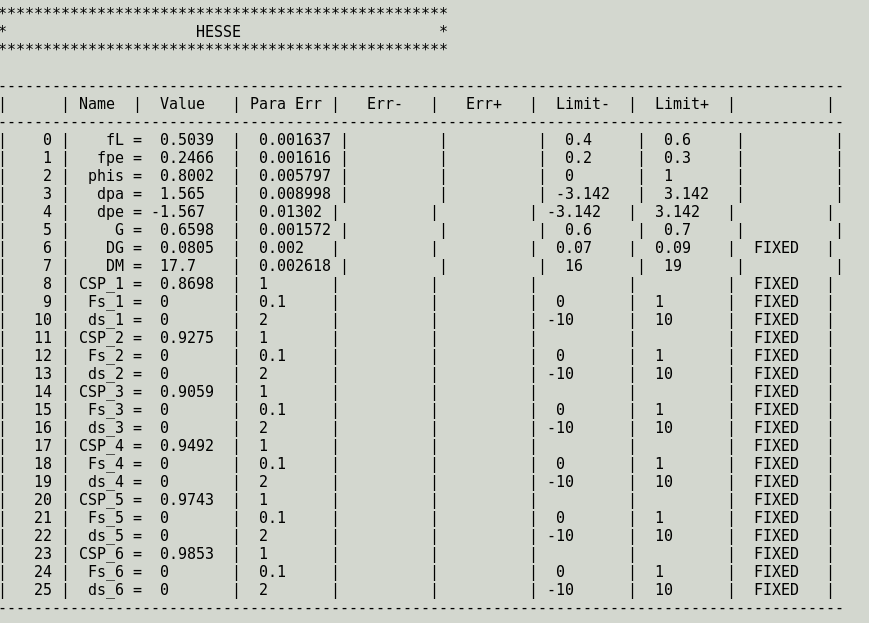
This parallelization significantly reduces the computational time compared to an algorithm which loops over the data and calculates each value in sequence. Note also that some operations, such as the calculation of an exponential or a logarithmic function, can be performed directly on the gpu_array from the Python function even though it is parallelized and executed in the GPU, as shown above. In the end, the individual likelihoods are summed up to a total likelihood in the CPU. The sum, including normalization terms, is returned as the output of FCN. The results of the MIGRAD and HESSE methods and the corresponding correlation matrix are shown in Fig. 1.

Figure 1: Fit result of Example 1: (a) MIGRAD output, (b) HESSE output, (c) parameter correlation matrix.

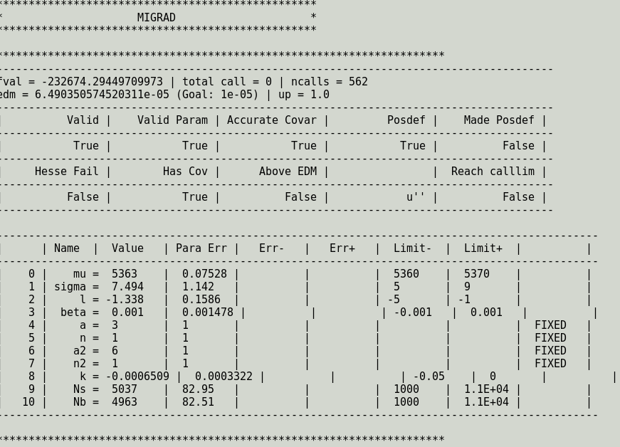
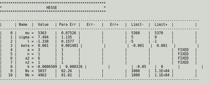
The example prints in the end the GPU time in seconds. We measured the following timings in different devices (Table 1):

Table 1: Timings of Example 1 in different devices (see text for details).

Device	10k events	10M events
	time [s]
GeForce 980 GTX Ti	0.9	30.9
GeForce 1080 GTX	1.0	24.1
Tesla M2090	1.1	21.5

4 Example 2: Fit to the time and angular distribution in bins of the $KK$ mass

File: examples/phis/fitphis.py
This example bases on the fit used by the LHCb collaboration to determine the CP-violating phase $\phi_{s}$ in the $B_{s}^{0}\to J/\psi KK$ decay channel [8]. In the model we consider contributions from $\phi\to KK$ (P wave), which has three polarization states, and from $f_{0}\to KK$ (S wave). We fit the time dependent angular distributions of $B_{s}^{0}$ and $\bar{B}_{s}^{0}$ decays in six $KK$ mass bins. The events are produced with EvtGen [9], where equal numbers of $B_{s}^{0}$ and $\bar{B}_{s}^{0}$ are generated according to a theoretical model, which for simplicity does not include any experimental effects.

We use a simultaneous fit over a total of 12 categories: six $KK$ mass bins times two $B$ flavours. Most of the fit parameters are shared between all of the 12 categories. These are: the polarization fractions, the CP-violating phases for each contributing resonance and polarization, the physics parameters $\Delta m_{s}$, $\Gamma$, $\Delta\Gamma$. The S wave parameters are individual for each bin, since a priori they differ between the $KK$ mass bins. The external constant $C_{SP}$ accounts for the $KK$-mass integral in the interference between the S and the P waves. These factors are imported from a Python list from the file phisParams.py.

The parameter handling is performed by the classes Parameter or Free defined in ModelBricks.py. In Parameter, a parameter is initialized, from a parameter name, and an initial value. Additional information can be passed at the initialization, such as, limits, step, type and a flag indicating whether it is a constant (default). Free inherits from Parameter, with the only difference that the default is constant=False. For example, to fix the longitudinal fraction, we use

fL = Parameter("fL",0.5, limits=(0.3,.6)),

while to set it free in the fit:

fL = Free("fL",0.5, limits=(0.3,.6)).

The latter would be equivalent to:

fL = Parameter("fL",0.5, limits=(0.3,.6), constant = False),

as well as to

fL = Parameter("fL",0.5, limits=(0.3,.6))
fL.constant = False

The categories for the simultaneous fit are created with a custom class, Cat, defined in ModelBricks.py. Instances of Cat store information such as the data array, and default values block and grid size to be used for each bin when calculating the likelihood. As Python objects, additional attributes can be incorporated ad-hoc without existing in the definition of the Cat class. In this example, we add the bin number, a pointer to the function that calculates the integral for that category (the integral function is different for $B^{0}_{s}$ and $\bar{B^{0}_{s}}$), etc. When initializing an instance of Cat, a GPU array with the size of the data is reserved in order to store the likelihood probability values at each point .

A list of parameters and categories is passed when initializing an instance of the model class, myModel,

manager = myModel(Params, cats)

defined in PhisModel.py. The class myModel inherits from the ParamBox class defined in ModelBricks.py and is adapted to the particular problem in this example. For details on ParamBox see A.

In myModel, the PDF and its normalization are calculated for each data point by the function

run_cat(self,cat,CSP,Fs,fL,fpe,dpa,dpe,dS,G,DG,DM,phis)

and then combined to a total $-2\log L$. The corresponding physics distributions are taken from the physics model defined in cuda_phis.c. Once an instance of the model is initialized, a Minuit fit can be created using the class method createFit() of ParamBox. The class method createFit() instantiates a Minuit object from iminuit and passes to it central values, ranges and other information of the parameters. The Minuit instance is stored as fit attribute of manager.

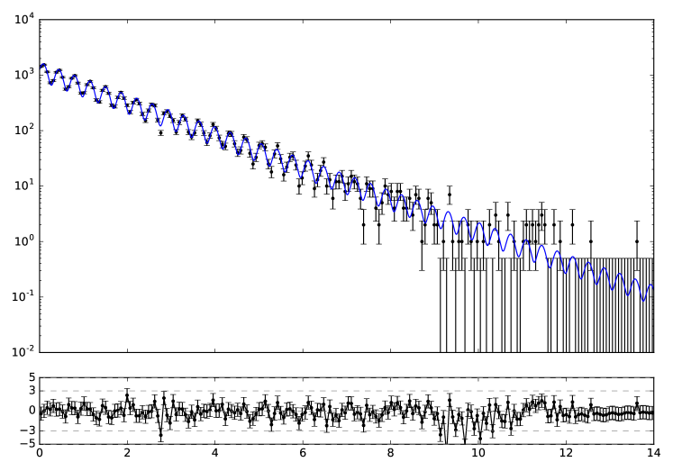
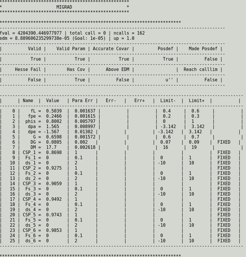
A method plotcat(Cat) creates a plot (via matplotlib) of the result in a given bin including the pulls, as shown in Fig. 2. The fit result for the case when only the P wave contributes to the final state is shown in Fig. 3. The computation times as tested on different devices are summarized in Tab. 2.

Figure 2: Plot of the fit result of Example 2: Decay time distribution in the fourth $KK$ mass bin, and flavour $B^{0}_{s}$.

Figure 3: Fit result of Example 2 for the case of a P wave contribution only: (a) MIGRAD output, (b) HESSE output, (c) parameter correlation matrix.

ParamBox also includes a method that can launch a scan of the parameter space using MultiNest ,

manager.createMultinest("mnest_party").

This is done via pymultinest. The string passed to createMultinest is the folder in which MultiNest will store its outputs. Although pymultinest has a default value for it (“./chains”), here we force the user to set it manually, to avoid reading from an unrelated chain made on the same folder. Keyword arguments will be sent to pymultinest. In addition, a keyword argument reset = True/False can be used to restart the sampling if a scan on the same folder was done before. Then, the ParamBox class provides methods to read the MultiNest output, for example

manager.mnest_vals()

prints out the most probable value. The default priors in ParamBox are flat, thus the printed values should be close to those found by Minuit, unless one of the two algorithms has converged to a local minimum or the parameter space was undersampled. Note that convergence in MultiNest will be way slower than for Minuit (although MultiNest can offer other advantages).

Table 2: Timings of the Example 2 in different devices (see text for details).

Device	10k events	10M events
	time [s]
GeForce 980 GTX Ti	1.9	60
GeForce 1080 GTX	1.8	50
Tesla M2090	1.9

5 Example 3: Binned fit to $\Upsilon\rightarrow\mu^{+}\mu^{-}$ decays in bins of $\eta$ and $p_{T}$ and search for $A^{0}\rightarrow\mu^{+}\mu^{-}$ decay

File: psilons.p
In this example, a binned fit is performed to the $\Upsilon$ resonances, on a decay into two muons of opposite sign. The fit is performed simultaneously in bins of pseudorapidity, $\eta$, and transverse momentum, $p_{T}$. The number of bins for these two variables is left to the user, and specified in two lists:

ptbins  = range(2)
etabins = range(2).

Binning scheme for the data is set using

binning = gpuarray.to_gpu(np.float64(np.linspace(5.5e3, 15e3, 512*32)))

where .e3 and 5e3 } are the bounds on the di-muon mass (in \mevcc) and {\verb 52*32 defines a number of bins in terms of the grid used later. Data is taken from a toy-MC sample, generated from a PDF as the one used in the fit. The parameters to create the sample are specified in a dictionary corresponding in this case to the intial values of those to do the fit:

genPars = {}
for p in Params:
  genPars[p.name] = p.val
manager.generateToy(genPars).

For more information on how to generate toy-MC samples see Sect. 7. When the categories (one per bin) are defined:

Cat(cat_name, idata[1], getN = True)

the input data for each category is set as binned specifying

etN =True}.
%A search for the supersymmetric li

ht spin-1 Higgs boson $A^{0}$ is also done. The $\Upsilon$ fit parameters are fixed to those saved in arams.y . The free parameter limits are specified during the initialization of the variable Params:

Params = [
  Free(’lm’, 0.47, limits = (0., 0.9)),
  Free(’lb’, -2.0, limits = (-4, -0.1)),
  Free(’a1’, 1.26, limits = (0.5, 5.)),
  Free(’n1’, 1.28, limits = (0.5, 5.)),
  Parameter(’n2’, 1.),
  Parameter(’a2’, 200.),
  Free(’beta’, -0.001, limits = (-1.e-02, 0.)),
  Free(’scale’, 1.e-04, limits = (0, 0.005)),
  Parameter(’A1_m’, 9460.30),
  ]

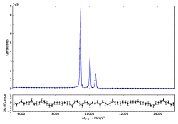
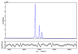
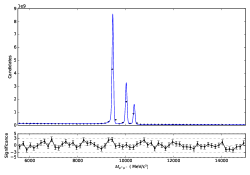
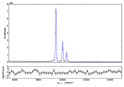
The mass model consists on a smeared Ipatia distribution, which inculdes a gaussian convolution for the multiple scattering  [10]. The MS contribution is read from ampup_paams.cpickle . As an output the mass plots for each $p_{T}$ and $\eta$ bin are shown and saved in pdf format (see Fig. 4).

(a) $\text{Bin}_{p_{T}}=0~{}~{}~{}~{}\text{Bin}_{\eta}=0$

(b) $\text{Bin}_{p_{T}}=0~{}~{}~{}~{}\text{Bin}_{\eta}=1$

(c) $\text{Bin}_{p_{T}}=1~{}~{}~{}~{}\text{Bin}_{\eta}=0$

(d) $\text{Bin}_{p_{T}}=1~{}~{}~{}~{}\text{Bin}_{\eta}=1$

Figure 4: Fits to the binned dataset of two opposite sign muons in the $\Upsilon$ range. The three peaks correspond to the three different states of the $\Upsilon$ resonance which contribute to this spectrum.

Table 3: Timings of the Example 3 in different devices (see text for details).

Device	$10^{10}$ events
	time [s]
GeForce 980 GTX Ti	$\approx$ 50
GeForce 1080 GTX	$\approx$ 50
Tesla M2090	-

6 Example 4: $\rm CL_{s}$

File: cls_beta_01.py
Limits setting and combinations of experimental results using the $\rm CL_{s}$ method (or modified frequentist approach [11, 12]) can greatly benefit from the use of GPUs, by parallelizing the computation of the toy experiments, that represent the most time-consuming part of the computation of the confidence levels. In this section a generic example is shown. This example consists on the computation of $\rm CL_{b}$,$\rm CL_{s+b}$ and $\rm CL_{s}$ in a hypothetical search experiment of a signal described by the Ipatia function [10] in the mass spectrum, on top of an exponential background. For this, a definition of the different parameters is done, such as the number of bins for the mass distribution (NBINS = 10000), as well as the the array of mass values that define the interval where the search is performed:
masslow = np.arange(5179.,5379., 200./NBINS, dtype = dtype)
DM = masslow[1] - masslow[0]
massbins = np.append(masslow, np.array(max(masslow)+DM,dtype = dtype))
mass_center = masslow +0.5*DM,
where masslow is the array of low-edges, DM its step size, massbins is defined from masslow such that the last value of the array is also incorporated, and mass_center is the corresponding array with the bin centers. After this, the Ipatia function is loaded into the GPU, and the values of its parameters are specified:
mod = SourceModule(file(os.environ["IPAPATH"] + "/cuda/psIpatia.cu","r").read())
ipa = mod.get_function("Ipatia").
In order to convert unbinned data to histograms, bins for the GPU have to be defined from mass_center:
bins_gpu = gpuarray.to_gpu(mass_center)
bins_cx = bins_gpu.astype(np.complex128)
Note that there are two sets of bins: the ones of type np.float64 are used for both the Ipatia and exponential PDF that will be used later for the background, while the bins of type np.complex128 will be necessary when convolving the Ipatia with a Gaussian function.
The array corresponding to the signal distribution is created as an empty array with the size of mass_center, filled via the Ipatia function and then convolved with a Gaussian function as follows:
ipa(bins_gpu, sigf_i_gpu, np.float64(mu),np.float64(sigma),np.float64(l), np.float64(beta), np.float64(a), np.float64(n), np.float64(a2),
np.float64(n2) , block = (1000,1,1), grid = (max(len(tmp0)/1000,1),1))
SM = GaussSmear1(bins_cx,sigma0)
sigf_gpu = SM.Smear(sigf_i_gpu).
As for the background distribution, an array of the same length as sigf_gpu is filled following an exponential function, $\exp(-\rm kx)$, where k is set to be -0.001 and x is the mass value. Both signal and background distributions are normalized to 1:
sigpdf_gpu = sigf_gpu/np.sum((sigf_gpu).get())
bkgpdf_gpu = bkgf_gpu/np.sum((bkgf_gpu).get()).
From these PDFs, the data that will be used for the $\rm CL_{s}$ computation is generated, setting the number of expected events for both signal (ns) and background (nb).
def HistoPdf(ns =5000, nb = Nb): return np.float64(ns) * sigpdf_gpu + np.float64(nb)*bkgpdf_gpu
fake_data = gpuarray.to_gpu(np.uint32(tmp0))
generateBinned(fake_data, HistoPdf(ns = 70)).
Finally, the confidence levels and $\rm CL_{s}$ are calculated as a function of the signal strength or number of signal events. The number of toy experiments used can be modified, and for the sake of this example is set to the default value (10000 toys), good enough to get proper precision.
CL = CLcalculator()
CL.setData(fake_data)
CL.setExpected(HistoPdf)
CL.CLs(70, toys = 10000)

Table 4: Timings of the example 4 in different devices (See text for details).

Device	time $(s)$ per event
GeForce 980 GTX Ti	10.6
GeForce 1080 GTX	12.8
Tesla M2090	41.7

7 Example 5: Generating ToyMC

GPU devices can also be used to generate toyMC. For binned PDFs, it can be done via generateBinned as shown in the examples of $\textrm{CL}_{\textrm{s}}$ and $A^{0}\to\mu\mu$. Generating unbinned datasets require somewhat more gymnastics, but can also be done without too much effort, as we will discuss now. CUDA random generators are imported via curand.h and curand_kernel.h. It must be noted that the latter cannot be included inside an extern "C", which is what SourceModule automatically wraps the code in. Thus, we have to invoke SourceModule (or cuRead) with the keyword argument no_extern_c = True. Then we should place extern "C" manually inside our CUDA file, after the inclusion of the generators and before the function definitions.

Once this is done, one can proceed and use curand_init, curand_uniform etc to generate random numbers, and create toyMC. The generation can be done for instance by using the accept-reject method.

An example of this is shown in file:

examples/toyMC/fitphis.py

The above is a modified version of the example presented in Sect. 4, where we generate a random dataset for one of the categories of the fit, and plot it on top of the ${\rm PDF}$. The example can easily be expanded to generate datasets for all categories, as well as to include Poissonian random fluctuations on the generated number of events. For this we suggest generating Nevts in the Python class with scipy.random.poisson or scipy.random.normal, and modifying the grid and block sizes accordingly. The timing of the example measured in different setups is shown in Table 5.

Table 5: Timings of Example 5 in different devices (see text for details).

Device	133 725 events	6 769 840 events
	time [s]
GeForce 980 GTX Ti	0.11	0.34
GeForce 1080 GTX	0.13	0.30
Tesla M2090	-	-

Combining with Symbolic programing

When dealing with complicated models, symbolic programing can be very useful. In Python this can be done through sympy. In that case, being able to convert a symbolic expression to a CUDA piece of code greatly simplifies the development of GPU fits. For instance, the angular PDFs and the corresponding integrals in the $B^{0}_{s}\to{{J\mskip-3.0mu/\mskip-2.0mu\psi\mskip 2.0mu}}K^{+}K^{-}$ example were obtained this way. Another example of this is

examples/urania/faddeeva.py,

where the limit expression of Faddeva’s functions at large $t/\sigma$ are obtained, and converted to __device__ CUDA functions.

A more complicated (and, sadly, cryptic) example can be found at:

examples/urania/JpsiPhiTimeFit_forRooFit.py.

where the $B^{0}_{s}\to{{J\mskip-3.0mu/\mskip-2.0mu\psi\mskip 2.0mu}}\phi$ time-dependent angular distribution is printed to LaTex and .pdf files as well as to a RooFit fitting class. By enabling the flag USE_MATHEMATICA one can get the integral over time from Mathematica instead of sympy, as the latter is sometimes worse at simplification. The Python list Spins lists the spins of the $hh$ resonances one wants to generate, i.e, [1] for P–wave, [0,1] for S–wave and P–wave, [0,1,2] to also include D–wave, etc… One can similarly make an script to create CUDA code. The following examples:

examples/urania/JpsiPhiTimeFit_forCuda.py
examples/urania/JpsiPhiTimeFit_forCuda_Bbar.py

create CUDA files with the function, the integrals and the derivatives.

8 FAQ

• Can I add prints/std::outs to my cuda stuff?: Yes, #include $<stdio.h>$ and you could use printf at least on the __global__ functions. You can also pass a gpuarray to your program and store on it intermediate numbers that you want to check, it will be visible from Python.

Appendix A ParamBox class

The class ParamBox is defined in ModelBricks.py. To initizalize an instance, one needs to provide a list of fit parameters and (optionally) a list of categories (class Cat). The following methods are contained in ParamBox:

• freeThese(pars): Frees each parameter in the provided list

• lock_to_init(pars): Fixes each parameter in the provided list

• createFit(): Initializes a Minuit fit providing it with a list of parameters

• createMultinest(savedir,reset = False,**kwargs): Runs a Multinest scan with the fit result as an input and saves the output in a directory

• readMultinest(savedir): Reads an existing Multinest output and prints its result

• fitSummary(): Creates an instance of the class FitSummary (defined in the same file), which contains the fit result information, such as the parameter values, parameter errors, fit matrix etc.

• saveFitSummary(name): Saves the fit result information into a cPickle file with the name provided

Appendix B Parameter class

The class Parameter, defined in ModelBricks.py, handles the information of each parameter in the fit. It is initialized with a name and, optionally, an initial value, range limits, a step size, a flag indicating whether it is constant (default), and a type. The following methods are contained in Parameter:

• setVal(var): Sets the initial value

• autoStepSize(): Sets the step size to one tenth of the parameter range (determined by the limits)

• setLimits(m,M, constant = False): Sets the lower and upper limits and, optionally, changes the constant flag

• getSettings(): Returns a dictionary with the available information of the parameter (value, limits, error and whether it is constant)

The class Free is completely equivalent to Parameter but with the option constant=False set by default.

Appendix C Cat class

The information in each category of a simultaneous fit is handled by the class Cat, defined in ModelBricks.py. An instance of this class is initialized with a name for the category. Additionally, a dataset (GPU array, numpy ndarray, list, cPickle file or string) can be provided. If getN=True is added as extra argument, the class will determine the size of the given sample. Alternatively, the user can specify the size by setting N to the desired value in the arguments.

When an instance of the class Cat is initialized, the following two methods are called (if possible):

• setData(ary, getN = False): Creates a GPU array to store the provided dataset

• bookProbs(N): Books a GPU array with the size of the data for the likelihood probability values at each point

Appendix D Hardware

Here, we give some hardware specifications for the graphics cards used to test the examples in this documentation.

Table 6: Specifications of the graphics cards used for testing the examples.

	GeForce 980 GTX Ti	GeForce 1080 GTX	Tesla M2090
CUDA cores	2816	2560	512
Single precision (GFLOPS)	5632	8228 (8873)	1331.2
Double precision (GFLOPS)	176	257 (277)	665.6
Memory size (GiB)	6.1	8	6.1
Memory Bandwidth (GB/s)	336.5	320	177.6

References

- [1] A. Klöckner, N. Pinto, Y. Lee, B. Catanzaro, P. Ivanov and A. Fasih, Pycuda and pyopencl: A scripting-based approach to gpu run-time code generation, Parallel Comput. 38 (Mar., 2012) 157–174.
- [2] “Iminuit - interactive ipython friendly minimizer based on seal minuit.” https://github.com/iminuit/iminuit, 2017.
- [3] F. James and M. Winkler. http://www.cern.ch/minuit, May, 2004.
- [4] Buchner, J., Georgakakis, A., Nandra, K., Hsu, L., Rangel, C., Brightman, M. et al., X-ray spectral modelling of the agn obscuring region in the cdfs: Bayesian model selection and catalogue⋆⋆⋆, A&A 564 (2014) A125.
- [5] “Anaconda.” https://docs.continuum.io/anaconda/, 2017.
- [6] “reikna.” http://reikna.publicfields.net/en/latest/, 2017.
- [7] F. Feroz, M. P. Hobson and M. Bridges, Multinest: an efficient and robust bayesian inference tool for cosmology and particle physics, Monthly Notices of the Royal Astronomical Society 398 (2009) 1601.
- [8] LHCb collaboration, R. et al.. Aaij, Precision measurement of violation in decays, Phys. Rev. Lett. 114 (2015) 041801.
- [9] D. J. Lange, The EvtGen particle decay simulation package, Nucl. Instrum. Meth. A462 (2001) 152–155.
- [10] D. Martínez Santos and F. Dupertuis, Mass distributions marginalized over per-event errors, Nucl. Instrum. Meth. A764 (2014) 150–155, [1312.5000].
- [11] T. Junk, Confidence level computation for combining searches with small statistics, Nucl. Instrum. Meth. A434 (1999) 435–443, [hep-ex/9902006].
- [12] A. L. Read, Presentation of search results: The CL(s) technique, J. Phys. G28 (2002) 2693–2704.