The Fierz convergence criterion: a controlled approach to strongly-interacting systems with small embedded clusters

Abstract

We present an embedded-cluster method, based on the TRILEX formalism. It turns the Fierz ambiguity, inherent to approaches based on a bosonic decoupling of local fermionic interactions, into a convergence criterion. It is based on the approximation of the three-leg vertex by a coarse-grained vertex computed by solving a self-consistently determined multi-site effective impurity model. The computed self-energies are, by construction, continuous functions of momentum. We show that, in three interaction and doping regimes of parameters of the two-dimensional Hubbard model, self-energies obtained with clusters of size four only are very close to numerically exact benchmark results. We show that the Fierz parameter, which parametrizes the freedom in the Hubbard-Stratonovich decoupling, can be used as a quality control parameter. By contrast, the $GW$+extended dynamical mean field theory approximation with four cluster sites is shown to yield good results only in the weak-coupling regime and for a particular decoupling. Finally, we show that the vertex has spatially nonlocal components only at low Matsubara frequencies.

Two major approaches have been put forth to fathom the nature of high-temperature superconductivity. Spin fluctuation theoryChubukov et al. (2002); Onufrieva and Pfeuty (2009); Metlitski and Sachdev (2010); Efetov et al. (2013); Onufrieva and Pfeuty (2012); Scalapino (2012); Wang and Chubukov (2014); Wang et al. (2016), inspired by the early experiments on cuprate compounds, is based on the introduction of phenomenological bosonic fluctuations coupled to the electrons. It belongs to a larger class of methods, including the fluctuation-exchange (FLEX)Bickers and Scalapino (1989) and $GW$ approximationsHedin (1965, 1999), or the Eliashberg theory of superconductivityEliashberg (1960). In the Hubbard model, these methods can formally be obtained by decoupling the electronic interactions with Hubbard-Stratonovich (HS) bosons carrying charge, spin or pairing fluctuations. They are particularly well suited for describing the system’s long-range modes. However, they suffer from two main drawbacks: without an analog of Migdal’s theorem for spin fluctuations, they are quantitatively uncontrolled; worse, the results depend on the precise form of the bosonic fluctuations used to decouple the interaction term, an issue referred to as the “Fierz ambiguity”Jaeckel and Wetterich (2003); Baier et al. (2004); Bartosch et al. (2009); Borejsza and Dupuis (2003, 2004); Dupuis (2002).

A second class of methods, following AndersonAnderson (1987), puts primary emphasis on the fact that the undoped compounds are Mott insulators, where local physics plays a central role. Approaches like dynamical mean field theory (DMFT)Georges et al. (1996) and its cluster extensionsHettler et al. (1998, 1999); Lichtenstein and Katsnelson (2000); Kotliar et al. (2001); Maier et al. (2005a), which self-consistently map the lattice problem onto an effective problem describing a cluster of interacting atoms embedded in a noninteracting host, are tools of choice to examine Anderson’s idea. Cluster DMFT has indeed been shown to give a consistent qualitative picture of cuprate physics, including pseudogap and superconducting phasesKyung et al. (2009); Sordi et al. (2012a); Civelli et al. (2008); Ferrero et al. (2010); Gull et al. (2013); Macridin et al. (2004); Maier et al. (2004, 2005b, 2006); Gull et al. (2010); Yang et al. (2011a); Macridin and Jarrell (2008); Macridin et al. (2006); Jarrell et al. (2001); Parcollet et al. (2004); Werner et al. (2009); Biroli et al. (2004); Bergeron et al. (2011); Kyung et al. (2004, 2006); Okamoto et al. (2010); Sordi et al. (2010, 2012b); Civelli et al. (2005); Ferrero et al. (2008, 2009); Gull et al. (2009); Chen et al. (2015, 2017). Compared to fluctuation theories, it a priori comes with a control parameter, the size $N_{c}$ of the embedded cluster. However, this is of limited practical use, since the convergence with $N_{c}$ is nonmonotonic for small $N_{c}$Maier et al. (2005b), requiring large $N_{c}$’s, which cannot be reached in interesting physical regimes due to the Monte-Carlo negative sign problem. Thus, converged cluster DMFT results can only be obtained at high temperaturesLeBlanc et al. (2015). There, detailed studiesGunnarsson et al. (2015, ); Wu et al. point to the importance of (possibly long-ranged) spin fluctuations, calling for a unification of both classes of approaches. First steps in this direction have been accomplished by diagrammatic extensions of DMFTRohringer et al. ; Biermann et al. (2003); Sun and Kotliar (2002, 2004); Ayral et al. (2012, 2013); Biermann (2014); Ayral et al. ; Rubtsov et al. (2008, 2012); van Loon et al. (2014); Stepanov et al. (2016); Toschi et al. (2007); Katanin et al. (2009); Schäfer et al. (2015); Valli et al. (2015); Li et al. (2016); Rohringer and Toschi (2016); Ayral and Parcollet (2016a); Hafermann et al. (2008); Slezak et al. (2009); Yang et al. (2011b), and by the single-site TRILEX formalismAyral and Parcollet (2015, 2016b), which interpolates between long-range and Mott physics, and describes aspects of pseudogap physics and the $d$-wave superconducting domeVučičević et al. .

In this Letter, we turn the Fierz ambiguity into a convergence criterion in the cluster extension of TRILEX. Like fluctuation approaches, cluster TRILEX is based on the introduction of bosonic degrees of freedom. Like cluster DMFT, it maps the corresponding electron-boson problem onto a cluster impurity problem. The latter is solved for its three-leg vertex, which is used as a cluster vertex correction to the self-energies. This approach improves on fluctuation approaches by endowing them with a control parameter, thus curing the absence of a Migdal theorem. In some parameter regimes, it can solve the cluster DMFT large-$N_{c}$ stalemate by instead requiring minimal sensitivity to the Fierz parameter as a convergence criterion of the solution.

To illustrate the method, we focus on the two-dimensional Hubbard model, the simplest model to describe high-temperature superconductors. It is defined by the Hamiltonian:

$$H=\sum_{ij\sigma}t_{ij}c_{i\sigma}^{\dagger}c_{j\sigma}+U\sum_{i}n_{i\uparrow}n_{i\downarrow}$$ (1)

where $c_{i\sigma}^{\dagger}$ ($c_{i\sigma}$) creates (annihilates) an electron of spin $\sigma$ at Bravais site $\mathbf{r}_{i}$, $t_{ij}$ is the hopping matrix (with [next-]nearest-neighbor hopping parametrized by $t$ [$t^{\prime}$]), and $U$ the local electronic repulsion. We set $t=-0.25$ and use $D\equiv 4|t|$ as the energy unit.

The first step of the TRILEX method consists in decoupling the interaction term with HS fields. There are several possible such decouplings, a fact called the Fierz ambiguity. Here, we choose to express the interaction in the charge and longitudinal spin channel (“Ising decoupling”), i.e, up to a density term:

$$Un_{i\uparrow}n_{i\downarrow}=\frac{1}{2}U^{\mathrm{ch}}n_{i}n_{i}+\frac{1}{2}U^{\mathrm{sp}}s_{i}^{z}s_{i}^{z}$$ (2)

with $n\equiv n_{\uparrow}+n_{\downarrow}$ and $s^{z}\equiv n_{\uparrow}-n_{\downarrow}$.This holds provided $U^{\mathrm{ch}}-U^{\mathrm{sp}}=U$, or equivalently

$$U^{\mathrm{ch}} =\alpha U,\;\;U^{\mathrm{sp}}=(\alpha-1)U$$ (3)

The “Fierz parameter” $\alpha$ materializes the freedom in choosing the charge-to-spin fluctuation ratio. The right-hand side of Eq. (11) is decoupled with a charge and a spin boson, resulting in an electron-boson coupling problemAyral and Parcollet (2015, 2016b). Its fermionic and bosonic interacting Green’s functions are given by Dyson equations:

$$G(\mathbf{k},i\omega) =\frac{1}{i\omega+\mu-\varepsilon(\mathbf{k})-\Sigma(\mathbf{k},i\omega)}$$ (4a)

$$W^{\eta}(\mathbf{q},i\Omega) =\frac{U^{\eta}}{1-U^{\eta}P^{\eta}(\mathbf{q},i\Omega)}$$ (4b)

$\varepsilon(\mathbf{k})$ is the Fourier transform of $t_{ij}$ ($\varepsilon(\mathbf{k})=2t\left(\cos(k_{x})+\cos(k_{y})\right)+4t^{\prime}\cos(k_{x})\cos(k_{y})$), $\mu$ the chemical potential, $\eta=\mathrm{ch},\mathrm{sp}$, and $i\omega$ [resp. $i\Omega$] denote fermionic [resp. bosonic] Matsubara frequencies. The self-energy $\Sigma(\mathbf{k},i\omega)$ and polarization $P^{\eta}(\mathbf{q},i\Omega)$ are given by the exact Hedin expressions:

$$\Sigma(\mathbf{k},i\omega)=$$ (5a)

$$\;\;-\sum_{\eta}\sum_{\mathbf{q},i\Omega}G(\mathbf{k}+\mathbf{q},i\omega+i\Omega)W^{\eta}(\mathbf{q},i\Omega)\Lambda_{\mathbf{k}\mathbf{q}}^{\eta}(i\omega,i\Omega)$$

$$P^{\eta}(\mathbf{q},i\Omega)=$$ (5b)

$$\;\;2\sum_{\mathbf{k},i\omega}G(\mathbf{k}+\mathbf{q},i\omega+i\Omega)G(\mathbf{k},i\omega)\Lambda_{\mathbf{k}\mathbf{q}}^{\eta}(i\omega,i\Omega)$$

$\Lambda_{\mathbf{k}\mathbf{q}}^{\eta}(i\omega,i\Omega)$ is the interacting electron-boson vertex. TRILEX approximates it with a vertex computed from a self-consistent impurity model. In previous worksAyral and Parcollet (2015, 2016b), this impurity model contained a single site.

There are several ways to extend the TRILEX method to cluster impurity problems, like in DMFT. Here, we consider the analog of the dynamical cluster approximation (DCAHettler et al. (1998, 1999); Maier et al. (2005a)), and use periodic clusters so as not to break the lattice translational symmetry, at the price of discontinuities in the momentum dependence of the vertex function. Other cluster variants such as a real-space version, inspired from cellular DMFTLichtenstein and Katsnelson (2000); Kotliar et al. (2001), are also possible, but break translation invariance and require arbitrary reperiodization procedures.

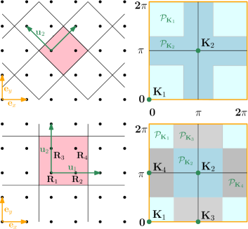
Figure 1: Cluster geometry: real (left) and reciprocal (right) space, for $N_{c}=2$ (top) and $N_{c}=4$ (bottom). $\mathbf{e}_{x}$ and $\mathbf{e}_{y}$ ($\mathbf{u}_{1}$ and $\mathbf{u}_{2}$) are the unit vectors of the Bravais (super)lattice. The colored patches $\mathcal{P}_{\mathbf{K}_{i}}$ are of equal area

We straighforwardly generalize the single-site impurity model of TRILEX to a cluster impurity model defined by the action:

$$S_{\mathrm{imp}}\equiv\iint_{\tau\tau^{\prime}}\sum_{ij\sigma}c_{i\sigma\tau}^{*}\left\{-\left[\mathcal{G}^{-1}\right]_{ij}(\tau-\tau^{\prime})\right\}c_{j\sigma\tau^{\prime}}$$ (6)

$$+\frac{1}{2}\iint_{\tau\tau^{\prime}}\sum_{ij}\left\{n_{i\tau}\mathcal{U}_{ij}^{\mathrm{ch}}(\tau-\tau^{\prime})n_{j\tau^{\prime}}+s_{i\tau}^{z}\mathcal{U}_{ij}^{\mathrm{sp}}(\tau-\tau^{\prime})s_{j\tau^{\prime}}^{z}\right\}$$

The latin indices $i,j=1\dots N_{c}$ stand for the cluster positions $\mathbf{R}_{i}$, $\mathbf{R}_{j}$ (shown in Fig. 1 along with the cluster momenta $\{\mathbf{K}_{i}\}_{i=1\dots N_{c}}$). $c_{i\sigma\tau}^{*}$ and $c_{i\sigma\tau}$ are conjugate Grassmann fields, $\tau$ denotes imaginary time. Since we have introduced a charge and a spin bosonic mode, the impurity action contains interactions in both channels ($\mathcal{U}^{\mathrm{ch}}(\tau)$ and $\mathcal{U}^{\mathrm{sp}}(\tau)$). They are a priori retarded due to the nonlocal character of $P^{\eta}(\mathbf{q},i\Omega)$.

This cluster impurity model is used to compute the cluster impurity vertex $\Lambda_{\mathrm{imp}}^{\eta}(\mathbf{K},\mathbf{Q};i\omega,i\Omega)$ with a continuous-time quantum Monte-Carlo algorithm with a hybridization [resp. interaction] expansion for $N_{c}=1$ [resp. $N_{c}=2,4$] (as described in Suppl. Mat. B.3). Next, in the spirit of DCA, we want to use $\Lambda_{\mathrm{imp}}^{\eta}(\mathbf{K},\mathbf{Q};i\omega,i\Omega)$ to approximate the momentum dependence of the lattice vertex $\Lambda_{\mathbf{k}\mathbf{q}}^{\eta}(i\omega,i\Omega)$ by a coarse-graining procedure. We recall that DCA consists in coarse-graining the cluster self-energy as $\Sigma(\mathbf{k},i\omega)\approx\sum_{\mathbf{K}}\theta_{\mathbf{K}}(\mathbf{k})\Sigma_{\mathrm{imp}}(\mathbf{K},i\omega)$, where $\Sigma_{\mathrm{imp}}(\mathbf{K},i\omega)$ is the cluster impurity self-energy, and $\theta_{\mathbf{K}}(\mathbf{k})=1$ if $\mathbf{k}$ belongs to Brillouin-zone patch $\mathcal{P}_{\mathbf{K}}$, and vanishes otherwise. For the vertex function, the passage from $\Lambda_{\mathrm{imp}}^{\eta}(\mathbf{K},\mathbf{Q};i\omega,i\Omega)$ to an approximate lattice vertex $\Lambda_{\mathbf{k},\mathbf{q}}^{\eta}(i\omega,i\Omega)$ is not as straightforward. There are several possible coarse-grainings for the vertex that reduce to single-site TRILEX for $N_{c}=1$ and are exact in the $N_{c}=\infty$ limit, e.g.

$$\Lambda_{\mathbf{k}\mathbf{q}}^{\eta}(i\omega,i\Omega) \approx\sum_{\mathbf{K},\mathbf{Q}}\theta_{\mathbf{K}+\mathbf{Q}}(\mathbf{k}+\mathbf{q})\theta_{\mathbf{Q}}(\mathbf{q})\Lambda_{\mathrm{imp}}^{\eta}(\mathbf{K},\mathbf{Q};i\omega,i\Omega)$$ (7a)

$$\Lambda_{\mathbf{k}\mathbf{q}}^{\eta}(i\omega,i\Omega) \approx\sum_{\mathbf{K},\mathbf{Q}}\theta_{\mathbf{K}}(\mathbf{k})\theta_{\mathbf{K}+\mathbf{Q}}(\mathbf{k}+\mathbf{q})\Lambda_{\mathrm{imp}}^{\eta}(\mathbf{K},\mathbf{Q};i\omega,i\Omega)$$ (7b)

We use a different coarse-graining for $\Sigma$ and for $P$: we substitute (7a) in (5a) [resp. (7b) in (5b)] to compute $\Sigma(\mathbf{k},i\omega)$ [resp. $P^{\eta}(\mathbf{q},i\Omega)$], whence:

$$\Sigma(\mathbf{k},i\omega)=$$ (8a)

$$-\sum_{\eta,\mathbf{K},\mathbf{Q}}\sum_{\mathbf{q},i\Omega}G_{\mathbf{k}+\mathbf{q}}^{\mathbf{K}+\mathbf{Q}}(i\omega+i\Omega)W_{\mathbf{q}}^{\eta,\mathbf{Q}}(i\Omega)\Lambda_{\mathrm{imp}}^{\eta}(\mathbf{K},\mathbf{Q};i\omega,i\Omega)$$

$$P^{\eta}(\mathbf{q},i\Omega)=$$ (8b)

$$2\sum_{\mathbf{K},\mathbf{Q}}\sum_{\mathbf{k},i\omega}G_{\mathbf{k}+\mathbf{q}}^{\mathbf{K}+\mathbf{Q}}(i\omega+i\Omega)G_{\mathbf{k}}^{\mathbf{K}}(i\omega)\Lambda_{\mathrm{imp}}^{\eta}(\mathbf{K},\mathbf{Q};i\omega,i\Omega)$$

with $X_{\mathbf{k}}^{\mathbf{K}}(i\omega)\equiv\theta_{\mathbf{K}}(\mathbf{k})X(\mathbf{k},i\omega)$ (for $X=G$ and $W$). As convolutions of continuous functions of $\mathbf{k}$ ($G$ and $W$) with a piecewise-constant function ($\Lambda$), $\Sigma$ and $P$ are continuous in $\mathbf{k}$ by construction.

Finally, the cluster dynamical mean fields $\mathcal{G}_{ij}(\tau)$ and $\mathcal{U}_{ij}^{\eta}(\tau)$ are determined by imposing the following self-consistency conditions:

$$G_{\mathrm{imp}}(\mathbf{K},i\omega)[\mathcal{G},\mathcal{U}] =G_{\mathbf{K}}(i\omega)$$ (9a)

$$W_{\mathrm{imp}}^{\eta}(\mathbf{Q},i\Omega)[\mathcal{G},\mathcal{U}] =W_{\mathbf{Q}}^{\eta}(i\Omega)$$ (9b)

The left-hand sides are computed by solving the impurity model. The right-hand sides are the patch-averaged lattice Green’s functions:

$$G_{\mathbf{K}}(i\omega) \equiv\sum_{\mathbf{k}\in\mathcal{P}_{\mathbf{K}}}G(\mathbf{k},i\omega)$$ (10a)

$$W_{\mathbf{Q}}^{\eta}(i\Omega) \equiv\sum_{\mathbf{q}\in\mathcal{P}_{\mathbf{Q}}}W^{\eta}(\mathbf{q},i\Omega)$$ (10b)

The determination of $\mathcal{G}$ and $\mathcal{U}^{\eta}$ satisfying Eq. (9a-9b) is done by forward recursion (see Suppl. Mat. B.2).

We have implemented this method and studied it in three physically distinct parameter regimes: (A) Weak-coupling regime ($U/D=0.5$, $\delta=0\%$, $\beta D=16$, $t^{\prime}=0$) at half-filling, (B) Intermediate-coupling regime ($U/D=1$, $\delta=20\%$, $\beta D=16$, $t^{\prime}=0$) at large doping, (C) Strong-coupling regime ($U/D=1.4$, $\delta=4\%$, $\beta D=8$, $t^{\prime}/t=-0.3$) at small doping (the Mott transition occurs at $U_{c}/D\approx 1.5$ within plaquette cellular DMFTPark et al. (2008)). We solve at point A, B, C for different values of $\alpha$.

In the absence of any approximation, every HS decoupling, hence every value of $\alpha$, yields the same result: the exact solution does not depend on $\alpha$. The cluster TRILEX approximation a priori breaks this property, but as $N_{c}$ increases, we expect the $\alpha$-dependence to become weaker. We propose to use the weak $\alpha$-dependence for a given $N_{c}$, i.e. the existence of a plateau for at least a range $\alpha$, as a (Fierz) convergence criterion. Whether this criterion is sufficient to establish convergence is an assumption, which we test here using exact benchmarks for points A, B and C. Indeed, at these temperatures, interactions and dopings, determinant quantum Monte Carlo (QMC) and/or DCA can be converged and give a numerically exact solution of the Hubbard model, albeit at a significant numerical cost.

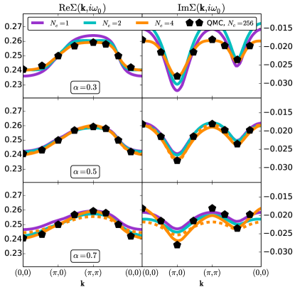
Figure 2: Point A ($U/D=0.5$, $\delta=0\%$, $\beta D=16$, $t^{\prime}=0$). $\mathrm{Re}\Sigma(\mathbf{k},i\omega_{0})$ (left) and $\mathrm{Im}\Sigma(\mathbf{k},i\omega_{0})$ (right) for $N_{c}=1,2,4$ for various values of $\alpha$ (from top to bottom), along the path $(0,0)-(\pi,0)-(\pi,\pi)-(0,0)$. Solid lines: TRILEX. Dashed lines: $GW$+EDMFT ($N_{c}=4$). Pentagons: determinant QMC (only a subset of $\mathbf{K}$ points is shown for better visibility).

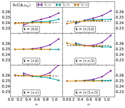
Figure 3: Dependence of $\mathrm{Re}\Sigma(\mathbf{k},i\omega_{0})$ on $\alpha$ for different momenta (Point A: $U/D=0.5$, $\delta=0\%$, $\beta D=16$, $t^{\prime}=0$). Black dashed lines: QMC.

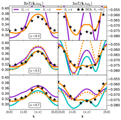
Figure 4: $\Sigma(\mathbf{k},i\omega_{0})$ at point B ($U/D=1$, $\delta=20\%$, $\beta D=16$, $t^{\prime}=0$). Same conventions as Fig. S.1. Dashed lines: $GW$+EDMFT. Stars: DCA from Ref. LeBlanc et al., 2015.

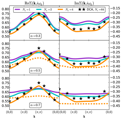
Figure 5: $\Sigma(\mathbf{k},i\omega_{0})$ at point C ($U/D=1.4$, $\delta=4\%$, $\beta D=8$, $t^{\prime}/t=-0.3$). Same conventions as Fig. S.1. Dashed lines: $GW$+EDMFT. Stars: DCA.

We start with point A. In Fig. S.1, we show the self-energy $\Sigma(\mathbf{k},i\omega_{0})$ for cluster sizes of $N_{c}=1$ (single-site), $2$ (dimer) and 4 (plaquette) and for three different values of $\alpha$. As expected, the dependence on $\alpha$ becomes weaker as $N_{c}$ increases. At $N_{c}=4$, the self-energy is almost independent on $\alpha$. The $\alpha$-dependence for $N_{c}=1,2,4$ is further illustrated in Fig. 3: the $N_{c}=4$ results show an extended plateau which is narrower or nonexistent for $N_{c}=1,2$.

The benchmarks, using numerically exact determinant QMCBlankenbecler et al. (1981) computed with $N_{c}=16\times 16$ sites, are also presented on both Fig. S.1 and Fig. 3. We observe a very good agreement between $N_{c}=4$ and the benchmark data, both for the real and imaginary parts of the self-energy, which validates the Fierz criterion in this regime. We also observe that for $\alpha=0.5$, the results are in agreement with the converged values regardless of $N_{c}$. This can be understood by noticing that $\alpha=0.5$ corresponds to the values of $U^{\eta}$ used in the random phase approximation (RPA), which is correct to second order in $U$.

Moreover, we compare our results with the self-energy obtained by the $GW$+EDMFTBiermann et al. (2003); Sun and Kotliar (2002, 2004); Ayral et al. (2012, 2013); Biermann (2014); Ayral et al. method for $N_{c}=4$. $GW$+EDMFT can be regarded as a simplification of TRILEX where the vertex corrections are neglected in the nonlocal self-energy contribution. This explains why the $GW$+EDMFT results are, independently of $\alpha$, quite close to the single-site TRILEX results: the vertex frequency and momentum dependences are weak in the low-$U$ limit. Besides, they are different from the cluster TRILEX results and from the exact solution, except for the RPA value of $\alpha$ ($\alpha=0.5$) where both methods give results close to the exact solution.

At point B (Fig. S.2), the agreement between the benchmarks and the real and imaginary parts of the self-energy, for all values of $\alpha$ (with more important deviations for $\alpha=0.3$), is very good for $N_{c}=4$. Contrary to the weak-coupling limit, no value of $\alpha$ in the single-site case matches the exact solution. This points to the importance of nonlocal corrections to the three-leg vertex. This observation is further corroborated by looking at the $GW$+EDMFT curve. There, the agreement with the exact result is quite poor, while being similar to the single-site result, like in the weak-coupling limit (for $\alpha=0.3$, a spin instability precludes convergence of $GW$+EDMFT and cluster TRILEX for $N_{c}=2$). This discrepancy shows that as interactions are increased, the vertex frequency and momentum dependence play a more and more important role in the nonlocal self-energy, as we will discuss below. These conclusions are also valid for local observables (see Suppl. Mat. C.3).

At the strong-coupling point C (Fig. S.3), similarly to the previous regimes, the $N_{c}=4$ self-energy is almost independent of $\alpha$, and in good agreement with the converged (DCA) solution (especially for its real part). $GW$+EDMFT at $N_{c}=4$ is quite far from the exact result, as can be expected from the previous discussion.

Finally, we analyze the momentum and frequency dependence of the vertex, illustrated in Fig. 6. At low Matsubara frequencies, the vertex acquires a momentum dependence (especially in the charge channel), while it is essentially local at high frequencies. In other words, the largest deviations to locality occur at small frequencies only (see also Suppl. Mat. C.4). The nonlocal components are smaller or much smaller than the local component, especially for large Matsubara frequencies. This gives an a posteriori explanation of the qualitatively good results of the single-site TRILEX approximation. More importantly, the fact that the momentum dependence is confined to low frequencies suggests optimizations for the vertex parametrization and computation.

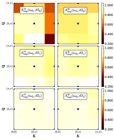
Figure 6: Point B ($U/D=1$, $\delta=20\%$, $\beta D=16$, $t^{\prime}=0$), $\alpha=0.5$. Impurity vertex $\Lambda_{\mathrm{imp}}^{\eta}(\mathbf{K},\mathbf{Q};i\omega_{0},i\Omega)$ at $\mathbf{K},\mathbf{Q}\in[(0,0),(0,\pi),(\pi,\pi)]^{2}$ (the value is color-coded in the square area surrounding each blue point) in the charge (left) and spin (right) channels, for increasing bosonic Matsubara frequency (from top to bottom).

In conclusion, we have presented a first implementation of the cluster extension of the TRILEX method. For a broad interaction and doping range of the two-dimensional Hubbard model, we obtain, for an embedded cluster with only four impurity sites, continuous self-energies in close agreement with the exact result obtained with comparatively expensive large-cluster lattice QMC and DCA calculations.

Cluster TRILEX is based on the computation and momentum coarse-graining of the three-leg vertex function: it thus comes at a cost lower than cluster methods based on four-leg verticesHafermann et al. (2008); Slezak et al. (2009), but it a priori suffers from the Fierz ambiguity. We have shown that this ambiguity can be turned into a practical advantage in two ways: First and foremost, we have shown that proximity to the exact solution coincides with stability with respect to the Fierz parameter $\alpha$ . With this necessary condition, one can assess, at a given (possibly small) cluster size, the accuracy of the solution. Second, in some regimes, there exists a value of $\alpha$ for which accurate results can be reached for smaller cluster sizes. By allowing to extract more information from smaller embedded TRILEX clusters, the Fierz convergence criterion paves the way to a controlled exploration of low-temperature phases such as superconducting phases, where cluster DMFT cannot be converged in practice.

This Supplemental Material is organized as follows: in Section A, we show results corresponding to another decoupling than the Ising decoupling used in the main text, namely the Heisenberg decoupling. In Section B, we give the technical details relevant to the implementation of the cluster TRILEX method. Finally, in Section C, we give supplementary data to complement the figures and discussion of the main text.

Supplemental Material A Self-energy in the Heisenberg decoupling: $\alpha$ and $N_{c}$ dependence and comparison to exact benchmarks

Figure S.1: Point A in the Heisenberg decoupling ($U/D=0.5$, $\delta=0\%$, $\beta D=16$). $\mathrm{Re}\Sigma(\mathbf{k},i\omega_{0})$ (left column) and $\mathrm{Im}\Sigma(\mathbf{k},i\omega_{0})$ (right column) for $N_{c}=1,2,4$ for various values of the Fierz parameter $\alpha$ (from top to bottom), along the path $(0,0)-(\pi,0)-(\pi,\pi)-(0,0)$. Solid lines: TRILEX. Dashed lines: $GW$+EDMFT ($N_{c}=4$). Pentagons: determinant QMC ($N_{c}=256$; only a small subset of $\mathbf{K}$ points is shown for a better visibility).

Figure S.2: Point B in the Heisenberg decoupling ($U/D=1$, $\delta=20\%$, $\beta D=16$). Same conventions as Fig. S.1. Stars: DCA from Ref. LeBlanc et al., 2015, $N_{c}=50$.

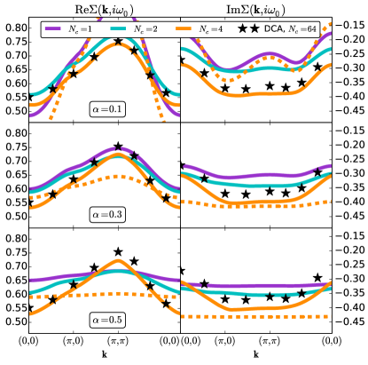
Figure S.3: Point C in the Heisenberg decoupling ($U/D=1.4$, $\delta=4\%$, $\beta D=8$). Same conventions as Fig. S.1. Stars: DCA from Ref. Wu et al., , $N_{c}=64$

In the main text, we have chosen to decouple the interaction with charge and longitudinal spin bosons (a decoupling sometimes called the “Ising” decoupling). One can alternatively use the “Heisenberg” decoupling, which consists in decomposing the interaction as follows (up to a density term):

$$Un_{i\uparrow}n_{i\downarrow}=\frac{1}{2}U^{\mathrm{ch}}n_{i}n_{i}+\frac{1}{2}U^{\mathrm{sp}}\left(s_{i}^{x}s_{i}^{x}+s_{i}^{y}s_{i}^{y}+s_{i}^{z}s_{i}^{z}\right)$$ (11)

where $s_{i}^{I}\equiv\sum_{\sigma\sigma^{\prime}}c_{i\sigma}^{\dagger}\sigma_{\sigma\sigma^{\prime}}^{I}c_{i\sigma^{\prime}}$ (with $\sigma^{I}$ the Pauli matrices). This equality holds whenever $U^{\mathrm{ch}}-3U^{\mathrm{sp}}=U$, or in other words

$$U^{\mathrm{ch}} =(3\alpha-1)U,\;\;U^{\mathrm{sp}}=(\alpha-2/3)U$$ (12)

This leads, after a Hubbard-Stratonovich transformation, to four bosonic modes, one in the charge channel and three in the spin channel (we refer the reader to Ayral and Parcollet (2016b) for more details and for the modified equations for the self-energy and impurity action).

In Figs (S.1-S.2-S.3), we show the self-energies obtained for the three characteristic points studied in the main text (A, B and C) for different values of the Fierz parameter $\alpha$ and cluster size $N_{c}$.

The observations with respect to $\alpha$ dependence are very similar to those made in the main text. This further underlines the main conclusion of the paper: even in this quite different decoupling, the results are similar to those obtained within the Ising decoupling of the main text.

Supplemental Material B Technical details of cluster TRILEX

B.1 Fourier conventions and patching details

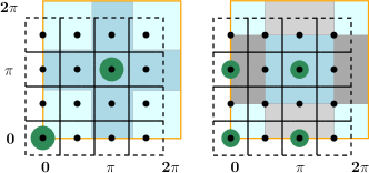
Figure S.4: Example of discretization of the Brillouin zone with $n_{\mathrm{latt}}=n_{k}\times n_{k}$ $\mathbf{k}$ points (here $n_{\mathbf{k}}=4$) for $N_{c}=2$ (left panel) and $N_{c}=4$ (right panel)

B.1.1 Spatial Fourier transforms

$\mathbf{k}$ is a Brillouin zone momentum (black dots in Fig. S.4).

Direct transforms

We define:

$$f_{\mathbf{k}} \equiv\sum_{i=1}^{n_{\mathrm{latt}}}e^{-i\mathbf{k}\cdot\mathbf{r}_{i}}f_{\mathbf{r}_{i}}$$ (13)

Reciprocal transforms

We define:

$$f_{\mathbf{r}} =\frac{1}{n_{\mathrm{latt}}}\sum_{i=1}^{n_{\mathrm{latt}}}e^{i\mathbf{k}_{i}\cdot\mathbf{r}}f_{\mathbf{k}}$$ (14)

B.1.2 Cluster Fourier transforms

$\mathbf{K}$ and $\mathbf{Q}$ are cluster momenta (green disks in Fig. S.4)

Direct transforms

We define:

$$f_{\mathbf{K}} \equiv\frac{1}{N_{c}}\sum_{ij}e^{-i\mathbf{K}\cdot(\mathbf{R}_{i}-\mathbf{R}_{j})}f_{ij}$$ (15)

$$g_{\mathbf{K},\mathbf{Q}} \equiv\frac{1}{N_{c}}\sum_{ijk}e^{-i\mathbf{K}\cdot(\mathbf{R}_{i}-\mathbf{R}_{j})-i\mathbf{Q}\cdot(\mathbf{R}_{k}-\mathbf{R}_{j})}g_{ijk}$$ (16)

with $i,j,k=1\dots N_{c}$.

Reciprocal transforms

We define:

$$f_{ij} =\sum_{\mathbf{K}}e^{i\mathbf{K}\cdot(\mathbf{R}_{i}-\mathbf{R}_{j})}f_{\mathbf{K}}$$ (17)

$$g_{ijk} =\sum_{\mathbf{K}\mathbf{Q}}e^{i\mathbf{K}(\mathbf{R}_{i}-\mathbf{R}_{j})+i\mathbf{Q}(\mathbf{R}_{k}-\mathbf{R}_{j})}g_{\mathbf{K},\mathbf{Q}}$$ (18)

where $\sum_{\mathbf{K}}f_{\mathbf{K}}$ is shorthand for $\frac{1}{N_{c}}\sum_{i=1}^{N_{c}}f_{\mathbf{K}_{i}}$.

B.1.3 Temporal Fourier transforms

$i\omega$ (resp. $i\Omega)$ denotes fermionic (resp. bosonic) Matsubara frequencies, and are shorthand for $i\omega_{n}=\frac{2n+1}{\beta}\pi$ (resp. $i\Omega_{m}=\frac{2m}{\beta}\pi$). $\beta$ is the inverse temperature.

Direct transforms

We define:

$$f_{i\omega} \equiv\int_{0}^{\beta}\mathrm{d}\tau e^{i\omega\tau}f_{\tau}$$ (19)

$$g_{i\omega,i\Omega} \equiv\iint_{0}^{\beta}\mathrm{d\tau}\mathrm{d}\tau^{\prime}e^{i\omega\tau+i\Omega\tau^{\prime}}g_{\tau,\tau^{\prime}}$$ (20)

Reciprocal transforms

We define:

$$f_{\tau} =\sum_{i\omega}e^{-i\omega\tau}f_{i\omega}$$ (21)

$$g_{\tau,\tau^{\prime}} =\sum_{i\omega}\sum_{i\Omega}e^{-i\omega\tau-i\Omega\tau^{\prime}}g_{i\omega,i\Omega}$$ (22)

Here, $\sum_{i\omega}f(i\omega)$ is shorthand for $\frac{1}{\beta}\sum_{n=-n_{\mathrm{max}}}^{n_{\mathrm{max}}-1}f(i\omega_{n})$ (and $\sum_{i\Omega}f(i\Omega)$ for $\frac{1}{\beta}\sum_{m=-m_{\mathrm{max}}}^{m_{\mathrm{max}}}f(i\Omega_{m})$).

B.1.4 Patching and discretization

In DCA, the $\mathbf{k}$ integrals can be replaced with integrals on the density of states, e.g.

$$G_{\mathbf{K}}(i\omega) =\sum_{\mathbf{k}\in\mathcal{P}_{\mathbf{K}}}\frac{1}{i\omega+\mu-\varepsilon_{\mathbf{k}}-\Sigma_{\mathrm{imp}}(\mathbf{K},i\omega)}$$

$$=\int_{-\infty}^{\infty}\mathrm{d}\varepsilon\frac{D_{\mathbf{K}}(\varepsilon)}{i\omega+\mu-\varepsilon-\Sigma_{\mathrm{imp}}(\mathbf{K},i\omega)}$$

where $D_{\mathbf{K}}(\varepsilon)\equiv\sum_{\mathbf{k}\in\mathcal{P}_{\mathbf{K}}}\delta(\varepsilon-\varepsilon_{\mathbf{k}})$ is the noninteracting density of states of patch $\mathbf{K}$. This density of states can be precomputed once and for all for a given dispersion and patches with a very large number of $\mathbf{k}$ points to obtain a very good accuracy.

By contrast, in cluster TRILEX, the self-energy is a function of $\mathbf{k}$ instead of $\mathbf{K}$, forbidding this substitution and keeping the number of $\mathbf{k}$ points finite (this number is primarily limited by memory and computation time requirements, but it can be large due to the low cost of the computation of $\Sigma(\mathbf{k},i\omega)$: we typically discretize the Brillouin zone in $n_{\mathbf{k}}\times n_{\mathbf{k}}$ points, with $n_{\mathbf{k}}=32$).

This requires extra care when defining the theta functions $\theta_{\mathbf{K}}(\mathbf{k})$ defined in a loose way in the main text. $\theta_{\mathbf{K}}(\mathbf{k})$ is precisely defined as the overlap of the area surrounding a given $\mathbf{k}$ point with the patch $\mathcal{P}_{\mathbf{K}}$, divided by the total area surrounding the $\mathbf{k}$ point. This area is illustrated in Fig. S.4 for the case $n_{\mathbf{k}}=4$. For instance, the $\mathbf{k}$ point of coordinates $(1,1)$ has $\theta_{\mathbf{K}=(0,0)}(\mathbf{k})=1/4$, while that of coordinates $(1,2)$ has $\theta_{\mathbf{K}=(0,\pi)}(\mathbf{k})=1/2$.

Correspondingly, $\sum_{\mathbf{k}\in\mathcal{P}_{\mathbf{K}}}$ is precisely defined as

$$f_{\mathbf{K}}=\sum_{\mathbf{k}\in\mathcal{P}_{\mathbf{K}}}f_{\mathbf{k}}=\frac{\sum_{i=1}^{n_{\mathbf{k}}\times n_{\mathbf{k}}}f(\mathbf{k}_{i})\theta_{\mathbf{K}}(\mathbf{k}_{i})}{\sum_{i=1}^{n_{\mathbf{k}}\times n_{\mathbf{k}}}\theta_{\mathbf{K}}(\mathbf{k}_{i})}$$ (23)

B.2 Cluster TRILEX Loop

As in Refs Ayral and Parcollet, 2015, 2016b; Vučičević et al., , we solve the cluster TRILEX equations by forward recursion, with the following steps (illustrated in Fig. S.5):

1. Start with a guess $\Sigma(\mathbf{k},i\omega)$, $P^{\eta}(\mathbf{q},i\Omega)$

2. Compute $G(\mathbf{k},i\omega)$ and $W^{\eta}(\mathbf{q},i\Omega)$ (Eqs (4)) and then $G(\mathbf{K},i\omega)$ and $W^{\eta}(\mathbf{Q},i\Omega)$ (Eqs. (10))

3. Compute $\mathcal{G}(\mathbf{K},i\omega)$ and $\mathcal{U}^{\eta}(\mathbf{Q},i\Omega)$ by substituting Eqs (9) into the impurity Dyson equations, i.e

   $$\mathcal{G}(\mathbf{K},i\omega) =\left[G_{\mathbf{K}}^{-1}(i\omega)+\Sigma_{\mathrm{imp}}(\mathbf{K},i\omega)\right]^{-1}$$ (24a)

   $$\mathcal{U}^{\eta}(\mathbf{Q},i\Omega) =\left[\left[W_{\mathbf{Q}}^{\eta}\right]^{-1}(i\Omega)+P_{\mathrm{imp}}^{\eta}(\mathbf{Q},i\Omega)\right]^{-1}$$ (24b)

4. Solve the impurity model, Eq. (6), for its exact vertex $\Lambda_{\mathrm{imp}}^{\eta}(\mathbf{K},\mathbf{Q};i\omega,i\Omega)$ (see Section B.3 for more details).

5. Compute $\Sigma(\mathbf{k},i\omega)$ and $P^{\eta}(\mathbf{q},i\Omega)$ (Eqs (5))

6. Go back to step 2 until convergence of $\Sigma$ and $P^{\eta}$.

As in Refs Ayral and Parcollet, 2015; Vučičević et al., , and as justified in Ref. Ayral and Parcollet, 2016b for the single-site impurity case, in the equations presented in the main text and in the loop presented above, we have implicitly approximated the impurity’s electron-boson vertex with the bare electron-boson vertex or, in other words, we have assumed the $\zeta$ function, introduced in Ref. Ayral and Parcollet, 2016b, to be negligible.

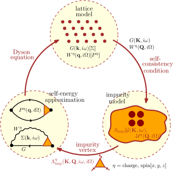
Figure S.5: The cluster TRILEX loop

B.3 Solution of the Impurity Model

B.3.1 Impurity solver

The impurity model, defined by Eq. (6), is solved using a continuous-time quantum Monte-Carlo algorithmRubtsov et al. (2005). For $N_{c}=1$, we refer the reader to Ref. Ayral and Parcollet, 2016b for details. For $N_{c}>1$, contrary to the single-site case, the densities $n_{i}^{I}$ are no longer good quantum numbers due to the intra-cluster hopping terms. This precludes the use of the hybridization expansion algorithms, which can be used with retarded interactions only if the operators involved in the retarded interactions are good quantum numbers, and in which only correlators between operators which are good quantum numbers can be easily measured. We therefore use an interaction-expansion (CT-INT) algorithm, described e.g. in Ref. Gull et al., 2011. Here, for the measurement of the three-point function $\tilde{\chi}_{\mathrm{imp}}^{3,\sigma\sigma^{\prime}}(i,j,k;\tau,\tau^{\prime})$ (defined in Eq. (30) below), we use a straightforward operator-insertion method.

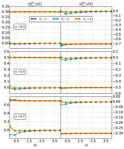
Figure S.6: Retarded interaction $\mathcal{U}_{ij}^{\eta}(i\Omega)$ in the charge (left column) and spin (right column) channels, for $\alpha=0.3$ (top row), $0.5$ (middle row), $0.7$ (bottom row), at point B ($U/D=1$, $\delta=20\%$, $\beta D=16$, $t^{\prime}=0$, Ising decoupling). Dots: local component ($i,j=0,0$). Triangles: nearest-neighbor component ($i,j=0,1$, for $N_{c}=2$ and $N_{c}=4$ only). Squares: next-nearest-neighbor component ($i,j=0,3$, for $N_{c}=4$ only).

We observe that in all the parameter regimes studied in the main text (points A, B and C), the interactions $\mathcal{U}_{ij}^{I}(\tau)$ are static and local to a very good approximation:

$$\mathcal{U}_{ij}^{I}(\tau)\approx U^{I}\delta_{ij}\delta_{\tau}$$ (25)

This is illustrated in Fig. S.6 for point B. Thus, in practice, we do not have to use the retarded interactions. This simplifies the numerical computation since the dependence of the Monte-Carlo sign problem on CT-INT’s density-shifting parameter $\alpha_{\sigma}(s)$ (see e.g. Eq. (145) of Ref. Gull et al., 2011) is less simple than in the case of static interactions.

B.3.2 Computation of $G_{\mathrm{imp}}(\mathbf{K},i\omega)$ and $W_{\mathrm{imp}}(\mathbf{Q},i\Omega)$

$G_{\mathrm{imp}}(\mathbf{K},i\omega)$ and $W_{\mathrm{imp}}(\mathbf{Q},i\Omega)$ are obtained by computing the spatial and temporal Fourier transforms (defined in Section B.1) $G_{\mathrm{imp}}(\mathbf{K},i\omega)$ and $\chi_{\mathrm{imp}}^{\sigma\sigma^{\prime}}(\mathbf{Q},i\Omega)$ of the impurity’s Green’s function and density-density response functions:

$$G_{\mathrm{imp}}(i,j;\tau) \equiv-\langle Tc_{i}(\tau)c_{j}^{\dagger}(0)\rangle_{\mathrm{imp}}$$ (26a)

$$\chi_{\mathrm{imp}}^{\sigma\sigma^{\prime}}(i,j;\tau) \equiv\langle Tn_{i\sigma}(\tau)n_{j\sigma^{\prime}}(0)\rangle_{\mathrm{imp}}$$ (26b)

and by using the identity

$$W_{\mathrm{imp}}^{\eta}(\mathbf{Q},i\Omega)=$$ (27)

$$\mathcal{U}^{\eta}(\mathbf{Q},i\Omega)-\mathcal{U}^{\eta}(\mathbf{Q},i\Omega)\chi_{\mathrm{imp}}^{\eta,\mathrm{conn}}(\mathbf{Q},i\Omega)\mathcal{U}^{\eta}(\mathbf{Q},i\Omega)$$

where the passage from spin ($\sigma,\sigma^{\prime}$) to channel ($\eta$) indices is done using the expressions:

$$\chi_{\mathrm{imp}}^{\eta=\mathrm{ch}} \equiv 2(\chi_{\mathrm{imp}}^{\uparrow\uparrow}+\chi_{\mathrm{imp}}^{\uparrow\downarrow})$$ (28a)

$$\chi_{\mathrm{imp}}^{\eta=\mathrm{sp}} \equiv 2(\chi_{\mathrm{imp}}^{\uparrow\uparrow}-\chi_{\mathrm{imp}}^{\uparrow\downarrow})$$ (28b)

and the connected component is:

$$\chi_{\mathrm{imp}}^{\eta,\mathrm{conn}}(i,j;i\Omega)\equiv\chi_{\mathrm{imp}}^{\eta,\mathrm{conn}}(i,j;i\Omega)-\langle n_{i}^{\eta}\rangle\langle n_{j}^{\eta}\rangle\beta\delta_{i\Omega}$$ (29)

B.3.3 Computation of the cluster vertex $\Lambda_{\mathrm{imp}}^{\eta}(\mathbf{K},\mathbf{Q};i\omega,i\Omega)$

The computation of $\Lambda_{\mathrm{imp}}^{\eta}(\mathbf{K},\mathbf{Q};i\omega,i\Omega)$ is done by measuring the three-point function

$$\tilde{\chi}_{\mathrm{imp}}^{3,\sigma,\sigma^{\prime}}(i,j,k;\tau,\tau^{\prime})\equiv\langle Tc_{i\sigma}(\tau)c_{j\sigma}^{\dagger}(0)n_{k\sigma^{\prime}}(\tau^{\prime})\rangle_{\mathrm{imp}}$$ (30)

The vertex, written in cluster coordinates $\mathbf{R}_{i},\mathbf{R}_{j},\mathbf{R}_{k}$, is then computed as:

$$\Lambda^{\eta}(i,j,k;i\omega,i\Omega)\equiv\sum_{pqr}G_{\mathrm{imp}}^{-1}(p,j;i\omega+i\Omega)G_{\mathrm{imp}}^{-1}(i,q;i\omega)$$

$$\;\;\times\left[1-\mathcal{U}^{\eta}\chi_{\mathrm{imp}}^{\eta}\right]^{-1}(k,r;i\Omega)\tilde{\chi}_{\mathrm{imp}}^{3,\eta,\mathrm{conn}}(q,p,r;i\omega,i\Omega)$$ (31)

with the expression in the charge and spin channel:

$$\tilde{\chi}_{\mathrm{imp}}^{3,\eta=\mathrm{ch}}\equiv\tilde{\chi}_{\mathrm{imp}}^{3,\uparrow\uparrow}+\tilde{\chi}_{\mathrm{imp}}^{3,\uparrow\downarrow}$$ (32a)

$$\tilde{\chi}_{\mathrm{imp}}^{3,\eta=\mathrm{sp}}\equiv\tilde{\chi}_{\mathrm{imp}}^{3,\uparrow\uparrow}-\tilde{\chi}_{\mathrm{imp}}^{3,\uparrow\downarrow}$$ (32b)

and the connected component defined as:

$$\tilde{\chi}_{\mathrm{imp}}^{3,\eta,\mathrm{conn}}(i,j,k;i\omega,i\Omega)\equiv$$ (33)

$$\;\;\tilde{\chi}_{\mathrm{imp}}^{3,\eta}(i,j,k;i\omega,i\Omega)+G_{\mathrm{imp}}(i,j;i\omega)n_{k}^{\eta}\beta\delta_{i\Omega}$$

$\Lambda^{\eta}(i,j,k;i\omega,i\Omega)$ is then Fourier-transformed to $\Lambda_{\mathrm{imp}}^{\eta}(\mathbf{K},\mathbf{Q};i\omega,i\Omega)$ (see Section B.1, Eq. (16)).

In practice, instead of directly performing a temporal Fourier transform to compute $\tilde{\chi}_{\mathrm{imp}}^{3,\sigma\sigma^{\prime}}(i,j,k;i\omega,i\Omega)$ from $\tilde{\chi}_{\mathrm{imp}}^{3,\sigma\sigma^{\prime}}(i,j,k;\tau,\tau^{\prime})$, we first compute the connected component $\tilde{\chi}_{\mathrm{imp}}^{3,\eta,\mathrm{conn}}(i,j,k;\tau,\tau^{\prime})$ [defined in Eq. (33)], which is smooth and without discontinuities, perform a cubic spline interpolation of it, and then Fourier transform it to Matsubara frequencies. This allows us to use a small number (typically $n_{\tau}=n_{\tau^{\prime}}=100$) of $\tau,\tau^{\prime}$ points in the measurement.

B.4 Self-energy decomposition

In this section, we show that the coarse-grainings introduced for the vertex allow for a numerically convenient decomposition of $\Sigma$ and $P$.

Following a procedure very similar to that described in section II.D.3 of Ref. Ayral and Parcollet, 2016b, we decompose Eqs (5) as follows:

$$\Sigma(\mathbf{k},i\omega)=\Sigma_{\mathrm{imp}}(i,j=0,0;i\omega)$$ (34a)

$$\;\;\;-\sum_{\eta}m_{\eta}\sum_{\mathbf{K},\mathbf{Q}}\sum_{\mathbf{q},i\Omega}\tilde{G}_{\mathbf{k}+\mathbf{q},i\omega+i\Omega}^{\mathbf{K}+\mathbf{Q}}\tilde{W}_{\mathbf{q},i\Omega}^{\eta,\mathbf{Q}}\Lambda_{\mathrm{imp}}^{\eta}(\mathbf{K},\mathbf{Q};i\omega,i\Omega)$$

$$P^{\eta}(\mathbf{q},i\Omega)=P_{\mathrm{imp}}^{\eta}(i,j=0,0;i\Omega)$$ (34b)

$$\;\;\;+2\sum_{\mathbf{K},\mathbf{Q}}\sum_{\mathbf{k},i\omega}\tilde{G}_{\mathbf{k}+\mathbf{q},i\omega+i\Omega}^{\mathbf{K}+\mathbf{Q}}\tilde{G}_{\mathbf{k},i\omega}^{\mathbf{K}}\Lambda_{\mathrm{imp}}^{\eta}(\mathbf{K},\mathbf{Q};i\omega,i\Omega)$$

where we have defined the nonlocal components:

$$\tilde{X}(\mathbf{k},i\omega)\equiv X(\mathbf{k},i\omega)-\sum_{\mathbf{k}}X(\mathbf{k},i\omega)$$ (35)

with $X=G$ or $W$.

Indeed, decomposing Eq. (5a) using Eq. (35), and expanding, one obtains four terms, two of which vanish. The two remaining terms are given in Eq. (34a). The first term is given by $\Sigma_{\mathrm{imp}}(00,i\omega)$:

$$-\sum_{\eta}m_{\eta}\sum_{\mathbf{K},\mathbf{Q}}\sum_{i\Omega}\left\{\sum_{\mathbf{k}^{\prime}}G_{i\omega+i\Omega}(\mathbf{k}^{\prime})\theta_{\mathbf{K}+\mathbf{Q}}(\mathbf{k}^{\prime})\right\}$$

$$\;\;\times\left\{\sum_{\mathbf{q}^{\prime}}W_{i\Omega}(\mathbf{q}^{\prime})\theta_{\mathbf{Q}}(\mathbf{q}^{\prime})\right\}\Lambda_{\mathrm{imp}}^{\eta}(\mathbf{K},\mathbf{Q};i\omega,i\Omega)$$ (36)

$$=-\sum_{\eta}m_{\eta}\sum_{i\Omega}\sum_{\mathbf{q}^{\prime}}\sum_{\mathbf{k}^{\prime}}\left\{G_{i\omega+i\Omega}(\mathbf{k}^{\prime}+\mathbf{q}^{\prime})\right\}\left\{W_{i\Omega}(\mathbf{q}^{\prime})\right\}$$

$$\;\;\times\sum_{\mathbf{K}\mathbf{Q}}\theta_{\mathbf{K}+\mathbf{Q}}(\mathbf{k}^{\prime}+\mathbf{q}^{\prime})\theta_{\mathbf{Q}}(\mathbf{q}^{\prime})\Lambda_{\mathrm{imp}}^{\eta}(\mathbf{K},\mathbf{Q};i\omega,i\Omega)$$ (37)

$$=-\sum_{\mathbf{k}^{\prime}}\sum_{\eta}m_{\eta}\sum_{\mathbf{q}^{\prime}}\sum_{i\Omega}G_{i\omega+i\Omega}(\mathbf{k}^{\prime}+\mathbf{q}^{\prime})W_{i\Omega}(\mathbf{q}^{\prime})\Lambda_{\mathbf{k}^{\prime},\mathbf{q}^{\prime}}^{\eta}(i\omega,i\Omega)$$

$$=\sum_{\mathbf{k}^{\prime}}\Sigma(\mathbf{k}^{\prime},i\omega)$$

$$=\Sigma(\mathbf{R}=0,i\omega)$$

$$=\Sigma_{\mathrm{imp}}(0,0;i\omega)$$ (38)

A similar result holds for $P$.

In the second terms of Eqs (34a-34b), the summands decay fast for large Matsubara frequencies thanks to the fast decay of the nonlocal component $\tilde{G}(\mathbf{k},i\omega)$ and $\tilde{W}(\mathbf{q},i\Omega)$.

As in Ref. Ayral and Parcollet, 2016b, we furthermore split $\Lambda$ into a “regular part” $\Lambda^{\eta,\mathrm{reg}}$ which vanishes at large frequencies

$$\Lambda^{\eta,\mathrm{reg}}(i,j,k;i\omega,i\Omega)=\Lambda^{\eta}(i,j,k;i\omega,i\Omega)-l^{\eta}(i,j,k;i\Omega)$$ (39)

and a remainder $l^{\eta}(i\Omega)$ corresponding to the high-frequency asymptotics of the three-point function:

$$l^{\eta}(i,j,k;i\Omega)\equiv\sum_{p}\left[1-\mathcal{U}^{\eta}\chi^{\eta}\right]^{-1}(k,p;i\Omega)\delta_{ij}$$ (40)

The term containing $\Lambda^{\eta,\mathrm{reg}}(i,j,k;i\omega,i\Omega)$ has a quickly decaying summand thanks to $\tilde{G}$, $\tilde{W}$ and $\Lambda^{\mathrm{reg}}$. We compute it in Matsubara frequencies and real space after a fast Fourier transform of $\tilde{G}$ and $\tilde{W}$ (see Eq (14)). This is the bottleneck of the computation of the self-energy as it scales as $O(N_{\omega}^{2}N_{k}\log N_{k}N_{c}^{2})$ (where $N_{\omega}$ is the number of Matsubara frequencies used and $N_{k}$ the number of $\mathbf{k}$ points in the disctretized first Brillouin zone). The term containing $l^{\eta}(i,j,k;i\Omega)$ can be computed entirely in imaginary time and real space, with a computational complexity of $O(N_{\omega}\log N_{\omega}N_{k}\log N_{k}N_{c}^{2})$.

Supplemental Material C Supplementary data

C.1 Additional data for the Fierz criterion: $\alpha$-dependence of $\mathrm{Im}\Sigma$

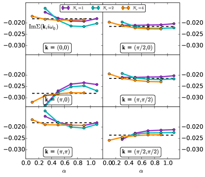
Figure S.7: Dependence of $\mathrm{Im}\Sigma(\mathbf{k},i\omega_{0})$ on the Fierz parameter $\alpha$ for different $\mathbf{k}$ points at point A ($U/D=0.5$, $\delta=0\%$, $\beta D=16$, $t^{\prime}=0$, Ising decoupling).

In Figure S.7, we complement the data of Fig. 3 of the main text by giving the data for the imaginary part. Similarly to the real part, the imaginary part shows plateaus for given ranges of $\alpha$ which are more pronounced for $N_{c}=4$, which is the cluster size for which the self-energy is the closest to the exact benchmark result.

C.2 Continuity of the self-energy

In Fig. S.8, we show the lowest Matsubara component of the self-energy obtained in the dynamical cluster approximation (DCA) and the one obtained within cluster TRILEX, using Eq. (34a). While the DCA self-energy is piecewise constant in the Brillouin zone (with discontinuities at the patch edges), the cluster TRILEX self-energy is continuous by construction, similarly to what is achieved by the DCA⁺ methodStaar et al. (2013, 2014), but without arbitrary interpolation schemes.

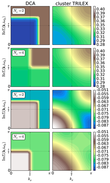
Figure S.8: $\Sigma(\mathbf{k},i\omega_{0})$ in the upper quadrant of the first Brillouin zone, at point B ($U/D=1$, $\delta=20\%$, $\beta D=16$, $t^{\prime}=0$, $\alpha=0.5$, Ising decoupling). Left column: DCA, right column: cluster TRILEX. First two rows: real part, last two rows: imaginary part. Odd rows: $N_{c}=2$, even rows: $N_{c}=4$.

C.3 Local components of $\mathrm{Im}G$ and $\mathrm{Im}\Sigma$

In Fig. S.9, we display the local components $G_{\mathrm{loc}}$ and $\Sigma_{\mathrm{imp}}$ and compare them to benchmark results obtained with DCA ($N_{c}=50$, Ref. LeBlanc et al., 2015). The $N_{c}=4$ cluster TRILEX data is the closest to the benchmark data, irrespective of the value of $\alpha$.

Figure S.9: (Point B: $U/D=1$, $\delta=20\%$, $\beta D=16$, $t^{\prime}=0$, Ising decoupling). Imaginary part of the local components of $G_{\mathrm{loc}}$ (left column) and $\Sigma_{\mathrm{imp}}$ (right column) for for $\alpha=0.3$ (top row), $0.5$ (middle row), $0.7$ (bottom row) and different $N_{c}$. Solid lines: TRILEX. Dashed lines: $GW$+EDMFT ($N_{c}=4$). Black stars: DCA result from Ref. LeBlanc et al., 2015, $N_{c}=50$.

C.4 Vertex

C.4.1 Momentum dependence of the vertex

In Figures S.10 and S.11, we show the dependence of the vertex on the cluster momenta $\mathbf{K}$ and $\mathbf{Q}$ for points A and C (point B is shown in the main text).

C.4.2 Cluster-site dependence of the vertex

In Figures S.12, S.13 and S.14, we show all the inequivalent vertex components $\Lambda_{\mathrm{imp}}(i,j,k;i\omega,i\Omega)$ for the three regimes of parameters (respectively point A, B and C) studied in the main text. While the largest component is the local component ($i,j,k=0,0,0$), some nonlocal components are non-negligible.

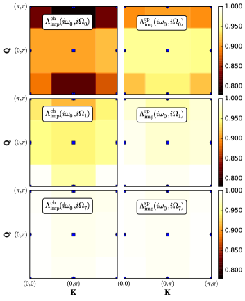
Figure S.10: Weak-coupling parameters (Point A, $U/D=0.5$, $\delta=0\%$, $\beta D=16$, $t^{\prime}=0$, $\alpha=0.5$, Ising decoupling). Same conventions as Fig. 6 of the main text.

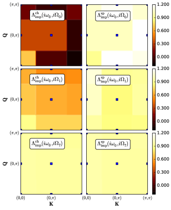
Figure S.11: Strong-coupling parameters (Point C, $U/D=1.4$, $\delta=4\%$, $\beta D=8$, $t^{\prime}/t=-0.3$, $\alpha=0.5$, Ising decoupling). Same conventions as Fig. 6 of the main text.

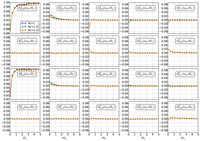
Figure S.12: Weak-coupling parameters (Point A, $U/D=0.5$, $\delta=0\%$, $\beta D=16$, $t^{\prime}=0$), $\alpha=0.5$, Ising decoupling. Impurity cluster vertex $\Lambda_{\mathrm{imp}}^{\eta}(i,j,k;i\omega,i\Omega)$ in the charge (first two rows) and spin (last two rows) channels, at fixed fermionic Matsubara frequency $\omega_{0}$. See Fig 1 for a definition of the cluster coordinates $\mathbf{R}_{i},\mathbf{R}_{j}$ and $\mathbf{R}_{k}$ denoted by the indices $i,j,k$.

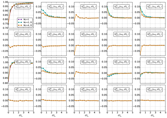
Figure S.13: Intermediate-coupling parameters (point B, $U/D=1$, $\delta=20\%$, $\beta D=16$, $t^{\prime}=0$), $\alpha=0.5$, Ising decoupling. Impurity cluster vertex $\Lambda_{\mathrm{imp}}^{\eta}(i,j,k;i\omega,i\Omega)$ in the charge and spin channels, at fixed fermionic Matsubara frequency $\omega_{0}$.

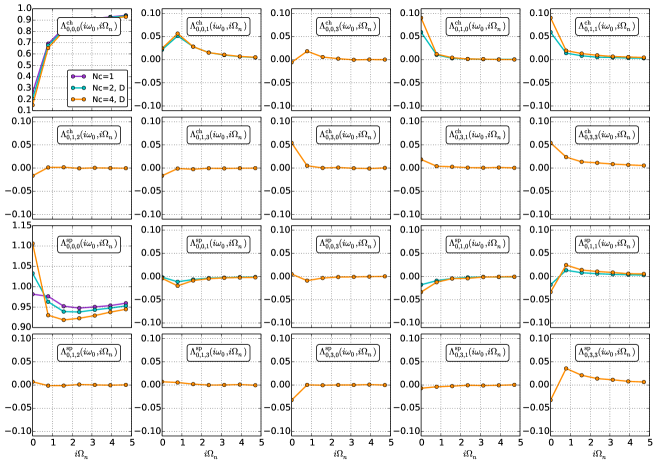
Figure S.14: Strong-coupling parameters (Point C, $U/D=1.4$, $\delta=4\%$, $\beta D=8$, $t^{\prime}/t=-0.3$), $\alpha=0.5$, Ising decoupling. Impurity cluster vertex $\Lambda_{\mathrm{imp}}^{\eta}(i,j,k;i\omega,i\Omega)$ in the charge and spin channels, at fixed fermionic Matsubara frequency $\omega_{0}$.

References

- Chubukov et al. (2002) A. V. Chubukov, D. Pines, and J. Schmalian, in Superconductivity (Springer Berlin Heidelberg, Berlin, Heidelberg, 2002) Chap. 22, pp. 1349–1413.
- Onufrieva and Pfeuty (2009) F. Onufrieva and P. Pfeuty, Physical Review Letters 102, 207003 (2009).
- Metlitski and Sachdev (2010) M. A. Metlitski and S. Sachdev, Physical Review B 82, 075128 (2010).
- Efetov et al. (2013) K. B. Efetov, H. Meier, and C. Pépin, Nature Physics 9, 442 (2013).
- Onufrieva and Pfeuty (2012) F. Onufrieva and P. Pfeuty, Physical Review Letters 109, 257001 (2012).
- Scalapino (2012) D. J. Scalapino, Reviews of Modern Physics 84, 1383 (2012).
- Wang and Chubukov (2014) Y. Wang and A. Chubukov, Physical Review B 90, 035149 (2014).
- Wang et al. (2016) Y. Wang, A. Abanov, B. L. Altshuler, E. A. Yuzbashyan, and A. V. Chubukov, Physical Review Letters 117, 157001 (2016).
- Bickers and Scalapino (1989) N. Bickers and D. Scalapino, Annals of Physics 206251, 206 (1989).
- Hedin (1965) L. Hedin, Physical Review 139, 796 (1965).
- Hedin (1999) L. Hedin, Journal of Physics: Condensed Matter 489 (1999).
- Eliashberg (1960) G. M. Eliashberg, Sov. Phys. JETP 11, 696 (1960).
- Jaeckel and Wetterich (2003) J. Jaeckel and C. Wetterich, Physical Review D 68, 025020 (2003).
- Baier et al. (2004) T. Baier, E. Bick, and C. Wetterich, Physical Review B 70, 125111 (2004).
- Bartosch et al. (2009) L. Bartosch, H. Freire, J. J. R. Cardenas, and P. Kopietz, Journal of Physics: Condensed Matter 21, 305602 (2009).
- Borejsza and Dupuis (2003) K. Borejsza and N. Dupuis, Europhysics Letters (EPL) 63, 722 (2003).
- Borejsza and Dupuis (2004) K. Borejsza and N. Dupuis, Physical Review B 69, 085119 (2004).
- Dupuis (2002) N. Dupuis, Physical Review B 65, 245118 (2002).
- Anderson (1987) P. W. Anderson, Science 235, 1196 (1987).
- Georges et al. (1996) A. Georges, G. Kotliar, W. Krauth, and M. J. Rozenberg, Reviews of Modern Physics 68, 13 (1996).
- Hettler et al. (1998) M. H. Hettler, A. N. Tahvildar-Zadeh, M. Jarrell, T. Pruschke, and H. R. Krishnamurthy, Physical Review B 58, R7475 (1998).
- Hettler et al. (1999) M. H. Hettler, M. Mukherjee, M. Jarrell, and H. R. Krishnamurthy, Physical Review B 61, 12739 (1999).
- Lichtenstein and Katsnelson (2000) A. I. Lichtenstein and M. I. Katsnelson, Physical Review B 62, R9283 (2000).
- Kotliar et al. (2001) G. Kotliar, S. Savrasov, G. Pálsson, and G. Biroli, Physical Review Letters 87, 186401 (2001).
- Maier et al. (2005a) T. A. Maier, M. Jarrell, T. Pruschke, and M. H. Hettler, Reviews of Modern Physics 77, 1027 (2005a).
- Kyung et al. (2009) B. Kyung, D. Sénéchal, and A.-M. S. Tremblay, Physical Review B 80, 205109 (2009).
- Sordi et al. (2012a) G. Sordi, P. Sémon, K. Haule, and A.-M. S. Tremblay, Physical Review Letters 108, 216401 (2012a).
- Civelli et al. (2008) M. Civelli, M. Capone, A. Georges, K. Haule, O. Parcollet, T. D. Stanescu, and G. Kotliar, Physical Review Letters 100, 046402 (2008).
- Ferrero et al. (2010) M. Ferrero, O. Parcollet, a. Georges, G. Kotliar, and D. N. Basov, Physical Review B 82, 054502 (2010).
- Gull et al. (2013) E. Gull, O. Parcollet, and A. J. Millis, Physical Review Letters 110, 216405 (2013).
- Macridin et al. (2004) A. Macridin, M. Jarrell, and T. A. Maier, Physical Review B 70, 113105 (2004).
- Maier et al. (2004) T. A. Maier, M. Jarrell, A. Macridin, and C. Slezak, Physical Review Letters 92, 027005 (2004).
- Maier et al. (2005b) T. A. Maier, M. Jarrell, T. C. Schulthess, P. R. C. Kent, and J. B. White, Physical Review Letters 95, 237001 (2005b).
- Maier et al. (2006) T. Maier, M. Jarrell, and D. Scalapino, Physical Review Letters 96, 047005 (2006).
- Gull et al. (2010) E. Gull, M. Ferrero, O. Parcollet, A. Georges, and A. J. Millis, Physical Review B 82, 155101 (2010).
- Yang et al. (2011a) S. X. Yang, H. Fotso, S. Q. Su, D. Galanakis, E. Khatami, J. H. She, J. Moreno, J. Zaanen, and M. Jarrell, Physical Review Letters 106, 047004 (2011a).
- Macridin and Jarrell (2008) A. Macridin and M. Jarrell, Physical Review B 78, 241101(R) (2008).
- Macridin et al. (2006) A. Macridin, M. Jarrell, T. Maier, P. R. C. Kent, and E. D’Azevedo, Physical Review Letters 97, 036401 (2006).
- Jarrell et al. (2001) M. Jarrell, T. A. Maier, C. Huscroft, and S. Moukouri, Physical Review B 64, 195130 (2001).
- Parcollet et al. (2004) O. Parcollet, G. Biroli, and G. Kotliar, Physical Review Letters 92, 226402 (2004).
- Werner et al. (2009) P. Werner, E. Gull, O. Parcollet, and A. J. Millis, Physical Review B 80, 045120 (2009).
- Biroli et al. (2004) G. Biroli, O. Parcollet, and G. Kotliar, Physical Review B 69, 205108 (2004).
- Bergeron et al. (2011) D. Bergeron, V. Hankevych, B. Kyung, and A.-M. S. Tremblay, Physical Review B 84, 085128 (2011).
- Kyung et al. (2004) B. Kyung, V. Hankevych, A.-M. Daré, and A.-M. Tremblay, Physical Review Letters 93, 147004 (2004).
- Kyung et al. (2006) B. Kyung, S. S. Kancharla, D. Sénéchal, A.-M. S. Tremblay, M. Civelli, and G. Kotliar, Physical Review B 73, 165114 (2006).
- Okamoto et al. (2010) S. Okamoto, D. Sénéchal, M. Civelli, and A.-M. S. Tremblay, Physical Review B 82, 180511 (2010).
- Sordi et al. (2010) G. Sordi, K. Haule, and A.-M. S. Tremblay, Physical Review Letters 104, 226402 (2010).
- Sordi et al. (2012b) G. Sordi, P. Sémon, K. Haule, and A.-M. S. Tremblay, Scientific Reports 2, 547 (2012b).
- Civelli et al. (2005) M. Civelli, M. Capone, S. S. Kancharla, O. Parcollet, and G. Kotliar, Physical Review Letters 95, 106402 (2005).
- Ferrero et al. (2008) M. Ferrero, P. S. Cornaglia, L. De Leo, O. Parcollet, G. Kotliar, and A. Georges, Europhysics Letters 85, 57009 (2008).
- Ferrero et al. (2009) M. Ferrero, P. Cornaglia, L. De Leo, O. Parcollet, G. Kotliar, and A. Georges, Physical Review B 80, 064501 (2009).
- Gull et al. (2009) E. Gull, O. Parcollet, P. Werner, and A. J. Millis, Physical Review B 80, 245102 (2009).
- Chen et al. (2015) X. Chen, J. P. F. LeBlanc, and E. Gull, Physical Review Letters 115, 116402 (2015).
- Chen et al. (2017) X. Chen, J. P. F. LeBlanc, and E. Gull, Nature Communications 8, 14986 (2017).
- LeBlanc et al. (2015) J. P. F. LeBlanc, A. E. Antipov, F. Becca, I. W. Bulik, G. K.-L. Chan, C.-M. Chung, Y. Deng, M. Ferrero, T. M. Henderson, C. A. Jiménez-Hoyos, E. Kozik, X.-W. Liu, A. J. Millis, N. V. Prokof’ev, M. Qin, G. E. Scuseria, H. Shi, B. V. Svistunov, L. F. Tocchio, I. S. Tupitsyn, S. R. White, S. Zhang, B.-X. Zheng, Z. Zhu, and E. Gull, Physical Review X 5, 041041 (2015).
- Gunnarsson et al. (2015) O. Gunnarsson, T. Schäfer, J. P. F. LeBlanc, E. Gull, J. Merino, G. Sangiovanni, G. Rohringer, and A. Toschi, Physical Review Letters 114, 236402 (2015).
- (57) O. Gunnarsson, T. Schäfer, J. P. F. LeBlanc, J. Merino, G. Sangiovanni, G. Rohringer, and A. Toschi, arXiv:1604.01614 .
- (58) W. Wu, M. Ferrero, A. Georges, and E. Kozik, arXiv:1608.08402 .
- (59) G. Rohringer, H. Hafermann, A. Toschi, A. A. Katanin, A. E. Antipov, M. I. Katsnelson, A. I. Lichtenstein, A. N. Rubtsov, and K. Held, arXiv:1705.00024 .
- Biermann et al. (2003) S. Biermann, F. Aryasetiawan, and A. Georges, Physical Review Letters 90, 086402 (2003).
- Sun and Kotliar (2002) P. Sun and G. Kotliar, Physical Review B 66, 085120 (2002).
- Sun and Kotliar (2004) P. Sun and G. Kotliar, Physical Review Letters 92, 196402 (2004).
- Ayral et al. (2012) T. Ayral, P. Werner, and S. Biermann, Physical Review Letters 109, 226401 (2012).
- Ayral et al. (2013) T. Ayral, S. Biermann, and P. Werner, Physical Review B 87, 125149 (2013).
- Biermann (2014) S. Biermann, Journal of physics. Condensed matter : an Institute of Physics journal 26, 173202 (2014).
- (66) T. Ayral, S. Biermann, P. Werner, and L. V. Boehnke, arXiv:1701.07718 .
- Rubtsov et al. (2008) A. N. Rubtsov, M. I. Katsnelson, and A. I. Lichtenstein, Physical Review B 77, 033101 (2008).
- Rubtsov et al. (2012) A. N. Rubtsov, M. I. Katsnelson, and A. I. Lichtenstein, Annals of Physics 327, 1320 (2012).
- van Loon et al. (2014) E. G. C. P. van Loon, A. I. Lichtenstein, M. I. Katsnelson, O. Parcollet, and H. Hafermann, Physical Review B 90, 235135 (2014).
- Stepanov et al. (2016) E. A. Stepanov, E. G. C. P. van Loon, A. A. Katanin, A. I. Lichtenstein, M. I. Katsnelson, and A. N. Rubtsov, Physical Review B 93, 045107 (2016).
- Toschi et al. (2007) A. Toschi, A. Katanin, and K. Held, Physical Review B 75, 045118 (2007).
- Katanin et al. (2009) A. Katanin, A. Toschi, and K. Held, Physical Review B 80, 075104 (2009).
- Schäfer et al. (2015) T. Schäfer, F. Geles, D. Rost, G. Rohringer, E. Arrigoni, K. Held, N. Blümer, M. Aichhorn, and A. Toschi, Physical Review B 91, 125109 (2015).
- Valli et al. (2015) A. Valli, T. Schäfer, P. Thunström, G. Rohringer, S. Andergassen, G. Sangiovanni, K. Held, and A. Toschi, Physical Review B 91, 115115 (2015).
- Li et al. (2016) G. Li, N. Wentzell, P. Pudleiner, P. Thunström, and K. Held, Physical Review B 93, 165103 (2016).
- Rohringer and Toschi (2016) G. Rohringer and A. Toschi, Physical Review B 94, 125144 (2016).
- Ayral and Parcollet (2016a) T. Ayral and O. Parcollet, Physical Review B 94, 075159 (2016a).
- Hafermann et al. (2008) H. Hafermann, S. Brener, A. N. Rubtsov, M. I. Katsnelson, and A. I. Lichtenstein, JETP Letters 86, 677 (2008).
- Slezak et al. (2009) C. Slezak, M. Jarrell, T. Maier, and J. Deisz, Journal of Physics: Condensed Matter 21, 435604 (2009).
- Yang et al. (2011b) S. X. Yang, H. Fotso, H. Hafermann, K. M. Tam, J. Moreno, T. Pruschke, and M. Jarrell, Physical Review B 84, 155106 (2011b).
- Ayral and Parcollet (2015) T. Ayral and O. Parcollet, Physical Review B 92, 115109 (2015).
- Ayral and Parcollet (2016b) T. Ayral and O. Parcollet, Physical Review B 93, 235124 (2016b).
- (83) J. Vučičević, T. Ayral, and O. Parcollet, arXiv:1705.08332 .
- Note (1) See Suppl. Mat. I for another choice.
- Park et al. (2008) H. Park, K. Haule, and G. Kotliar, Physical Review Letters 101, 186403 (2008).
- Blankenbecler et al. (1981) R. Blankenbecler, D. J. Scalapino, and R. L. Sugar, Physical Review D 24, 2278 (1981).
- Note (2) This also holds for other HS decouplings, Suppl. Mat. I.
- Parcollet et al. (2015) O. Parcollet, M. Ferrero, T. Ayral, H. Hafermann, P. Seth, and I. S. Krivenko, Computer Physics Communications 196, 398 (2015).
- Rubtsov et al. (2005) A. N. Rubtsov, V. V. Savkin, and A. I. Lichtenstein, Physical Review B 72, 035122 (2005).
- Gull et al. (2011) E. Gull, A. J. Millis, A. I. Lichtenstein, A. N. Rubtsov, M. Troyer, and P. Werner, Reviews of Modern Physics 83, 349 (2011).
- Staar et al. (2013) P. Staar, T. Maier, and T. C. Schulthess, Physical Review B 88, 115101 (2013).
- Staar et al. (2014) P. Staar, T. Maier, and T. C. Schulthess, Physical Review B 89, 195133 (2014).