Sparse Stochastic Bandits

Abstract

In the classical multi-armed bandit problem, $d$ arms are available to the decision maker who pulls them sequentially in order to maximize his cumulative reward. Guarantees can be obtained on a relative quantity called regret, which scales linearly with $d$ (or with $\sqrt{d}$ in the minimax sense). We here consider the sparse case of this classical problem in the sense that only a small number of arms, namely $s<d$, have a positive expected reward. We are able to leverage this additional assumption to provide an algorithm whose regret scales with $s$ instead of $d$. Moreover, we prove that this algorithm is optimal by providing a matching lower bound – at least for a wide and pertinent range of parameters that we determine – and by evaluating its performance on simulated data.

1 Introduction

We consider the celebrated stochastic multi-armed bandit problem Robbins (1985), where a decision maker sequentially samples from $d\geqslant 1$ processes, also called arms, aiming at maximizing its cumulative reward. Specifically, those arms are characterized by their distributions $\nu_{1},\dots,\nu_{d}$ and pulling arm $i\in[d]:=\{1,...,d\}$ at time $t$ yields a reward $X_{i}(t)\sim\nu_{i}$, the sequence $(X_{i}(t))_{t\geqslant 1}$ being assumed to be i.i.d. There are many motivations behind the study of those models, ranging from random clinical trials, to maximization of the click through rate, portfolio optimization, etc.

An algorithm (or policy) maps anterior observations to the next arm $I(t)\in[d]$ to be pulled. The performance of a given algorithm is evaluated by its cumulative regret $\operatorname{Reg}(T)$ defined as the difference between the rewards gathered by the sequence $(I(t))_{1\leqslant t\leqslant T}$ and those that might have been obtained in expectation by always behaving optimally, that is, by pulling the arm with maximal mean $\mu_{i}:=\mathbb{E}_{\nu_{i}}[X]$ at each round:

$$\operatorname{Reg}(T)=T\mu_{*}-\sum_{t=1}^{T}X_{I(t)}(t)\quad\text{ where }\mu_{*}=\max_{i\in[d]}\mu_{i}\ .$$

The classical multi-armed bandit problem is now well understood, and there exist algorithms minimizing the regret such that

$$\mathbb{E}\left[\operatorname{Reg}(T)\right]\lesssim\sum_{\begin{subarray}{c}i\in[d]\\ \Delta_{i}>0\end{subarray}}\frac{\log(T)}{\Delta_{i}},\quad\text{ where }\ \Delta_{i}=\mu_{*}-\mu_{i}\ ,$$

and where the notation $\lesssim$ indicates that the inequality holds up to some universal multiplicative constants and some additive constants. Converse statements have also been proved, first by Lai and Robbins (1985) and then by Burnetas and Katehakis (1996): Any consistent policy (i.e. whose regret is always less than $T^{\alpha}$ for all $\alpha>0$) always have a regret larger than $\sum_{i=1}^{d}\frac{\log(T)}{\Delta_{i}}$ (again, up to some constants).

When $T$ is fixed and the parameters $\mu_{i}$ are chosen to maximize regret, the distribution-independent bounds are of order $\sqrt{dT}$ as first shown in Cesa-Bianchi and Lugosi (2006).

The main drawback of those results is that the regret scales linearly with the number of arms $d$,or with $\sqrt{d}$ in the minimax analysis. Since upper and lower bounds match, this is actually ineluctable. On the other hand, we aim at leveraging an additional assumption to reduce that (linear) dependency in $d$ and even get rid of it, if possible. We therefore define and investigate the sparse bandit problem (SPB) where the decision maker knows a priori that only $s$ of the $d$ arms have a significant mean $\mu_{i}$.

Specifically, we assume that exactly $s$ arms have positive means. Without loss of generality, we number the arms in nonincreasing order and write

$$\mu_{*}=\mu_{1}\geqslant\mu_{2}\geqslant\dots\geqslant\mu_{s}>0\geqslant\mu_{s+1}\geqslant\dots\geqslant\mu_{d}.$$

A key quantity will be the lowest positive mean $\mu_{s}$: if $\mu_{s}$ is arbitrarily close to 0, then the sparsity assumption is useless. On the other side of the spectrum, if $\mu_{s}\gg 0$, then the sparsity assumption will turn out to be helpful.

Informally, we aim at replacing the dependency in the total number of arms $d$ with the same dependency in the number $s$ of arms with positive means. In other words, we wish to achieve an upper bound of the following kind

$$\mathbb{E}\left[\operatorname{Reg}(T)\right]\lesssim\sum_{\begin{subarray}{c}i\in[s]\\ \Delta_{i}>0\end{subarray}}\frac{\log(T)}{\Delta_{i}},$$

whenever this is possible. Notice that the above is precisely the optimal regret bound if the agent knew in advance which are $s$ arms with positive means. In the worst case, this gives a distribution independent upper bound of the order of $\sqrt{sT}$ instead of the classical $\sqrt{dT}$ (up to logarithmic terms).

The Sparse Bandit problem is therefore a variation of the classical stochastic multi-armed bandit problem (see Bubeck and Cesa-Bianchi (2012) for a survey) in which the agent knows the number of arms with positive means.

There have been some works regarding sparsity assumptions in bandit problems. In the full information setting, some of them focus on sparse reward vectors, i.e., at most $s$ components of $(X_{1}(t),\ldots,X_{d}(t))$ are positive (see for instance Langford et al. (2009); Kwon and Perchet (2016)). Another considered problem is the one of sparse linear bandits Carpentier et al. (2012); Abbasi-Yadkori et al. (2012); Gerchinovitz (2013); Lattimore et al. (2015) in which the underlying unknown vector of parameter is assumed to be sparse – that is with a constraint on its $L_{1}$ norm – or even spiky in the crude and very specific case where $s=1$ Bubeck et al. (2013). However, none of the previously cited work tackles the following concrete problem. Assume that you are planning a marketing campaign for wich you have thousands of possible products to display. Most probably, many of them will be similar and have similar, very low expected returns but you do not have any possibility to know that in advance. In many common datasets such as Yandex’s one , depending on the query it is usual to have only 50 items out of 1500 that can be considered as relevant. Consequently, in order to avoid exploring thoses bad items, you want to be able to set rules to eliminate them as quickly as possible and get a regret that scales in the number of good arms.

1.1 Contributions

We introduce and investigate the sparse bandits problem by deriving an asymptotic lower bound on the regret. We give an analogous result to the seminal bound of Lai and Robbins (1985), and we construct an anytime algorithm SparseUCB that uses the optimistic principle of Auer et al. (2002) together with the sparsity information available in order to reach optimal performance, up to constant terms.

Concretely, the lower bound that we prove distinguishes the possible behavior of any uniformly efficient algorithm according to the value of the sparsity information available to the agent. To fix ideas, assume that $\mu_{1}=1$ and for $2\leqslant i\leqslant s$, $\mu_{i}=\mu$, $\Delta_{i}=\Delta=1-\mu$. Then, we show that, if $\frac{d}{s}>\frac{\Delta}{\mu^{2}}+1$, the sparsity of the problem is highly relevant so that regret is asymptotically lower-bounded as

$$\liminf_{T\to+\infty}\frac{\operatorname{Reg}(T)}{\log(T)}\geqslant\max\Big{\{}\frac{s}{2\Delta},\ \frac{s\Delta}{2\mu^{2}}\Big{\}}=\frac{s}{2\Delta},\qquad\text{ if }\mu\geqslant\frac{1}{2}.$$

The performance of the SparseUCB algorithm matches the lower bound as it guarantees

$$\operatorname{Reg}(T)\lesssim\max\Big{\{}\frac{s\log(T)}{2\Delta},\ \frac{s\Delta\log(T)}{2\mu^{2}}\Big{\}}=\frac{s\log(T)}{2\Delta},\qquad\text{ if }\mu\geqslant\frac{1}{2}.$$

2 The Stochastic Sparse Bandits Problem

We consider the classical stochastic multi-armed bandit problem, where a decision maker samples sequentially from $d\in\mathbb{N}$ i.i.d. processes $\left((X_{i}(t))_{t\geqslant 1}\right)_{i\in[d]}$. We will keep denoting by $\nu_{i}$ the probability distribution of $X_{i}(t)$ and $\mathbb{E}_{\nu_{i}}[X_{i}(t)]=\mu_{i}$ its mean.

The decision maker pulls at stage $t\geqslant 1$ an arm $I(t)\in[d]$, and receives reward $X_{i}(t)$ which is his only observation (specifically, he does not observe $X_{i}(t)$ for $i\neq I(t)$). The (expected) cumulated reward of the decision maker after $T\geqslant 1$ stages is then $\sum_{t=1}^{T}\mu_{I(t)}$ and his performance is evaluated through his regret, defined as the difference between the highest possible expected reward (had the means $\mu_{1},\ldots,\mu_{d}$ been known in advance), and the actual reward. In other words:

$$\operatorname{Reg}(T):=T\mu_{*}-\sum_{t=1}^{T}X_{I(t)}(t),\quad\text{ where }\mu_{*}=\max_{i\in[d]}\mu_{i}.$$

If we introduce the notations $\Delta_{i}=\mu_{*}-\mu_{i}$ and $N_{i}(t):=\sum_{\tau=1}^{t-1}\mathds{1}\{I(\tau)=i\}$, the number of times the decision maker pulled arm $i$ up to time $t-1$, then the expected regret writes

$$\mathbb{E}\left[\operatorname{Reg}(T)\right]=\sum_{i=1}^{d}\Delta_{i}\mathbb{E}\left[N_{i}(T+1)\right]\ .$$

This expression indicates that the (expected) regret should scale with $d$. And this is indeed the case without further assumption to leverage.

Assumption 1.

$s$ arms have positive means (i.e., $\mu_{i}>0$), while the other $d-s$ arms have nonpositive means (i.e., $\mu_{i^{\prime}}\leqslant 0$).

An arm with positive (resp. nonpositive) mean will also be refered to as good (resp. bad). In the remaining of the paper, we will assume, without loss of generality and to simplify notation, that the means are re-ordered in nonincreasing order:

$$\mu_{1}\geqslant\mu_{2}\geqslant\ldots\geqslant\mu_{s}>0\geqslant\mu_{s+1}\geqslant\ldots\geqslant\mu_{d}\ .$$

We will also denote by $\overline{X}_{i}(n)$ the empirical mean of the $n$ first realizations of arm $i$ so that

$$\overline{X}_{i}(N_{i}(t))=\frac{1}{N_{i}(t)}\sum_{\tau=1}^{t-1}\mathbbm{1}{\left\{I(\tau)=i\right\}}X_{i}(\tau),$$

with the convention that $\overline{X}_{i}(0)=0$. Besides, we assume that the distributions $\nu_{i}$ are sub-Gaussians, meaning that for all arm $i\in[d]$ and all $a>0$ and $t\geqslant 1$, we have

$$\mathbb{P}\left[\left|X_{i}(t)-\mu_{i}\right|>a\right]\leqslant 2e^{-a^{2}/2}.$$

For instance, this is the case if the $X_{i}(t)$ are assumed to be bounded, with support included in $[-1,1]$. Together with a Chernoff bound, one can easily see that this implies for all arm $i\in[d]$ and all $a>0$ and $n\geqslant 1$,

$$\mathbb{P}\left[\overline{X}_{i}(n)-\mu_{i}\geqslant a\right]\leqslant e^{-na^{2}/2}.$$

3 Lower Bound

This section is devoted to proving a lower bound on the regret of any uniformly efficient algorithm for the sparse bandit problem. To avoid too heavy expressions, the lower bound we establish holds for problems where the bad arms have a null expected reward, though handling general negative means does not require huge modifications from the given proof. Our goal is to provide a result that is easily generalizable to any stochastic bandit problem containing a sparsity information in the form of a threshold on the values of the expected return of the arms of interest. A generalization of the presented bound can be found in Appendix B.

Definition 1.

An algorithm is uniformly efficient if for any sparse bandit problem and all $\alpha\in(0,1]$, its expected regret satisfies $\mathbb{E}\left[\operatorname{Reg}(T)\right]=o(T^{\alpha})$.

We state the bound for Gaussian bandit models with a fixed variance equal to $1/4$. In that case, a distribution is simply characterized by its mean $\mu$ and the Kullback-Leibler (KL) divergence between two models $\mu$ and $\mu^{\prime}$ is equal to $2(\mu-\mu^{\prime})^{2}$. Consider

$$\mathcal{S}(d,s)=\left\{\mu=(\mu_{1},\dots,\mu_{d})\in\mathbb{R}^{d}_{+}\,\middle|\,\text{$\mu$ has exactly $s$ positive components}\right\}.$$

Theorem 1.

Let $\mu\in\mathcal{S}(d,s)$ such that its components are nonincreasing:

$$\mu_{1}\geqslant\mu_{2}\geqslant\dots\geqslant\mu_{s}>\mu_{s+1}=\dots=\mu_{d}=0,$$

and we denote $\Delta_{i}=\mu_{1}-\mu_{i}$ for all $i\in[d]$. Then, for any uniformly efficient algorithm, played against arms whose distributions are Gaussian with variance $1/4$ and with respective means $\mu_{1},\dots,\mu_{d}$, one of the following asymptotic lower bounds hold.

• If $\frac{d-s}{\mu_{1}}-\sum_{\begin{subarray}{c}i\in[s]\\ \Delta_{i}>0\end{subarray}}\frac{\Delta_{i}}{\mu_{i}^{2}}>0$,

  $$\liminf_{T\to\infty}\frac{\operatorname{Reg}(T)}{\log(T)}\geqslant\sum_{\begin{subarray}{c}i\in[s]\\ \Delta_{i}>0\end{subarray}}\max\Big{\{}\frac{1}{2\Delta_{i}},\frac{\Delta_{i}}{2\mu_{i}^{2}}\Big{\}}$$ (1)

• otherwise, there exist $k\leqslant s$ such that $\frac{d-s}{\mu_{1}}-\sum_{i=k}^{s}\frac{\Delta_{i}}{\mu_{i}^{2}}<0$, and the lower bound is

  $$\liminf_{T\to\infty}\frac{\operatorname{Reg}(T)}{\log(T)}\geqslant\sum_{\begin{subarray}{c}i\in[k]\\ \Delta_{i}>0\end{subarray}}\frac{1}{2\Delta_{i}}+\sum_{i=k+1}^{s}\frac{\mu_{k}^{2}}{\mu_{i}^{2}}\frac{\Delta_{i}}{2\Delta_{k}^{2}}+\frac{(d-s)}{2\mu_{1}}\left(1-\frac{\mu_{k}^{2}}{\Delta_{k}^{2}}\right).$$ (2)

Remarks. Since the decision maker has more knowledge on the parameters of the problem than in the classical multi-armed bandit problem, we expect the lower bound to be less than the traditional one (without the sparsity assumption), which is

$$\liminf_{T\to\infty}\frac{\operatorname{Reg}(T)}{\log(T)}\geqslant\sum_{\begin{subarray}{c}i\in[d]\\ \Delta_{i}>0\end{subarray}}\frac{1}{2\Delta_{i}}\ .$$

Indeed, since the $\max$ is smaller than the sum, in the first case, we have

$$\sum_{\begin{subarray}{c}i\in[s]\\ \Delta_{i}>0\end{subarray}}\max\Big{\{}\frac{1}{2\Delta_{i}},\frac{\Delta_{i}}{2\mu_{i}^{2}}\Big{\}}\leqslant\sum_{\begin{subarray}{c}i\in[s]\\ \Delta_{i}>0\end{subarray}}\frac{1}{2\Delta_{i}}+\sum_{\begin{subarray}{c}i\in[s]\\ \Delta_{i}>0\end{subarray}}\frac{\Delta_{i}}{2\mu_{i}^{2}}\leqslant\sum_{\begin{subarray}{c}i\in[s]\\ \Delta_{i}>0\end{subarray}}\frac{1}{2\Delta_{i}}+\frac{d-s}{\mu_{1}}=\sum_{\begin{subarray}{c}i\in[d]\\ \Delta_{i}>0\end{subarray}}\frac{1}{2\Delta_{i}}\ .$$

Similarly, in the second case, we get that

$$\sum_{i=1}^{k}\frac{1}{2\Delta_{i}}+\sum_{i=k+1}^{s}\frac{\mu_{k}^{2}}{\mu_{i}^{2}}\frac{\Delta_{i}}{2\Delta_{k}^{2}}+\frac{(d-s)}{2\mu_{1}}\left(1-\frac{\mu_{k}^{2}}{\Delta_{k}^{2}}\right) =\sum_{\begin{subarray}{c}i\in[d]\\ \Delta_{i}>0\end{subarray}}\frac{1}{2\Delta_{i}}-\frac{\mu_{k}^{2}}{\Delta_{k}^{2}}\Big{(}\underbrace{\frac{d-s}{2\mu_{1}}-\sum_{i=k+1}^{s}\frac{\Delta_{i}}{2\mu_{i}^{2}}}_{>0}\Big{)}-\sum_{i=k+1}^{s}\frac{1}{2\Delta_{i}}.$$

Moreover, if $\frac{\Delta_{s}}{\mu_{s}^{2}}>\frac{d-s}{\mu_{1}}$, then both lower bounds match. Stated otherwise, the sparsity assumption is irrelevant as soon as

$$\mu_{s}\leqslant\mu_{1}\frac{-1+\sqrt{1+4(d-s)}}{2(d-s)}\simeq\frac{\mu_{1}}{\sqrt{d-s}}\ .$$

Proof.

The proof relies on changes of measure arguments originating from Graves and Lai (1997). First, consider the set of changes of distributions that modify the best arm without changing the marginal of the best arm in the original sparse bandit problem:

$$\mathcal{B}(\mu)=\left\{\mu^{\prime}\in\mathcal{S}(d,s)\,\middle|\,\mu_{1}^{\prime}=\mu_{1}\text{ and }\max_{i\in[d]}\mu_{i}<\max_{i\in[d]}\mu^{\prime}_{i}\right\}.$$

Concretely, if one considers an alternative sparse bandit model $\mu^{\prime}$ such that one of the originally null arms becomes the new best arm, then one of the originally non-null arms in $\mu$ must be taken to zero in $\mu^{\prime}$ in order to keep the sparse structure of the problem.

In general, the equivalent of Th. 17 in (Kaufmann et al., 2015) or Proposition 3 in (Lagrée et al., 2016) can be stated in our case as follows: For all changes of measure $\mu^{\prime}\in\mathcal{B}(\mu)$,

$$\liminf_{T\to\infty}\dfrac{\sum_{i=1}^{d}2\mathbb{E}[N_{i}(T+1)](\mu_{i}-\mu^{\prime}_{i})^{2}}{\log(T)}\geqslant 1.$$ (3)

Details on this type of informational lower bounds can be found in Garivier et al. (2017.To appear.) and references therein. Now, following general ideas from Graves and Lai (1997) and lower bound techniques from Lagrée et al. (2016) and Combes et al. (2015), we may give a variational form of the lower bound on the regret satisfying the above constraint.

$$\liminf_{T\to\infty}\frac{\operatorname{Reg}(T)}{\log(T)}\geqslant\inf_{c\in\mathcal{C}}\sum_{i\in[d]}c_{i}\Delta_{i},$$ (4)

where the set $\mathcal{C}$ corresponds to constraints that are directly implied by Eq.(3) above:

$$\mathcal{C}=\left\{(c_{i})_{i\in[d]}\in\mathbb{R}_{+}^{d}\,\middle|\,\forall\mu^{\prime}\in\mathcal{B}(\mu),\ 2\sum_{i\in[d]}c_{i}(\mu_{i}-\mu_{i}^{\prime})^{2}\geqslant 1\right\}.$$

We aim at obtaining a lower bound of the infimum from Eq.(4). In this constrained optimization problem, the constraints set is huge because every change of measure $\mu^{\prime}\in\mathcal{B}(\mu)$ must satisfy (3). On the other side, relaxing some constraints – or considering only a subset of $\mathcal{B}(\mu)$– simply allows to reach even lower values .

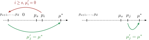
Figure 1: Illustration of the various changes of distribution considered in $\mathcal{B}(\mu)$

We consider $\tilde{\mathcal{C}}$ defined as

$$\tilde{\mathcal{C}}=\left\{(c_{i})_{i\in[d]}\in\mathbb{R}_{+}^{d}\,\middle|\,\text{for all $i\in[s]\setminus\left\{1\right\}$ and $j\in[d]\setminus[s]$},\quad\begin{aligned} &c_{i}\Delta_{i}^{2}\geqslant 1/2\\ &c_{j}\mu_{1}^{2}+c_{i}\mu_{i}^{2}\geqslant 1/2\end{aligned}\right\}$$

and we prove that $\mathcal{C}$ is a subset of $\tilde{\mathcal{C}}$, namely that there are more acceptable vectors of coefficients in $\mathcal{C}$ allowing us to reach lower values of the argument.

Let $(c_{i})_{i\in[d]}\in\mathcal{C}$ and let us prove that it belongs to $\tilde{\mathcal{C}}$. Let $i\in[s]\setminus\left\{1\right\}$, $\gamma>0$ and consider $\mu^{(i,\gamma)}\in\mathbb{R}^{d}$ defined as the following modification of $\mu$:

$$\mu_{k}^{(i,\gamma)}=\begin{cases}\mu_{1}+\gamma&\text{if $k=i$}\\ \mu_{k}&\text{otherwise},\end{cases}\quad k\in[d].$$

We easily see that $\mu^{(i,\gamma)}$ belongs to $\mathcal{B}(\mu)$. Therefore, by definition of $\mathcal{C}$, $(c_{i})_{i\in[d]}$ satisfies:

$$\sum_{k\in[d]}c_{k}(\mu_{k}-\mu_{k}^{(i,\gamma)})^{2}\geqslant\frac{1}{2},$$

which, by definition of $\mu^{(i,\gamma)}$ boils down to $c_{i}(\Delta_{i}+\gamma)^{2}\geqslant 1/2$. This being true for all $\gamma>0$, we have $c_{i}\Delta_{i}^{2}\geqslant 1/2$. The first condition in the defintion of $\tilde{\mathcal{C}}$ is then satisfied.

Similary, for $i\in[s]\setminus\left\{1\right\}$, $j\in[d]\setminus[s]$ and $\gamma>0$ we consider $\mu^{(i,j,\gamma)}\in\mathbb{R}^{d}$ defined by:

$$\mu_{k}^{(i,j,\gamma)}=\begin{cases}0&\text{if $k=i$}\\ \mu_{1}+\gamma&\text{if $k=j$}\\ \mu_{k}&\text{otherwise},\end{cases}\quad k\in[d].$$

$\mu^{(i,j,\gamma)}$ also belongs to $\mathcal{B}(\mu)$. By definition of $\mathcal{C}$, $(c_{i})_{i\in[d]}$ satisfies:

$$\sum_{k\in[d]}c_{k}(\mu_{k}-\mu_{k}^{(i,j,\gamma)})^{2}\geqslant\frac{1}{2},$$

which boils down to $c_{i}\mu_{i}^{2}+c_{j}\Delta_{j}^{2}\geqslant 1/2$ (after taking the infinimum over $\gamma>0$). Since $\Delta_{j}=\mu_{1}$, the second condition in the definition of $\tilde{\mathcal{C}}$ is satisfied. We have proved that $(c_{i})_{i\in[d]}$ belongs to $\tilde{\mathcal{C}}$ and consequently that $\mathcal{C}$ is a subset of $\tilde{\mathcal{C}}$. Therefore,

$$\liminf_{T\to+\infty}\frac{\operatorname{Reg}(T)}{\log(T)}\geqslant\inf_{c\in\mathcal{C}}\sum_{i\in[d]}c_{i}\Delta_{i}\geqslant\inf_{c\in\tilde{\mathcal{C}}}\sum_{i\in[d]}c_{i}\Delta_{i}.$$

The computation of the optimization problem over $\tilde{\mathcal{C}}$ is deferred to Appendix A. ∎

Remark 1.

This is a linear optimization problem under inequality constraints so there exist algorithmic methods such as the celebrated Simplex algorithm Dantzig (2016) to compute a numeric solution of it. Nonetheless, in our case, it is possible to give an explicit solution.

4 Sparse UCB

4.1 The SparseUCB  algorithm

The SparseUCB algorithm is formally defined in Algorithm 1 but let us first provide an informal description. The algorithm can be in different phases (denoted $\mathfrak{r},\mathfrak{f}$ and $\mathfrak{u}$), depending on past observations, and its behavior radically changes from one phase to another. At each time $t\geqslant 1$, the variable $\omega(t)\in\left\{\mathfrak{r},\mathfrak{f},\mathfrak{u}\right\}$ will specify the phase the algorithm is in. The variable is not useful for the algorithm itself, but will be handy for reference in the analysis. We now describe the different phases.

Round-robin

The algorithm starts with a round-robin phase, which corresponds to $\omega(t)=\mathfrak{r}$. Each of the $d$ arms is pulled once successively.

Then, for each time $t\geqslant d+1$, the following sets are defined:

$$\mathcal{J}(t) :=\left\{i\in[d]\,\middle|\,\overline{X}_{i}(N_{i}(t))\geqslant 2\sqrt{\frac{\log(N_{i}(t))}{N_{i}(t)}}\right\},$$

$$\mathcal{K}(t) :=\left\{i\in[d]\,\middle|\,\overline{X}_{i}(N_{i}(t))\geqslant 2\sqrt{\frac{\log(t)}{N_{i}(t)}}\right\}.$$

We will refer to the arms in $\mathcal{J}(t)$ as the active arms and those in $\mathcal{K}(t)$ as active and sufficiently sampled.

If there are less than $s$ active arms, i.e., $|\mathcal{J}(t)|<s$, the algorithm enters a round-robin phase, and pulls each arm successively. This implies that $\omega(t)=\mathfrak{r}$ for the next $d$ stages.

Force-log

If there are at least $s$ active arms, but less than $s$ sufficiently sampled arms ($|\mathcal{K}(t)|<s$), the algorithm enters a force-log phase ($\omega(t)=\mathfrak{f}$). In this phase, the algorithm pulls any arm in the set $\mathcal{J}(t)\setminus\mathcal{K}(t)$.

UCB

If the set $\mathcal{K}(t)$ contains at least $s$ arms, the algorithm enters a UCB phase ($\omega(t)=\mathfrak{u}$). The algorithm selects an arm in $\mathcal{K}(t)$ according to the UCB rule, i.e. it chooses the arm $i\in\mathcal{K}(t)$ which maximizes the quantity:

$$\overline{X}_{i}(N_{i}(t))+2\sqrt{\frac{\log(t)}{N_{i}(t)}}.$$

The pseudo-code of the whole procedure is given in Algorithm 1 and the skeleton in Figure 2.

Input: the total number of arms $d$ and the number of arms with positive means $s$

Initialization: $t\leftarrow 1$

 

for $k=1\dots d$ do /* round-robin */

       $I(t)\leftarrow k$

       ;    $\omega(t)\leftarrow\mathfrak{r}$

       ;    $t\leftarrow t+1$

       ;

end for

while $t\leqslant T$ do

       Compute $\mathcal{J}(t)\leftarrow\left\{i\in[d]\,\middle|\,\overline{X}_{i}(N_{i}(t))\geqslant 2\sqrt{\frac{\log(N_{i}(t))}{N_{i}(t)}}\right\}$

        

      Compute $\mathcal{K}(t)\leftarrow\left\{i\in[d]\,\middle|\,\overline{X}_{i}(N_{i}(t))\geqslant 2\sqrt{\frac{\log(t)}{N_{i}(t)}}\right\}$

        

       if $|\mathcal{J}(t)|<s$ then

             for $k=1\ldots d$ do /* round-robin */

                   $I(t)\leftarrow k$

                   ;    $\omega(t)\leftarrow\mathfrak{r}$

                   ;    $t\leftarrow t+1$

                   ;

             end for

            

       else if $\left|\mathcal{K}(t)\right|<s$ then /* force-log */

             $I(t)\in\mathcal{J}(t)\setminus\mathcal{K}(t)$

             ;    $\omega(t)\leftarrow\mathfrak{f}$

             ;    $t\leftarrow t+1$

             ;

       else  /* UCB */

             $I(t)\in\arg\max_{i\in\mathcal{K}(t)}\left\{\overline{X}_{i}(N_{i}(t))+2\sqrt{\frac{\log(t)}{N_{i}(t)}}\right\}$

             ;    $\omega(t)\leftarrow\mathfrak{u}$

             ;    $t\leftarrow t+1$

             ;

       end if

      

end while

Algorithm 1 SparseUCB

Figure 2: Skeleton of the SparseUCB algorithm. Each $\bullet$ corresponds to a conditional statement, where each departing arrow corresponds to a condition (which is written midway).

The broad idea is that the algorithm should quickly identify the $s$ good arms, and then pull those arms according to an UCB rule (or, alternatively, any other policy). At the end, only those $s$ good arms would be pulled an infinite number of times.

The set $\mathcal{J}(t)$ of active arms is defined in such a way that the expected number of pulls needed for a good arm to become active is finite. Therefore, only a finite number (in expectation) of round-robin phases is needed for all $s$ good arms to become active (see Lemma 7).

Reciprocally, a bad arm (with non-positive mean) is only pulled while active, that is a finite number of times in expectation. The main issue occurs when a bad arm happens to be active. In that case, the delay between two successive pulls of an active null arm typically increases exponentially fast because the regret scales with $\log(t)$. Consequently, it would take an exponential number of stages for this arm to become inactive again. And this could be dramatic for the regret if the best arm was, at the same time, inactive, as the regret would increase by a fixed constant of at least $\Delta_{2}$ on all those stages. The purpose of the force-log phases is to make sure that each active arm gets pulled sufficiently often so that the expected number of steps a bad arm remains active is finite. If the best arm happened to be inactive, then the number of active arms would drop below $s$, and performing a round-robin phase would allow it to quickly become active again.

Theorem 2.

The SparseUCB algorithm guarantees

$$\mathbb{E}\left[\operatorname{Reg}(T)\right]\lesssim\log(T)\sum_{\begin{subarray}{c}i\in[s]\\ \Delta_{i}>0\end{subarray}}\left(\frac{1}{\Delta_{i}}+\frac{\Delta_{i}}{\mu_{i}^{2}}\right),$$

where notation $\lesssim$ removes universal multiplicative constants and additive data-dependant constants. The detailed statement can be found in Appendix C.

4.2 Sketch of the proof

We decompose the event $\left\{I(t)=i\right\}$ of a good arm $i\in[s]$ being pulled at time $t\geqslant 1$ with respect to the different phases of SparseUCB:

$$\left\{I(t)=i\right\}=R_{i}(t)\sqcup F_{i}(t)\sqcup U_{i}(t)\sqcup V_{i}(t),\quad t\geqslant 1,$$ (5)

where the different events are defined as follows:

• $R_{i}(t):=\left\{I(t)=i,\ \omega(t)=\mathfrak{r}\right\}$ is event of arm $i$ being pulled at time $t$ during a round-robin phase;

• $F_{i}(t):=\left\{I(t)=i,\ \omega(t)=\mathfrak{f}\right\}$ is the event of arm $i$ being pulled at time $t$ during a force-log phase;

• $U_{i}(t):=\left\{I(t)=i,\ \omega(t)=\mathfrak{u},\ 1\in\mathcal{K}(t)\right\}$ is the event of arm $i$ being pulled at time $t$ during a UCB phase while the optimal arm is active and sufficiently sampled;

• $V_{i}(t):=\left\{I(t)=i,\ \omega(t)=\mathfrak{u},\ 1\not\in\mathcal{K}(t)\right\}$ is the event of arm $i$ being pulled at time $t$ during a UCB phase while the optimal arm is not active or not sufficiently sampled.

For the bad arms $i\in\{s+1,\ldots,d\}$, we consider a simpler decomposition. For $t\geqslant d+1$, we introduce $A_{i}(t):=\left\{I(t)=i,\ i\in\mathcal{J}(t)\right\}$, which is the event of arm $i$ being pulled at time $t$ while active, so that

$$\left\{I(t)=i\right\}=R_{i}(t)\sqcup A_{i}(t),\quad t\geqslant 1,$$

see, e.g. Property (v) from Lemma 6.

Using the above decompositions, we can write the regret as:

$$\mathbb{E}\left[\operatorname{Reg}(T)\right] =\sum_{\begin{subarray}{c}i\in[d]\\ \Delta_{i}>0\end{subarray}}\Delta_{i}\mathbb{E}\left[\sum_{t=1}^{T}\mathbbm{1}\left\{R_{i}(t)\right\}\right]+\sum_{\begin{subarray}{c}i\in[s]\\ \Delta_{i}>0\end{subarray}}\Delta_{i}\mathbb{E}\left[\sum_{t=1}^{T}\mathbbm{1}\left\{F_{i}(t)\right\}\right]+\sum_{\begin{subarray}{c}i\in[s]\\ \Delta_{i}>0\end{subarray}}\Delta_{i}\mathbb{E}\left[\sum_{t=1}^{T}\mathbbm{1}\left\{U_{i}(t)\right\}\right]$$

$$\qquad\qquad+\sum_{\begin{subarray}{c}i\in[s]\\ \Delta_{i}>0\end{subarray}}\Delta_{i}\mathbb{E}\left[\sum_{t=1}^{T}\mathbbm{1}\left\{V_{i}(t)\right\}\right]+\sum_{i=s+1}^{d}\Delta_{i}\mathbb{E}\left[\sum_{t=1}^{T}\mathbbm{1}\left\{A_{i}(t)\right\}\right].$$

We upper-bound independently the five above quantities. For the sake of clarity, we only provide here the main ideas of proof. A detailed analysis can be found in Appendix C.

Lemma 1.

The regret induced the round-robin phases is controlled by:

$$\mathbb{E}\left[\sum_{t=1}^{+\infty}\mathbbm{1}\left\{R_{i}(t)\right\}\right]\leqslant 1+3s+8\sum_{j=1}^{s}\frac{1}{\mu_{j}^{2}}\left(1+4\log\left(\frac{16}{\mu_{j}^{2}}\right)\right),\quad i\in[d].$$

Main argument of proof. The algorithm performs a round-robin phase only if less than $s$ arms are active, thus necessarily when one of the good arms $j\in[s]$ is not active. This implies that $\overline{X}_{j}(N_{j}(t))<2\sqrt{\frac{\log(N_{j}(t))}{N_{j}(t)}}$. The probability of this happening decreases exponentially fast and as a consequence, the expected number of round-robin phases is bounded. $\Box$

Lemma 2.

The regret induced by a good arm $i\in[s]$ during force-log phases is controlled by:

$$\mathbb{E}\left[\sum_{t=1}^{T}\mathbbm{1}\left\{F_{i}(t)\right\}\right]\leqslant\frac{16\log(T)+8}{\mu_{i}^{2}}.$$

Main argument of proof. Arm $i\in[s]$ is pulled during a force-log phase if its empirical mean is below $2\sqrt{\frac{\log(t)}{N_{i}(t)}}$. Because arm $i$ has a positive mean, the probability of this happening turns out to decrease exponentially, as soon as $N_{i}(t)\geqslant\frac{16\log(T)}{\mu_{i}^{2}}$. Therefore, the expected number of times arm $i$ is pulled during a force-log phase is bounded by $16\frac{\log(T)}{\mu_{i}^{2}}$ plus a constant term. $\Box$

Lemma 3.

The regret induced by a good arm $i\in[s]$ during UCB phases, while $1\in\mathcal{K}(t)$, is controlled by

$$\mathbb{E}\left[\sum_{t=1}^{T}\mathbbm{1}\left\{U_{i}(t)\right\}\right]\leqslant\frac{16\log(T)+8}{\Delta_{i}^{2}}+3.$$

Main argument of proof. The proof basically follows the steps of the classic UCB analysis by Auer et al. (2002). $\Box$

Lemma 4.

The regret induced by good arms during UCB phases, while $1\not\in\mathcal{K}(t)$, is controlled by:

$$\sum_{i\in[s]}\Delta_{i}\mathbb{E}\left[\sum_{t=1}^{T}\mathbbm{1}\left\{V_{i}(t)\right\}\right]\leqslant\frac{d\Delta_{s}\pi^{2}}{6}.$$

Main argument of proof. The algorithm performs a UCB phase if the set $\mathcal{K}(t)$ has at least $s$ arms. If it does not contain the best arm $1$, it must necessarily contain an arm $j\in\left\{s+1,\dots,d\right\}$, i.e. with nonpositive mean. As a consequence, the empirical mean of arm $j$ is above $2\sqrt{\frac{\log(t)}{N_{j}(t)}}$. Because arm $j$ has a nonpositive mean, the probability of this happening turns out to decrease as $t^{-1/2}$. Consequently, the expected number of times a good arm is pulled during a UCB phase while the best arm does not belong to $\mathcal{K}(t)$ is finite. $\Box$

Lemma 5.

The regret induced by a bad arm $i\in\left\{s+1,\dots,d\right\}$ while active is controlled by:

$$\mathbb{E}\left[\sum_{t=1}^{+\infty}\mathbbm{1}\left\{A_{i}(t)\right\}\right]\leqslant\frac{\pi^{2}}{6}.$$

Main argument of proof. Arm $i$ is active if its empirical mean is above $2\sqrt{\frac{\log(N_{i}(t))}{N_{i}(t)}}$. Because its mean is nonpositive, this happens with a total probability of the order of $\sum t^{-2}$. Therefore, the regret incurred when $i$ is active is bounded. $\Box$

It only remains to combine the above results, to upper bound the expected regret as

$$\mathbb{E}\left[\operatorname{Reg}(T)\right]\lesssim\log(T)\sum_{\begin{subarray}{c}i\in[s]\\ \Delta_{i}>0\end{subarray}}\left(\frac{1}{\Delta_{i}}+\frac{\Delta_{i}}{\mu_{i}^{2}}\right)+d\sum_{j=1}^{s}\frac{\mu_{1}\log(1/\mu_{j}^{2})}{\mu^{2}_{j}},$$

where we omitted multiplicative universal constants. We emphasize the fact that the last term is independent of $T$, hence the dominating term is

$$\mathbb{E}\left[\operatorname{Reg}(T)\right]\lesssim\log(T)\sum_{\begin{subarray}{c}i\in[s]\\ \Delta_{i}>0\end{subarray}}\max\left\{\frac{1}{\Delta_{i}},\frac{\Delta_{i}}{\mu_{i}^{2}}\right\}.$$

5 Optimality, ranges of sparsity and constants optimization

We prove in this section that the algorithm SparseUCB  is optimal, up to multiplicative factor, for a wide range of parameters. For this purpose, we recall the different bounds we obtained, up to multiplicative universal constants and additive data-dependent constants.

5.1 Strong sparsity

The regime of strong sparsity is attained when $\frac{d-s}{\mu_{1}}-\sum_{\begin{subarray}{c}i\in[s]\\ \Delta_{i}>0\end{subarray}}\frac{\Delta_{i}}{\mu_{i}^{2}}>0$. In that case, the lower bound of Theorem 1 rewrites as

$$\liminf_{T\to\infty}\frac{\operatorname{Reg}(T)}{\log(T)}\gtrsim\sum_{\begin{subarray}{c}i\in[s]\\ \Delta_{i}>0\end{subarray}}\max\Big{\{}\frac{1}{\Delta_{i}},\frac{\Delta_{i}}{\mu_{i}^{2}}\Big{\}}$$

while SparseUCB  suffers an expected regret bounded as

$$\frac{\operatorname{Reg}(T)}{\log(T)}\lesssim\sum_{\begin{subarray}{c}i\in[s]\\ \Delta_{i}>0\end{subarray}}\frac{1}{\Delta_{i}}+\frac{\Delta_{i}}{\mu_{i}^{2}}\lesssim\sum_{\begin{subarray}{c}i\in[s]\\ \Delta_{i}>0\end{subarray}}\max\Big{\{}\frac{1}{\Delta_{i}},\frac{\Delta_{i}}{\mu_{i}^{2}}\Big{\}}\ .$$

Obviously, SparseUCB  is optimal for all those values of parameters. More importantly, its regret scales linearly with $s$ and is independent of the number of arms with non-positive means.

The minimax regret of SparseUCB  is necessarily of the same order of UCB, as they achieve the same regret when $\frac{d-s}{\mu_{1}}-\sum_{\begin{subarray}{c}i\in[s]\\ \Delta_{i}>0\end{subarray}}\frac{\Delta_{i}}{\mu_{i}^{2}}$ is arbitrarily close to 0. So we consider instead the minimax regret with respect to the distributions with a relative sparsity level bounded away from 0, i.e., such that for some $\theta\in(0,1)$, $\mu_{s}\geqslant\theta\mu_{1}$. In particular, this yields that $\frac{d-s}{s}>\frac{1-\theta}{\theta^{2}}$ so that the strong sparsity assumption is satisfied.

Then, for this class of parameters, it is quite straightforward to get that the minimax regret of UCB scales as $\sqrt{dT\log(T)}\sqrt{1+\frac{\theta}{1-\theta}\frac{s}{d}}$ while the minimax regret of SparseUCB  increases as $\sqrt{sT\log(T)}\sqrt{\frac{(1-\theta)^{2}}{\theta^{2}}+1}$. As a consequence, for any fixed class of parameters, the dependency in the number of arms in the minimax regret shrinks from $\sqrt{d}$ to $\sqrt{s}$

5.2 Variants & small improvements

Of course, the minimax regret of SparseUCB exhibits an extra $\sqrt{\log(T)}$ term, which is due to the fact that we used UCB as a basic algorithm. In the order hand, we could have used instead of UCB, any variant such as UCB-2, improved-UCB, ETC, MOSS… In the same line of thoughts, the threshold of the force-log phase could also be updated to $2\sqrt{\frac{\log(T/N_{i}(t))}{N_{i}(t)}}$ so that the term $\sqrt{\log(T)}$ can be replaced by $\sqrt{\log(s)}$, which gives a regret scaling in

$$\operatorname{Reg}(T)\lesssim\left\{\begin{array}[]{ll}\sum_{\begin{subarray}{c}i\in[s]\\ \Delta_{i}>0\end{subarray}}\frac{\log(T\Delta_{i}^{2})}{\Delta_{i}}+\frac{\log(T\mu_{i}^{2})\Delta_{i}}{\mu_{i}^{2}}&\text{ in the distribution dependent sense}\\ \sqrt{sT}\sqrt{\frac{(1-\theta)^{2}}{\theta^{2}}+1}\sqrt{\log(s)+\log(\frac{(1-\theta)^{2}}{\theta^{2}}+1)}&\text{ in the minimax sense}\end{array}\right.$$

Similarly, under some additional assumptions on the probility distribution at stake, one might use KL-UCB instead of UCB to replace the dependency in $\Delta_{i}\Big{(}\frac{1}{\Delta^{2}_{i}}+\frac{\Delta_{i}}{\mu_{i}^{2}}\Big{)}$ into $\Delta_{i}\Big{(}\frac{1}{KL(\mu_{i},\mu^{*})}+\frac{\Delta_{i}}{KL(0,\mu_{i})}\Big{)}$ when this makes sense.

Another way to slightly improve the guarantees of the algorithm is to change the round-robin phases into sampling phases in which arms are not selected uniformly at random but with probability depending on the past performances of the different arms, as in Bubeck et al. (2013). Unfortunately, this does not improve the leading term (in $T$) of the regret, but merely the terms uniformly bounded (in $T$).

6 Experiments

This section aims at experimentally validating the theoretical results we obtained. We empirically compare the regret of UCB and SparseUCB for various levels of sparsity: we either fix $d$ and $s$ and allow $\mu_{s}/\Delta_{s}$ to vary or conversely fix the expected returns and allow $s/d$ to vary. According to the conclusions of Section 5, we observe that for a range of settings, SparseUCB does behave near-optimally in the long run, up to multiplicative constants. We also see that even when SparseUCB is not optimal, it is still almost always preferable to UCB as soon as there is some sparsity in the problem. Without loss of generality, experiments are performed on problems for which $\mu_{1}=0.9$ and for $2\leqslant i\leqslant s$, all $\mu_{i}$’s are equal to $\mu_{s}=\mu_{1}-\Delta_{s}$.

6.1 Varying $\mu_{s}$

We fix $d=15$ and $s=7$ such that the limit between weak and strong sparsity as defined in Section 5 is reached at $\mu_{s}=0.4$. We allow $\Delta_{s}$ to vary in $[0.1,0.7]$. We compare the behavior of SparseUCB  and UCB  for these bandit problems, and we also compute and display the lower bound of Corollary 1, that is for the smallest class of sparse of problems containing ours – for $\varepsilon=\mu_{s}$.

On Figure 3 we present the expected regret averaged over Monte-Carlo 100 repetitions for each experiment. When the sparsity of the problem is not strong, that is when $\Delta_{s}=0.7$, UCB  has a lower regret than SparseUCB for a long time but the asymptotic behavior of the latter tends to show that UCB  will eventually be worse in the long run. However, when the sparsity gets stronger, SparseUCB  is much closer to optimal than UCB  and reaches a much lower regret.

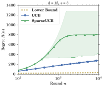
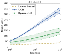
Figure 3: Cumulated regret of UCB  and SparseUCB  for $\mu^{*}=0.9$, $d=15$, $s=7$ and, from left to right, $\Delta_{s}=0.7,\,0.25,\,0.1$.

6.2 Influence of the number of arms

We now fix $d=15$, $\mu^{*}=0.9$ and $\Delta_{s}=0.3$ and we allow the number of effective arms $s$ to vary in $\{2,6,12\}$. Note that given the fixed parameters, the regime of weak sparsity defined in previous section only holds when $s>10$.

On Figure 4 we present the expected regret averaged over 100 Monte-Carlo repetitions. Clearly, when $s=12$, we are in the weak sparsity regime and there is no real improvement brought by SparseUCB  as compared to the usual UCB policy. On the contrary, as $s$ gets smaller, SparseUCB gets closer and closer to optimal.

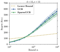
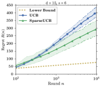
Figure 4: Cumulated regret of UCB  and SparseUCB  for $d=15$, $\mu=0.9$ and, from left to right, $s=12,6,2$.

7 Conclusions and Open Questions

We introduced a new variation of the celebrated stochastic multi-armed bandit problem that include an additional sparsity information on the expected return of the arms. We characterized the range of parameters that lead to interesting sparse problems and gave a lower bound on the regret that scales in $O(s\log(T))$ in the Strong Sparsity domain. We provide SparseUCB  that is a good alternative to the classical UCB  in the sparse bandit situation as it has both good theoretical guarantees and good empirical performances. However, we noticed in the experiments that for parameters lying in the Weak Sparsity domain, one would rather switch to the classical UCB  policy as the price of focusing on the $s$ best arms paid by SparseUCB  is too high as compared to the resulting improvement on the regret. Moreover, it appears in many real applications that the learner often knows the existence of $s$ without knowing its exact value and that leverages a new and unsolved stochastic sparse problem.

Appendix A End of Proof of Lower Bound

Recall Theorem 1:

Theorem 2.

For a Gaussian sparse bandit problem $\nu=(\nu_{1},\ldots,\nu_{s},\nu_{s+1},\ldots,\nu_{d})\in\mathcal{S}(d,s)\in\mathbb{R}^{d}$, an asymptotic lower bound on the regret is given by the solution to the following linear optimization problem:

$$f(\mu)\geqslant\quad\inf_{c\succeq 0}c_{i}\Delta_{i}$$ (6)

$$s.t. \quad\forall i\in\{2,...,s\}, 2c_{i}\Delta_{i}^{2}\geqslant 1;$$ (7)

$$\forall i\in\{2,\ldots,s\},\,\forall j\in\{s+1,...d\}, 2c_{j}\mu_{1}^{2}+2c_{i}\mu_{i}^{2}\geqslant 1$$ (8)

$$\forall i\in\{1,\ldots,d\}, c_{i}\geqslant 0$$ (9)

whose solution can be computed explicitly and gives the following problem-dependent lower bound:

• If $\frac{d-s}{\mu_{1}}-\sum_{\begin{subarray}{c}i\in[s]\\ \Delta_{i}>0\end{subarray}}\frac{\Delta_{i}}{\mu_{i}^{2}}>0$,

  $$\liminf_{T\to\infty}\frac{\operatorname{Reg}(T)}{\log(T)}\geqslant\sum_{\begin{subarray}{c}i\in[s]\\ \Delta_{i}>0\end{subarray}}\max\Big{\{}\frac{1}{2\Delta_{i}},\frac{\Delta_{i}}{2\mu_{i}^{2}}\Big{\}}$$ (10)

• otherwise, there exist $k\leqslant s$ such that $\frac{d-s}{\mu_{1}}-\sum_{i=k}^{s}\frac{\Delta_{i}}{\mu_{i}^{2}}<0$, and the lower bound is

  $$\liminf_{T\to\infty}\frac{\operatorname{Reg}(T)}{\log(T)}\geqslant\sum_{\begin{subarray}{c}i\in[k]\\ \Delta_{i}>0\end{subarray}}\frac{1}{2\Delta_{i}}+\sum_{i=k+1}^{s}\frac{\mu_{k}^{2}}{\mu_{i}^{2}}\frac{\Delta_{i}}{2\Delta_{k}^{2}}+\frac{(d-s)}{2\mu_{1}}\left(1-\frac{\mu_{k}^{2}}{\Delta_{k}^{2}}\right).$$ (11)

Proof.

We now solve the following linear programming in order to obtain the given explicit form for the Lower Bound.

$$f(\mu)\geqslant\quad\inf_{c\succeq 0}c_{i}\Delta_{i}$$

$$s.t. \quad\forall i\in\{2,...,s\}, 2c_{i}\Delta_{i}^{2}\geqslant 1;$$

$$\forall i\in\{2,\ldots,s\},\,\forall j\in\{s+1,...d\}, 2c_{j}\mu_{1}^{2}+2c_{i}\mu_{i}^{2}\geqslant 1$$

$$\forall i\in\{1,\ldots,d\}, c_{i}\geqslant 0$$

First, remark that for all the best arms $i\in\{1,\ldots,s\}$, we must have $c_{i}\geqslant 1/2\Delta_{i}^{2}$ so if $\mu_{i}^{2}/\Delta_{i}^{2}\geqslant 1$, the $d-s$ corresponding constraints on suboptimal $c_{j},j>s$ are empty. We define $S^{*}:=\left\{i\in[s]\,\middle|\,\mu_{i}^{2}/\Delta_{i}^{2}\geqslant 1\right\}$. It remains $s-|S^{*}|$ constrains on each $c_{j}$ for $j>s$:

$$c_{j}\geqslant\max_{i\in[s]\setminus S^{*}}\frac{1-2c_{i}\mu_{i}^{2}}{2\mu_{1}^{2}}=:\frac{\lambda}{2\mu_{1}^{2}}$$

It remains to properly identify $\lambda$ as a function of the parameters of the problem. Because of the first set of constraints, for all $i\notin S^{*}$,

$$c_{i}=\max\left\{\frac{1}{2\Delta_{i}^{2}},\frac{1-\lambda}{2\mu_{i}^{2}}\right\}$$

For those coefficients $i\leqslant s$ such that $c_{i}=\frac{1-\lambda}{2\mu_{i}^{2}}$, we have

$$\lambda\leqslant 1-\left(\frac{\mu_{i}}{\Delta_{i}}\right)^{2}:=\Theta_{i}\in[0,1]$$

where the quantity $\Theta_{i}$ increases with $i$, i.e. the worse the arm is, the bigger his $\Theta_{i}$. Let $k\notin S^{*}$ be the smaller index such that

$$\Theta_{k-1}<\lambda\leqslant\Theta_{k}.$$ (12)

Then, we set the values of the coefficients as

$$\begin{cases}c_{i}=1/2\Delta_{i}^{2}&i<k\\ c_{i}=(1-\lambda)/2\mu_{1}^{2}&i\geqslant k\end{cases}$$

We can rewrite the optimization problem as a function of $\lambda>\Theta_{k-1}$:

$$f(\mu)\geqslant \sum_{i=1}^{k-1}\frac{1}{2\Delta_{i}}+\sum_{i=k}^{s}\Delta_{i}\frac{1-\lambda}{2\mu_{i}^{2}}+(d-s)\frac{\lambda}{2\mu_{1}}$$

$$=\sum_{i=1}^{k-1}\frac{1}{2\Delta_{i}}+\sum_{i=k}^{s}\frac{\Delta_{i}}{2\mu_{i}^{2}}+\frac{\lambda}{2}\left(\frac{d-s}{\mu_{1}}-\sum_{i=k}^{s}\frac{\Delta_{i}}{\mu_{i}^{2}}\right)$$ (13)

Now we must distinguish two cases depending on the sign of

$$\frac{d-s}{\mu_{1}}-\sum_{i=k}^{s}\frac{\Delta_{i}}{\mu_{i}^{2}}$$ (14)

Strong sparsity.

If $\frac{d-s}{\mu_{1}}-\sum_{\begin{subarray}{c}i\in[s]\\ \Delta_{i}\geqslant 0\end{subarray}}\frac{\Delta_{i}}{\mu_{i}^{2}}>0$, then we must set the coefficients such that $\lambda$ reaches its lowest allowed value, which is $\lambda=0$. Hence, $c_{i}=\max\{\frac{1}{2\Delta_{i}^{2}},\frac{1}{2\mu_{i}^{2}}\}$ for all $i\leqslant s$. The lower bound is then

$$f(\mu)=\sum_{\begin{subarray}{c}i\in[s]\\ \Delta_{i}>0\end{subarray}}\max\Big{\{}\frac{1}{2\Delta_{i}},\frac{\Delta_{i}}{2\mu_{i}^{2}}\Big{\}}.$$

Weak sparsity

Otherwise, there exists $k\leqslant s$ such that the expression of Eq. 14 is negative. Then, we have by definition of $k$,

$$\lambda=\Theta_{k}$$

and, rearranging the terms of Eq.(13), the Lower Bound finally writes

$$\liminf_{T\to\infty}\frac{\operatorname{Reg}(T)}{\log(T)}\geqslant\sum_{i=1}^{k}\frac{1}{2\Delta_{i}}+\sum_{i=k+1}^{s}\frac{\mu_{k}^{2}}{\mu_{i}^{2}}\frac{\Delta_{i}}{2\Delta_{k}^{2}}+\frac{(d-s)}{2\mu_{1}}\left(1-\frac{\mu_{k}^{2}}{\Delta_{k}^{2}}\right).$$

A special case of the above bound is when $k=s$. Then

$$\lambda=1-\frac{\mu_{s}^{2}}{\Delta_{s}^{2}}.$$

In that case, the lower bound is

$$f(\mu)\geqslant\sum_{i=1}^{s}\frac{1}{2\Delta_{i}}+\sum_{i=s+1}^{d}\frac{\Delta_{i}(1-\mu_{s}^{2}/\Delta_{s}^{2})}{2\mu_{1}^{2}}=\sum_{i=1}^{d}\frac{1}{2\Delta_{i}}-\frac{(d-s)}{2\mu_{1}}\frac{\mu_{s}^{2}}{\Delta_{s}^{2}}$$

∎

Appendix B Generalization of Theorem 1

The lower bound of Theorem 1 can be generalized to a wider class of problems including a sparsity information. We assume that we know $\varepsilon>0$ such that $\mu_{s+1}>\mu_{s}-\varepsilon$. A sparse bandit problem as defined in Section 2 is at least included in such class of problem for $\varepsilon=\mu_{s}$. Introducing $\varepsilon>0$ allows us to provide a result that applies to our problem as well as to similar ones such as the Stochastic Thresholded Bandit for which one would assume that there exists a threshold $\mu_{s}\geqslant\tau>0$ such that the $s$ arms of interest have an expected return at of at least $\tau$. In that case, a change of variable $\varepsilon\leftarrow\mu_{s}-\tau$ in the following Theorem provides a lower bound on the regret of any uniformly efficient algorithm for that problem. We chose to introduce this wilder class of problems in order to provide a generic result and its associated proof technique, but we state the specific lower bound for our own problem in Theorem 1 below.

Theorem 3.

For a Gaussian sparse bandit problem $\nu=(\nu_{1},\ldots,\nu_{s},\nu_{s+1},\ldots,\nu_{d})\in\mathcal{S}(d,s,\varepsilon)\in\mathbb{R}^{d}$, an asymptotic lower bound on the regret is given by

• If $\frac{d-s}{\mu_{1}}-\sum_{\begin{subarray}{c}i\in[d]\\ \Delta_{i}>0\end{subarray}}\frac{\Delta_{i}}{(\mu_{i}-\mu_{s}+\varepsilon)^{2}}>0$,

  $$f(\mu)=\sum_{\begin{subarray}{c}i\in[s]\\ \Delta_{i}>0\end{subarray}}\max\Big{\{}\frac{1}{2\Delta_{i}},\frac{\Delta_{i}}{2(\mu_{i}-\mu_{s}+\varepsilon)^{2}}\Big{\}};$$

• otherwise, there exist $k\leqslant s$ such that $\frac{d-s}{\mu_{1}}-\sum_{i=k}^{s}\frac{\Delta_{i}}{(\mu_{i}-\mu_{s}+\varepsilon)^{2}}<0$, and the lower bound is

  $$\liminf_{T\to\infty}\frac{\operatorname{Reg}(T)}{\log(T)}\geqslant\sum_{i=1}^{k}\frac{1}{2\Delta_{i}}+\sum_{i=k+1}^{s}\frac{(\mu_{k}-\mu_{s}+\varepsilon)^{2}}{(\mu_{i}-\mu_{s}+\varepsilon)^{2}}\frac{\Delta_{i}}{2\Delta_{k}^{2}}+\frac{(d-s)}{2\mu_{1}}\left(1-\frac{(\mu_{k}-\mu_{s}+\varepsilon)^{2}}{\Delta_{k}^{2}}\right)..$$ (15)

Appendix C Analysis of the SparseUCB algorithm

We provide in this section the detailed statements and proofs concerning the upper bound guaranteed by the SparseUCB algorithm.

Theorem 4.

For $T\geqslant 1$, the SparseUCB algorithm guarantees:

$$\mathbb{E}\left[\operatorname{Reg}(T)\right] \leqslant 16\log(T)\sum_{\begin{subarray}{c}i\in[s]\\ \Delta_{i}>0\end{subarray}}\left(\frac{1}{\Delta_{i}}+\frac{\Delta_{i}}{\mu_{i}^{2}}\right)+\left(\sum_{i\in[d]}\Delta_{i}\right)\left(1+3s+\sum_{j=1}^{s}\frac{1+4\log(16/\mu_{j}^{2})}{\mu_{j}^{2}}\right)$$

$$\qquad\qquad\qquad+\sum_{\begin{subarray}{c}i\in[s]\\ \Delta_{i}>0\end{subarray}}\Delta_{i}\left(3+\frac{8}{\mu_{i}^{2}}+\frac{8}{\Delta_{i}^{2}}\right)+\frac{\pi^{2}}{6}\sum_{i=s+1}^{d}\Delta_{i}+\frac{d\Delta_{s}\pi^{2}}{6}.$$

We gather without proof in the following lemma a few properties which are immediate from the definition of the algorithm.

Lemma 6.

By definition of the algorithm, we have:

1. For all $t\geqslant d+1$ and $i\in[d]$, $N_{i}(t)\geqslant 1$ and the sets $\mathcal{J}(t)$ and $\mathcal{K}(t)$ are well-defined.

2. For all $t\geqslant d+1$ and $i\in[d]$, if arm $i$ is pulled at time $t$ during a round-robin phase, then the set $\mathcal{J}(t-i+1)$ contains less than $s$ arm. In other words,

   $$R_{i}(t)\subset\left\{\left|\mathcal{J}(t-i+1)\right|<s\right\}.$$

3. For all $t\geqslant 1$ and $i,k\in[d]$, arm $i$ is pulled at time $t$ during a round-robin phase if, and only if arm $k$ is also pulled during a round-robin phase at time $t-i+k$. In other words,

   $$\left\{I(t)=i,\ \omega(t)=\mathfrak{r}\right\}=\left\{I(t-i+k)=k,\ \omega(t-i+k)=\mathfrak{r}\right\}.$$

4. For all $t\geqslant d+1$ and $i\in[d]$, if arm $i$ is pulled at time $t$ during a force-log phase, it does not belong to $\mathcal{K}(t)$ i.e. its empirical mean at time $t$ is strictly below $2\sqrt{\log(t)/N_{i}(t)}$. In other words,

   $$F_{i}(t)\subset\left\{\overline{X}_{i}(N_{i}(t))<2\sqrt{\frac{\log(t)}{N_{i}(t)}},\ I(t)=i\right\}.$$

5. For all $t\geqslant 1$ and $i\in[d]$, arm $i$ is pulled at time $t$ during a force-log or a UCB phase only if it belongs to the set $\mathcal{J}(t)$. In other words, $F_{i}(t)$, $U_{i}(t)$ and $V_{i}(t)$ are subsets of $A_{i}(t)$.

6. For all $t\geqslant d+1$, if an arm is pulled at time $t$ during an UCB phase while the best arm does not belong to the set $\mathcal{K}(t)$, necessarily, a bad arm $j\in\left\{s+1,\dots,d\right\}$ belongs to $\mathcal{K}(t)$. In other words,

   $$\bigsqcup_{i\in[d]}V_{i}(t)\subset\bigcup_{j>s}\left\{\overline{X}_{j}(N_{j}(t))\geqslant 2\sqrt{\frac{\log(t)}{N_{j}(t)}}\right\}.$$

Lemma 7.

For $i\in[d]$, the number of times arm $i$ is pulled, while the algorithm is performing a round-robin phase, is bounded in expectation as:

$$\mathbb{E}\left[\sum_{t=1}^{+\infty}\mathbbm{1}\left\{R_{i}(t)\right\}\right]\leqslant 1+3s+\sum_{j=1}^{s}\frac{1}{\mu_{j}^{2}}\left(8+32\log\left(\frac{16}{\mu_{j}^{2}}\right)\right).$$

Proof.

By definition of the algorithm, arm $i$ is pulled exactly once during the first $d$ stages:

$$\sum_{t=1}^{d}\mathbbm{1}\left\{R_{i}(t)\right\}=1.$$

Let $t\geqslant d+1$. Using the definition of $R_{i}(t)$ and property (ii) from Lemma 6, we write

$$R_{i}(t)=\left\{I(t)=i,\ \omega(t)=\mathfrak{r}\right\}\cap\left\{\left|\mathcal{J}(t-i+1)\right|<s\right\}.$$

If $\left|\mathcal{J}(t-i+1)\right|<s$, necessarily, there exists $j\in[s]$ such that $j\not\in\mathcal{J}(t-i+1)$, in other words, such that:

$$\overline{X}_{j}(N_{j}(t-i+1))<2\sqrt{\frac{\log(N_{j}(t-i+1))}{N_{j}(t-i+1)}}.$$

Thus, we write:

$$R_{i}(t)\subset\bigcup_{j=1}^{s}\left\{\overline{X}_{j}(N_{j}(t-i+1))<2\sqrt{\frac{\log(N_{j}(t-i+1))}{N_{j}(t-i+1)}},\ I(t)=i,\ \omega(t)=\mathfrak{r}\right\}.$$

Therefore,

$$\sum_{t=d+1}^{+\infty}\mathbbm{1}\left\{R_{i}(t)\right\} \leqslant\sum_{j=1}^{s}\sum_{t=d+1}^{+\infty}\mathbbm{1}\left\{\overline{X}_{j}(N_{j}(t-i+1))<2\sqrt{\frac{\log(N_{j}(t-i+1))}{N_{j}(t-i+1)}},\ I(t)=i,\ \omega(t)=\mathfrak{r}\right\}$$

$$=\sum_{j=1}^{s}\sum_{\begin{subarray}{c}d<t<+\infty\\ I(t)=i\\ \omega(t)=\mathfrak{r}\end{subarray}}\mathbbm{1}\left\{\overline{X}_{j}(N_{j}(t-i+1))<2\sqrt{\frac{\log(N_{j}(t-i+1))}{N_{j}(t-i+1)}}\right\}.$$ (16)

For a given arm $j\in[s]$, the quantity $N_{j}(t-i+1)$ in the above last sum is (strictly) increasing. Indeed, let $t<t^{\prime}$ such that $I(t)=I(t^{\prime})=i$ and $\omega(t)=\omega(t^{\prime})=\mathfrak{r}$. As a consequence of property (iii) from Lemma 6, we have

1. $I(t-i+k)\neq 1$ for $k\in\left\{2,\dots,d\right\}$;

2. $I(t^{\prime}-i+1)=1$.

3. $I(t-i+j)=j$;

The above properties (i) and (ii) imply $t-i+d\leqslant t^{\prime}-i$, which in turn, together with property (iii), gives that arm $j$ is pulled at least once between time $t-i+1$ and $t^{\prime}-i$ (at time $t-i+j$). Therefore, $N_{j}(t-i+1)<N_{j}(t^{\prime}-i+1)$. Therefore, the last sum in Equation (16) can be bounded, with a change of variable, as

$$\sum_{\begin{subarray}{c}d<t<+\infty\\ I(t)=i\\ \omega(t)=\mathfrak{r}\end{subarray}}\mathbbm{1}\left\{\overline{X}_{j}(N_{j}(t-i+1))<2\sqrt{\frac{\log(N_{j}(t-i+1))}{N_{j}(t-i+1)}}\right\}\leqslant\sum_{u=1}^{+\infty}\mathbbm{1}\left\{\overline{X}_{j}(u)<2\sqrt{\frac{\log(u)}{u}}\right\}.$$

Going back to Equation (16), we can now bound the expectation of the number of times arm $i$ was pulled after time $d$ as follows:

$$\mathbb{E}\left[\sum_{t=d+1}^{+\infty}\mathbbm{1}\left\{R_{i}(t)\right\}\right] \leqslant\sum_{j=1}^{s}\sum_{u=1}^{+\infty}\mathbb{P}\left[\overline{X}_{j}(u)<2\sqrt{\frac{\log(u)}{u}}\right]$$

$$\leqslant\sum_{j=1}^{s}\sum_{u=1}^{+\infty}\mathbb{P}\left[\overline{X}_{j}(u)-\mu_{j}<2\sqrt{\frac{\log(u)}{u}}-\mu_{j}\right].$$

One can easily check that

$$u\geqslant 3+\frac{32}{\mu_{j}^{2}}\log\left(\frac{16}{\mu_{j}^{2}}\right)\quad\text{implies}\quad 2\sqrt{\frac{\log(u)}{u}}-\mu_{j}\leqslant-\frac{\mu_{j}}{2}.$$

Therefore, we set $u_{j}:=3+\lceil(32/\mu_{j}^{2})\log(16/\mu_{j}^{2})\rceil$ and write:

$$\mathbb{E}\left[\sum_{t=d+1}^{+\infty}\mathbbm{1}\left\{R_{i}(t)\right\}\right] \leqslant\sum_{j=1}^{s}\sum_{u=1}^{+\infty}\mathbb{P}\left[\overline{X}_{j}(u)-\mu_{j}<2\sqrt{\frac{\log(u)}{u}}-\mu_{j}\right]$$

$$\leqslant\sum_{j=1}^{s}\left(3+\frac{32}{\mu_{j}^{2}}\log\left(\frac{16}{\mu_{j}^{2}}\right)+\sum_{u=u_{j}}^{+\infty}\mathbb{P}\left[\overline{X}_{j}(u)-\mu_{j}<-\frac{\mu_{j}}{2}\right]\right)$$

$$\leqslant\sum_{j=1}^{s}\left(3+\frac{32}{\mu_{j}^{2}}\log\left(\frac{16}{\mu_{j}^{2}}\right)+\sum_{u=u_{j}}^{+\infty}e^{-u\mu_{j}^{2}/8}\right)$$

$$\leqslant 3s+\sum_{j=1}^{s}\frac{1}{\mu_{j}^{2}}\left(8+32\log\left(\frac{16}{\mu_{j}^{2}}\right)\right).$$

∎

Lemma 8.

For $i\in[s]$ and $T\geqslant d+1$, the number of times arm $i$ is pulled up to time $T$ during force-log phases, is bounded in expectation as:

$$\mathbb{E}\left[\sum_{t=1}^{T}\mathbbm{1}\left\{F_{i}(t)\right\}\right]\leqslant\frac{16\log(T)+8}{\mu_{i}^{2}}.$$

Proof.

Let $i\in[s]$ and $T\geqslant d+1$. By definition of the algorithm, $\mathbbm{1}\left\{F_{i}(t)\right\}=0$ for $t\leqslant d$. Using property (iv) from Lemma 6, we write

$$\sum_{t=d+1}^{T}\mathbbm{1}\left\{F_{i}(t)\right\} \leqslant\sum_{t=d+1}^{T}\mathbbm{1}\left\{\overline{X}_{i}(N_{i}(t))<2\sqrt{\frac{\log(t)}{N_{i}(t)}},\ I(t)=i\right\}$$

$$\leqslant\sum_{\begin{subarray}{c}d+1\leqslant t<+\infty\\ I(t)=i\end{subarray}}\mathbbm{1}\left\{\overline{X}_{i}(N_{i}(t))<2\sqrt{\frac{\log(T)}{N_{i}(t)}}\right\}.$$

The quantity $N_{i}(t)$ being increasing in the above sum, with a change of variable, we write:

$$\sum_{t=d+1}^{T}\mathbbm{1}\left\{F_{i}(t)\right\}\leqslant\sum_{u=1}^{+\infty}\mathbbm{1}\left\{\overline{X}_{i}(u)<2\sqrt{\frac{\log(T)}{u}}\right\}.$$

We now take the expectation:

$$\mathbb{E}\left[\sum_{t=d+1}^{T}\mathbbm{1}\left\{F_{i}(t)\right\}\right]\leqslant\sum_{u=1}^{+\infty}\mathbb{P}\left[\overline{X}_{i}(u)<2\sqrt{\frac{\log(T)}{u}}\right]=\sum_{u=1}^{+\infty}\mathbb{P}\left[\overline{X}_{i}(u)-\mu_{i}<2\sqrt{\frac{\log(T)}{u}}-\mu_{i}\right].$$

We consider $u_{0}:=\lceil 16\log(T)/\mu_{i}^{2}\rceil$ which gives that $2\sqrt{\log(T)/u}-\mu_{i}\leqslant-\mu_{i}/2$ as soon as $u\geqslant u_{0}$. Therefore,

$$\sum_{u=1}^{+\infty}\mathbb{P}\left[\overline{X}_{i}(u)-\mu_{i}<2\sqrt{\frac{\log(T)}{u}}-\mu_{i}\right] \leqslant\frac{16\log(T)}{\mu_{i}^{2}}+\sum_{u=u_{0}}^{+\infty}\mathbb{P}\left[\overline{X}_{i}(u)-\mu_{i}<-\frac{\mu_{i}}{2}\right]$$

$$\leqslant\frac{16\log(T)}{\mu_{i}^{2}}+\sum_{u=u_{0}}^{+\infty}e^{-u\mu_{i}^{2}/8}$$

$$\leqslant\frac{16\log(T)}{\mu_{i}^{2}}+\frac{8}{\mu_{i}^{2}},$$

hence the result. ∎

Lemma 9.

For $i\in[s]$ such that $\Delta_{i}>0$ and $T\geqslant 1$, we have

$$\mathbb{E}\left[\sum_{t=1}^{T}\mathbbm{1}\left\{U_{i}(t)\right\}\right]\leqslant\frac{16\log(T)+8}{\Delta_{i}^{2}}+3.$$

Proof.

Let $i\in[s]$ such that $\Delta_{i}>0$ and $t\geqslant 1$, and assume that:

$$i\in\operatorname{argmax}_{j\in\mathcal{K}(t)}\left\{\overline{X}_{j}(N_{j}(t))+2\sqrt{\frac{\log(t)}{N_{j}(t)}}\right\}\quad\text{and}\quad 1\in\mathcal{K}(t).$$

In particular, we have:

$$\overline{X}_{i}(N_{i}(t))+2\sqrt{\frac{\log(t)}{N_{i}(t)}}\geqslant\overline{X}_{1}(N_{1}(t))+2\sqrt{\frac{\log(t)}{N_{1}(t)}}.$$

Using the definition of $\Delta_{i}$, the above inequality can be equivalently written:

$$\overline{X}_{i}(N_{i}(t))-\mu_{i}\geqslant\frac{\Delta_{i}}{2}+\left(\frac{\Delta_{i}}{2}-2\sqrt{\frac{\log(t)}{N_{i}(t)}}\right)+\left(\overline{X}_{1}(N_{1}(t))-\mu_{1}+2\sqrt{\frac{\log(t)}{N_{1}(t)}}\right).$$

We consider $\tau_{i}:=\lceil 16\log(t)/\Delta_{i}^{2}\rceil$ and we can see that as soon as $N_{i}(t)\geqslant\tau_{i}$, we have:

$$\frac{\Delta_{i}}{2}-2\sqrt{\frac{\log(t)}{N_{i}(t)}}\geqslant 0.$$

When this is the case, we either have

$$\overline{X}_{i}(N_{i}(t))-\mu_{i}\geqslant\frac{\Delta_{i}}{2}\quad\text{or}\quad\overline{X}_{1}(N_{1}(t))-\mu_{1}\leqslant-2\sqrt{\frac{\log(t)}{N_{1}(t)}}.$$

With the above in mind, we can write

$$\mathbb{E}\left[\sum_{t=1}^{T}\mathbbm{1}\left\{U_{i}(t)\right\}\right] \leqslant\tau_{i}+\mathbb{E}\left[\sum_{\begin{subarray}{c}1\leqslant t\leqslant n\\ N_{i}(t)\geqslant\tau_{i}\end{subarray}}\left(\mathbbm{1}\left\{\overline{X}_{i}(N_{i}(t))-\mu_{i}\geqslant\frac{\Delta_{i}}{2}\right\}\right.\right.$$

$$\qquad\qquad\qquad\qquad\qquad\left.{}\left.{}+\mathbbm{1}\left\{\overline{X}_{1}(N_{1}(t))-\mu_{1}\leqslant-2\sqrt{\frac{\log(t)}{N_{1}(t)}}\right\}\right)\right]$$

$$\leqslant\tau_{i}+\sum_{u=\tau_{i}}^{+\infty}\mathbb{P}\left[\overline{X}_{i}(u)-\mu_{i}\geqslant\frac{\Delta_{i}}{2}\right]+\sum_{t=1}^{+\infty}\mathbb{P}\left[\overline{X}_{1}(N_{1}(t))-\mu_{1}\leqslant-2\sqrt{\frac{\log(t)}{N_{1}(t)}}\right].$$

The arms being subgaussian, we bound the above probabilities as follows:

$$\mathbb{E}\left[\sum_{t=1}^{T}\mathbbm{1}\left\{U_{i}(t)\right\}\right] \leqslant\tau_{i}+\sum_{u=\tau_{i}}^{+\infty}e^{-u\Delta_{i}^{2}/8}+\sum_{t=1}^{T}\frac{1}{t^{2}}\leqslant 1+\frac{16}{\Delta_{i}^{2}}\log(T)+\frac{8}{\Delta_{i}^{2}}+\frac{\pi^{2}}{6}$$

$$\leqslant\frac{16\log(T)+8}{\Delta_{i}^{2}}+3.$$

∎

Lemma 10.

For $T\geqslant 1$, we have

$$\sum_{i\in[s]}\Delta_{i}\mathbb{E}\left[\sum_{t=1}^{T}\mathbbm{1}\left\{V_{i}(t)\right\}\right]\leqslant\frac{d\Delta_{s}\pi^{2}}{6}.$$

Proof.

Using the fact that $\Delta_{i}\leqslant\Delta_{s}$ for all $i\in[s]$,

$$\sum_{i\in[s]}\Delta_{i}\mathbb{E}\left[\sum_{t=1}^{T}\mathbbm{1}\left\{V_{i}(t)\right\}\right]\leqslant\Delta_{s}\sum_{t=1}^{T}\mathbb{E}\left[\sum_{i\in[s]}\mathbbm{1}\left\{V_{i}(t)\right\}\right].$$

Using property (vi) from Lemma 6, we bound the above expectation as follows:

$$\mathbb{E}\left[\sum_{i\in[s]}\mathbbm{1}\left\{V_{i}(t)\right\}\right]\leqslant\sum_{j>s}\mathbb{P}\left[\overline{X}_{j}(N_{j}(t))\geqslant 2\sqrt{\frac{\log(t)}{N_{j}(t)}}\right].$$

Using the fact the arms are subgaussian and that $\mu_{j}\leqslant 0$ (for $j>s$), we bound the above probability as:

$$\mathbb{P}\left[\overline{X}_{j}(N_{j}(t))\geqslant 2\sqrt{\frac{\log(t)}{N_{j}(t)}}\right]=\mathbb{P}\left[\overline{X}_{j}(N_{j}(t))-\mu_{j}\geqslant 2\sqrt{\frac{\log(t)}{N_{j}(t)}}\right]\leqslant e^{-2\log(t)}=t^{-2}.$$

The result follows. ∎

Lemma 11.

For $i\in\left\{s+1,\dots,d\right\}$, we have

$$\mathbb{E}\left[\sum_{t=1}^{+\infty}\mathbbm{1}\left\{A_{i}(t)\right\}\right]\leqslant\frac{\pi^{2}}{6}.$$

Proof.

Let $i\in\left\{s+1,\dots,d\right\}$. By definition of the algorithm, $\mathbbm{1}\left\{A_{i}(t)\right\}=0$ for $t\leqslant d$. Using the definition of $A_{i}(t)$, we write

$$\sum_{t=1}^{+\infty}\mathbbm{1}\left\{A_{i}(t)\right\}=\sum_{t=d+1}^{+\infty}\mathbbm{1}\left\{A_{i}(t)\right\}=\sum_{\begin{subarray}{c}d<t<+\infty\\ I(t)=i\end{subarray}}\mathbbm{1}\left\{\overline{X}_{i}(N_{i}(t))\geqslant 2\sqrt{\frac{\log(N_{i}(t))}{N_{i}(t)}}\right\}.$$

In the last sum above, the quantity $N_{i}(t)$ is (strictly) incrasing. Using a change of variable, and taking the expectation, we get:

$$\mathbb{E}\left[\sum_{t=d+1}^{+\infty}\mathbbm{1}\left\{A_{i}(t)\right\}\right]\leqslant\mathbb{E}\left[\sum_{u=1}^{+\infty}\mathbbm{1}\left\{\overline{X}_{i}(u)\geqslant 2\sqrt{\frac{\log(u)}{u}}\right\}\right]=\sum_{u=1}^{+\infty}\mathbb{P}\left[\overline{X}_{i}(u)\geqslant 2\sqrt{\frac{\log(u)}{u}}\right].$$

We now use the assumption that the arms have subgaussian laws and that $\mu_{i}\leqslant 0$ to bound the above probability as:

$$\mathbb{P}\left[\overline{X}_{i}(u)\geqslant 2\sqrt{\frac{\log(u)}{u}}\right]\leqslant\mathbb{P}\left[\overline{X}_{i}(u)-\mu_{i}\geqslant 2\sqrt{\frac{\log(u)}{u}}\right]\leqslant e^{-2\log(u)}=u^{-2}.$$

The result follows. ∎

References

- Abbasi-Yadkori et al. (2012) Yasin Abbasi-Yadkori, David Pal, and Csaba Szepesvari. Online-to-confidence-set conversions and application to sparse stochastic bandits. In AISTATS, volume 22, pages 1–9, 2012.
- Auer et al. (2002) Peter Auer, Nicolo Cesa-Bianchi, and Paul Fischer. Finite-time analysis of the multiarmed bandit problem. Machine learning, 47(2-3):235–256, 2002.
- Bubeck and Cesa-Bianchi (2012) Sébastien Bubeck and Nicolo Cesa-Bianchi. Regret analysis of stochastic and nonstochastic multi-armed bandit problems. arXiv preprint arXiv:1204.5721, 2012.
- Bubeck et al. (2013) Sébastien Bubeck, Vianney Perchet, and Philippe Rigollet. Bounded regret in stochastic multi-armed bandits. In COLT, pages 122–134, 2013.
- Burnetas and Katehakis (1996) Apostolos N Burnetas and Michaël N Katehakis. Optimal adaptive policies for sequential allocation problems. Advances in Applied Mathematics, 17(2):122–142, 1996.
- Carpentier et al. (2012) Alexandra Carpentier, Rémi Munos, et al. Bandit theory meets compressed sensing for high dimensional stochastic linear bandit. In AISTATS, pages 190–198, 2012.
- Cesa-Bianchi and Lugosi (2006) Nicolo Cesa-Bianchi and Gábor Lugosi. Prediction, learning, and games. Cambridge university press, 2006.
- Combes et al. (2015) Richard Combes, Mohammad Sadegh Talebi Mazraeh Shahi, Alexandre Proutiere, et al. Combinatorial bandits revisited. In Advances in Neural Information Processing Systems, pages 2116–2124, 2015.
- Dantzig (2016) George Dantzig. Linear programming and extensions. Princeton university press, 2016.
- Garivier et al. (2017.To appear.) Aurélien Garivier, Pierre Ménard, and Gilles Stoltz. Explore first, exploit next: The true shape of regret in bandit problems. Mathematics of Operations Research, 2017.To appear.
- Gerchinovitz (2013) Sébastien Gerchinovitz. Sparsity regret bounds for individual sequences in online linear regression. Journal of Machine Learning Research, 14(Mar):729–769, 2013.
- Graves and Lai (1997) Todd L Graves and Tze Leung Lai. Asymptotically efficient adaptive choice of control laws in controlled markov chains. SIAM journal on control and optimization, 35(3):715–743, 1997.
- Kaufmann et al. (2015) Émilie Kaufmann, Olivier Cappé, and Aurélien Garivier. On the complexity of best arm identification in multi-armed bandit models. Journal of Machine Learning Research, 2015.
- Kwon and Perchet (2016) Joon Kwon and Vianney Perchet. Gains and losses are fundamentally different in regret minimization: the sparse case. Journal of Machine Learning Research, 17(229):1–32, 2016.
- Lagrée et al. (2016) Paul Lagrée, Claire Vernade, and Olivier Cappé. Multiple-play bandits in the position-based model. arXiv preprint arXiv:1606.02448, 2016.
- Lai and Robbins (1985) Tze Leung Lai and Herbert Robbins. Asymptotically efficient adaptive allocation rules. Advances in applied mathematics, 6(1):4–22, 1985.
- Langford et al. (2009) John Langford, Lihong Li, and Tong Zhang. Sparse online learning via truncated gradient. Journal of Machine Learning Research, 10(Mar):777–801, 2009.
- Lattimore et al. (2015) Tor Lattimore, Koby Crammer, and Csaba Szepesvári. Linear multi-resource allocation with semi-bandit feedback. In Advances in Neural Information Processing Systems, pages 964–972, 2015.
- Robbins (1985) Herbert Robbins. Some aspects of the sequential design of experiments. In Herbert Robbins Selected Papers, pages 169–177. Springer, 1985.