Miscible-Immiscible Transition and Nonequilibrium Scaling in Two-Component Driven Open Condensate Wires

Abstract

We investigate the steady state phase diagram of two-component driven open condensates in one dimension. We identify a miscible-immiscible transition which is predominantly driven by gapped density fluctuations and occurs upon increasing the inter-component dissipative coupling. Below the transition in the miscible phase, we find the effective long wavelength dynamics to be described by a two-component Kardar-Parisi-Zhang (KPZ) equation that belongs to the nonequilibrium universality class of the one-dimensional single-component KPZ equation at generic choices of parameters. Our results are relevant for different experimental realizations for two-component driven open condensates in exciton-polariton systems.

1 Introduction

Recent experimental development in nanoscience, quantum optics, ultracold atom physics and related areas has given rise to new classes of synthetic physical systems with properties of both fundamental and practical interests. One class of these systems are quantum many body ensembles in a driven open setting, which includes exciton-polaritons in semiconductor heterostructures [1, 2, 3, 4, 5, 6, 7, 8, 9], ultracold atoms [10, 11, 12], trapped ions [13, 14], and microcavity arrays [15, 16]. The unifying and characteristic trait of these systems is the breaking of detailed balance on the microscopic level, making them promising laboratories to advance the frontier of nonequilibrium statistical physics.

One current research focus are driven open condensates (DOCs). They can be realized, for instance, in exciton-polariton systems [1, 2, 3, 4, 5, 6, 7, 8, 9]. On the one hand, recent theoretical investigations [17, 18, 19, 20, 21, 22, 23, 24] on single-component DOCs have revealed a new class of nonequilibrium phenomena, that are related to a variant of the famous Kardar-Parisi-Zhang (KPZ) equation [25] in nonequilibrium statistical physics. On the other hand, investigations on multi-component Bose-Einstein condensates (BECs), realized mainly in ultracold atom experiments, have shown that the inter-component couplings generally give rise to very rich physics [26, and the references therein]. For instance, in the simplest case, i.e., two-component BECs, it is well known that a strong enough inter-component interaction drives a miscible-immiscible transition, also called phase separation, via fluctuations of sound mode type [27, 28, 29, 30], and where, in the phase separation the two components avoid each other spatially. Its existence can thus be traced back to the closed nature of these systems, namely, to the simultaneous presence of both particle number and momentum conservation. These are ingredients that are explicitly violated in their driven-open counterparts. Such a setting therefore gives rise to a novel scenario for the miscible-immiscible transition, and, more generally, for the physical effects of inter-component couplings in multi-component condensates in a generic driven-open setup. In light of recent developments realizing multicomponent DOCs via different polarization degrees of freedom [7, 8, 9] or polaritonic Feshbach resonances [6], understanding the generic features of the phase diagram of such systems becomes a pressing task.

As a first step to address questions along this line, we investigate one-dimensional (1D) two-component DOCs at relatively weak noise strength and under weak nonequilibrium condition in this work, with particular focus on the physical effects of the inter-component couplings. To this end, we establish the phase diagram of the system in terms of the dimensionless inter-component coherent coupling (elastic two-body collisions) $\tilde{v}_{c}\equiv v_{c}/\sqrt{u_{1,c}u_{2,c}}$ and dissipative coupling (two-body losses) $\tilde{v}_{d}\equiv v_{d}/\sqrt{u_{1,d}u_{2,d}}$ as shown in Fig. 1(a), where $v_{c}$ and $v_{d}$ are the coherent and dissipative inter-component couplings, respectively; $u_{j,c}$ and $u_{j,d}$ are the intra-component elastic collision strength and positive two-particle loss rate, respectively, with $j=1,2$ being the component index. More specifically, we find: (i) A miscible-immiscible transition at finite $\tilde{v}_{d}$. Interestingly, the mechanism behind that transition is different depending on the regime of $\tilde{v}_{d}$. For $\tilde{v}_{d}>1$, the transition is driven by $\tilde{v}_{d}$ itself via the gapped density fluctuations [cf. Fig. 1(a) and Eq. (12)]. We notice that this condition $\tilde{v}_{d}>1$ interestingly shares a form analogous to the one in the purely coherent two-component BEC, i.e., $\tilde{v}_{c}>1$ [30]. The mechanism underlying the transition is however vastly different, since in purely coherent two-component BECs, the transition is driven by the gapless sound modes [30]. For $\tilde{v}_{d}<1$, the transition is driven by the inter-component coherent coupling $\tilde{v}_{c}$ via gapless diffusive modes [cf. Eq. (13)], whose critical value can be strongly affected by the presence of dissipative couplings in the system [cf. Fig. 1(a), Eqs. (16), (17)]. The clearest signatures of the immiscible state is present in single experimental runs, where the two components avoid each other spatially (ii) Below the transition in the miscible phase, we find that the long wavelength dynamical behavior of the system is effectively described by a two-component KPZ equation, where, in particular, the KPZ-nonlinearity of one component is coupled to the dynamics of the other one [cf. Eq. (18)]. We further show that this two-component KPZ equation, and hence also the dynamical behavior of two-component DOCs, belongs to the nonequilibrium dynamical universality class of the 1D single-component KPZ equation at generic choices of parameters [cf. Figs. 1(c1, c2)]. In other words, at generic choices of parameters, the inter-component coupling is irrelevant in the renormalization group (RG) sense in the miscible phase, highlighting the remarkable degree of universality of KPZ physics.

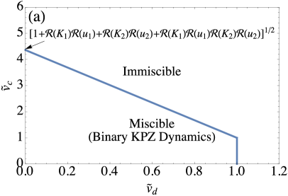
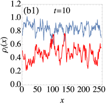
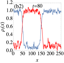
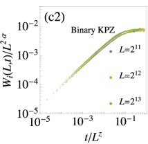
Figure 1: (a) Phase diagram of the system in terms of the rescaled dimensionless inter-component coherent coupling $\tilde{\upsilon}_{c}$ and the dissipative one $\tilde{\upsilon}_{d}$ at weak noise level and under weak nonequilibrium condition. Function $\mathcal{R}(z)\equiv\Re(z)/\Im(z)$ for $z\in\mathbb{C}$. The values of other parameters used in the phase digram are $r_{1,d}=u_{1,d}=K_{1,d}=1$, $r_{1,c}=u_{1,c}=0.1$, $K_{1,c}=3.0$; $r_{2,d}=u_{2,d}=1.1,\,K_{2,d}=1.05$, $r_{2,c}=u_{2,c}=0.11$, $K_{2,c}=3.1$. (b1, b2) Snapshots of distributions of condensate field amplitudes $\rho_{j}(x)\equiv|\psi_{j}(x)|$ in the immiscible phase at different time (the blue and red curve correspond to $\rho_{1}(x)$ and $\rho_{2}(x)$, respectively), where an immiscible phase is clearly observed at a sufficiently long time ($t=80$). The values of other parameters are $\sigma_{i}=0.01$, $v_{d}=1.2$, $v_{c}=0.05$. (c1, c2) Finite size critical scaling collapse for the roughness function $W_{j}(L,t)$ for the two-component DOC in the miscible phase (c1) and for the two-component KPZ equation Eq. (18) (c2). For the two-component DOC, the value of other parameters are $\sigma_{1}=0.04,\sigma_{2}=0.05$, $v_{d}=0.6$, $v_{c}=0.2$. For the two-component KPZ equation, the parameters are $(D_{11},D_{12},D_{21},D_{22})=(1,0.5,0.55,1.1)$, $(\lambda_{11},\lambda_{12},\lambda_{21}\lambda_{22})=(7,2,2.5,7.5)$, $(\sigma_{1}^{\mathrm{KPZ}},\sigma_{2}^{\mathrm{KPZ}})=\left(0.1,0.11\right)$. The lower and upper set of curves in each plot correspond to $W_{1}(L,t)$ and $W_{2}(L,t)$, respectively. The critical exponents of the 1D single-component KPZ equation $z=3/2,\,\alpha=1/2$ yield a good finite size data scaling collapse shown in (c1, c2), which suggests that the dynamics of two-component DOC in the miscible phase and the two-component KPZ equation belong to the same dynamical universality class of the 1D single-component KPZ equation at generic choices of parameters. See text for more details.

2 Microscopic model

We describe the dynamics of the two-component 1D DOC by a generic minimal model that assumes the form of a two-component version of the stochastic complex Ginzburg-Landau equation (SCGLE) as appropriate for the exciton-polariton systems [8, 9, 17, 31, 32, 33, 34], which reads (units $\hbar=1$)

$$\partial_{t}\psi_{j}=\left(K_{j}\partial_{x}^{2}+r_{j}-u_{j}|\psi_{j}|^{2}-v|\psi_{\bar{j}}|^{2}\right)\psi_{j}+\zeta_{j},$$ (1)

with indices $j,\bar{j}=1,2$ and $\bar{j}\neq j$, denoting different components. In exciton-polariton systems, they correspond to the two polarization directions of polaritons [6, 7]. Here $K_{j}=K_{j,d}+iK_{j,c}$, $r_{j}=r_{j,d}+ir_{j,c}$, $u_{j}=u_{j,d}+iu_{j,c}$, $v=v_{d}+iv_{c}$, $\langle\zeta_{j}^{*}(x,t)\zeta_{j^{\prime}}(x^{\prime},t^{\prime})\rangle=2\sigma_{j}\delta_{jj^{\prime}}\delta(x-x^{\prime})\delta(t-t^{\prime})$ and $\langle\zeta_{j}(x,t)\zeta_{j^{\prime}}(x^{\prime},t^{\prime})\rangle=0$, where $K_{j,c}=1/m_{\mathrm{LP}}$ with $m_{\mathrm{LP}}$ being the effective polariton mass in exciton-polariton systems, and $K_{j,d}$ is a diffusion constant. $r_{j,c}$ simply reflects the choice of the rotating frame and can be modified by changing to a different frame, i.e., $\psi_{j}(x,t)=\psi_{j}^{\prime}(x,t)e^{i\mu_{j}t}$, with modified $r_{j,c}^{\prime}=r_{j,c}+\mu_{j}$. $u_{j,c}$ is the elastic collision strength. $r_{j,d}=\gamma_{j,p}-\gamma_{j,l}$ is the difference between the single particle pump and loss, denoted by $\gamma_{j,p}$ and $\gamma_{j,l}$, respectively. For the existence of condensates in the mean field steady state solution, $r_{j,d}$ has to be positive, i.e., the single-particle pump rate has to be larger than the loss rate. $u_{j,d}$ is the positive two-particle loss rate. $v_{c}$ and $v_{d}$ are the coherent (elastic) and dissipative inter-component couplings, respectively. Both of them are assumed to be positive in the following, indicating a positive inter-component elastic collision strength and positive inter-component two-particle loss rate. In exciton-polariton systems, $u_{j,d}$ and $v_{d}$ originate from intra-component and inter-component gain-saturation nonlinearities [8], respectively, instead of additional loss mechanisms. Consequently the noise strength $\sigma_{j}$ is set by the single particle loss $\gamma_{j,l}$, i.e., $\sigma_{j}=\gamma_{j,l}$ (cf. [17] for a related discussion in the single component case). We obtain most of the numerical results presented in this work by directly solving Eq. (1) using the same numerical approach as in Ref. [20] and set $r_{1,d}=K_{1,d}=1$, indicating $t$ and $x$ are measured in units of $r_{1,d}^{-1}$ and $\sqrt{K_{1,d}}$, respectively. For performing the ensemble average, we use $10^{3}$ stochastic trajectories if not mentioned otherwise.

3 Miscible-immiscible transition

In the context of ultracold atom physics, it is well known that in multi-component BEC systems, large enough inter-component interactions can drive various miscible-immiscible transitions [27, 28, 29, 30, 35, 36, 37]. In particular, in two-component BECs, if the inter-component interaction $v_{c}>\sqrt{u_{1,c}u_{2,c}}$, it can drive a transition from a miscible phase to an immiscible phase or phase separation [27, 28, 29, 30], where particles of different components stay away from each other in space. The dynamical reason that drives this transition comes from the instability caused by fluctuations of the sound mode type [30], whose existence relies on the condition that both the particle number and the momentum conservation are present. However, for two-component DOCs, this condition is apparently absent due to the driven-open characteristic of the system. More interestingly, the inter-component dissipative coupling $v_{d}$ is clearly a new relevant coupling in two-component DOCs that could be important in the miscible-immiscible transition. In the following, we shall investigate the key factors that determine the miscible-immiscible transition in this driven-open case and identify the dynamical modes that are responsible for that transition.

To this end, we perform a leading order stability analysis on the system’s deterministic dynamics, where we choose $r_{j,c}$ in such a way that, in the absence of noise, the equation of motion (EOM) Eq. (1) has a stationary, spatially uniform solution, and linearize the system’s deterministic dynamics around this solution. We denote the stationary, spatially uniform solution as $\psi_{j}^{(0)}(x,t)$, whose explicit form reads $\psi_{j}^{(0)}(x,t)=M_{j},$ with $M_{j}$ being the amplitude of $\psi_{j}^{(0)}$ that solves the homogenous real part of Eq. (1) with the explicit form $M_{j}^{2}=(r_{j,d}u_{\bar{j},d}-r_{\bar{j},d}v_{d})/(u_{1,d}u_{2,d}-v_{d}^{2})$. In general, $\psi_{j}$ can be expressed as the sum of $\psi_{j}^{(0)}$ and fluctuations $\delta\psi_{j}$ on its top, i.e., $\psi_{j}=\psi_{j}^{(0)}+\delta\psi_{j}$, where fluctuation fields $\delta\psi_{j}$ can be further decomposed into their Fourier components, i.e., $\delta\psi_{j}(x,t)=\sum_{k}c_{j,k}(t)\exp(ikx)$, with $c_{j,k}(t)$ being fluctuation amplitudes, whose two independent linear combinations, $\delta\rho_{j,k}(t)\equiv\psi_{j}^{(0)*}c_{j,k}(t)+\mathrm{c.c.}$ and $\delta\Theta_{j,k}(t)\equiv(\psi_{j}^{(0)*}c_{j,k}(t)-\mathrm{c.c.})/i$, are related to density and phase fluctuations, respectively. From the deterministic part of Eq. (1), we can directly get the EOM for $\delta\rho_{j,k}(t)$ and $\delta\Theta_{j,k}(t)$ up to their leading order, whose explicit forms read

$$\partial_{t}\left(\begin{array}[]{c}\delta\rho_{1,k}\\ \delta\Theta_{1,k}\\ \delta\rho_{2,k}\\ \delta\Theta_{2,k}\end{array}\right)=\Xi\left(\begin{array}[]{c}\delta\rho_{1,k}\\ \delta\Theta_{1,k}\\ \delta\rho_{2,k}\\ \delta\Theta_{2,k}\end{array}\right),$$ (2)

where $\Xi$ is a $4\times 4$ matrix with the explicit form

$$\Xi=\left(\begin{array}[]{cc}\Xi_{11}&\Xi_{12}\\ \Xi_{21}&\Xi_{22}\end{array}\right),\,\Xi_{j\bar{j}}\equiv-2M_{j}^{2}\left(\begin{array}[]{cc}v_{d}&0\\ v_{c}&0\end{array}\right),$$ (7)

$$\Xi_{jj}\equiv\left(\begin{array}[]{cc}-K_{j,d}k^{2}-2M_{j}^{2}u_{j,d}&K_{j,c}k^{2}\\ -K_{j,c}k^{2}-2M_{j}^{2}u_{j,c}&-K_{j,d}k^{2}\end{array}\right).$$ (10)

Plugging the resolution

$$\delta\rho_{i,k}(t)=\delta\tilde{\rho}_{i,k}e^{\omega t},\,\delta\Theta_{i,k}(t)=\delta\tilde{\Theta}_{i,k}e^{\omega t},$$ (11)

into the EOM (2), we get a set of linear equations for $\delta\tilde{\rho}_{i,k}$ and $\delta\tilde{\Theta}_{i,k}$, i.e., $\omega\mathbf{v}=\Xi\cdot\mathbf{v}$ with $\mathbf{v}\equiv(\delta\tilde{\rho}_{1,k},\delta\tilde{\Theta}_{1,k},\delta\tilde{\rho}_{2,k},\delta\tilde{\Theta}_{2,k})^{T}$, from which we can get the dispersion relations $\omega_{a,k}$ with $a=1,2,3,4,$ for the four eigenmodes of the fluctuations. The expressions for $\omega_{a,k}$ can be obtained analytically, whose forms to the leading order in momentum $k$ read

$$\omega_{a,k}=\omega_{a}^{(0)}-k^{2}\frac{\mathcal{C}_{1}+\mathcal{C}_{2}\omega_{a}^{(0)}+\mathcal{C}_{2}(\omega_{a}^{(0)})^{2}}{(\omega_{a}^{(0)})^{2}-\omega_{1}^{(0)}\omega_{3}^{(0)}},\,\mathrm{for}\,a=1,3,$$ (12)

$$\omega_{a,k}=-k^{2}\frac{\mathcal{C}_{1}\pm\sqrt{\mathcal{C}_{1}^{2}-4\mathcal{C}_{0}\omega_{1}^{(0)}\omega_{3}^{(0)}}}{2\omega_{1}^{(0)}\omega_{3}^{(0)}},\,\mathrm{for}\,a=2,4,$$ (13)

where $\omega_{a}^{(0)}$ is the zero momentum part of $\omega_{a,k}$ with the explicit forms $\omega_{2,4}^{(0)}=0$ and

$$\omega_{1,3}^{(0)} = -M_{1}^{2}u_{1,d}-M_{2}^{2}u_{2,d}\mp\sqrt{\left(M_{1}^{2}u_{1,d}-M_{2}^{2}u_{2,d}\right)^{2}+4M_{1}^{2}M_{2}^{2}v_{d}^{2}}.$$ (14)

Here, $\mathcal{C}_{0},\mathcal{C}_{1},\mathcal{C}_{2}$ are polynomials of $M_{j},K_{j,\kappa}u_{j,\kappa},v_{\kappa}$ with $\kappa=c,d$, whose explicit forms are presented in A. We can see that $\omega_{1,k}$ and $\omega_{3,k}$ are associated to density fluctuations which are gapped (finite damping rate as $k\to 0$), and $\omega_{2,k}$, $\omega_{4,k}$ are associated to phase fluctuations which are gapless diffusive modes. This phenomenology is due to the absence of particle number conservation, and is in sharp contrast to the case of the purely coherent two-component BEC, where all the low frequency fluctuations are gapless sound modes with linear dispersion relations [30].

From the form of the resolution in Eq. (11) for the fluctuations, we can see that in order for the miscible solution $\psi_{j}^{(0)}(x,t)$ to be stable, $\omega_{a,k}<0$ is required. At zeroth order in momentum, this requires that $\omega_{1,3}^{(0)}<0$, which gives rise to the condition

$$\tilde{v}_{d}<1,$$ (15)

with $\tilde{v}_{d}\equiv v_{d}/\sqrt{u_{1,d}u_{2,d}}$ being the rescaled dimensionless inter-component dissipative coupling, indicating that a large enough $v_{d}$ can drive a transition to the immiscible phase via exponentially growing gapped density fluctuations in the homogeneous state, rendering it unstable.

When the condition (15) is satisfied, requiring $\omega_{a,k}<0$ indicates the dispersion relations for the two diffusive mode $\omega_{2,k}$, $\omega_{4,k}$ should be both negative at the leading order in momentum, which gives rise to the condition

$$\mathcal{C}_{1}>0\,\mathrm{and}\,\mathcal{C}_{0}>0,$$ (16)

whose explicit form in terms of $K_{j,\kappa},u_{j,\kappa},v_{\kappa}$ can be found in appendix A. When $v_{d}=0$, the condition (16) reads

$$\tilde{v}_{c} < \left[1+\mathcal{R}(K_{1})\mathcal{R}(u_{1})+\mathcal{R}(K_{2})\mathcal{R}(u_{2})+\mathcal{R}(K_{1})\mathcal{R}(u_{1})\mathcal{R}(K_{2})\mathcal{R}(u_{2})\right]^{1/2},$$ (17)

where $\tilde{v}_{c}\equiv v_{c}/\sqrt{u_{1,c}u_{2,c}}$ is the rescaled dimensionless inter-component coherent coupling strength and function $\mathcal{R}(z)\equiv\Re(z)/\Im(z)$ for $z\in\mathbb{C}$. This is to be compared to the related condition in the purely coherent BEC case, where $\tilde{v}_{c}<1$ is required to avoid the transition to the immiscible phase [30], indicating that particularly in the absence of a dissipative inter-component dissipative coupling $v_{d}$, the two-component DOCs are generally more stable against the gapless (diffusive) fluctuations.

Requiring both the gapped density fluctuations and the diffusive phase fluctuations to decay exponentially with respect to time, i.e., both condition (15) and (16) are satisfied, gives rise to the miscible-immiscible transition boundary of the system [cf. Fig. 1(a) for the boundary in terms of $\tilde{v}_{c}$ and $\tilde{v}_{d}$ at a particular choice of other parameters]. Indeed, we observe in numerical simulations that once $(\tilde{v}_{d},\tilde{v}_{c})$ is tuned outside the miscible-immiscible transition boundary, despite being initialized with a generic homogeneous configuration in the miscible phase, the system quickly evolves into an immiscible phase, where different components occupy different spatial regions [cf. Figs. 1(b1) and (b2)].

The stability analysis presented above is independent of dimension, and we thus expect the miscible-immiscible transition to be present in any dimension. Moreover, we expect this transition behavior persists to finite noise levels. Fig. 1(b2) shows a snapshot of the system for a single stochastic trajectory, where an immiscible phase or a phase separation can be clearly identified. However, the phase separation behavior is not expected to show in the trajectory ensemble averaged density distribution in one dimension, since the locations of the phase separated regions in different stochastic trajectories are random and the interfaces between the domains are pointlike. As an ensemble average signature of the immiscible phase, one may expect exponential scaling of the temporal correlation function beyond the scale set by the typical size of phase separated regions, cutting off the subexponential diffusive or KPZ scaling expected at weak noise level and nonequilibrium strength (to be discussed in the following section). Moreover, position resolved density-density correlation function between different components should also reveal the signature of the immiscible phase.

4 Long wavelength properties of the two-component DOC in the miscible phase

Now let us discuss the long wavelength properties of the system. We have seen from the previous section that there are two phases in the system, namely, miscible and immiscible phase. In the immiscible phase, the different components occupy different spatial regions. Due to the fact that all the couplings in the system are local, one naturally expects that the two-component DOC system reduces to two independent single-component ones with the properties revealed in previous investigations [17, 18, 19, 20, 22, 23, 24].

Therefore, in the following discussion, we shall only focus on the long wavelength properties of the miscible phase. To this end, we first derive a low frequency effective description of the system’s dynamics in the miscible phase, and then investigate the long wavelength scaling behavior of the system by studying the condensate phase roughness and fluctuation functions as specified below.

4.1 Low frequency effective description of the miscible phase

For the single-component DOC, in the absence of phase defects, the low frequency dynamics is effectively described by the single-component KPZ equation [25] for the phase of the condensate field [17]. Following the lines of the derivation presented in  [17], we obtain an effective description for the low frequency dynamics for the two-component DOC, and find it assumes the form of a two-component KPZ equation with inter-component couplings which reads

$$\partial_{t}\theta_{j}=\sum_{j^{\prime}=1,2}\left[D_{jj^{\prime}}\partial_{x}^{2}\theta_{j^{\prime}}+\lambda_{jj^{\prime}}\left(\partial_{x}\theta_{j^{\prime}}\right)^{2}\right]+\xi_{j},\,j=1,2,$$ (18)

where $D_{jj^{\prime}},\,\lambda_{jj^{\prime}},\,\sigma_{j}^{\mathrm{KPZ}}$ are rational functions of $K_{j,\kappa},r_{j,\kappa},u_{j,\kappa},v_{\kappa}$$,\sigma_{j}$, whose explicit forms and derivation details are presented in appendix B. Here, $D_{jj^{\prime}}$ characterizes phase diffusion, $\xi_{j}$ is a Gaussian white noise field of strength $2\sigma_{j}^{\mathrm{KPZ}}$, i.e., $\langle\xi_{j}(x,t)\xi_{j^{\prime}}(x^{\prime},t^{\prime})\rangle=2\sigma_{j}^{\mathrm{KPZ}}\delta_{jj^{\prime}}\delta(x-x^{\prime})\delta(t-t^{\prime})$. The nonlinearities $\lambda_{jj^{\prime}}$ characterize the system’s deviation from thermodynamic equilibrium. Indeed, from the explicit form of $\lambda_{jj^{\prime}}$ presented in appendix B, we can see that all the nonlinearities $\lambda_{jj^{\prime}}$ vanish identically under detailed balance conditions, i.e., $\mathcal{R}(K_{j})=\mathcal{R}(r_{j})=\mathcal{R}(u_{j})=\mathcal{R}(v)$, which is similar to the single-component DOC case  [17].

We remark here that the effective description (18) is built on the assumption that the compactness of the phase fields can be neglected. As has been shown in related investigations in 1D single component DOCs [24], this assumption is a good approximation at low noise level and under weak nonequilibrium condition. However, it breaks down at high noise levels or under strong nonequilibrium conditions, where the compactness of the phase fields is expected to strongly influence the physics of the system and, therefore, has to be taken into account carefully. In these cases, we expect the low frequency effective description should assume the form of a compact version of equation (18), similar to what has been shown in the single-component DOC [24]. We leave the study of the system at high noise level, or under strong nonequilibrium condition, to a future investigation.

4.2 Scaling behavior of roughness function for two-component KPZ equation and DOC

Since the long wavelength dynamics of the system is effectively described by the two-component KPZ equation (18), let us first investigate its long wavelength scaling properties. To this end, we investigate the so-called “roughness function” $W_{j}(L,t)$ of the two-component KPZ equation, which is defined as $W_{j}(L,t)\equiv\langle L^{-1}\int_{x}\theta_{j}^{2}(x,t)-\left[L^{-1}\int_{x}\theta_{j}(x,t)\right]^{2}\rangle$ and measures the spatial averaged fluctuation of $\theta_{j}(x,t)$ at time $t$ of a finite system with the linear size $L$ under periodic boundary conditions. The importance of the roughness function $W_{j}(L,t)$ lies in the fact that its scaling behavior with respect to $L$ and $t$ reveals the static and dynamical critical exponents of the system, denoted as $\alpha$ and $z$, respectively. We remark here that in order to use the roughness function as a tool to reveal the universality class of the dynamics, the phase roughness of initial states should be considerably smaller than the saturation value of the roughness function at the corresponding fixed system size. In the context of exciton-polariton condensates, this type of initial condition could possibly be achieved by imposing an additional resonant laser that depresses the spatial phase fluctuations of the condensate.

In Fig. 1(c2), we show the roughness function $W_{j}(L,t)$ for the two-component KPZ equation (18) at a generic set of parameters in the scaling axes using the critical exponents of the 1D single-component KPZ equation, i.e., $z=3/2,\,\alpha=1/2$ [25, 38]. We notice good finite size critical scaling collapses for both $W_{1}(L,t)$ and $W_{2}(L,t)$. This suggests that at generic choices of parameters, the two-component KPZ equation belongs to the dynamical universality class of the 1D single-component KPZ equation.

From the scaling behavior of the two-component KPZ equation shown in the above discussion, we naturally expect the low frequency dynamics of the two-component DOC [described by the full SCGLE Eq. (1)] at generic choice of parameters should also belong to the dynamical universality class of the 1D single-component KPZ equation. Indeed, as we can see from Fig. 1(c1), the phase roughness functions $W_{j}(L,t)$s for the two-component DOC indeed show good finite size critical scaling collapses by employing the critical exponents of the 1D single-component KPZ equation.

We remark here that other forms of 1D two-component KPZ equations also emerge in different contexts in nonequilibrium statistical physics, ranging from the early study on directed lines [39] to the more recent investigations on 1D nonlinear fluctuating hydrodynamics [40, 41, 42, 43, 44], where the 1D single-component KPZ scaling behavior were found to be ubiquitous in generic cases [39, 40, 42, 43], despite different scaling behaviors were also found at special choices of fine-tuned parameters in these systems [39, 41, 42, 43, 44]. We expect that the emergent 1D single-component KPZ universal behavior for the two-component KPZ equation Eq.(18) and the dynamics of the two-component DOC at generic choices of parameters originates from an effective decoupling at large wavelengths, which could be further clarified via an RG analysis. Moreover, it is intriguing to speculate that in the dynamics of two-component DOCs, nonequilibrium scaling behavior different from the one of the 1D single-component KPZ equation may also arise at certain fine-tuned parameters. However, the investigations along these lines are beyond the scope of the current work and we leave them to a future investigation.

4.3 Scaling behavior of spatial and temporal phase fluctuations $\Delta_{j}^{x}(x_{1},x_{2})$ and $\Delta_{j}^{t}(t_{1},t_{2})$

Let us continue to investigate the long wavelength properties of spatial and temporal phase fluctuation functions, i.e., $\Delta_{j}^{x}(x_{1},x_{2},t)\equiv\langle[\theta_{j}(x_{1},t)-\theta_{j}(x_{2},t)]^{2}\rangle-\langle\theta_{j}(x_{1},t)-\theta_{j}(x_{2},t)\rangle^{2}$ and $\Delta_{j}^{t}(t_{1},t_{2})\equiv L^{-1}\int_{x}\langle[\theta_{j}(x,t_{1})-\theta_{j}(x,t_{2})]^{2}\rangle-\langle\theta_{j}(x,t_{1})-\theta_{j}(x,t_{2})\rangle^{2}$, where both quantities are measured after the system has reached its steady state, i.e., $t,t_{1},t_{2}>T_{s}$, with $T_{s}$ equilibration time needed for the system to reach the steady state, which is determined by a power law with respect to the linear system size $L$, i.e., $T_{s}\propto L^{z}$ [20].

Fig. 2 shows the spatial and temporal phase fluctuation functions $\Delta_{j}^{x}(x_{1},x_{2},t)$ and $\Delta_{j}^{t}(t_{1},t_{2})$ for the same set of parameters as the one for Fig. 1(c1). We notice that the spatial phase fluctuation functions $\Delta_{j}^{x}(x_{1},x_{2},t)$ show a linear growth at relatively large distances, i.e., $\Delta_{j}^{x}(x_{1},x_{2},t)\propto|x_{1}-x_{2}|$, while the temporal phase fluctuation functions $\Delta_{j}^{t}(t_{1},t_{2})$ show a power law growth with an exponent $2/3$ at relatively large time differences, i.e., $\Delta_{j}^{t}(t_{1},t_{2})\propto|t_{1}-t_{2}|^{2/3}$. Again, these observations are consistent with the expectations from the universality class of the 1D single-component KPZ equation, where the scaling behavior of $\Delta_{j}^{x}(x_{1,}x_{2},t)$ and $\Delta_{j}^{t}(t_{1},t_{2})$ are expected to be determined by the static exponent $\alpha$ and the so-called growth exponent $\beta$, respectively, i.e., $\Delta_{j}^{x}(x_{1,}x_{2},t)\propto|x_{1}-x_{2}|^{2\alpha}$ and $\Delta_{j}^{t}(t_{1},t_{2})\propto|t_{1}-t_{2}|^{2\beta}$, with $\alpha=1/2$ and $\beta=1/3$ for the 1D single-component KPZ equation [25, 38].

       

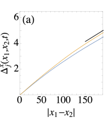
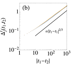
Figure 2: Spatial and temporal phase fluctuation functions $\Delta_{j}^{x}(x_{1},x_{2},t)$ and $\Delta_{j}^{t}(t_{1},t_{2})$ for the same set of parameters as the one in Fig. 1(c1) with system size $L=2^{10}$. (a) Scaling behavior of spatial phase fluctuation function $\Delta_{j}^{x}(x_{1},x_{2},t)$ on a linear scale. The black solid line corresponds to a linear function of $|x_{1}-x_{2}|$. The lower and upper curve correspond to $\Delta_{1}^{x}(x_{1},x_{2},t)$ and $\Delta_{2}^{x}(x_{1},x_{2},t)$, respectively, both of which show linear behavior at relatively large distances. (b) Scaling behavior of the temporal phase fluctuation function $\Delta_{j}^{t}(t_{1},t_{2})$ on a double logarithmic scale. The black solid line corresponds to a power law $\propto|t_{1}-t_{2}|^{2/3}$. The lower and upper curves correspond to $\Delta_{1}^{t}(t_{1},t_{2})$ and $\Delta_{2}^{t}(t_{1},t_{2})$, respectively, where one can observe the power law behavior at large time differences. Both the spatial and temporal phase fluctuation functions show scaling behavior that is consistent with the universality class of the 1D single-component KPZ equation. See text for more details.

5 Experimental observability

For the KPZ physics of the two-component DOC in its miscible phase, we expect the characteristic signatures are observable in the two-point spatial and temporal correlation functions $C_{j}^{x}(x_{1},x_{2},t)\equiv\langle\psi_{j}^{*}(x_{1},t)\psi_{j}(x_{2},t)\rangle$ and $C_{j}^{t}(t_{1},t_{2})\equiv L^{-1}\int_{x}\langle\psi_{j}^{*}(x,t_{1})\psi_{j}(x,t_{2})\rangle$ in the system’s steady state, i.e., $t,t_{1},t_{2}>T_{s}$, both of which are accessible in exciton-polariton experiments [1, 4, 3]. More specifically, from the long wavelength scaling behavior of the two-component DOC presented previously, we expect $C_{j}^{x}(x_{1},x_{2},t)\propto e^{-A_{j}|x_{1}-x_{2}|^{2\alpha}}$ and $C_{j}^{t}(t_{1},t_{2})\propto e^{-B_{j}|t_{1}-t_{2}|^{2\beta}}$, where $\alpha=1/2$, $\beta=1/3$ are the static and growth exponent for the 1D single-component KPZ equation [25, 38], respectively, and $A_{j},B_{j}$ are two nonuniversal positive constants determined by the microscopic details of the system. Fig. 3 shows the decay behavior of the spatial and temporal correlation function $C_{j}^{x}(x_{1},x_{2},t)$ and $C_{j}^{t}(t_{1},t_{2})$ for the same set of parameters as the one for Fig. 1(c1). Indeed, we observe that the decay behavior of both spatial and temporal correlation function are consistent with the expectations from the universality class of the KPZ equation.

       

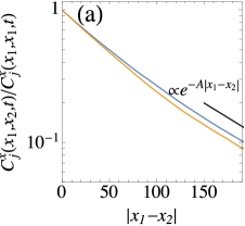
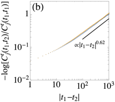
Figure 3: The decay behavior of the spatial and temporal correlation functions $C_{j}^{x}(x_{1},x_{2},t)$ and $C_{j}^{t}(t_{1},t_{2})$ for the same set of parameters as the one in Fig. 1(c1) with system size $L=2^{10}$. (a) Spatial correlation function $C_{j}^{x}(x_{1},x_{2},t)$ on a semi-logarithmic scale. The black solid line corresponds to a exponential function $\propto e^{-A|x_{1}-x_{2}|}$. The upper and lower curve correspond to $C_{1}^{x}(x_{1},x_{2},t)$ and $C_{2}^{x}(x_{1},x_{2},t)$, respectively, both of which show an exponential decay at relatively large distances. (b) The dependence of $-\log[C_{j}^{t}(t_{1},t_{2})/C_{j}^{t}(t_{1},t_{1})]$ on $|t_{1}-t_{2}|$ on a double-logarithmic scale. The black solid line corresponds to a power law function $\propto|t_{1}-t_{2}|^{0.62}$. The lower and upper curve correspond to $C_{1}^{t}(t_{1},t_{2})$ and $C_{2}^{t}(t_{1},t_{2})$, respectively, both of which show the sub-exponential decay behavior at relatively large time differences. A linear fit to the data points with $|t_{1}-t_{2}|\in[10^{2},10^{3}]$ gives rise to $\beta=0.31$. We observe that the decay behavior of both spatial and temporal correlation functions are consistent with the universality class of the 1D single-component KPZ equation.

Our discussion is based on a generic model for two-component DOC, hence we expect it is relevant for different experimental realizations. Currently, the most promising realization could come from the two-component polariton condensate systems, where the two different components correspond to the two different polarization directions of the photonic part of the polaritons [6, 7, 8, 9]. We can see from Fig. 1(a) that both the coherent and the dissipative inter-component interaction can drive the miscible-immiscible transition. In particular, the recently achieved tunability of inter-component coupling strengths via the polaritonic Feshbach resonance [6] gives rise to an intriguing platform for experimental investigations on the miscible-immiscible transition phenomenon in two-component DOCs established in this work. We expect that single experimental runs should indeed reveal the fragmentation of the driven open condensate in real space, leaving a clear fingerprint of the immiscible phase in one dimension. Moreover, the scaling of the temporal coherence function is expected to exhibit a difference from the one of the miscible phase, which manifests itself beyond the new scale set by the typical size of the phase separated domains.

Finally, we remark that compared to current typical setups in experiments for two-component polariton condensates  [6, 7, 8, 9], for instance, those investigating the polarization dynamics of polariton condensates [7, 8, 9], the model for two-component DOCs studied here possesses a higher symmetry, namely an invariance under independent phase rotations for different components, i.e., $\psi_{j}\rightarrow\psi_{j}e^{i\phi_{j}}$. The presence of this symmetry warrants the interesting physical scenarios discussed previously. In particular, it gives rise to a more interesting two-component KPZ equation for the miscible phase that possibly hosts nonequilibrium dynamical scaling behavior beyond the one of the single-component KPZ equation as shortly mentioned in Sec. 4.2. Although there exists rich physics even in the absence of the independent phase rotation symmetry, in both purely coherent [45] and driven-open [8] two-component condensates, in order to experimentally investigate the physics discussed in current work, one should reduce and ideally completely eliminate the strength of factors in experiments that can cause the breaking of independent phase rotation symmetry. For instance, asymmetry at the interfaces of quantum-wells, or the anisotropy-induced splitting of linear polarizations in the microcavity [8, 9] should be kept as small as possible, so that the physical effects originating from the weak breaking of the independent phase rotation symmetry are negligible at the typical spatio-temporal scale in experiments.

In fact for the KPZ physics, we do not expect observable modifications when independent phase rotation symmetry is absent. This is due to the fact that the effective description of the system in this case is expected to be directly described by the single-component KPZ equation that corresponds to the identical phase rotation symmetry for both components, i.e., $\psi_{j}\rightarrow\psi_{j}e^{i\phi}$. To check the robustness of the miscible-immiscible transition against symmetry breaking perturbations, we checked a concrete case where the system is exposed to a weak single-particle inter-component exchange process whose strength is around $5\%$ of $r_{j,c}$ in the case of Figs. 1(b1,b2). We found the misible-immiscible transition phenomenon is not substantially changed (see C for more details).

6 Conclusions and outlook

Two-component DOCs give rise to a novel scenario for the miscible-immiscible transition compared to its purely closed system counterpart, since the dynamical resources that cause the transition are qualitatively changed due to the absence of particle number and momentum conservation. In particular, the transition is driven predominantly by the gapped density fluctuations generated via the inter-component dissipative coupling. Below the transition in the miscible phase, we find the low frequency dynamics of the system to be effectively described by a two-component KPZ equation, which however belongs to the same nonequilibrium universality class as the single-component KPZ equation in 1D at generic choices of parameters. We believe that our work will stimulate further theoretical and experimental investigations on multicomponent DOCs. On the experimental side, the observation of the miscible-immiscible transition in a driven-open context in multicomponent polariton systems would complement the closed system counterpart observed in ultracold atoms [27, 28, 29] in a fundamentally different physical context, underpinning the generality of this phenomenon. On the theoretical side, the investigation of the high noise level and strong nonequilibrium regimes appears most interesting, where the phase compactness as an ingredient beyond the usual KPZ scenario must be expected to play a crucial role.

Appendix A Miscible-immiscible transition

In this appendix, we present some calculation details involved in the discussion for the miscible-immiscible transition.

It is easy to notice that $r_{j,c}$ can be chosen in such a way that there exists a stationary, spatially uniform solution for the two-component CGLE, i.e., the deterministic part of the two-component SCGLE in Eq. (1),

$$\partial_{t}\psi_{j} = \left(K_{j}\partial_{x}^{2}+r_{j}-u_{j}|\psi_{j}|^{2}-v|\psi_{\bar{j}}|^{2}\right)\psi_{j},$$ (19)

which reads $\psi_{j}^{(0)}(x,t)=M_{j}$ as shown in the main text. Here, $M_{j}$ is the solution for the real homogenous part of the two-component CGLE, i.e., $r_{j,d}-u_{j,d}M_{j}^{2}-v_{d}M_{\bar{j}}^{2}=0,$ whose explicit form reads $M_{j}^{2}=(r_{j,d}u_{\bar{j},d}-r_{\bar{j},d}v_{d})/(u_{1,d}u_{2,d}-v_{d}^{2})$. For a generic choice of parameters, the existence of the solution for $M_{1}^{2}$ and $M_{2}^{2}$ requires

$$\det\left(\begin{array}[]{cc}u_{1.d}&v_{d}\\ v_{d}&u_{2,d}\end{array}\right)=u_{1,d}u_{2,d}-v_{d}^{2}\neq 0.$$ (20)

We notice that there is an additional constraint on the parameters originating from $M_{j}^{2}>0$, which gives rise to

$$\frac{v_{d}}{u_{2,d}}>\frac{r_{1,d}}{r_{2,d}}>\frac{u_{1,d}}{v_{d}},\,\mathrm{if}\,u_{1,d}u_{2,d}-v_{d}^{2}>0,\,\mathrm{and}\,\frac{v_{d}}{u_{2,d}}<\frac{r_{1,d}}{r_{2,d}}<\frac{u_{1,d}}{v_{d}},\,\mathrm{if}\,u_{1,d}u_{2,d}-v_{d}^{2}<0.$$ (21)

The above stationary, spatially uniform solution is not always stable against small fluctuations. In the following, we perform a leading order stability analysis following a similar approach that has been applied to the coherent two-component BEC in Ref. [30]. As we have seen in the main text, the dispersion relation of eigenmodes $\omega_{a,k}$ up to the leading order in momentum can be expressed in a compact form by the help of three polynomials, $\mathcal{C}_{0},\mathcal{C}_{1},$ and $\mathcal{C}_{2}$ in terms of $M_{j},K_{j,\kappa}u_{j,\kappa},v_{\kappa}$, whose explicit forms read

$$\mathcal{C}_{0}=4M_{1}^{2}M_{2}^{2}\left[K_{1,c}\left(u_{1,c}K_{2,d}u_{2,d}-v_{c}v_{d}K_{2,d}+K_{2,c}u_{1,c}u_{2,c}-v_{c}^{2}K_{2,c}\right)\right.$$ (22)

$$\left.+K_{1,d}\left(K_{2,c}u_{2,c}u_{1,d}-v_{c}v_{d}K_{2,c}+K_{2,d}u_{1,d}u_{2,d}-v_{d}^{2}K_{2,d}\right)\right],$$

$$\mathcal{C}_{1}=4M_{1}^{2}M_{2}^{2}\left[K_{2,c}u_{2,c}u_{1,d}+K_{1,c}u_{1,c}u_{2,d}-v_{c}v_{d}\left(K_{1,c}+K_{2,c}\right)+K_{1,d}u_{1,d}u_{2,d}\right.$$ (23)

$$\left.+K_{2,d}u_{1,d}u_{2,d}-v_{d}^{2}\left(K_{1,d}+K_{2,d}\right)\right],$$

$$\mathcal{C}_{2}=2\left[M_{1}^{2}K_{1,c}u_{1,c}+M_{2}^{2}K_{2,c}u_{2,c}+M_{1}^{2}\left(K_{1,d}+2K_{2,d}\right)u_{1,d}+M_{2}^{2}\left(2K_{1,d}+K_{2,d}\right)u_{2,d}\right].$$

Requiring $\omega_{2,4}<0$ gives rise to the miscible condition $\mathcal{C}_{1}>0$ and simultaneously $\mathcal{C}_{0}>0$, whose explicit form reads

$$\tilde{v}_{c}<\frac{\sqrt{\mathcal{R}(u_{1})\mathcal{R}(u_{2})}}{\tilde{v}_{d}}\left[\mathcal{R}(K_{1}+K_{2})+\frac{1}{(K_{1,c}+K_{2,c})}\left(\frac{K_{2,c}}{\mathcal{R}(u_{2})}+\frac{K_{1,c}}{\mathcal{R}(u_{1})}\right)\right]$$

$$\mathrm{and\,simultaneously}$$

$$\tilde{v}_{c}<\left\{1+\mathcal{R}(K_{1})\mathcal{R}(u_{1})+\mathcal{R}(K_{2})\mathcal{R}(u_{2})+\mathcal{R}(K_{1})\mathcal{R}(u_{1})\mathcal{R}(K_{2})\mathcal{R}(u_{2})\cdot(1-\tilde{v}_{d}^{2})\right.$$ (25)

$$\left.+\left[\frac{1}{2}\sqrt{\mathcal{R}(u_{1})\mathcal{R}(u_{2})}\left(\mathcal{R}(K_{1})+\mathcal{R}(K_{2})\right)\tilde{v}_{d}\right]^{2}\right\}^{1/2}-\frac{1}{2}\sqrt{\mathcal{R}(u_{1})\mathcal{R}(u_{2})}\left(\mathcal{R}(K_{1})+\mathcal{R}(K_{2})\right)\tilde{v}_{d},$$

where $\tilde{v}_{c}\equiv v_{c}/\sqrt{u_{1,c}u_{2,c}}$ and $\tilde{v}_{d}\equiv v_{d}/\sqrt{u_{1,d}u_{2,d}}$ are the rescaled dimensionless inter-component coherent and dissipative coupling strength, respectively, and the definition $\mathcal{R}(z)\equiv\Re(z)/\Im(z)$ for $z\in\mathbb{C}$. Notice that the two conditions $\mathcal{C}_{1}>0$ and $\mathcal{C}_{0}>0$ are independent, therefore one should generically solve these two inequalities and take the overlap region indicated by the two.

When $r_{1,d}=r_{2,d}\equiv r_{d},u_{1,d}=u_{2,d}\equiv u_{d},v_{d}=0$, $\omega_{1}^{(0)}$ and $\omega_{3}^{(0)}$ are degenerate, and the dispersion relation assumes the following form

$$\omega_{a,k}=-2M^{2}u_{d}-\frac{k^{2}}{2u_{d}}\left\{\pm\left(-K_{1,c}u_{1,c}-K_{2,c}u_{2,c}+u_{d}K_{1,d}+u_{d}K_{2,d}\right)\right.$$ (26)

$$+\left[-2K_{1,c}\left(u_{d}u_{1,c}K_{1,d}-u_{d}u_{1,c}K_{2,d}+K_{2,c}u_{1,c}u_{2,c}-2v_{c}^{2}K_{2,c}\right)\right.$$

$$\left.\left.+\left(K_{2,c}u_{2,c}+u_{d}K_{1,d}-u_{d}K_{2,d}\right){}^{2}+K_{1,c}^{2}u_{1,c}^{2}\right]^{1/2}\right\},\,\mathrm{for}\,a=1,3,$$

$$\omega_{a,k}=-\frac{k^{2}}{2u_{d}}\left\{\left(K_{1,c}u_{1,c}+K_{2,c}u_{2,c}+u_{d}K_{1,d}+u_{d}K_{2,d}\right)\right.$$ (27)

$$\pm\left[-2K_{1,c}\left(-u_{d}u_{1,c}K_{1,d}+u_{d}u_{1,c}K_{2,d}+K_{2,c}u_{1,c}u_{2,c}-2v_{c}^{2}K_{2,c}\right)\right.$$

$$\left.\left.+\left(K_{2,c}u_{2,c}-u_{d}K_{1,d}+u_{d}K_{2,d}\right){}^{2}+K_{1,c}^{2}u_{1,c}^{2}\right]^{1/2}\right\},\,\mathrm{for}\,a=2,4,$$

where $M\equiv r_{d}/u_{d}$.

Appendix B Derivation of the two-component KPZ equation as the effective description for two-component DOCs

In this appendix, we present the derivation details for the low frequency effective description of two-component DOCs, which can be straightforwardly applied to the generic multi-component case.

From the equation of motion (EOM) for DOCs, we can directly write down the EOM for the real and imaginary part of $\psi_{j}$, denoted as $\psi_{j,a}$, with $a=1,2$, i.e., $\psi_{j}=\psi_{j,1}+i\psi_{j,2}$. The generic form of the dynamical equation for $\psi_{j,a}$ reads

$$\partial_{t}\psi_{j,a}=F_{j,a}[\{\psi_{j,a}\}].$$ (28)

In order to derive a set of dynamical equations for $\rho_{j},\theta_{j}$, where $\psi_{j,1}=\rho_{j}\cos\theta_{j}$, $\psi_{j,2}=\rho_{j}\sin\theta_{j}$, we can make use of the Jacobian matrix between $\{\psi_{j,a}\}$ and $\{\rho_{j},\theta_{j}\}$, i.e.,

$$\left(\begin{array}[]{c}\partial_{t}\rho_{1}\\ \partial_{t}\theta_{1}\\ \partial_{t}\rho_{2}\\ \partial_{t}\theta_{2}\end{array}\right) = \left(\begin{array}[]{cccc}\cos\theta_{1}&-\rho_{1}\sin\theta_{1}&0&0\\ \sin\theta_{1}&\rho_{1}\cos\theta_{1}&0&0\\ 0&0&\cos\theta_{2}&-\rho_{2}\sin\theta_{2}\\ 0&0&\sin\theta_{2}&\rho_{2}\cos\theta_{2}\end{array}\right)^{-1}\left(\begin{array}[]{c}\partial_{t}\psi_{1,1}\\ \partial_{t}\psi_{1,2}\\ \partial_{t}\psi_{2,1}\\ \partial_{t}\psi_{2,2}\end{array}\right).$$ (41)

After plugging the EOM for $\psi_{j,a}$ Eq. (28) into the above equation, and substituting $\psi_{i,1}=\rho_{i}\cos\theta_{i}$, $\psi_{i,2}=\rho_{i}\sin\theta_{i}$, we arrive at the EOM for the amplitude and the phase fields, i.e.,

$$\left(\begin{array}[]{c}\partial_{t}\rho_{1}\\ \partial_{t}\theta_{1}\\ \partial_{t}\rho_{2}\\ \partial_{t}\theta_{2}\end{array}\right)=\left(\begin{array}[]{cccc}\cos\theta_{1}&\sin\theta_{1}&0&0\\ -\rho_{1}^{-1}\sin\theta_{1}&\rho_{1}^{-1}\cos\theta_{1}&0&0\\ 0&0&\cos\theta_{2}&\sin\theta_{2}\\ 0&0&-\rho_{2}^{-1}\sin\theta_{2}&\rho_{2}^{-1}\cos\theta_{2}\end{array}\right)\left(\begin{array}[]{c}F_{1,1}[\{\rho_{j},\theta_{j}\}]\\ F_{1,2}[\{\rho_{j},\theta_{j}\}]\\ F_{2,1}[\{\rho_{j},\theta_{j}\}]\\ F_{2,2}[\{\rho_{j},\theta_{j}\}]\end{array}\right).$$ (54)

(55)

The following steps in the derivation go along the lines of the similar discussion presented in Ref. [17] as we outline below. We first decompose the amplitude field $\rho_{j}(x,t)$ into the sum of the stationary, spatially uniform amplitude $|\psi_{j}^{(0)}(x,t)|=M_{j}$ and the amplitude fluctuation $\chi_{j}(x,t)$ on its top, i.e., $\rho_{j}(x,t)=M_{j}+\chi_{j}(x,t)$. After substituting this decomposition into Eq. (55), we arrive at a EOM for amplitude and phase fluctuations. Since the dynamics of the gapped amplitude fluctuation $\chi_{j}(x,t)$ is fast compared to the gapless phase fluctuations, we can further adiabatically eliminate $\chi_{j}(x,t)$ and arrive at the two-component KPZ equation Eq. (18) for the phase fields $\theta_{i}(x,t)$, upon keeping only the terms that are not irrelevant in the RG sense. The explicit forms for the parameters in the two-component KPZ equation Eq. (18) read

$$D_{11} = \mathcal{A}\left(K_{1,c}u_{1,c}u_{2,d}+K_{1,d}u_{1,d}u_{2d}-K_{1,c}v_{c}v_{d}-K_{1,d}v_{d}^{2}\right),$$ (56)

$$D_{22} = \mathcal{A}\left(K_{2,c}u_{2,c}u_{1,d}+K_{2,d}u_{2,d}u_{1,d}-K_{2,c}v_{c}v_{d}-K_{2,d}v_{d}^{2}\right),$$ (57)

$$D_{12} = \mathcal{A}K_{2,c}\left(u_{1,d}v_{c}-u_{1,c}v_{d}\right),$$ (58)

$$D_{21} = \mathcal{A}K_{1,c}\left(u_{2,d}v_{c}-u_{2,c}v_{d}\right),$$ (59)

$$\lambda_{11} = \left(K_{1,d}u_{1,c}u_{2,d}-K_{1,c}u_{1,d}u_{2d}-K_{1,d}v_{c}v_{d}+K_{1,c}v_{d}^{2}\right),$$ (60)

$$\lambda_{22} = \left(K_{2,d}u_{2,c}u_{1,d}-K_{2,c}u_{2,d}u_{1d}-K_{2,d}v_{c}v_{d}+K_{2,c}v_{d}^{2}\right),$$ (61)

$$\lambda_{12} = K_{2,d}\left(u_{1,d}v_{c}-u_{1,c}v_{d}\right),$$ (62)

$$\lambda_{21} = K_{1,d}\left(u_{2,d}v_{c}-u_{2,c}v_{d}\right),$$ (63)

$$\sigma_{1}^{\mathrm{KPZ}} = \frac{1}{M_{1}^{2}}\left(1+\mathcal{\mathcal{A}}^{2}\left(u_{1,c}u_{2,d}-v_{c}v_{d}\right)^{2}\right)\sigma_{1}+\frac{1}{M_{2}^{2}}\mathcal{A}^{2}\left(u_{1,d}v_{c}-u_{1,c}v_{d}\right)^{2}\sigma_{2},$$ (64)

$$\sigma_{2}^{\mathrm{KPZ}} = \frac{1}{M_{2}^{2}}\left(1+\mathcal{A}^{2}\left(u_{2,c}u_{1,d}-v_{c}v_{d}\right)^{2}\right)\sigma_{2}+\frac{1}{M_{1}^{2}}\mathcal{A}^{2}\left(u_{2,d}v_{c}-u_{2,c}v_{d}\right)^{2}\sigma_{1},$$ (65)

with $\mathcal{A}\equiv\left(u_{1,d}u_{2,d}-v_{d}^{2}\right)^{-1}$.

Appendix C Effects of weak breaking of independent phase rotation symmetry

As mentioned in the main text, in current experimental setups for two-component polariton condensates [7, 6, 8, 9], there exist physical processes that can break the independent phase rotation symmetry. One type of these processes is the single particle inter-component exchange [8, 9] that corresponds to a term $\varepsilon\psi_{\bar{j}}$ appearing in the right hand side of the dynamical equation for $\psi_{j}$ Eq. (1), i.e., the EOM of the system in the presence the single particle inter-component exchange reads

$$\partial_{t}\psi_{j}=\left(K_{j}\partial_{x}^{2}+r_{j}-u_{j}|\psi_{j}|^{2}-v|\psi_{\bar{j}}|^{2}\right)\psi_{j}+\varepsilon\psi_{\bar{j}}+\zeta_{j}.$$ (66)

Here $\varepsilon$ is a complex number, i.e., $\varepsilon=\varepsilon_{d}+i\varepsilon_{c}$, whose real and imaginary part characterize the dissipative and coherent inter-component exchange rate, respectively. Its magnitude $|\varepsilon|$ directly gives rise to a time scale $T_{B}\propto|\varepsilon|^{-1}$ and a length scale $L_{B}\propto|\varepsilon|^{-1/z}$(with $z$ being the dynamical exponent of the system), beyond which the physical effects associated to the breaking of the symmetry are expected to manifest themselves. This indicates that as long as $|\varepsilon|$ is small enough such that the associated spatial (temporal) scale $L_{B}$ ($T_{B}$) is larger than the spatial (temporal) scale beyond which the physical phenomena predicted by the theory with the independent phase rotation symmetry could appear, the corresponding physical phenomena are expected not to be substantially affected.

As a concrete example, in Fig. 4, we show two snapshots of the density distribution at different time of a system in the presence of weak inter-component exchange processes. Except $|\varepsilon|$ being around $5\%$ of $r_{j,c}$, all other parameters corresponding to Fig. 4 are exactly the same as those in Figs. 1(b1,b2), i.e., the system is expected to evolve into an immiscible phase despite being initialized with a generic homogeneous configuration in the miscible phase. As we can see from Fig. 4, in the presence of small $|\varepsilon|$, the system still show a similar evolution as the case with $|\varepsilon|=0$ [cf. Figs. 1(b1,b2)], indicating that the effects of weak symmetry breaking term are not substantial in this case.

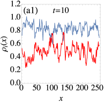
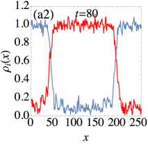
Figure 4: Snapshots of distributions of condensate field amplitudes $\rho_{j}(x)\equiv|\psi_{j}(x)|$ at different time (the blue and red curve correspond to $\rho_{1}(x)$ and $\rho_{2}(x)$, respectively) of a system in the presence of a weak inter-component exchange term with $\varepsilon_{d}=\varepsilon_{c}=0.003$, where an immiscible phase is clearly observed at a later time ($t=80$). The values of all other parameters are the same as those in Figs. 1(b1,b2). See text for more details.

References

- [1] J. Kasprzak, M. Richard, S. Kundermann, A. Baas, P. Jeambrun, J. M. J. Keeling, F. M. Marchetti, M. H. Szymańska, R. Andre, J. L. Staehli, V. Savona, P. B. Littlewood, B. Deveaud, and L. S. Dang, Nature (London) 443, 409 (2006);
- [2] K. G. Lagoudakis, M. Wouters, M. Richard, A. Baas, I. Carusotto, R. Andre, Le Si Dang, and B. Deveaud-Pledran, Nat. Phys. 4, 706 (2008);
- [3] A. P. D. Love, D. N. Krizhanovskii, D. M. Whittaker, R. Bouchekioua, D. Sanvitto, S. A. Rizeiqi, R. Bradley, M. S. Skolnick, P. R. Eastham, R. André, and L. S. Dang, Phys. Rev. Lett. 101, 067404 (2008).
- [4] G. Roumpos, M. Lohse, W. H. Nitsche, J. Keeling, M. H. Szymańska, P. B. Littlewood, A. Löffler, S. Höfling, L. Worschech, A. Forchel, and Y. Yamamoto, PNAS 109, 6467 (2012).
- [5] E. Wertz, A. Amo, D. D. Solnyshkov, L. Ferrier, T. C. H. Liew, D. Sanvitto, P. Senellart, I. Sagnes, A. Lemaître, A. V. Kavokin, G. Malpuech, and J. Bloch, Phys. Rev. Lett. 109, 216404 (2012).
- [6] N. Takemura, S. Trebaol, M. Wouters, M. T. Portella-Oberli, and B. Deveaud, Nat. Phys. 10, 500 (2014).
- [7] J. Fischer, S. Brodbeck, A. V. Chernenko, I. Lederer, A. Rahimi-Iman, M. Amthor, V. D. Kulakovskii, L. Worschech, M. Kamp, M. Durnev, C. Schneider, A. V. Kavokin, and S. Höfling, Phys. Rev. Lett. 112, 093902 (2014).
- [8] H. Ohadi, A. Dreismann, Y. G. Rubo, F. Pinsker, Y. del Valle-Inclan Redondo, S. I. Tsintzos, Z. Hatzopoulos, P. G. Savvidis, and J. J. Baumberg, Phys. Rev. X 5, 031002 (2015).
- [9] A. Askitopoulos, K. Kalinin, T. C. H. Liew, P. Cilibrizzi, Z. Hatzopoulos, P. G. Savvidis, N. G. Berloff, and P. G. Lagoudakis, Phys. Rev. B 93, 205307 (2016).
- [10] N. Syassen, D. M. Bauer, M. Lettner, T. Volz, D. Dietze, J. J. García-Ripoll, J. I. Cirac, G. Rempe, and S. Dürr, Science 320, 1329 (2008).
- [11] C. Carr, R. Ritter, C. G. Wade, C. S. Adams, and K. J. Weatherill, Phys. Rev. Lett. 111, 113901 (2013).
- [12] B. Zhu, B. Gadway, M. Foss-Feig, J. Schachenmayer, M. L. Wall, K. R. A. Hazzard, B. Yan, S. A. Moses, J. P. Covey, D. S. Jin, J. Ye, M. Holland, and A. M. Rey, Phys. Rev. Lett. 112, 070404 (2014).
- [13] R. Blatt and C. Roos, Nat. Phys. 8, 277 (2012).
- [14] J. W. Britton, B. C. Sawye[31, 32, 17, 33, 8, 9]r, A. C. Keith, C.-C. J. Wang, J. K. Freericks, H. Uys, M. J. Biercuk, and J. J. Bollinger, Nature (London) 484, 489 (2012).
- [15] M. Hartmann, F. Brandao, and M. Plenio, Laser Photonics Rev. 2, 527 (2008).
- [16] A. A. Houck, H. E. Tureci, and J. Koch, Nat. Phys. 8, 292 (2012).
- [17] E. Altman, L. M. Sieberer, L. Chen, S. Diehl, and J. Toner, Phys. Rev. X 5, 011017 (2015).
- [18] V. N. Gladilin, K. Ji, and M. Wouters, Phys. Rev. A 90, 023615 (2014).
- [19] K. Ji, V. N. Gladilin, and M. Wouters, Phys. Rev. B 91, 045301 (2015).
- [20] L. He, L. M. Sieberer, E. Altman, and S. Diehl, Phys. Rev. B 92, 155307 (2015).
- [21] S. Mathey, T. Gasenzer, and J. M. Pawlowski, Phys. Rev. A 92, 023635 (2015).
- [22] G. Wachtel, L. M. Sieberer, S. Diehl, and E. Altman, Phys. Rev. B 94, 104520 (2016).
- [23] L. M. Sieberer, G. Wachtel, E. Altman, and S. Diehl, Phys. Rev. B 94, 104521 (2016).
- [24] L. He, L. M. Sieberer, and S. Diehl, Phys. Rev. Lett. 118, 085301 (2017).
- [25] M. Kardar, G. Parisi, and Y. C. Zhang, Phys. Rev. Lett. 56, 889 (1986).
- [26] D. M. Stamper-Kurn and M. Ueda, Rev. Mod. Phys. 85, 1191 (2013).
- [27] C. J. Myatt, E. A. Burt, R. W. Ghrist, E. A. Cornell, and C. E. Wieman, Phys. Rev. Lett. 78, 586 (1997).
- [28] D. S. Hall, M. R. Matthews, J. R. Ensher, C. E. Wieman, and E. A. Cornell, Phys. Rev. Lett. 81, 1539 (1998).
- [29] E. Nicklas, H. Strobel, T. Zibold, C. Gross, B. A. Malomed, P. G. Kevrekidis, and M. K. Oberthaler, Phys. Rev. Lett. 107, 193001 (2011).
- [30] E. Timmermans, Phys. Rev. Lett. 81, 5718 (1998).
- [31] M. Wouters and I. Carusotto, Phys. Rev. Lett. 99, 140402 (2007).
- [32] I. Carusotto and C. Ciuti, Rev. Mod. Phys. 85, 299 (2013).
- [33] F. Pinsker and H. Flayac, Phys. Rev. Lett. 112, 140405 (2014).
- [34] X. Xu, Y. Hu, Z. Zhang, and Z. Liang, arXiv:1704.08439.
- [35] K. Kasamatsu and M. Tsubota, Phys. Rev. Lett. 93, 100402 (2004).
- [36] L. He and S. Yi, Phys. Rev. A 80, 033618 (2009).
- [37] I. Vidanović, N. J. van Druten, and M. Haque, New Journal of Physics, 15, 035008 (2013).
- [38] T. Halpin-Healy and Y. C. Zhang, Phys. Rep. 254, 215 (1995).
- [39] D. Ertaş, and M. Kardar, Phys. Rev. Lett. 69, 929 (1992).
- [40] P. L. Ferrari, T. Sasamoto, and H. Spohn, J. Stat. Phys. 153, 377 (2013).
- [41] V. Popkov, J. Schmidt, and G. M. Schütz, Phys. Rev. Lett 112, 200602 (2014).
- [42] H. Spohn, G. Stoltz, J. Stat. Phys. 160, 861 (2015).
- [43] V. Popkov, J. Schmidt, and G. M. Schütz, J. Stat. Phys. 160, 835 (2015).
- [44] V. Popkov, A. Schadschneider, J.Schmidt, and G. M. Schütz, PNAS 112, 12645 (2015).
- [45] E. Nicklas, M. Karl, M. Höfer, A. Johnson, W. Muessel, H. Strobel, J. Tomkovič, T. Gasenzer, and M. K. Oberthaler, Phys. Rev. Lett. 115, 245301 (2015).