An Integrated Quadratic Reconstruction for Finite Volume Schemes to Scalar Conservation Laws in Multiple Dimensions

Abstract

We proposed a piecewise quadratic reconstruction method in multiple dimensions, which is in an integrated style, for finite volume schemes to scalar conservation laws. This integrated quadratic reconstruction is parameter-free and applicable on flexible grids. We show that the finite volume schemes with the new reconstruction satisfy a local maximum principle with properly setup on time steplength. Numerical examples are presented to show that the proposed scheme attains a third-order accuracy for smooth solutions in both 2D and 3D cases. It is indicated by numerical results that the local maximum principle is helpful to prevent overshoots in numerical solutions.

1 Introduction

The study of robust, accurate, and efficient finite volume schemes for conservation laws is an active research area in computational fluid dynamics. It was noted that higher-order finite volume methods have been shown to be more efficient than second-order methods [1]. The key element in the reconstruction procedures of high-order schemes is suppressing non-physical oscillations near discontinuities, while achieving high-order accuracy in smooth regions. One of the pioneering work in this area is the finite volume scheme based on the $k$-exact reconstruction, first proposed by Barth and Fredrichson [2] and later extended to the cell-centered finite volume scheme by Mitchell and Walters [3]. For more recent work on the use of $k$-exact reconstruction to attain high-order accuracy, we refer the reader to [4, 5, 1, 6, 7] for instance. The hierarchical reconstruction strategies of Liu et al. [8] were also used to achieve higher-order accuracy [9, 10], where the information is recomputed level by level from the highest order terms to the lowest order terms with certain non-oscillatory method. Other type of high-order finite volume schemes includes the WENO scheme [11]. Although the implementation of WENO scheme is comparatively complicated on unstructured meshes due to the needs of identifying several candidate stencils and performing a reconstruction on each stencil [6], it has been successfully applied on the unstructured meshes for both two-dimensional triangulations [12, 13, 14, 15, 16, 17] and three-dimensional triangulations [18, 19]. Most of these schemes do not lead to a strict maximum principle, while they are essentially non-oscillatory [20]. Actually, the reconstruction procedure for maximum-principle-satisfying second-order schemes are relatively mature [21, 22, 23, 24, 25, 26], while there are few maximum-principle-satisfying reconstruction approaches for higher-order finite volume schemes on unstructured meshes.

Limiting to scalar conservation laws, a quadratic reconstruction for finite volume schemes applicable on 2D and 3D unstructured meshes is developed in this paper. The construction is a further exploration of the integrated linear reconstruction (ILR) in [27, 28], where the coefficients of reconstructed polynomial are embedded in an optimization problem. It is appealing for us to generalize the optimization-based constructions therein to an integrated quadratic reconstruction (IQR) such that the scheme achieves a third-order accuracy while satisfying a local maximum principle. It was pointed out in [29] that the scheme satisfying the standard local maximum principle is at most second-order accurate around extrema. To achieve higher than second-order accuracy, high-order information of the exact solution has to be taken into account in the definition of local maximum principle [29, 30]. Sanders [31] suggested to measure the total variation of approximation polynomials. Liu et al. [32] constructed a third-order non-oscillatory scheme by controlling the number of extrema and the range of the reconstructed polynomials. Zhang et al. constructed a genuinely high-order maximum-principle-satisfying finite volume schemes for multi-dimensional nonlinear scalar conservation laws on both rectangular meshes [33] and triangular meshes [34] by limiting the reconstructed polynomials around cell averages. The flux limiting technique developed by Christlieb et al. [35] is another family of maximum-principle-satisfying methods on unstructured meshes. In our scheme, it is proposed that the extrema of numerical solutions are measured by extrema of polynomial on a cluster of points, following the technique of Zhang et al. [33, 34]. To overcome the difficulty of loss of high-order information in cell averages, besides the cell averages at current time level, we utilize the reconstruction polynomials at previous time step. This idea is based on the wave propagation nature of conservation laws. Since the solution value at $({\bf x},t)$ can be tracked back to a point in the ball around ${\bf x}$ with radius as $v\Delta t$ at time $t-\Delta t$, while $v$ is local wave speed, it is reasonable for us to use the value in this ball at previous time step in the reconstruction. It is shown that this may lead to a third-order numerical scheme, meanwhile a local maximum principle is satisfied. An advantage of the new reconstruction is that there is no artificial parameter at all, which makes the algorithm robust and independent of the problem.

The rest of the paper is organized as follows. In Section 2, we describe the integrated quadratic reconstruction based on solving a series of quadratic programming problems. Section 3 is devoted to the discussion of the order of accuracy and maximum principle for scalar conservation laws. Numerical results are given to demonstrate the stability and accuracy of the proposed scheme in Section 4. Finally, a short conclusion is drawn in Section 5.

2 Numerical Scheme

Let us consider a scalar hyperbolic conservation law on a $d$-dimensional domain $\Omega$, $d=2,3$, as

$$\dfrac{\partial u}{\partial t}+\nabla\cdot\bm{F}(u)=0,$$ (1)

together with appropriate boundary condition and initial value $u(\cdot,0)$. The computational domain $\Omega$ is triangulated into a grid, either structured or unstructured, denoted by $\mathcal{T}$. For an arbitrary cell $T_{0}\in\mathcal{T}$ referred as a control volume for finite volume method, let $e_{j}$ be the facet of $T_{0}$ shared by $T_{0}$ and its von Neumann neighbor $T_{j}$, and $\bm{n}_{j}$ be the unit outer normal of $e_{j}$ $(j=1,\cdots,J)$. The finite volume discretization for (1) is then formulated as

$$\dfrac{u_{0}^{n+1}-u_{0}^{n}}{\Delta t_{n}}+\dfrac{1}{|T_{0}|}\sum_{j=1}^{J}\sum_{q=1}^{Q_{j}}w_{jq}\mathcal{F}(v_{h,0}^{n}(\bm{z}_{jq}),v_{h,j}^{n}(\bm{z}_{jq});\bm{n}_{j})|e_{j}|=0.$$ (2)

Here $u_{0}^{n}$ approximates the cell average of the solution $u$ on $T_{0}$ at $n$-th time level $t_{n}$, i.e.

$$u_{0}^{n}\approx\left.\Pi u(\cdot,t_{n})\right|_{T_{0}},$$

where $\Pi$ is the piecewise constant projection defined by

$$\left.\Pi w\right|_{T_{0}}=\mathchoice{{\vbox{\hbox{$\textstyle-$ }}\kern-7.83337pt}}{{\vbox{\hbox{$\scriptstyle-$ }}\kern-5.90005pt}}{{\vbox{\hbox{$\scriptscriptstyle-$ }}\kern-4.75003pt}}{{\vbox{\hbox{$\scriptscriptstyle-$ }}\kern-4.25003pt}}\!\int_{T_{0}}w(\bm{x})\mathrm{d}\bm{x}:=\dfrac{1}{|T_{0}|}\int_{T_{0}}w(\bm{x})\mathrm{d}\bm{x},\quad\forall w\in L^{1}(\Omega).$$

The point $\bm{z}_{jq}$ is the $q$-th quadrature point on the facet $e_{j}$ with weight $w_{jq}$ ($q=1,\cdots,Q_{j},j=1,\cdots,J$), the function $v_{h,0}^{n}(\bm{x})$ is a reconstructed polynomial computed from the patch of cell $T_{0}$, the function $v_{h,j}^{n}(\bm{x})$ ($j=1,\cdots,J$) is a reconstructed polynomial computed from the patch of cell $T_{j}$, and $\mathcal{F}(u,v;\bm{n})$ is a numerical flux, such as the Lax-Friedrichs flux

$$\mathcal{F}(u,v;\bm{n})=\dfrac{1}{2}(\bm{F}(u)+\bm{F}(v))\cdot\bm{n}-\dfrac{1}{2}a(v-u),$$ (3)

where $a=\sup\limits_{u,\bm{n}}|\bm{F}^{\prime}(u)\cdot\bm{n}|$ represents the maximal characteristic speed.

Denote the piecewise constant approximation of $u(\bm{x},t_{n})$ to be $u_{h}^{n}(\bm{x})$, which takes $u_{0}^{n}$ as its value on $T_{0}$. In this paper we will focus on constructing a quadratic polynomial $v_{h,0}^{n}(\bm{x})$ on each control volume $T_{0}$. And the resulting piecewise quadratic function on the whole domain $\Omega$ is denoted by $v_{h}^{n}(\bm{x})$. Classical patch reconstruction algorithms in the literature directly give $v_{h}^{n}(\bm{x})$ from $u_{h}^{n}(\bm{x})$, while the integrated quadratic reconstruction requires additional information. Precisely, we may formulate our reconstruction as an operator $\mathcal{R}_{h}$

$$v_{h}^{n}(\bm{x})=\mathcal{R}_{h}[u_{h}^{n},v_{h}^{n-1}](\bm{x}).$$

That is to say, the function $v_{h}^{n}$ depends on not only its piecewise constant counterpart $u_{h}^{n}$, but also the previous reconstruction $v_{h}^{n-1}$. Basically, the operator $\mathcal{R}_{h}$ accepts two functions as its arguments: the first function is a piecewise constant function on $\mathcal{T}$, and the second function is a piecewise continuous function on $\mathcal{T}$. With the introduction of the operator $\mathcal{R}_{h}$, the numerical scheme (2) can be formally identified as

$$u_{h}^{n+1}=u_{h}^{n}+\Delta t_{n}\mathcal{L}(v_{h}^{n}),\quad v_{h}^{n}=\mathcal{R}_{h}[u_{h}^{n},v_{h}^{n-1}],$$ (4)

where $\mathcal{L}$ is the operator defined through (2).

For the initial level $n=0$, we directly take $u_{h}^{0}(\bm{x})$ to be the piecewise constant projection of $u(\bm{x},0)$ on $\mathcal{T}$ and $v_{h}^{-1}(\bm{x})=u(\bm{x},0)$, saying

$$v_{h}^{0}(\bm{x})=\mathcal{R}_{h}[\Pi u(\cdot,0),u(\cdot,0)](\bm{x}),$$ (5)

to bootstrap the computation. And we note that (5) actually defines a mapping from a continuous function $w\in C(\Omega)\bigcap L^{1}(\Omega)$ to a piecewise quadratic function on $\mathcal{T}$. We denote this mapping again by $\mathcal{R}_{h}$

$$\mathcal{R}_{h}[w](\bm{x}):=\mathcal{R}_{h}[\Pi w,w](\bm{x}),$$

for convenience. Therefore, we need only to specify $\mathcal{R}_{h}$ to close the scheme (2). Below we describe the procedure to specify $v_{h}^{n}(\bm{x})$ on a single cell $T_{0}$ using $u_{h}^{n}(\bm{x})$ and $v_{h}^{n-1}(\bm{x})$.

The reconstructed quadratic function on cell $T_{0}$ can be formulated as

$$v_{h,0}^{n}(\bm{x})=u_{0}^{n}+\bm{L}\cdot(\bm{x}-\bm{x}_{0})+\dfrac{1}{2}\mathbf{H}:((\bm{x}-\bm{x}_{0})\otimes(\bm{x}-\bm{x}_{0})-\mathbf{J}_{0}),$$ (6)

where the operator $\otimes$ denotes the tensor product of vectors, and the operator $:$ denotes the inner-product of high order tensor. The vector $\bm{L}$ and the matrix $\mathbf{H}$ are

$$\bm{L}=\begin{bmatrix}L_{1}\\ L_{2}\\ \cdots\\ L_{d}\end{bmatrix}\quad\text{~{}and~{}}\quad\mathbf{H}=\begin{bmatrix}H_{11}&H_{12}&\cdots&H_{1d}\\ H_{21}&H_{22}&\cdots&H_{2d}\\ \vdots&\vdots&\ddots&\vdots\\ H_{d1}&H_{d2}&\cdots&H_{dd}\end{bmatrix},$$

approximates respectively the gradient $\nabla u$ and the Hessian $\nabla^{2}u$ near the centroid $\bm{x}_{0}$ of cell $T_{0}$, and $\mathbf{J}_{0}$ represents the second moments of the cell $T_{0}$

$$\mathbf{J}_{0}=\mathchoice{{\vbox{\hbox{$\textstyle-$ }}\kern-7.83337pt}}{{\vbox{\hbox{$\scriptstyle-$ }}\kern-5.90005pt}}{{\vbox{\hbox{$\scriptscriptstyle-$ }}\kern-4.75003pt}}{{\vbox{\hbox{$\scriptscriptstyle-$ }}\kern-4.25003pt}}\!\int_{T_{0}}(\bm{x}-\bm{x}_{0})\otimes(\bm{x}-\bm{x}_{0})\mathrm{d}\bm{x},$$

which depends on the geometry of control volume $T_{0}$ only. In Table 1 we list the second moments of several geometric shapes widely used in the mesh triangulation. Note that the quadratic polynomial (6) automatically satisfies the conservation property, i.e.

$$\mathchoice{{\vbox{\hbox{$\textstyle-$ }}\kern-7.83337pt}}{{\vbox{\hbox{$\scriptstyle-$ }}\kern-5.90005pt}}{{\vbox{\hbox{$\scriptscriptstyle-$ }}\kern-4.75003pt}}{{\vbox{\hbox{$\scriptscriptstyle-$ }}\kern-4.25003pt}}\!\int_{T_{0}}v_{h,0}^{n}(\bm{x})\mathrm{d}\bm{x}=u_{0}^{n}.$$

Table 1: Geometry parameters of several control volumes.

	Geometry a	Second moments b	$\nu$
Rectangle		$\displaystyle\mathbf{J}=\dfrac{1}{12}\begin{bmatrix}{l_{x}^{2}}&0\\ 0&{l_{y}^{2}}\end{bmatrix}$	$\dfrac{1}{16}$
Triangle		$\displaystyle\mathbf{J}=\dfrac{1}{36}\sum_{1\leq i<j\leq 3}\overrightarrow{P_{i}P_{j}}\otimes\overrightarrow{P_{i}P_{j}}$	$\dfrac{1}{12}$
Cuboid		$\displaystyle\mathbf{J}=\dfrac{1}{12}\begin{bmatrix}{l_{x}^{2}}&0&0\\ 0&{l_{y}^{2}}&0\\ 0&0&{l_{z}^{2}}\end{bmatrix}$	$\dfrac{1}{30}$
Tetrahedron		$\displaystyle\mathbf{J}=\dfrac{1}{80}\sum_{1\leq i<j\leq 4}\overrightarrow{P_{i}P_{j}}\otimes\overrightarrow{P_{i}P_{j}}$	$\dfrac{1}{20}$

• For segmental or rectangular facets, the quadrature points are the Gaussian points, while for triangular facets, the barycentric coordinates of three quadrature points are $(2/3,1/6,1/6)$, $(1/6,2/3,1/6)$ and $(1/6,1/6,2/3)$ respectively.

• $l$’s denote the dimensions of the control volume, and $P_{i}$’s denote the vertices of the control volume.

To suppress numerical oscillations we follow the same basic outline as traditional second-order limiters, namely, limiting the values on the quadrature points $\{\bm{z}_{jq}\}$. Note that higher-order reconstructions admit local extrema within cells, in contrast to linear reconstructions. Therefore, to improve the restriction within cells, we also examine the value at the centroid $\bm{x}_{0}$. For convenience, we define a cluster of collocation points associated to a given cell $T_{0}$ by

$$Z_{0}=\{\bm{z}_{jq}|q=1,\cdots,Q_{j},j=1,\cdots,J\}\cup\{\bm{x}_{0}\},$$

which consists of all quadrature points on the cell faces along with the centroid of the whole cell (see the geometry column in Table 1). Now introduce an objective function depending on the parameters $\bm{L}$ and $\mathbf{H}$ in the expression (6) of $v_{h,0}^{n}(\bm{x})$ as

$$\delta(\bm{L},\mathbf{H})=\sum_{i\in S}(\overline{u}_{i}^{n}-u_{i}^{n})^{2},\quad\overline{u}_{i}^{n}=\mathchoice{{\vbox{\hbox{$\textstyle-$ }}\kern-7.83337pt}}{{\vbox{\hbox{$\scriptstyle-$ }}\kern-5.90005pt}}{{\vbox{\hbox{$\scriptscriptstyle-$ }}\kern-4.75003pt}}{{\vbox{\hbox{$\scriptscriptstyle-$ }}\kern-4.25003pt}}\!\int_{T_{i}}v_{h,0}^{n}(\bm{x})\mathrm{d}\bm{x},$$ (7)

which is the sum of squared residuals of mean values of $v_{h,0}^{n}$ from $u_{h}^{n}$ on the Moore neighbors $\{T_{i}\}_{i\in S}$, namely, those cells sharing at least one common vertex with $T_{0}$ (see Fig. 1 for several examples). Now we are ready to raise the following optimization problem:

$$\begin{array}[]{rl}\min&\delta(\bm{L},\mathbf{H})\\ \mathrm{s.t.}&\text{\eqref{eq:cons} is fulfilled.}\end{array}$$

The constraints are some double inequality constraints on the cluster $Z_{0}$

$$m_{0j}^{n}\leq v_{h,0}^{n}(\bm{z}_{jq})\leq M_{0j}^{n},\quad q=1,\cdots,Q_{j},j=1,\cdots,J,$$ (8a)

$$m_{00}^{n}\leq v_{h,0}^{n}(\bm{x}_{0})\leq M_{00}^{n},\hphantom{\quad j=1,\cdots,J,q=1,\cdots,Q_{j},}$$ (8b)

and the lower and upper bounds in these inequalities are given by

$$\begin{split}&m_{0j}^{n}=\min\left\{\min_{\bm{z}\in Z_{0}}{v^{n-1}_{h,0}(\bm{z})},\min_{\bm{z}\in Z_{j}}{v^{n-1}_{h,j}(\bm{z})},u_{0}^{n},u_{j}^{n}\right\},\\ &M_{0j}^{n}=\max\left\{\max_{\bm{z}\in Z_{0}}{v^{n-1}_{h,0}(\bm{z})},\max_{\bm{z}\in Z_{j}}{v^{n-1}_{h,j}(\bm{z})},u_{0}^{n},u_{j}^{n}\right\},\quad j=1,\cdots,J,\end{split}$$ (9a)

$$m_{00}^{n}=\min\left\{\min_{\bm{z}\in Z_{0}}{v^{n-1}_{h,0}(\bm{z})},u_{0}^{n}\right\},\quad M_{00}^{n}=\max\left\{\max_{\bm{z}\in Z_{0}}{v^{n-1}_{h,0}(\bm{z})},u_{0}^{n}\right\}.$$ (9b)

Remark 2.1.

It is clear that (8ba) is to restrict the value on the cell face and (8bb) is to restrict the value in the interior of the cell. The expression (9b) is a prediction based on the wave propagation nature for scalar conservation laws.

Remark 2.2.

A simple observation is that $\mathcal{R}_{h}[u]=u$ if $u$ is a quadratic polynomial. Indeed, the linear and quadratic coefficients of $u$ would definitely minimize the objective function (7) and satisfy all the constraints (8b).

Now we express the optimization problem in a compact form. Rewrite (6) as

$$\begin{split}v^{n}_{h,0}(\bm{x})&=u_{0}^{n}+(\bm{x}-\bm{x}_{i}+\bm{x}_{i}-\bm{x}_{0})\cdot\bm{L}+\dfrac{1}{2}((\bm{x}_{i}-\bm{x}_{0})\otimes(\bm{x}_{i}-\bm{x}_{0})+(\bm{x}-\bm{x}_{i})\otimes(\bm{x}-\bm{x}_{i})\\ &+(\bm{x}-\bm{x}_{i})\otimes(\bm{x}_{i}-\bm{x}_{0})+(\bm{x}_{i}-\bm{x}_{0})\otimes(\bm{x}-\bm{x}_{i})-\mathbf{J}_{0}):\mathbf{H},\end{split}$$

then the integral average of $v_{h,0}^{n}$ on the cell $T_{i}$ is found to be

$$\overline{u}_{i}^{n}=\mathchoice{{\vbox{\hbox{$\textstyle-$ }}\kern-7.83337pt}}{{\vbox{\hbox{$\scriptstyle-$ }}\kern-5.90005pt}}{{\vbox{\hbox{$\scriptscriptstyle-$ }}\kern-4.75003pt}}{{\vbox{\hbox{$\scriptscriptstyle-$ }}\kern-4.25003pt}}\!\int_{T_{i}}v_{h,0}^{n}(\bm{x})\mathrm{d}\bm{x}=u_{0}^{n}+\bm{r}_{i}\cdot\bm{L}+\dfrac{1}{2}(\bm{r}_{i}\otimes\bm{r}_{i}+\mathbf{J}_{i}-\mathbf{J}_{0}):\mathbf{H},$$

where $\bm{r}_{i}=\bm{x}_{i}-\bm{x}_{0}$. Denote the half-vectorization of a symmetric matrix $\mathbf{A}=(A_{ij})_{d\times d}$ by vectorizing its lower triangular part, namely,

$$\begin{array}[]{rccccccl}\operatorname{vech}(\mathbf{A})=\big{[}&A_{11},&A_{21},&\cdots,&A_{d1},&&\\ &&A_{22},&\cdots,&A_{d2},&&\\ &&&&\cdots,&&\\ &&&&A_{dd}&\big{]}^{\top}\in\mathbb{R}^{d(d+1)/2}.&\end{array}$$

Then we have the following compact form for $\overline{u}_{i}^{n}$:

$$\overline{u}_{i}^{n}=u_{0}^{n}+\bm{s}_{i}^{\top}\bm{\varphi},$$

where the vectors

$$\bm{s}_{i}=\begin{bmatrix}\bm{r}_{i}/h\\ \operatorname{vech}(\bm{r}_{i}\otimes\bm{r}_{i}+\mathbf{J}_{i}-\mathbf{J}_{0})/h^{2}\end{bmatrix},$$ (10)

and

$$\begin{array}[]{rccccccl}\bm{\varphi}=\big{[}&hL_{1},&hL_{2},&\cdots,&hL_{d},&&\\ &h^{2}H_{11}/2,&h^{2}H_{21},&\cdots,&h^{2}H_{d1},&&\\ &&h^{2}H_{22}/2,&\cdots,&h^{2}H_{d2},&&\\ &&&&\cdots,&&\\ &&&&h^{2}H_{dd}/2&\big{]}^{\top}\in\mathbb{R}^{d(d+3)/2}.&\end{array}$$

Here $h$ is a reference length, such as the mesh size of current cell. Inserting the compact form of $\overline{u}_{i}^{n}$ into the objective function (7) yields

$$\begin{split}\delta&=\sum_{i\in S}\left(u_{0}^{n}-u_{i}^{n}+\bm{s}_{i}^{\top}\bm{\varphi}\right)^{2}\\ &=\sum_{i\in S}\left((u_{i}^{n}-u_{0}^{n})^{2}-2(u_{i}^{n}-u_{0}^{n})\bm{s}_{i}^{\top}\bm{\varphi}+\bm{\varphi}^{\top}\bm{s}_{i}\bm{s}_{i}^{\top}\bm{\varphi}\right)\\ &=\bm{\varphi}^{\top}\mathbf{G}\bm{\varphi}+2\bm{c}^{\top}\bm{\varphi}+\text{const},\end{split}$$

where

$$\mathbf{G}=\sum_{i\in S}\bm{s}_{i}\bm{s}_{i}^{\top}\quad\text{~{}and~{}}\quad\bm{c}=-\sum_{i\in S}(u_{i}^{n}-u_{0}^{n})\bm{s}_{i}.$$ (11)

The constraints (8b) can also be formulated in a compact form, namely

$$\begin{split}&m_{0j}^{n}\leq v_{h,0}^{n}(\bm{z}_{jq})=u_{0}^{n}+\bm{a}(\bm{z}_{jq})^{\top}\bm{\varphi}\leq M_{0j}^{n},\quad q=1,\cdots,Q_{j},j=1,\cdots,J,\\ &m_{00}^{n}\leq v_{h,0}^{n}(\bm{x}_{0})=u_{0}^{n}+\bm{a}(\bm{x}_{0})^{\top}\bm{\varphi}\leq M_{00}^{n},\end{split}$$

where $\bm{a}(\bm{x})$ is a vector-valued function defined by

$$\bm{a}(\bm{x})=\begin{bmatrix}(\bm{x}-\bm{x}_{0})/h\\ \operatorname{vech}((\bm{x}-\bm{x}_{0})\otimes(\bm{x}-\bm{x}_{0})-\mathbf{J}_{0})/h^{2}\end{bmatrix}.$$ (12)

Next we introduce the matrix notations

$$\mathbf{A}=\begin{bmatrix}\bm{a}(\bm{x}_{0})^{\top}\\ \bm{a}(\bm{z}_{11})^{\top}\\ \vdots\\ \bm{a}(\bm{z}_{1Q_{1}})^{\top}\\ \vdots\\ \bm{a}(\bm{z}_{J1})^{\top}\\ \vdots\\ \bm{a}(\bm{z}_{JQ_{J}})^{\top}\end{bmatrix},\quad\bm{b}=\begin{bmatrix}m_{00}^{n}-u_{0}^{n}\\ m_{01}^{n}-u_{0}^{n}\\ \vdots\\ m_{01}^{n}-u_{0}^{n}\\ \vdots\\ m_{0J}^{n}-u_{0}^{n}\\ \vdots\\ m_{0J}^{n}-u_{0}^{n}\end{bmatrix},\quad\bm{B}=\begin{bmatrix}M_{00}^{n}-u_{0}^{n}\\ M_{01}^{n}-u_{0}^{n}\\ \vdots\\ M_{01}^{n}-u_{0}^{n}\\ \vdots\\ M_{0J}^{n}-u_{0}^{n}\\ \vdots\\ M_{0J}^{n}-u_{0}^{n}\end{bmatrix}.$$ (13)

Then the optimization problem above will be reduced to a double-inequality constrained quadratic programming problem for variables $\bm{\varphi}$

$$\begin{split}\min~{}&\dfrac{1}{2}\bm{\varphi}^{\top}\mathbf{G}\bm{\varphi}+\bm{c}^{\top}\bm{\varphi}\\ \operatorname{s.t.}~{}&\bm{b}\leq\mathbf{A}\bm{\varphi}\leq\bm{B},\end{split}$$ (14)

where the coefficients are specified in (9b) – (13).

The matrix $\mathbf{G}$ depends only on the geometry of the neighborhood of $T_{0}$. For most of the cases the matrix $\mathbf{G}$ is positive-definite, and hence the problem (14) becomes strictly convex. Moreover, the feasible region is non-empty since the null solution $\bm{\varphi}=\bm{0}$ is always feasible. As a result, the global solution of problem (14) exists uniquely, which we represent as

$$\bm{\varphi}=\mathcal{Q}(\mathbf{G},\bm{c},\mathbf{A},\bm{b},\bm{B}).$$ (15)

The operator $\mathcal{R}_{h}$ can thereby be defined through the reconstructed quadratic polynomial as

$$v_{h,0}^{n}(\bm{x})=\mathcal{R}_{h}[u_{h}^{n},v_{h}^{n-1}](\bm{x}):=u_{0}^{n}+\bm{\varphi}^{\top}\bm{a}(\bm{x}),\quad\forall\bm{x}\in T_{0}.$$

Remark 2.3.

If we drop the constraints in the problem (14), the resulting reconstruction becomes the $k$-exact reconstruction with $k=2$. The corresponding solution is simply

$$\bm{\varphi}_{\mathrm{ls}}=-\mathbf{G}^{-1}\bm{c}.$$ (16)

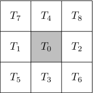
(a) Rectangular mesh

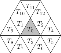
(b) Triangular mesh I

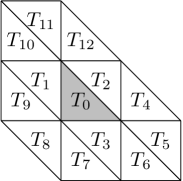
(c) Triangular mesh II

Figure 1: Labels of Moore neighbors.

Example 2.4 (rectangular meshes).

Next we consider a square mesh with spacing $h$ (Fig. 1(a)). The quadratic profile here takes the form

$$\begin{split}v_{h,0}^{n}(x,y)&=u_{0}+L_{x}(x-x_{0})+L_{y}(y-y_{0})+\dfrac{1}{2}H_{xx}(x-x_{0})^{2}+\dfrac{1}{2}H_{yy}(y-y_{0})^{2}\\ &+H_{xy}(x-x_{0})(y-y_{0})-\dfrac{1}{24}(H_{xx}+H_{yy})h^{2}.\end{split}$$

The optimal variables are $\bm{\varphi}=[hL_{x},hL_{y},h^{2}H_{xx}/2,h^{2}H_{xy},h^{2}H_{yy}/2]^{\top}$. And the coefficients of the objective function are

$$\mathbf{G}=\begin{bmatrix}6&&&&\\ &6&&&\\ &&6&&4\\ &&&4&\\ &&4&&6\end{bmatrix}\quad\text{~{}and~{}}\quad\bm{c}=-\begin{bmatrix}(u_{2}^{n}-u_{1}^{n})+(u_{6}^{n}-u_{5}^{n})+(u_{8}^{n}-u_{7}^{n})\\ (u_{4}^{n}-u_{3}^{n})+(u_{7}^{n}-u_{5}^{n})+(u_{8}^{n}-u_{6}^{n})\\ u_{1}^{n}+u_{2}^{n}+u_{5}^{n}+u_{6}^{n}+u_{7}^{n}+u_{8}^{n}-6u_{0}^{n}\\ (u_{5}^{n}+u_{8}^{n})-(u_{6}^{n}+u_{7}^{n})\\ u_{3}^{n}+u_{4}^{n}+u_{5}^{n}+u_{6}^{n}+u_{7}^{n}+u_{8}^{n}-6u_{0}^{n}\end{bmatrix}.$$

Example 2.5 (triangular meshes).

Here we use two special cases to illustrate the triangular meshes: the equilateral triangular mesh (Fig. 1(b)) and the diagonal triangular mesh (Fig. 1(c)). Choose $h$ to be the minimum side of the triangles. A simple calculation yields the following expression of $\mathbf{G}$:

$$\dfrac{1}{24}\begin{bmatrix}132&0&0&-14\sqrt{3}&0\\ 0&132&-14\sqrt{3}&0&14\sqrt{3}\\ 0&-14\sqrt{3}&105&0&35\\ -14\sqrt{3}&0&0&35&0\\ 0&14\sqrt{3}&35&0&105\end{bmatrix}\quad\text{~{}and~{}}\quad\dfrac{1}{9}\begin{bmatrix}66&-33&14&-7&-7\\ -33&66&-7&-7&14\\ 14&-7&70&-35&35\\ -7&-7&-35&35&-35\\ -7&14&35&-35&70\end{bmatrix}.$$

From this example we can expect that the matrix $\mathbf{G}$ is far from singularity for most triangular meshes.

The main computation cost of the integrated quadratic reconstruction is the solution of quadratic programming problems (15). An efficient and robust quadratic programming solver becomes essential. Here we use the active-set method [36] to solve the problem (14). This method updates the solution by solving a series of quadratic programming problems in which some of the inequalities are imposed as equalities. We repeatedly estimate the active set until the solution reaches optimality. To be more specific, let $\bm{\varphi}_{k}$ be solution of the $k$-th iterative step, then the descending direction $\bm{p}_{k}$ and Lagrange multipliers $\bm{\lambda}_{k}$ can be found by successively solving the following two linear systems

$$(\mathbf{M}\mathbf{G}^{-1}\mathbf{M}^{\top})\bm{\lambda}_{k} =\mathbf{M}(\bm{\varphi}_{k}+\mathbf{G}^{-1}\bm{c}),$$

$$\mathbf{G}\bm{p}_{k} =\mathbf{M}^{\top}\bm{\lambda}-\mathbf{G}\bm{\varphi}_{k}-\bm{c},$$

where the rows of matrix $\mathbf{M}$ are composed of normals of the active constraints at the current step. For a nonzero descending direction $\bm{p}_{k}$, we set $\bm{\varphi}_{k+1}=\bm{\varphi}_{k}+\alpha_{k}\bm{p}_{k}$. The step-length parameter $\alpha_{k}$ is given by

$$\alpha_{k}:=\min\left\{1,\min_{l}\beta_{l}\right\},\quad\beta_{l}=\begin{cases}\dfrac{b_{l}-\bm{a}_{l}^{\top}\bm{\varphi}_{k}}{\bm{a}_{l}^{\top}\bm{p}_{k}},&\bm{a}_{l}^{\top}\bm{p}_{k}<0,\\ \dfrac{B_{l}-\bm{a}_{l}^{\top}\bm{\varphi}_{k}}{\bm{a}_{l}^{\top}\bm{p}_{k}},&\bm{a}_{l}^{\top}\bm{p}_{k}>0,\\ +\infty,&\bm{a}_{l}^{\top}\bm{p}_{k}=0,\end{cases}$$

where $\bm{a}_{l}^{\top}$, $b_{l}$ and $B_{l}$ represent the $l$-th rows of matrices $\mathbf{A}$, $\bm{b}$ and $\bm{B}$ respectively. On the other hand, if $\bm{p}_{k}=\bm{0}$, then we check the signs of Lagrange multipliers. We have achieved the optimality if all the multipliers are non-negative; otherwise, we can find a feasible direction by dropping the constraint with the most negative multiplier. The initial guess is simply taken as the null solution, i.e. $\bm{\varphi}_{0}=\bm{0}$.

With the operator $\mathcal{R}_{h}$ specified by the procedure above, the numerical scheme (4) is then closed, while it leads to only first-order temporal accuracy. To match the third-order spatial accuracy, we adopt the SSP Runge-Kutta methods [37], which is a multi-stage combination of (4). The whole discretization scheme then reads

$$\begin{cases}u_{h}^{*}=u_{h}^{n}+\Delta t_{n}\mathcal{L}(v_{h}^{*}),&\quad v_{h}^{*}=\mathcal{R}_{h}[u_{h}^{n},v_{h}^{n-1}],\\ u_{h}^{**}=\dfrac{3}{4}u_{h}^{n}+\dfrac{1}{4}\left(u_{h}^{*}+\Delta t_{n}\mathcal{L}(v_{h}^{**})\right),&\quad v_{h}^{**}=\mathcal{R}_{h}[u_{h}^{*},v_{h}^{*}],\\ u_{h}^{n+1}=\dfrac{1}{3}u_{h}^{n}+\dfrac{2}{3}\left(u_{h}^{**}+\Delta t_{n}\mathcal{L}(v_{h}^{n})\right),&\quad v_{h}^{n}=\mathcal{R}_{h}[u_{h}^{**},v_{h}^{**}].\end{cases}$$

And the initial value of the SSP Runge-Kutta method is still given by (5).

3 Accuracy and Stability

In this section we study the accuracy and stability of the proposed scheme. Roughly speaking, the third-order temporal accuracy is provided by the SSP Runge-Kutta scheme already, thus we require a third-order spatial accuracy to achieve an overall third-order accuracy in the truncation error.

Basically, it can be shown that the quadratic reconstruction proposed above provides us a third-order spatial accuracy for smooth functions. To justify this point, we need to study the asymptotic behavior of the quadratic programming problem used to define the operator $\mathcal{R}_{h}$. In fact, let $\mathcal{P}_{h}=\{T_{i}\}_{i\in S}$ be a family of cell patches, where the relative position of the cells are the same, and hence $\bm{r}_{i}\propto h$, $\mathbf{J}_{i}\propto h^{2}$, etc. For the sake of convenience, the position of centroid of $T_{0}$ is fixed. To derive the continuous limit of problem (14), we first study the asymptotic expansions of the coefficients. Obvious both $\mathbf{G}$ and $\mathbf{A}$ are scale-invariant. Concerning the other coefficients, we have the following lemma:

Lemma 3.1.

There exist scale-invariant tensors $\overline{\mathbf{c}}\in\mathbb{R}^{d\times d}$, $\overline{\overline{\mathbf{c}}}\in\mathbb{R}^{d\times d\times d}$, $\overline{\mathbf{b}},\overline{\mathbf{B}}\in\mathbb{R}^{(JQ+1)\times d}$ and $\overline{\overline{\mathbf{b}}},\overline{\overline{\mathbf{B}}}\in\mathbb{R}^{(JQ+1)\times d\times d}$ such that the following asymptotic expansions hold

$$\bm{c} =h\overline{\mathbf{c}}\cdot\nabla u(\bm{x}_{0})+h^{2}\overline{\overline{\mathbf{c}}}:\nabla\nabla u(\bm{x}_{0})+\mathcal{O}(h^{3}),$$ (17a)

$$\bm{b} =h\overline{\mathbf{b}}\cdot\nabla u(\bm{x}_{0})+h^{2}\overline{\overline{\mathbf{b}}}:\nabla\nabla u(\bm{x}_{0})+\mathcal{O}(h^{3}),$$ (17b)

$$\bm{B} =h\overline{\mathbf{B}}\cdot\nabla u(\bm{x}_{0})+h^{2}\overline{\overline{\mathbf{B}}}:\nabla\nabla u(\bm{x}_{0})+\mathcal{O}(h^{3}).$$ (17c)

Proof 3.2.

Here we investigate the asymptotic expansion (17a) of $\bm{c}$. The expansions of $\bm{b}$ and $\bm{B}$ can be analyzed in a similar manner. Note that the Taylor expansion of $u(\bm{x})$ about $\bm{x}_{0}$ gives

$$u(\bm{x})=u(\bm{x}_{0})+(\bm{x}-\bm{x}_{0})^{\top}\nabla u(\bm{x}_{0})+\dfrac{1}{2}(\bm{x}-\bm{x}_{0})^{\top}\nabla\nabla u(\bm{x}_{0})(\bm{x}-\bm{x}_{0})+\mathcal{O}(h^{3}).$$

Therefore, the cell averages can be expressed as

$$u_{0}=\mathchoice{{\vbox{\hbox{$\textstyle-$ }}\kern-7.83337pt}}{{\vbox{\hbox{$\scriptstyle-$ }}\kern-5.90005pt}}{{\vbox{\hbox{$\scriptscriptstyle-$ }}\kern-4.75003pt}}{{\vbox{\hbox{$\scriptscriptstyle-$ }}\kern-4.25003pt}}\!\int_{T_{0}}u(\bm{x})\mathrm{d}\bm{x}=u(\bm{x}_{0})+\dfrac{1}{2}\mathbf{J}_{0}:\nabla\nabla u(\bm{x}_{0})+\mathcal{O}(h^{3}),$$

$$u_{i}=\mathchoice{{\vbox{\hbox{$\textstyle-$ }}\kern-7.83337pt}}{{\vbox{\hbox{$\scriptstyle-$ }}\kern-5.90005pt}}{{\vbox{\hbox{$\scriptscriptstyle-$ }}\kern-4.75003pt}}{{\vbox{\hbox{$\scriptscriptstyle-$ }}\kern-4.25003pt}}\!\int_{T_{i}}u(\bm{x})\mathrm{d}\bm{x}=u(\bm{x}_{0})+\bm{r}_{i}\cdot\nabla u(\bm{x}_{0})+\dfrac{1}{2}(\bm{r}_{i}\otimes\bm{r}_{i}+\mathbf{J}_{i}):\nabla\nabla u(\bm{x}_{0})+\mathcal{O}(h^{3}),$$

and as a result,

$$u_{i}-u_{0}=\bm{r}_{i}\cdot\nabla u(\bm{x}_{0})+\dfrac{1}{2}(\bm{r}_{i}\otimes\bm{r}_{i}+\mathbf{J}_{i}-\mathbf{J}_{0}):\nabla\nabla u(\bm{x}_{0})+\mathcal{O}(h^{3}).$$

The first-order coefficient then satisfies

$$\begin{split}\bm{c}&=-\sum_{i\in S}\bm{s}_{i}(u_{i}-u_{0})\\ &=-\sum_{i\in S}\bm{s}_{i}\left(\bm{r}_{i}\cdot\nabla u(\bm{x}_{0})+\dfrac{1}{2}(\bm{r}_{i}\otimes\bm{r}_{i}+\mathbf{J}_{i}-\mathbf{J}_{0}):\nabla\nabla u(\bm{x}_{0})\right)+\mathcal{O}(h^{3})\\ &=-\sum_{i\in S}(\bm{s}_{i}\otimes\bm{r}_{i})\cdot\nabla u(\bm{x}_{0})-\dfrac{1}{2}\sum_{i\in S}(\bm{s}_{i}\otimes(\bm{r}_{i}\otimes\bm{r}_{i}+\mathbf{J}_{i}-\mathbf{J}_{0})):\nabla\nabla u(\bm{x}_{0})+\mathcal{O}(h^{3}).\end{split}$$

From here we can identify the expansion coefficients $\overline{\mathbf{c}}$ and $\overline{\overline{\mathbf{c}}}$ in (17a).

With the aid of expansions (17), we are able to derive the continuous limit of the quadratic programming problem (14). Indeed, introduce a new variable $\bm{\psi}=\bm{\varphi}/h$, then the problem (14) can be turned into the following equivalent form

$$\begin{split}\min~{}&\dfrac{1}{2}\bm{\psi}^{\top}\mathbf{G}\bm{\psi}+h^{-1}\bm{c}^{\top}\bm{\psi}\\ \operatorname{s.t.}~{}&h^{-1}\bm{b}\leq\mathbf{A}\bm{\psi}\leq h^{-1}\bm{B}.\end{split}$$

From here we can see that the continuous limit of the problem (14) is

$$\begin{split}\min~{}&\dfrac{1}{2}\bm{\psi}^{\top}\mathbf{G}\bm{\psi}+(\overline{\mathbf{c}}\cdot\nabla u(\bm{x}_{0}))^{\top}\bm{\psi}\\ \operatorname{s.t.}~{}&\overline{\mathbf{b}}\cdot\nabla u(\bm{x}_{0})\leq\mathbf{A}\bm{\psi}\leq\overline{\mathbf{B}}\cdot\nabla u(\bm{x}_{0}).\end{split}$$ (18)

The above limiting problem provides us a precise statement of the well-posedness of the problem (14), which is a prerequisite of the accuracy result stated below.

Theorem 3.3.

Suppose that the solution operator $\mathcal{Q}(\mathbf{G},\cdot,\mathbf{A},\cdot,\cdot)$ is Lipschitz continuous in the neighborhood of $(\overline{\mathbf{c}}\cdot\nabla u(\bm{x}_{0}),~{}\overline{\mathbf{b}}\cdot\nabla u(\bm{x}_{0}),~{}\overline{\mathbf{B}}\cdot\nabla u(\bm{x}_{0}))$, then for any function $u\in C^{3}(\Omega)\bigcap L^{1}(\Omega)$, we have

$$\|\mathcal{R}_{h}[u]-u\|_{Z_{0}}=\mathcal{O}(h^{3}),$$

where the semi-norm $\|\cdot\|_{Z_{0}}$ is defined by $\|f\|_{Z_{0}}=\max_{\bm{z}\in Z_{0}}|f(\bm{z})|$.

Proof 3.4.

Denote the second-order Taylor polynomial of $u$ by

$$q(\bm{x})=u(\bm{x}_{0})+(\bm{x}-\bm{x}_{0})^{\top}\nabla u(\bm{x}_{0})+\dfrac{1}{2}(\bm{x}-\bm{x}_{0})^{\top}\nabla\nabla u(\bm{x}_{0})(\bm{x}-\bm{x}_{0}).$$

Obviously

$$\mathcal{R}_{h}[q]=q\quad\text{~{}and~{}}\quad\|q-u\|_{Z_{0}}=\mathcal{O}(h^{3}).$$

Then by the triangle inequality, we have

$$\begin{split}&\|\mathcal{R}_{h}[u]-u\|_{Z_{0}}\\ \leq&\|q-u\|_{Z_{0}}+\|\mathcal{R}_{h}[q]-q\|_{Z_{0}}+\|\mathcal{R}_{h}[u]-\mathcal{R}_{h}[q]\|_{Z_{0}}\\ \leq&\mathcal{O}(h^{3})+\mathcal{O}(h^{3})+\max_{\bm{z}\in Z_{0}}\|\bm{a}(\bm{z})\|\cdot\bigg{\|}h\mathcal{Q}\left({\mathbf{G}},h^{-1}\bm{c},{\mathbf{A}},h^{-1}\bm{b},h^{-1}\bm{B}\right)-h\mathcal{Q}\Big{(}{\mathbf{G}},\overline{\mathbf{c}}\cdot\nabla u(\bm{x}_{0})\\ +&h\overline{\overline{\mathbf{c}}}:\nabla\nabla u(\bm{x}_{0}),{\mathbf{A}},\overline{\mathbf{b}}\cdot\nabla u(\bm{x}_{0})+h\overline{\overline{\mathbf{b}}}:\nabla\nabla u(\bm{x}_{0}),\overline{\mathbf{B}}\cdot\nabla u(\bm{x}_{0})+h\overline{\overline{\mathbf{B}}}:\nabla\nabla u(\bm{x}_{0})\Big{)}\bigg{\|}\\ =&\mathcal{O}(h^{3})+\mathcal{O}(h)\cdot\mathcal{O}(h^{2})\\ =&\mathcal{O}(h^{3}).\end{split}$$

Of course this estimation is only valid for smooth functions. For conservation laws, solutions are so seldom to be smooth that the stability of the numerical scheme is of one’s more concern. High-order reconstruction may introduce spurious oscillations near discontinuities. One needs some stability criterion, such as the local maximum principle, to rule out solutions with spurious oscillations. Here we show that the forward Euler scheme (2) with our reconstruction satisfies a local maximum principle. The third-order SSP discretization will thereby satisfy the local maximum principle due to the convex combination.

Before verifying the local maximum principle, let us investigate the decomposition of the second moment tensor for an arbitrary control volume, as is stated in the following lemma:

Lemma 3.5.

Let $K_{j}$ be the $d$-dimensional hyper-pyramid formed by the centroid $\bm{x}_{0}$ of $T_{0}$ and its facet $e_{j}~{}(j=1,\cdots,J)$. Introduce the coefficients $\alpha_{j}=|K_{j}|/|T_{0}|~{}(j=1,\cdots,J)$. Then the following decomposition formula for the second moment tensor holds

$$\mathchoice{{\vbox{\hbox{$\textstyle-$ }}\kern-7.83337pt}}{{\vbox{\hbox{$\scriptstyle-$ }}\kern-5.90005pt}}{{\vbox{\hbox{$\scriptscriptstyle-$ }}\kern-4.75003pt}}{{\vbox{\hbox{$\scriptscriptstyle-$ }}\kern-4.25003pt}}\!\int_{T_{0}}\bm{x}\otimes\bm{x}\mathrm{d}\bm{x}=\dfrac{d}{d+2}\sum_{j=1}^{J}\alpha_{j}\mathchoice{{\vbox{\hbox{$\textstyle-$ }}\kern-7.83337pt}}{{\vbox{\hbox{$\scriptstyle-$ }}\kern-5.90005pt}}{{\vbox{\hbox{$\scriptscriptstyle-$ }}\kern-4.75003pt}}{{\vbox{\hbox{$\scriptscriptstyle-$ }}\kern-4.25003pt}}\!\int_{e_{j}}\bm{x}\otimes\bm{x}\mathrm{d}\bm{x}+\dfrac{2}{d+2}\bm{x}_{0}\otimes\bm{x}_{0}.$$

Proof 3.6.

At first, let us prove for any positive exponent $k$. One observes that

$$\mathchoice{{\vbox{\hbox{$\textstyle-$ }}\kern-7.83337pt}}{{\vbox{\hbox{$\scriptstyle-$ }}\kern-5.90005pt}}{{\vbox{\hbox{$\scriptscriptstyle-$ }}\kern-4.75003pt}}{{\vbox{\hbox{$\scriptscriptstyle-$ }}\kern-4.25003pt}}\!\int_{T_{0}}(\bm{x}-\bm{x}_{0})^{\otimes k}\mathrm{d}\bm{x}=\sum_{j=1}^{J}\alpha_{j}\mathchoice{{\vbox{\hbox{$\textstyle-$ }}\kern-7.83337pt}}{{\vbox{\hbox{$\scriptstyle-$ }}\kern-5.90005pt}}{{\vbox{\hbox{$\scriptscriptstyle-$ }}\kern-4.75003pt}}{{\vbox{\hbox{$\scriptscriptstyle-$ }}\kern-4.25003pt}}\!\int_{K_{j}}(\bm{x}-\bm{x}_{0})^{\otimes k}\mathrm{d}\bm{x}=\dfrac{d}{d+k}\sum_{j=1}^{J}\alpha_{j}\mathchoice{{\vbox{\hbox{$\textstyle-$ }}\kern-7.83337pt}}{{\vbox{\hbox{$\scriptstyle-$ }}\kern-5.90005pt}}{{\vbox{\hbox{$\scriptscriptstyle-$ }}\kern-4.75003pt}}{{\vbox{\hbox{$\scriptscriptstyle-$ }}\kern-4.25003pt}}\!\int_{e_{j}}(\bm{x}-\bm{x}_{0})^{\otimes k}\mathrm{d}\bm{x},$$ (19)

where $\bm{x}^{\otimes k}$ denotes a tensor product of $\bm{x}$ by $k$ times to produce a $k$-th order tensor. Actually, the control volume $T_{0}$ is composed by a set of hyper-pyramids $K_{1},\cdots,K_{J}$, thus we have

$$\int_{T_{0}}(\bm{x}-\bm{x}_{0})^{\otimes k}\mathrm{d}\bm{x}=\sum_{j=1}^{J}\int_{K_{j}}(\bm{x}-\bm{x}_{0})^{\otimes k}\mathrm{d}\bm{x}.$$

By the geometry of the hyper-pyramid $K_{j}$, we have

$$\int_{K_{j}}(\bm{x}-\bm{x}_{0})^{\otimes k}\mathrm{d}\bm{x}=\int_{0}^{1}l_{j}\mathrm{d}\lambda\int_{\lambda e_{j}}(\bm{x}-\bm{x}_{0})^{\otimes k}\mathrm{d}\bm{x},$$ (20)

where $l_{j}$ is the height of $K_{j}$, and $\lambda e_{j}$ presents the cross section of hyper-pyramid $K_{j}$ parallel to the bottom surface $e_{j}$. The distance to the vertex is $\lambda l_{j}$, and $K_{j}$ is shown in the figure 2.

By a geometric similarity argument, we have

$$\int_{\lambda e_{j}}(\bm{x}-\bm{x}_{0})^{\otimes k}\mathrm{d}\bm{x}=\lambda^{d+k-1}\int_{e_{j}}(\bm{x}-\bm{x}_{0})^{\otimes k}\mathrm{d}\bm{x},$$

and we insert it into (20) to have

$$\int_{K_{j}}(\bm{x}-\bm{x}_{0})^{\otimes k}\mathrm{d}\bm{x}=\dfrac{l_{j}}{d+k}\int_{e_{j}}(\bm{x}-\bm{x}_{0})^{\otimes k}\mathrm{d}\bm{x}=\dfrac{d}{d+k}|K_{j}|\mathchoice{{\vbox{\hbox{$\textstyle-$ }}\kern-7.83337pt}}{{\vbox{\hbox{$\scriptstyle-$ }}\kern-5.90005pt}}{{\vbox{\hbox{$\scriptscriptstyle-$ }}\kern-4.75003pt}}{{\vbox{\hbox{$\scriptscriptstyle-$ }}\kern-4.25003pt}}\!\int_{e_{j}}(\bm{x}-\bm{x}_{0})^{\otimes k}\mathrm{d}\bm{x}.$$

At last, we have that

$$\int_{T_{0}}(\bm{x}-\bm{x}_{0})^{\otimes k}\mathrm{d}\bm{x}=\dfrac{d}{d+k}\sum_{j=1}^{J}\alpha_{j}|T_{0}|\mathchoice{{\vbox{\hbox{$\textstyle-$ }}\kern-7.83337pt}}{{\vbox{\hbox{$\scriptstyle-$ }}\kern-5.90005pt}}{{\vbox{\hbox{$\scriptscriptstyle-$ }}\kern-4.75003pt}}{{\vbox{\hbox{$\scriptscriptstyle-$ }}\kern-4.25003pt}}\!\int_{e_{j}}(\bm{x}-\bm{x}_{0})^{\otimes k}\mathrm{d}\bm{x}.$$

which prove (19).

Figure 2: hyper-pyramid $K_{j}$

In particular, we have

$$\mathchoice{{\vbox{\hbox{$\textstyle-$ }}\kern-7.83337pt}}{{\vbox{\hbox{$\scriptstyle-$ }}\kern-5.90005pt}}{{\vbox{\hbox{$\scriptscriptstyle-$ }}\kern-4.75003pt}}{{\vbox{\hbox{$\scriptscriptstyle-$ }}\kern-4.25003pt}}\!\int_{T_{0}}(\bm{x}-\bm{x}_{0})\otimes(\bm{x}-\bm{x}_{0})\mathrm{d}\bm{x} =\dfrac{d}{d+2}\sum_{j=1}^{J}\alpha_{j}\mathchoice{{\vbox{\hbox{$\textstyle-$ }}\kern-7.83337pt}}{{\vbox{\hbox{$\scriptstyle-$ }}\kern-5.90005pt}}{{\vbox{\hbox{$\scriptscriptstyle-$ }}\kern-4.75003pt}}{{\vbox{\hbox{$\scriptscriptstyle-$ }}\kern-4.25003pt}}\!\int_{e_{j}}(\bm{x}-\bm{x}_{0})\otimes(\bm{x}-\bm{x}_{0})\mathrm{d}\bm{x},$$

$$\bm{0}=\mathchoice{{\vbox{\hbox{$\textstyle-$ }}\kern-7.83337pt}}{{\vbox{\hbox{$\scriptstyle-$ }}\kern-5.90005pt}}{{\vbox{\hbox{$\scriptscriptstyle-$ }}\kern-4.75003pt}}{{\vbox{\hbox{$\scriptscriptstyle-$ }}\kern-4.25003pt}}\!\int_{T_{0}}(\bm{x}-\bm{x}_{0})\mathrm{d}\bm{x} =\dfrac{d}{d+1}\sum_{j=1}^{J}\alpha_{j}\mathchoice{{\vbox{\hbox{$\textstyle-$ }}\kern-7.83337pt}}{{\vbox{\hbox{$\scriptstyle-$ }}\kern-5.90005pt}}{{\vbox{\hbox{$\scriptscriptstyle-$ }}\kern-4.75003pt}}{{\vbox{\hbox{$\scriptscriptstyle-$ }}\kern-4.25003pt}}\!\int_{e_{j}}(\bm{x}-\bm{x}_{0})\mathrm{d}\bm{x}.$$

And as a result

$$\mathchoice{{\vbox{\hbox{$\textstyle-$ }}\kern-7.83337pt}}{{\vbox{\hbox{$\scriptstyle-$ }}\kern-5.90005pt}}{{\vbox{\hbox{$\scriptscriptstyle-$ }}\kern-4.75003pt}}{{\vbox{\hbox{$\scriptscriptstyle-$ }}\kern-4.25003pt}}\!\int_{T_{0}}(\bm{x}-\bm{x}_{0})\otimes(\bm{x}-\bm{x}_{0})\mathrm{d}\bm{x} =\dfrac{d}{d+2}\sum_{j=1}^{J}\alpha_{j}\mathchoice{{\vbox{\hbox{$\textstyle-$ }}\kern-7.83337pt}}{{\vbox{\hbox{$\scriptstyle-$ }}\kern-5.90005pt}}{{\vbox{\hbox{$\scriptscriptstyle-$ }}\kern-4.75003pt}}{{\vbox{\hbox{$\scriptscriptstyle-$ }}\kern-4.25003pt}}\!\int_{e_{j}}(\bm{x}-\bm{x}_{0})\otimes(\bm{x}-\bm{x}_{0})\mathrm{d}\bm{x},$$

$$\mathchoice{{\vbox{\hbox{$\textstyle-$ }}\kern-7.83337pt}}{{\vbox{\hbox{$\scriptstyle-$ }}\kern-5.90005pt}}{{\vbox{\hbox{$\scriptscriptstyle-$ }}\kern-4.75003pt}}{{\vbox{\hbox{$\scriptscriptstyle-$ }}\kern-4.25003pt}}\!\int_{T_{0}}(\bm{x}-\bm{x}_{0})\otimes\bm{x}_{0}\mathrm{d}\bm{x} =\dfrac{d}{d+2}\sum_{j=1}^{J}\alpha_{j}\mathchoice{{\vbox{\hbox{$\textstyle-$ }}\kern-7.83337pt}}{{\vbox{\hbox{$\scriptstyle-$ }}\kern-5.90005pt}}{{\vbox{\hbox{$\scriptscriptstyle-$ }}\kern-4.75003pt}}{{\vbox{\hbox{$\scriptscriptstyle-$ }}\kern-4.25003pt}}\!\int_{e_{j}}(\bm{x}-\bm{x}_{0})\otimes\bm{x}_{0}\mathrm{d}\bm{x},$$

$$\mathchoice{{\vbox{\hbox{$\textstyle-$ }}\kern-7.83337pt}}{{\vbox{\hbox{$\scriptstyle-$ }}\kern-5.90005pt}}{{\vbox{\hbox{$\scriptscriptstyle-$ }}\kern-4.75003pt}}{{\vbox{\hbox{$\scriptscriptstyle-$ }}\kern-4.25003pt}}\!\int_{T_{0}}\bm{x}_{0}\otimes(\bm{x}-\bm{x}_{0})\mathrm{d}\bm{x} =\dfrac{d}{d+2}\sum_{j=1}^{J}\alpha_{j}\mathchoice{{\vbox{\hbox{$\textstyle-$ }}\kern-7.83337pt}}{{\vbox{\hbox{$\scriptstyle-$ }}\kern-5.90005pt}}{{\vbox{\hbox{$\scriptscriptstyle-$ }}\kern-4.75003pt}}{{\vbox{\hbox{$\scriptscriptstyle-$ }}\kern-4.25003pt}}\!\int_{e_{j}}\bm{x}_{0}\otimes(\bm{x}-\bm{x}_{0})\mathrm{d}\bm{x},$$

$$\mathchoice{{\vbox{\hbox{$\textstyle-$ }}\kern-7.83337pt}}{{\vbox{\hbox{$\scriptstyle-$ }}\kern-5.90005pt}}{{\vbox{\hbox{$\scriptscriptstyle-$ }}\kern-4.75003pt}}{{\vbox{\hbox{$\scriptscriptstyle-$ }}\kern-4.25003pt}}\!\int_{T_{0}}\bm{x}_{0}\otimes\bm{x}_{0}\mathrm{d}\bm{x} =\dfrac{d}{d+2}\sum_{j=1}^{J}\alpha_{j}\mathchoice{{\vbox{\hbox{$\textstyle-$ }}\kern-7.83337pt}}{{\vbox{\hbox{$\scriptstyle-$ }}\kern-5.90005pt}}{{\vbox{\hbox{$\scriptscriptstyle-$ }}\kern-4.75003pt}}{{\vbox{\hbox{$\scriptscriptstyle-$ }}\kern-4.25003pt}}\!\int_{e_{j}}\bm{x}_{0}\otimes\bm{x}_{0}\mathrm{d}\bm{x}+\dfrac{2}{d+2}\bm{x}_{0}\otimes\bm{x}_{0}.$$

Summing up the above four identities yields the desired formula.

Next we can establish the following quadrature rule

Lemma 3.7.

The following quadrature formula is exact for any quadratic polynomial $v$

$$\mathchoice{{\vbox{\hbox{$\textstyle-$ }}\kern-7.83337pt}}{{\vbox{\hbox{$\scriptstyle-$ }}\kern-5.90005pt}}{{\vbox{\hbox{$\scriptscriptstyle-$ }}\kern-4.75003pt}}{{\vbox{\hbox{$\scriptscriptstyle-$ }}\kern-4.25003pt}}\!\int_{T_{0}}v(\bm{x})\mathrm{d}\bm{x}=\dfrac{d}{d+2}\sum_{j=1}^{J}\sum_{q=1}^{Q_{j}}\alpha_{j}w_{jq}v(\bm{z}_{jq})+\dfrac{2}{d+2}v(\bm{x}_{0}).$$ (21)

Proof 3.8.

Since the quadrature rules specified on the facet $e_{j}$ is of at least second-order accuracy, we have

$$\sum_{q=1}^{Q_{j}}w_{jq}\bm{z}_{jq}=\mathchoice{{\vbox{\hbox{$\textstyle-$ }}\kern-7.83337pt}}{{\vbox{\hbox{$\scriptstyle-$ }}\kern-5.90005pt}}{{\vbox{\hbox{$\scriptscriptstyle-$ }}\kern-4.75003pt}}{{\vbox{\hbox{$\scriptscriptstyle-$ }}\kern-4.25003pt}}\!\int_{e_{j}}\bm{x}\mathrm{d}\bm{x}\quad\text{~{}and~{}}\quad\sum_{q=1}^{Q_{j}}w_{jq}\bm{z}_{jq}\otimes\bm{z}_{jq}=\mathchoice{{\vbox{\hbox{$\textstyle-$ }}\kern-7.83337pt}}{{\vbox{\hbox{$\scriptstyle-$ }}\kern-5.90005pt}}{{\vbox{\hbox{$\scriptscriptstyle-$ }}\kern-4.75003pt}}{{\vbox{\hbox{$\scriptscriptstyle-$ }}\kern-4.25003pt}}\!\int_{e_{j}}\bm{x}\otimes\bm{x}\mathrm{d}\bm{x}.$$

Using the formula in Lemma 3.5 we know that

$$\dfrac{d}{d+2}\sum_{j=1}^{J}\sum_{q=1}^{Q_{j}}\alpha_{j}w_{jq}\bm{z}_{jq}+\dfrac{2}{d+2}\bm{x}_{0}=\bm{x}_{0}=\mathchoice{{\vbox{\hbox{$\textstyle-$ }}\kern-7.83337pt}}{{\vbox{\hbox{$\scriptstyle-$ }}\kern-5.90005pt}}{{\vbox{\hbox{$\scriptscriptstyle-$ }}\kern-4.75003pt}}{{\vbox{\hbox{$\scriptscriptstyle-$ }}\kern-4.25003pt}}\!\int_{T_{0}}\bm{x}\mathrm{d}\bm{x},$$

$$\dfrac{d}{d+2}\sum_{j=1}^{J}\sum_{q=1}^{Q_{j}}\alpha_{j}w_{jq}\bm{z}_{jq}\otimes\bm{z}_{jq}+\dfrac{2}{d+2}\bm{x}_{0}\otimes\bm{x}_{0}=\mathbf{J}_{0}+\bm{x}_{0}\otimes\bm{x}_{0}=\mathchoice{{\vbox{\hbox{$\textstyle-$ }}\kern-7.83337pt}}{{\vbox{\hbox{$\scriptstyle-$ }}\kern-5.90005pt}}{{\vbox{\hbox{$\scriptscriptstyle-$ }}\kern-4.75003pt}}{{\vbox{\hbox{$\scriptscriptstyle-$ }}\kern-4.25003pt}}\!\int_{T_{0}}\bm{x}\otimes\bm{x}\mathrm{d}\bm{x}.$$

From this we conclude that (21) holds for the function $v:\bm{x}\rightarrow\bm{x}$ and $v:\bm{x}\rightarrow\bm{x}\otimes\bm{x}$, and so is any quadratic function $v$. This completes the proof.

With the aid of the formula (21), we are able to verify a local maximum principle for the finite volume scheme (2) following the line in [34].

Theorem 3.9.

Suppose that $\mathcal{T}$ is a convex $d$-polytope grid. Let $L_{\min}$ be the minimum distance from the centroid of any given cell to all the facets of this cell. Moreover, let $\mathcal{F}$ be a monotone $C^{1}$ numerical flux function. Then the finite volume scheme (2) with integrated quadratic reconstruction fulfills the following local maximum principle

$$\min_{0\leq j\leq J}\min_{\bm{z}\in Z_{j}}{v_{h,j}^{n}(\bm{z})}\leq u_{0}^{n+1}\leq\max_{0\leq j\leq J}\max_{\bm{z}\in Z_{j}}{v_{h,j}^{n}(\bm{z})},$$ (22)

under the CFL condition

$$\Delta t_{n}\sup_{u^{-},u^{+},\bm{n}}\dfrac{\partial\mathcal{F}(u^{-},u^{+};\bm{n})}{\partial u^{-}}\leq\dfrac{L_{\min}}{d+2}.$$ (23)

Proof 3.10.

Inserting the quadrature formula (21) into the finite volume scheme (2) yields

$$u_{0}^{n+1}=\dfrac{2}{d+2}v_{h,0}^{n}(\bm{x}_{0})+\sum_{j=1}^{J}\sum_{q=1}^{Q_{j}}\left(\dfrac{d\alpha_{j}}{d+2}w_{jq}v_{h,0}^{n}(\bm{z}_{jq})-\dfrac{\Delta t_{n}}{|T_{0}|}w_{jq}\mathcal{F}(v_{h,0}^{n}(\bm{z}_{jq}),v_{h,j}^{n}(\bm{z}_{jq});\bm{n}_{j})|e_{j}|\right),$$

If we take the right-hand side of the above scheme as a function

$$u_{0}^{n+1}=\mathcal{H}(v_{h,0}^{n}(\bm{z}_{11}),\cdots,v_{h,0}^{n}(\bm{z}_{JQ_{J}}),v_{h,1}^{n}(\bm{z}_{11}),\cdots,v_{h,J}^{n}(\bm{z}_{JQ_{J}}),v_{h,0}^{n}(\bm{x}_{0})),$$

we then have that

$$\dfrac{\partial\mathcal{H}}{\partial v_{h,0}^{n}(\bm{z}_{jq})} =\dfrac{d\alpha_{j}w_{jq}}{d+2}-\dfrac{\Delta t_{n}|e_{j}|w_{jq}}{|T_{0}|}\cdot\dfrac{\partial\mathcal{F}(v_{h,0}^{n}(\bm{z}_{jq}),v_{h,j}^{n}(\bm{z}_{jq});\bm{n}_{j})}{\partial v_{h,0}^{n}(\bm{z}_{jq})}$$

$$\geq\dfrac{d\alpha_{j}w_{jq}}{d+2}-\dfrac{\Delta t_{n}|e_{j}|w_{jq}}{|T_{0}|}\sup_{u^{-},u^{+},\bm{n}}\dfrac{\partial\mathcal{F}(u^{-},u^{+};\bm{n})}{\partial u^{-}},$$

$$\dfrac{\partial\mathcal{H}}{\partial v_{h,j}^{n}(\bm{z}_{jq})} =-\dfrac{\Delta t_{n}|e_{j}|w_{jq}}{|T_{0}|}\cdot\dfrac{\partial\mathcal{F}(v_{h,0}^{n}(\bm{z}_{jq}),v_{h,j}^{n}(\bm{z}_{jq});\bm{n}_{j})}{\partial v_{h,j}^{n}(\bm{z}_{jq})}\geq 0,$$

$$\dfrac{\partial\mathcal{H}}{\partial v_{h,0}^{n}(\bm{x}_{0})} =\dfrac{2}{d+2}>0.$$

As a result, $\mathcal{H}$ is non-decreasing with respect to each argument provided that

$$\Delta t_{n}\sup_{u^{-},u^{+},\bm{n}}\dfrac{\partial\mathcal{F}(u^{-},u^{+};\bm{n})}{\partial u^{-}}\leq\dfrac{d}{d+2}\min_{1\leq j\leq J}\dfrac{\alpha_{j}|T_{0}|}{|e_{j}|}=\dfrac{1}{d+2}\min_{1\leq j\leq J}\dfrac{d|K_{j}|}{|e_{j}|}.$$

Note that $d|K_{j}|/|e_{j}|$ is exactly the distance from the point $\bm{x}_{0}$ to the facet $e_{j}$. Therefore, a sufficient condition of the time restriction is

$$\Delta t_{n}\sup_{u^{-},u^{+},\bm{n}}\dfrac{\partial\mathcal{F}(u^{-},u^{+};\bm{n})}{\partial u^{-}}\leq\dfrac{L_{\min}}{d+2}.$$

Also, we have $\mathcal{H}(u,\cdots,u)=u$ due to the consistency of numerical flux functions. Denote

$$u^{\min}=\min_{0\leq j\leq J}\min_{\bm{z}\in Z_{j}}{v_{h,j}^{n}(\bm{z})}\quad\text{~{}and~{}}\quad u^{\max}=\max_{0\leq j\leq J}\max_{\bm{z}\in Z_{j}}{v_{h,j}^{n}(\bm{z})},$$

then the monotonicity of $\mathcal{H}$ implies the desired local maximum principle

$$u^{\min}\leq\mathcal{H}(u^{\min},\cdots,u^{\min})\leq u_{0}^{n+1}\leq\mathcal{H}(u^{\max},\cdots,u^{\max})=u^{\max}.$$

Remark 3.11.

Another form of CFL condition in terms of the mesh size $h$ is also useful

$$a\Delta t_{n}\leq\nu h,$$

where $\nu$ is a CFL number. Here we measure the mesh size $h$ of simplicial control volume (triangle or tetrahedron) by the diameter of its inscribed ball, whereas that of Cartesian control volume (rectangle or cuboid) the harmonic mean of its dimensions. The value of CFL number $\nu$ under such definition is also listed in Table 1.

Although the local maximum principle given in Theorem 3.9 is not recursively formulated, we can verify the bound-preserving property, saying the numerical solution at any time level is bounded by the initial solution. More specifically, we have

Corollary 3.12.

The finite volume scheme (2) with integrated quadratic reconstruction is bound-preserving, namely

$$\inf_{\bm{x}\in\Omega}{u(\bm{x},0)}\leq u_{0}^{n}\leq\sup_{\bm{x}\in\Omega}{u(\bm{x},0)},$$ (24)

provided that the solution is advanced with a time step subjected to the CFL condition (23).

Proof 3.13.

Introduce the following notations of global upper bounds at $n$-th time level

$$M^{n}=\max_{T_{0}\in\mathcal{T}}{u_{0}^{n}},\quad\hat{M}^{n}=\max_{T_{0}\in\mathcal{T}}\max_{\bm{z}\in Z_{0}}{v_{h,0}^{n}(\bm{z})},\quad n=0,1,2,\cdots.$$

Since $u_{0}^{n}$ is a convex combination of $\{v_{h,0}^{n}(\bm{z})\}_{\bm{z}\in Z_{0}}$, we have $u_{0}^{n}\leq\max\limits_{\bm{z}\in Z_{0}}{v_{h,0}^{n}(\bm{z})}$. Taking the maximum over all $T_{0}\in\mathcal{T}$ yields the relation $M^{n}\leq\hat{M}^{n}$. For any cell $T_{0}\in\mathcal{T}$ and $\bm{z}\in Z_{0}$, the construction of integrated quadratic reconstruction yields

$$v_{h,0}^{n}(\bm{z})\leq\max\limits_{0\leq j\leq J}{M_{0j}^{n}}\leq\max\{\hat{M}^{n-1},M^{n}\},\quad\forall\bm{z}\in Z_{0},$$

and hence $\hat{M}^{n}\leq\max\{\hat{M}^{n-1},M^{n}\}$. Note that the local maximum principle (22) implies that $M^{n}\leq\hat{M}^{n-1}$. Therefore we have the monotonicity

$$\hat{M}^{n}\leq\hat{M}^{n-1},\quad n=1,2,\cdots.$$

On the other hand, the construction of initial time level yields

$$v_{h,0}^{0}(\bm{z})\leq\max\limits_{0\leq j\leq J}{M_{0j}^{0}}\leq\max\left\{\max_{T_{0}\in\mathcal{T}}\max_{\bm{z}\in Z_{0}}u(\bm{z},0),M^{0}\right\}\leq\sup_{\bm{x}\in\Omega}{u(\bm{x},0)},\quad\forall\bm{z}\in Z_{0},$$

and hence $\hat{M}^{0}\leq\sup\limits_{\bm{x}\in\Omega}{u(\bm{x},0)}$. Finally we conclude that

$$u_{0}^{n}\leq M^{n}\leq\hat{M}^{n}\leq\cdots\leq\hat{M}^{0}\leq\sup\limits_{\bm{x}\in\Omega}{u(\bm{x},0)}.$$

Similarly we can verify the left-hand side of the inequality (24).

4 Numerical Results

In this section we provide some numerical results to demonstrate the performance of the integrated quadratic reconstruction. The time step length is indicated by the CFL number listed in Table 1 if not otherwise specified. The results are compared against the scaling limiter of Zhang et al. [34] acting on the 2-exact reconstruction, which we refer to as the scaling quadratic reconstruction (SQR) in our context.

4.1 Two-dimensional linear equation

This is a two-dimensional problem used to assess the order of accuracy. We solve the following linear equation

$$u_{t}+u_{x}+2u_{y}=0,$$

with initial profile given by the double sine wave function

$$u(x,y,0)=\sin(2\pi x)\sin(2\pi y).$$

This problem has also been considered in [25, 26, 38, 27]. The computational domain is $[0,1]\times[0,1]$. Periodic boundary conditions are applied. We perform the convergence test on both rectangular and triangular meshes. The rectangular mesh is uniform. In the triangular mesh test, both structured and unstructured meshes are examined. The structured mesh is generated by dividing each rectangular element along the diagonal direction, while the unstructured mesh is generated by Delaunay triangulation. In Table 4.1, one observes third-order of accuracy on various meshes.

tableAccuracy for 2D linear equation.    Rectangular meshes $h$ $L^{1}$ error Order $L^{\infty}$ error Order $1/8$ 3.84E-01 — 9.52E-01 — $1/16$ 1.36E-01 1.50 3.38E-01 1.50 $1/32$ 2.08E-02 2.71 5.34E-02 2.66 $1/64$ 2.68E-03 2.96 7.44E-03 2.84 $1/128$ 3.37E-04 3.00 1.09E-03 2.77 $1/256$ 4.21E-05 3.00 1.79E-04 2.60    Structured triangular meshes $h$ $L^{1}$ error Order $L^{\infty}$ error Order $1/8$ 2.79E-01 — 5.14E-01 — $1/16$ 7.22E-02 1.95 1.27E-01 2.02 $1/32$ 1.02E-02 2.82 1.82E-02 2.80 $1/64$ 1.30E-03 2.97 2.54E-03 2.84 $1/128$ 1.63E-04 3.00 3.75E-04 2.76 $1/256$ 2.04E-05 3.00 6.22E-05 2.59    Unstructured triangular meshes $h$ $L^{1}$ error Order $L^{\infty}$ error Order $1/5$ 3.40E-01 — 8.24E-01 — $1/10$ 1.05E-01 1.69 2.41E-01 1.78 $1/20$ 1.58E-02 2.73 3.85E-02 2.64 $1/40$ 2.05E-03 2.95 5.63E-03 2.77 $1/80$ 2.59E-04 2.99 9.84E-04 2.52 $1/160$ 3.25E-05 2.99 2.00E-04 2.30

4.2 Composite model problem

In this example we use a composite model problem to test the robustness of the proposed scheme. The following linear advection equation is computed

$$u_{t}+u_{x}+0u_{y}=0,$$

on the square domain $[0,1]\times[0,1]$. The initial profile consists of two bulks with large discrepancy in magnitude, i.e.

$$u(x,y,0)=\begin{cases}A,&1/8\leq x\leq 3/8\text{~{}and~{}}3/8\leq y\leq 5/8,\\ 100,&5/8\leq x\leq 7/8\text{~{}and~{}}3/8\leq y\leq 5/8,\\ 0,&\text{Otherwise}.\end{cases}$$

where $A=1$ or $10$ denotes the magnitude of the short bulk.

The solution of IQR and SQR schemes on a fine structured mesh at $t=0.1$ are shown in Fig. 4. Only the short bulk is displayed here for the sake of visibility. We would like to mention that the global range $[0,100]$ of the initial solution is required as a parameter in the SQR scheme. It is observed that the SQR scheme produces severe oscillation on the front edge of the short bulk, though the global range of the solution is strictly preserved within the interval $[0,100]$. To quantitatively study the behavior of the short bulk when the mesh is refined, we measure the peak value of the short bulk on successively refined meshes, as is shown in Table 2. It is observed that the amount of the overshoot is about $11\%$ the magnitude of the short bulk for the SQR scheme, regardless of the resolution of the numerical scheme. Indeed, due to the presence of the tall bulk, the scaling limiter makes no difference to the edge of the short bulk. On the other hand, the IQR scheme maintains the range of the short bulk due to its locality and parameter-free performance. From this perspective we confirm the robustness of the IQR scheme.

Figure 3: Compositor Model Problem

(a) IQR

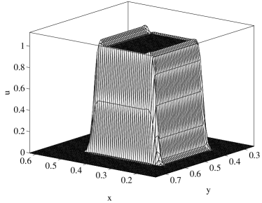
(b) SQR

Figure 4: Shape of the short bulk at $t=0.1$ with $128\times 128\times 2$ cells.

Table 2: Peak value of the short bulk at $t=0.1$ on successively refined meshes.

	$A=1$			$A=10$
$h$	SQR	IQR		SQR	IQR
$1/16$	1.1441	1.0000		11.4405	10.0000
$1/32$	1.1535	1.0000		11.5353	10.0000
$1/64$	1.1268	1.0000		11.2681	10.0000
$1/128$	1.1298	1.0000		11.2984	10.0000

4.3 Solid body rotation problem

This is a non-uniform scalar flow where the initial profile consists of smooth hump, cone and slotted cylinder. See [39] for the algebraic descriptions of the geometric shapes. We solve the circular advection equation

$$u_{t}-(y-0.5)u_{x}+(x-0.5)u_{y}=0,$$

on $[0,1]\times[0,1]$ with homogeneous boundary conditions. Fig. 5 shows the results after one revolution on two levels of Delaunay meshes. In the finer mesh, the IQR scheme almost keeps the shape of the initial solution without much distortion.

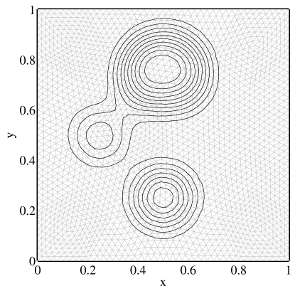
(a)

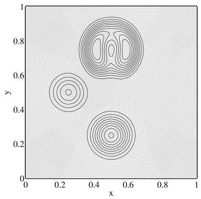
(b)

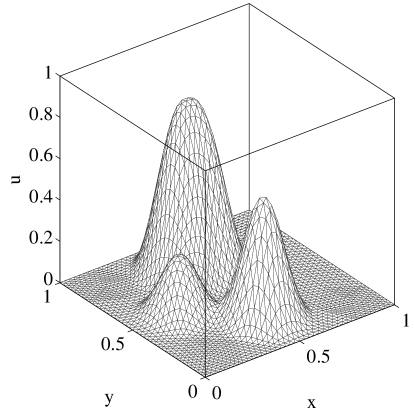
(c)

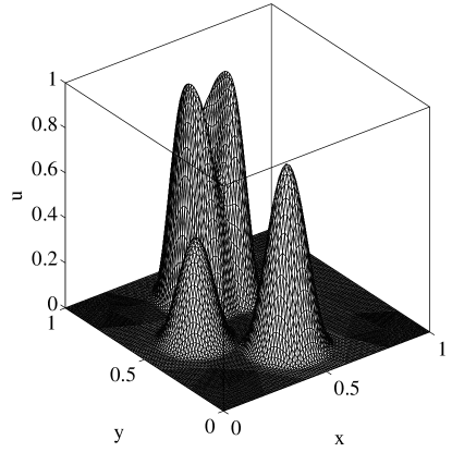
(d)

Figure 5: Solutions of the solid body rotation problem at $t=2\pi$: left panel (4096 cells) and right panel (16384 cells).

4.4 Two-dimensional Burgers’ equation

Following [13], we consider the two-dimensional Burgers’ equation

$$u_{t}+\left(\dfrac{1}{2}u^{2}\right)_{x}+\left(\dfrac{1}{2}u^{2}\right)_{y}=0,$$ (25)

with initial condition $u(x,y,0)=0.3+0.7\sin({\pi}(x+y)/2)$ on the domain $[-2,2]\times[-2,2]$. Periodic boundary conditions are applied. To assess the order of accuracy on smooth regions we advance the solution until $t=0.5/\pi^{2}$. The exact solution at a given position $(x,y)$ can be found by applying a fixed-point iteration to the nonlinear algebraic equation

$$u=0.3+0.7\sin\left(\dfrac{\pi}{2}(x+y)-\dfrac{u}{2\pi}\right).$$

The underlying meshes we use here are the same as that of Figs. 3.2 and 3.3 in Hu and Shu [13]. The accuracy results of both IQR and SQR schemes are listed in Tables 3 and 4. A third-order accuracy is maintained for both structured and unstructured meshes.

Table 3: Accuracy of 2D Burgers’ equation at $t=0.5/\pi^{2}$ on structured grids

IQR						SQR
$h$	$L^{1}$ error	Order	$L^{\infty}$ error	Order		$L^{1}$ error	Order	$L^{\infty}$ error	Order
$2/5$	3.38E-01	—	6.63E-02	—		4.16E-01	—	6.72E-02	—
$1/5$	4.54E-02	2.89	9.89E-03	2.75		4.54E-02	3.20	9.89E-03	2.76
$1/10$	5.73E-03	2.99	1.31E-03	2.92		5.73E-03	2.99	1.31E-03	2.92
$1/20$	7.21E-04	2.99	1.67E-04	2.98		7.21E-04	2.99	1.67E-04	2.98
$1/40$	9.14E-05	2.98	2.09E-05	2.99		9.01E-05	3.00	2.09E-05	2.99

Table 4: Accuracy of 2D Burgers’ equation at $t=0.5/\pi^{2}$ on unstructured grids

IQR						SQR
$h$	$L^{1}$ error	Order	$L^{\infty}$ error	Order		$L^{1}$ error	Order	$L^{\infty}$ error	Order
$1/2$	2.28E-01	—	7.59E-02	—		2.27E-01	—	7.59E-02	—
$1/4$	3.02E-02	2.92	1.18E-02	2.68		3.01E-02	2.91	1.18E-02	2.68
$1/8$	3.81E-03	2.99	1.66E-03	2.84		3.80E-03	2.98	1.66E-03	2.84
$1/16$	4.80E-04	2.99	2.19E-04	2.92		4.76E-04	3.00	2.19E-04	2.92
$1/32$	6.08E-05	2.98	2.82E-05	2.96		5.94E-05	3.00	2.82E-05	2.96

To demonstrate the application for shock computations we compute until $t=5/\pi^{2}$. Fig. 6 shows the results for a structured mesh with $h=1/20$ and an unstructured mesh with $h=1/16$, following the resolution that was used in [13]. From here we can see that the shock front, located on $x+y=3/\pi^{2}\pm 2$, is captured well.

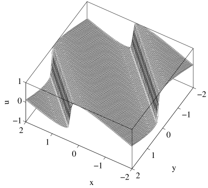
(a) Structured mesh: $h=1/20$

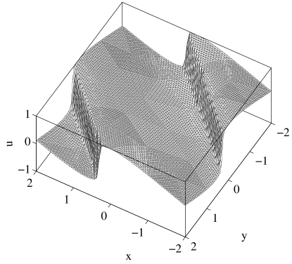
(b) Unstructured mesh: $h=1/16$

Figure 6: Solution of 2D Burgers’ equation at $t=5/\pi^{2}$.

4.5 Two-dimensional Riemann problem

To investigate the performance of IQR scheme in the presence of genuinely multi-dimensional nonlinear waves, we solve the Riemann problem [40] of Burgers’ equations (25)

$$u(x,y,0)=\begin{cases}2,&x,y<0.25,\\ 3,&x,y>0.25,\\ 1,&\text{Otherwise},\end{cases}$$

on the domain $[0,1]\times[0,1]$. Inflow boundary conditions are prescribed at the left and bottom edges of the boundary to mimic the motion of shocks. Two shock waves and two rarefactions will meet towards the center of the domain to form a double-parabola-shaped cusp. In our computation the solution is advanced to $t=1/12$. The exact solution can be found by using the method of characteristics, i.e.

$$u(x,y,t)=\begin{cases}3,&\min\{x,y\}>0.25+3t,\\ (\min\{x,y\}\!-\!0.25)/t,&0.25+2t-\min\{\sqrt{2|x-y|t},t\}\leq\min\{x,y\}\leq 0.25+3t,\\ 1,&\min\{x,y\}<0.25+t\leq 0.25+1.5t<\max\{x,y\},\\ 2,&\text{Otherwise}.\end{cases}$$

On successively refined Delaunay meshes, the $L^{1}$ errors at $t=1/12$ are shown in Fig. 7(a), with an order of accuracy close to one, which confirms that IQR scheme is genuinely high-order. The contour lines of the solution on a fine mesh are shown in Fig. 7(b). The result exhibits high resolution for the central cusp and shock front.

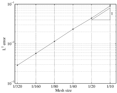
(a) $L^{1}$ error versus mesh size (first-order)

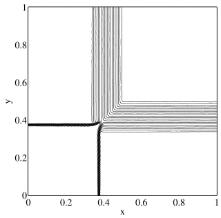
(b) Contour lines on the mesh $h=1/160$

Figure 7: Riemann problem of Burgers’ equation at $t=1/12$.

4.6 Three-dimensional linear equation

This is a three-dimensional problem used to assess the order of accuracy. We solve the following linear equation

$$u_{t}+u_{x}+u_{y}+u_{z}=0,$$

with initial profile given by the triple sine wave function

$$u(x,y,z,0)=\sin(2\pi x)\sin(2\pi y)\sin(2\pi z).$$

The computation domain is $[0,1]\times[0,1]\times[0,1]$. We perform the convergence test on unstructured tetrahedron mesh with periodic boundary condition applied. In Table 5, one observes third-order of accuracy on such kind mesh.

Table 5: Accuracy for 3D linear equation.

$h$	$L^{1}$ error	Order	$L^{\infty}$ error	Order
1/10	1.05E-01	—	7.59E-01	—
1/20	4.47E-02	2.03	1.86E-01	2.02
1/40	6.69E-03	2.66	2.61E-02	2.67
1/80	8.51E-04	2.80	3.46E-03	2.75

4.7 Three-dimensional Burgers’ equation

In this last test we compute the three-dimensional Burgers’ equation [18]

$$u_{t}+\left(\dfrac{1}{2}u^{2}\right)_{x}+\left(\dfrac{1}{2}u^{2}\right)_{y}+\left(\dfrac{1}{2}u^{2}\right)_{z}=0,$$

with initial data $u(x,y,z,0)=0.3+0.7\sin({\pi}(x+y+z)/3)$ on the cube domain $[-3,3]\times[-3,3]\times[-3,3]$ with periodic boundary conditions. The CFL number is taken as $0.1$ here. The convergence order at $t=0.5/\pi^{2}$ is listed in Table 6, where full accuracy is observed. We also present the contour plots of the solution at $t=5/\pi^{2}$ on the surface and the 2D slice $z=0$ as well as the 1D cutting-plot along the line $x=y,z=0$ in Fig 8. We can observe that the solution is non-oscillatory and the shock is resolved sharply.

Table 6: Accuracy for 3D Burgers’ equation.

$h$	$L^{1}$ error	Order	$L^{\infty}$ error	Order
$3/4$	1.42E+01	—	2.88E-01	—
$3/8$	2.17E+00	2.71	5.32E-02	2.44
$3/16$	2.85E-01	2.93	7.61E-03	2.81
$3/32$	3.59E-02	3.00	9.95E-04	2.94

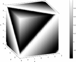
(a) Solution on the surface

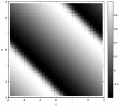
(b) Solution on the slice $z=0$

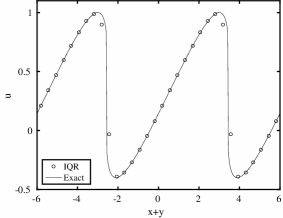
(c) Cutting-plot along $x=y$, $z=0$

Figure 8: Three-dimensional Burgers’ equation at $t=5/\pi^{2}$ with $32\times 32\times 32$ cells.

We remark that even a third-order accuracy is observed in the numerical examples, Theorem 1 does not guarantee the numerical solution a third-order accuracy since it depends on if the upper and the lower bound in the reconstruction have the same accuracy order. For multiple dimensional problems, it looks the third-order accuracy able to be preserved during the evolving of the scheme, while it is harder to preserve the accuracy order for one dimensional problem since the maximal value can be available at only one point.

5 Conclusion

We proposed an integrated quadratic reconstruction method for high-order finite volume schemes to scalar conservation laws in multiple dimensions. The reconstruction is applicable on flexible grids and requires no problem dependent parameters. Moreover, it gives us a finite volume scheme which satisfies a local maximum principle. Numerical results showed the accuracy and robustness of the proposed scheme. In the future, we are interested in how to extend the reconstruction strategy here to systems of conservation laws.

References

References

• [1] C. Michalak and C. Ollivier-Gooch. Accuracy preserving limiter for the high-order accurate solution of the Euler equations. Journal of Computational Physics, 228(23):8693–8711, 2009.
• [2] T.J. Barth and P.O. Frederickson. Higher order solution of the Euler equations on unstructured grids using quadratic reconstruction. In 28th AIAA Aerospace Sciences Meeting, 1990.
• [3] C.R. Mitchell and R.W. Walters. $k$-exact reconstruction for the Navier-Stokes equations on arbitrary grids. In 31st AIAA Aerospace Sciences Meeting, 1993.
• [4] T.J. Barth. Recent developments in high order $k$-exact reconstruction on unstructured meshes. In 31st AIAA Aerospace Sciences Meeting, 1993.
• [5] C. Ollivier-Gooch, A. Nejat, and K. Michalak. Obtaining and verifying high-order unstructured finite volume solutions to the Euler equations. AIAA Journal, 47(9):2105–2120, 2009.
• [6] W. Li and Y.X. Ren. High-order $k$-exact WENO finite volume schemes for solving gas dynamic Euler equations on unstructured grids. International Journal for Numerical Methods in Fluids, 70(6):742–763, 2012.
• [7] G. Hu and N. Yi. An adaptive finite volume solver for steady Euler equations with non-oscillatory $k$-exact reconstruction. Journal of Computational Physics, 312:235–251, 2016.
• [8] Y. Liu, C.-W. Shu, E. Tadmor, and M. Zhang. Non-oscillatory hierarchical reconstruction for central and finite volume schemes. Communications in Computational Physics, 2(5):933–963, 2007.
• [9] Z. Xu, Y. Liu, H. Du, G. Lin, and C.-W. Shu. Point-wise hierarchical reconstruction for discontinuous Galerkin and finite volume methods for solving conservation laws. Journal of Computational Physics, 230(17):6843–6865, 2011.
• [10] G. Hu, R. Li, and T. Tang. A robust high-order residual distribution type scheme for steady Euler equations on unstructured grids. Journal of Computational Physics, 229(5):1681–1697, 2010.
• [11] X.-D. Liu, S. Osher, and T. Chan. Weighted essentially non-oscillatory schemes. Journal of Computational Physics, 115(1):200–212, 1994.
• [12] O. Friedrich. Weighted essentially non-oscillatory schemes for the interpolation of mean values on unstructured grids. Journal of Computational Physics, 144(1):194–212, 1998.
• [13] C. Hu and C.-W. Shu. Weighted essentially non-oscillatory schemes on triangular meshes. Journal of Computational Physics, 150(1):97–127, 1999.
• [14] M. Dumbser and M. Käser. Arbitrary high order non-oscillatory finite volume schemes on unstructured meshes for linear hyperbolic systems. Journal of Computational Physics, 221(2):693–723, 2007.
• [15] M. Dumbser, M. Käser, V.A. Titarev, and E.F. Toro. Quadrature-free non-oscillatory finite volume schemes on unstructured meshes for nonlinear hyperbolic systems. Journal of Computational Physics, 226(1):204–243, 2007.
• [16] V.A. Titarev, P. Tsoutsanis, and D. Drikakis. WENO schemes for mixed-element unstructured meshes. Communications in Computational Physics, 8(3):585–609, 2010.
• [17] Y. Liu and Y.T. Zhang. A robust reconstruction for unstructured WENO schemes. Journal of Scientific Computing, 54(2-3):603–621, 2013.
• [18] Y.T. Zhang and C.-W. Shu. Third order WENO scheme on three dimensional tetrahedral meshes. Communications in Computational Physics, 5(2-4):836–848, 2009.
• [19] P. Tsoutsanis, V.A. Titarev, and D. Drikakis. WENO schemes on arbitrary mixed-element unstructured meshes in three space dimensions. Journal of Computational Physics, 230(4):1585–1601, 2011.
• [20] C.-W. Shu. Bound-preserving high order finite volume schemes for conservation laws and convection-diffusion equations. In International Conference on Finite Volumes for Complex Applications, 2017.
• [21] T.J. Barth and D.C. Jespersen. The design and application of upwind schemes on unstructured meshes. In 27th AIAA Aerospace Sciences Meeting, 1989.
• [22] L.J. Durlofsky, B. Engquist, and S. Osher. Triangle based adaptive stencils for the solution of hyperbolic conservation laws. Journal of Computational Physics, 98(1):64–73, 1992.
• [23] X.-D. Liu. A maximum principle satisfying modification of triangle based adapative stencils for the solution of scalar hyperbolic conservation laws. SIAM Journal on Numerical Analysis, 30(3):701–716, 1993.
• [24] P. Batten, C. Lambert, and D.M. Causon. Positively conservative high-resolution convection schemes for unstructured elements. International Journal for Numerical Methods in Engineering, 39(11):1821–1838, 1996.
• [25] M.E. Hubbard. Multidimensional slope limiters for MUSCL-type finite volume schemes on unstructured grids. Journal of Computational Physics, 155(1):54–74, 1999.
• [26] J.S. Park, S.H. Yoon, and C. Kim. Multi-dimensional limiting process for hyperbolic conservation laws on unstructured grids. Journal of Computational Physics, 229(3):788–812, 2010.
• [27] L. Chen and R. Li. An integrated linear reconstruction for finite volume scheme on unstructured grids. Journal of Scientific Computing, 68(3):1172–1197, 2016.
• [28] L. Chen, G. Hu, and R. Li. Integrated linear reconstruction for finite volume scheme on arbitrary unstructured grids. Communications in Computational Physics, 24(2):454–480, 2018.
• [29] X. Zhang and C.-W. Shu. Maximum-principle-satisfying and positivity-preserving high-order schemes for conservation laws: survey and new developments. In Proceedings of the Royal Society of London A: Mathematical, Physical and Engineering Sciences, 2011.
• [30] Z. Xu and X. Zhang. Bound-preserving high-order schemes. In Handbook of Numerical Methods for Hyperbolic Problems–Applied and Modern Issues, pages 81–102. Springer, 2017.
• [31] R. Sanders. A third-order accurate variation nonexpansive difference scheme for single nonlinear conservation laws. Mathematics of Computation, 51(184):535–558, 1988.
• [32] X.-D. Liu and S. Osher. Nonoscillatory high order accurate self-similar maximum principle satisfying shock capturing schemes. SIAM Journal on Numerical Analysis, 33(2):760–779, 1996.
• [33] X. Zhang and C.-W. Shu. On positivity-preserving high order discontinuous Galerkin schemes for compressible Euler equations on rectangular meshes. Journal of Computational Physics, 229(23):8918–8934, 2010.
• [34] X. Zhang, Y. Xia, and C.-W. Shu. Maximum-principle-satisfying and positivity-preserving high order discontinuous Galerkin schemes for conservation laws on triangular meshes. Journal of Scientific Computing, 50(1):29–62, 2012.
• [35] A.J. Christlieb, Y. Liu, Q. Tang, and Z. Xu. High order parametrized maximum-principle-preserving and positivity-preserving WENO schemes on unstructured meshes. Journal of Computational Physics, 281:334–351, 2015.
• [36] J. Nocedal and S. Wright. Numerical Optimization. Springer Science & Business Media, 2006.
• [37] S. Gottlieb, C.-W. Shu, and E. Tadmor. Strong stability-preserving high-order time discretization methods. SIAM Review, 43(1):89–112, 2001.
• [38] S. May and M. Berger. Two-dimensional slope limiters for finite volume schemes on non-coordinate-aligned meshes. SIAM Journal on Scientific Computing, 35(5):A2163–A2187, 2013.
• [39] R.J. LeVeque. High-resolution conservative algorithms for advection in incompressible flow. SIAM Journal on Numerical Analysis, 33(2):627–665, 1996.
• [40] I. Christov and B. Popov. New non-oscillatory central schemes on unstructured triangulations for hyperbolic systems of conservation laws. Journal of Computational Physics, 227(11):5736–5757, 2008.