Mixed finite elements for global tide models with nonlinear damping

Abstract

We study mixed finite element methods for the rotating shallow water equations with linearized momentum terms but nonlinear drag. By means of an equivalent second-order formulation, we prove long-time stability of the system without energy accumulation. We also give rates of damping in unforced systems and various continuous dependence results on initial conditions and forcing terms. A priori error estimates for the momentum and free surface elevation are given in $L^{2}$ as well as for the time derivative and divergence of the momentum. Numerical results confirm the theoretical results regarding both energy damping and convergence rates.

1 Introduction

Accurate modeling of tides is important in several scientific disciplines. Tides’ strong impact on sediment transport and coastal flooding makes them of interest to geologists. Oceanographers suggest that breaking internal tides provide a mechanism for vertical mixing of temperature and salinity that might sustain the global ocean circulation [15, 28]. To predict the global tides away from coastlines, it is often sufficient to model the barotropic tide using the rotating shallow water equations. In the open ocean, the nonlinear advection terms have an insignificant effect on the barotropic tide, and many models consist of the linear rotating shallow-water equations with a parameterised drag term to model the effects of bottom friction [13]. In [17], a linear model similar to this was solved globally to produce boundary conditions for a more sophisticated local model. The barotropic model can be made more sophisticated by adding additional dissipative terms that model other dissipative mechanisms in the barotropic tide, due to baroclinic tides, for example [19].

The possibility of unstructured triangular meshes make finite element methods attractive for modelling the world’s oceans, including irregulary coastlines and topography [38]. Recent years have seen much discussion about mixed finite element pairs to use as the horizontal discretization for atmosphere and ocean models. In papers such as [6, 9, 12, 25, 32, 33, 34, 35], we see many details regarding the numerical dispersion relations obtained when discretizing the rotating shallow water equations. Then, in [10], we took a different angle, studying the behavior of discretizations of the forced-dissipative rotating shallow-water equations used for predicting global barotropic tides. In particular, energy techniques were used to show that discrete solutions approach the correct long-time solution in response to quasi-periodic forcing. Since the linearized energy only controls the divergent part of the solution, we chose finite element spaces for which there is a natural discrete Helmholtz decomposition and such that the Coriolis term projects the divergent and divergence-free components of vector fields correctly onto each other. Hence, we used compatible, finite element spaces (i.e. those which arise naturally from the finite element exterior calculus [1]), first proposed for numerical weather prediction in [7] and then extended to develop finite element methods for the nonlinear rotating shallow-water equations on the sphere that can conserve energy, enstrophy and potential vorticity [8, 27, 31]. In [10], the discrete Helmholtz decomposition allowed us to show that mixed finite element discretizations of the forced-dissipative linear rotating shallow-water equations have the correct long-time energy behavior, and the linear nature of the equations also led to natural optimal a priori error estimates.

Finite element methods’ ability to use unstructured grids also allows coupling of global tide structure with local coastal dynamics. Both discontinuous Galerkin [36] and continuous finite element approaches [14, 21, 26, for example] have been advocated and successfully used. The $RT_{0}-P_{0}$ (lowest order Raviart-Thomas element for velocity and piecewise constant for height) was proposed for coastal tidal modeling in [37]; this example is included in the family of discretisations that we consider here.

In [10], we restricted attention to the linear bottom drag model as originally proposed in [23]. Quadratic damping laws are more realistic and are what is used in barotropic tide predictions [13], but the nonlinearity means that one cannot simply apply a Fourier transform in time and solve for each mode separately. It is assumed that the system has some kind of time-dependent attracting solution under the quasi-periodic tidal forcing, to which all solutions converge as $t\to\infty$. Calculating this attracting solution is the goal of barotropic tide modelling. Then, one can solve the equations in the time domain until this attracting solution is reached (“spun up”). Alternatively, [17] proposed an iterative method for approximating this attracting solution by solving for pure time-periodic solutions at different tidal frequencies, and feeding the solutions back via the nonlinearity. In this paper, we concentrate on the former aspect, i.e. showing that the numerical discretisation has an attracting solution and whether this attracting solution converges to the true attracting solution as the resolution is refined.

The nonlinearity also presents significant difficulties to the analysis, even though it is much more benign than the advective nonlinearity in the full equation set. In this paper, we extend our work in the linear case by adapting techniques from the nonlinear PDE literature (see especially [5, 24] and references therein) to the finite element setting. We consider a family of damping laws that are nonlinear for small velocity but behave linearly for large velocity. We require monotonicity and some other technical assumptions on the on the nonlinearity, and these include the quadratic case and other power laws. As an alternative to modifying the damping term for large velocity, a priori assumptions (or better, estimates) on the size of solutions would allow us to use an unmodified law. At any rate, provided that the velocity in fact remains bounded, one may compute with the unmodified (i. .e. not forced to be linear at infinity) law. As with the linear case, we believe that the applicability of our work is not limited to the shallow water case, but to other nonlinearly damped hyperbolic systems for which the appropriate function spaces have discrete Helmholtz decompositions, such as damped electromagnetics or elastodynamics.

In addition to mixed finite elements’ application to tidal models in the geophysical literature, this work also builds on existing literature for mixed discretization of the acoustic equations. The first such investigation is due to Geveci [16], where exact energy conservation and optimal error estimates are given for the semidiscrete first-order form of the model wave equation. Later analysis [11, 20] considers a second order in time wave equation with an auxillary flux at each time step. In [22], Kirby and Kieu return to the first-order formulation, giving additional estimates beyond [16] and also analyzing the symplectic Euler method for time discretization. From the standpoint of this literature, our model appends additional terms for the Coriolis force and damping to the simple acoustic model. We restrict ourselves to semidiscrete analysis in this work, but pay careful attention the extra terms in our estimates, showing how study of an equivalent second-order equation in $H(\mathrm{div})$ proves proper long-term behavior of the model.

In the rest of the paper, we describe the tidal model and a general finite element discretization in Section 2. Section 3 gives the three major results of this paper. In particular, we show that for any initial data and forcing function with a uniform time bound, the system energy also remains uniformly bounded. Then, we give two continuous dependence results. The first of these works with solutions corresponding to identical forcing but different initial data. In this case, we show that the energy of the difference tends to zero over time at a rate that depends on the particular nonlinearity. As corollaries of this, we obtain the existence of global attracting solutions and also effective energy decay rates for the unforced system. Our second dependence result allows both the initial data and forcing to vary, when the energy difference is bounded unformly in time by the sum of a term that is linear in the initial energy perturbation and nonlinear in the forcing perturbation. In Section 4, we give two kinds of a priori error estimates. The first, using standard techniques, shows that the error is optimal with the power of $h$, but the constant degrades exponentially in time. The second applies the continuous dependence result of Section 3 to give estimates with a generically suboptimal power of $h$, but that hold uniformly for all time. Finally, we present some numerical experiments in Section 5. As a note, our previous work [10] in the linear case included application of the techniques in [18] when the domain is actually a more general manifold. We do not include this extension here, but the nonlinear should not include additional complications.

2 Description of finite element tidal model

We start with the nondimensional linearized rotating shallow water model with linear forcing and a possibly nonlinear drag term on a two dimensional surface $\Omega$, given by

$$\begin{split}u_{t}+\frac{f}{\epsilon}u^{\perp}+\frac{\beta}{\epsilon^{2}}\nabla\left(\eta-\eta^{\prime}\right)+g(u)&=0,\\ \eta_{t}+\nabla\cdot\left(Hu\right)&=0,\end{split}$$ (1)

where $u$ is the nondimensional two dimensional velocity field tangent to $\Omega$, $u^{\perp}=(-u_{2},u_{1})$ is the velocity rotated by $\pi/2$, $\eta$ is the nondimensional free surface elevation above the height at state of rest, $\nabla\eta^{\prime}$ is the (spatially varying) tidal forcing, $\epsilon$ is the Rossby number (which is small for global tides), $f$ is the spatially-dependent non-dimensional Coriolis parameter which is equal to the sine of the latitude (or which can be approximated by a linear or constant profile for local area models), $\beta$ is the Burger number (which is also small), $H$ is the (spatially varying) nondimensional fluid depth at rest, and $\nabla$ and $\nabla\cdot$ are the intrinsic gradient and divergence operators on the surface $\Omega$, respectively.

The damping function $g$ is the major focus of this work. We assume that $g(u)$ is possibly inhomogeneous in that $g(u)=g(x,u)$, although for simplicity we suppress the extra argument. All bounds given on $g$ will be assumed to hold uniformly in $x$. Although our main interest is a power law, we only make structural assumptions on $g$. At the very least, we assume

• Monotonicity. For all $v$,

  $$g(v)\cdot v>0.$$ (2)

• Linear growth for large velocity. There exists an $M>0$ such that for all $|v|>1$, we have

  $$|v|+|g(v)|^{2}\leq Mg(v)\cdot v.$$ (3)

These assumptions are sufficient to give long-time stability of solutions, although the continuous dependence results will require stronger assumptions (which still hold for $g$ of practical interest). These will be made precise later in the paper.

We will work with a slightly generalized version of the forcing term, which will be necessary for our later error analysis. Instead of assuming forcing of the form $\frac{\beta}{\epsilon^{2}}\nabla\eta^{\prime}$, we assume some $F\in L^{2}$, giving our model as

$$\begin{split}u_{t}+\frac{f}{\epsilon}u^{\perp}+\frac{\beta}{\epsilon^{2}}\nabla\eta+g(u)&=F,\\ \eta_{t}+\nabla\cdot\left(Hu\right)&=0.\end{split}$$ (4)

It also becomes useful to work in terms of the linearized momentum $\widetilde{u}=Hu$ rather than velocity. After making this substitution and dropping the tildes, we obtain

$$\begin{split}\frac{1}{H}u_{t}+\frac{f}{H\epsilon}u^{\perp}+\frac{\beta}{\epsilon^{2}}\nabla\eta+g(u)&=F,\\ \eta_{t}+\nabla\cdot u&=0.\end{split}$$ (5)

A natural weak formulation of this equations is to seek $u\in H(\mathrm{div})$ and $\eta\in L^{2}$ so that

$$\begin{split}\left(\frac{1}{H}u_{t},v\right)+\frac{1}{\epsilon}\left(\frac{f}{H}u^{\perp},v\right)-\frac{\beta}{\epsilon^{2}}\left(\eta,\nabla\cdot v\right)+\left(g(u),v\right)&=\left(F,v\right),\quad\forall v\in H(\mathrm{div}),\\ \left(\eta_{t},w\right)+\left(\nabla\cdot u,w\right)&=0,\quad\forall w\in L^{2}.\end{split}$$ (6)

We now develop mixed discretizations with $V_{h}\subset H(\mathrm{div})$ and $W_{h}\subset L^{2}$. Conditions on the spaces are the commuting projection and divergence mapping $V_{h}$ onto $W_{h}$. We define $u_{h}:[0,T]\rightarrow V_{h}$ and $\eta_{h}:[0,T]\rightarrow W_{h}$ as solutions of the discrete variational problem

$$\begin{split}\left(\frac{1}{H}u_{h,t},v_{h}\right)+\frac{1}{\epsilon}\left(\frac{f}{H}u_{h}^{\perp},v_{h}\right)-\frac{\beta}{\epsilon^{2}}\left(\eta_{h},\nabla\cdot v_{h}\right)+\left(g(u_{h}),v_{h}\right)&=\left(F,v_{h}\right),\\ \left(\eta_{h,t},w_{h}\right)+\left(\nabla\cdot u_{h},w_{h}\right)&=0.\end{split}$$ (7)

Our analysis will proceed by working with an equivalent second-order form. While in the linear case [10], one readily obtains a second-order $H(\mathrm{div})$ wave equation by differentiating the the first equation and using that $\nabla\cdot V_{h}=W_{h}$, this leads to the somewhat awkward situation of differentiating through the nonlinearity. A different approach allows us to avoid this unpleasantness. Let satisfy the equation

$$\frac{1}{H}\phi_{tt}+\frac{f}{H\epsilon}\phi_{t}^{\perp}-\frac{\beta}{\epsilon^{2}}\nabla\left(\nabla\cdot\phi\right)+g(\phi_{t})=F$$ (8)

Then, we identify $u$ with $\phi_{t}$ and $\eta$ with $-\nabla\cdot\phi$, and we see that solutions of (5) and (8) are in fact equivalent. As an added advantage over the technique in [10], the natural energy functionals for the first- and second-order forms of the equation turn out to coincide using this approach.

To analyze the semidiscrete setting, we need to adapt this observation to the weak forms. One may take the natural $H(\mathrm{div})$ finite element discretization of (8), seeking $\phi_{h}:[0,T]\rightarrow V_{h}$ such that

$$\left(\frac{1}{H}\phi_{h,tt},v_{h}\right)+\left(\frac{f}{H\epsilon}\phi_{h,t}^{\perp},v_{h}\right)+\frac{\beta}{\epsilon^{2}}\left(\nabla\cdot\phi_{h},\nabla\cdot v_{h}\right)+\left(g(\phi_{t}),v_{h}\right)=\left(F,v_{h}\right).$$ (9)

for all $v_{h}\in V_{h}$ for (almost) all $t\in[0,T]$. Equivalently, one could define $\phi_{h}$ to satisfy (9) and then note that standard properties of mixed finite element spaces allow one to identify $u_{h}$ with $\phi_{h,t}$ and $\eta_{h}$ with $\nabla\cdot\phi_{h}$ in (7).

For the velocity space $V_{h}$, we will work with standard $H(\mathrm{div})$ mixed finite element spaces on triangular elements, such as Raviart-Thomas (RT), Brezzi-Douglas-Marini (BDM), and Brezzi-Douglas-Fortin-Marini (BDFM) [30, 4, 3]. We label the lowest-order Raviart-Thomas space with index $k=1$, following the ordering used in the finite element exterior calculus [1]. Similarly, the lowest-order Brezzi-Douglas-Fortin-Marini and Brezzi-Douglas-Marini spaces correspond to $k=1$ as well. We will always take $W_{h}$ to consist of piecewise polynomials of degree $k-1$, not constrained to be continuous between cells. We require the strong boundary condition $u\cdot n=0$ on all external boundaries.

Throughout, we shall let $\left\|\cdot\right\|$ denote the standard $L^{2}$ norm. We will frequently work with weighted $L^{2}$ norms as well. For a positive-valued weight function $\kappa$, we define the weighted $L^{2}$ norm

$$\left\|v\right\|_{\kappa}^{2}=\int_{\Omega}\kappa\left|v\right|^{2}dx.$$ (10)

If there exist positive constants $\kappa_{*}$ and $\kappa^{*}$ such that $0<\kappa_{*}\leq\kappa\leq\kappa^{*}<\infty$ almost everywhere, then the weighted norm is equivalent to the standard $L^{2}$ norm by

$$\sqrt{\kappa_{*}}\left\|v\right\|\leq\left\|v\right\|_{\kappa}\leq\sqrt{\kappa^{*}}\left\|v\right\|.$$ (11)

A Cauchy-Schwarz inequality

$$(\kappa v_{1},v_{2})\leq\left\|v_{1}\right\|_{\kappa}\left\|v_{2}\right\|_{\kappa}$$ (12)

holds for the weighted inner product, and we can also incorporate weights into Cauchy-Schwarz for the standard $L^{2}$ inner product by

$$(v_{1},v_{2})=(\sqrt{\kappa}v_{1},\frac{1}{\sqrt{\kappa}}v_{2})\leq\left\|v_{1}\right\|_{\kappa}\left\|v_{2}\right\|_{\frac{1}{\kappa}}.$$ (13)

We refer the reader to references such as [3] for full details about the particular definitions and properties of these spaces, but here recall several facts essential for our analysis. For all velocity spaces $V_{h}$ we consider, the divergence maps $V_{h}$ onto $W_{h}$. Also, the spaces of interest all have a projection, $\Pi:H(\mathrm{div})\rightarrow V_{h}$ that commutes with the $L^{2}$ projection $\pi$ into $W_{h}$:

$$\left(\nabla\cdot\Pi u,w_{h}\right)=\left(\pi\nabla\cdot u,w_{h}\right)$$ (14)

for all $w_{h}\in W_{h}$ and any $u\in H(\mathrm{div})$. We have the error estimate

$$\left\|u-\Pi u\right\|\leq C_{\Pi}h^{k+\sigma}\left|u\right|_{k}$$ (15)

when $u\in(H^{k+1})^{2}$. Here, $\sigma=1$ for the BDM spaces but $\sigma=0$ for the RT or BDFM spaces. The projection also has an error estimate for the divergence

$$\left\|\nabla\cdot\left(u-\Pi u\right)\right\|\leq C_{\Pi}h^{k}\left|\nabla\cdot u\right|_{k}$$ (16)

for all the spaces of interest, whilst the pressure projection has the error estimate

$$\left\|\eta-\pi\eta\right\|\leq C_{\pi}h^{k}\left|\eta\right|_{k}.$$ (17)

Here, $C_{\Pi}$ and $C_{\pi}$ are positive constants independent of $u$, $\eta$, and $h$, although not necessarily of the shapes of the elements in the mesh.

We will utilize a Helmholtz decomposition of $H(\mathrm{div})$ under a weighted inner product. For a very general treatment of such decompositions, we refer the reader to [2]. For each $u\in V$, there exist unique vectors $u^{D}$ and $u^{S}$ such that $u=u^{D}+u^{S}$, $\nabla\cdot u^{S}=0$, and also $\left(\frac{1}{H}u^{D},u^{S}\right)=0$. That is, $H(\mathrm{div})$ is decomposed into the direct sum of the space of solenoidal vectors, which we denote by

$$\mathcal{N}\left(\nabla\cdot\right)=\left\{u\in V:\nabla\cdot u=0\right\},$$ (18)

and its orthogonal complement under the $\left(\frac{1}{H}\cdot,\cdot\right)$ inner product, which we denote by

$$\mathcal{N}\left(\nabla\cdot\right)^{\perp}=\left\{u\in V:\left(\frac{1}{H}u,v\right)=0,\ \forall v\in\mathcal{N}\left(\nabla\cdot\right)\right\}.$$ (19)

Functions in $\mathcal{N}\left(\nabla\cdot\right)^{\perp}$ satisfy a generalized Poincaré-Friedrichs inequality, that there exists some $C_{P}$ such that

$$\left\|u^{D}\right\|_{\frac{1}{H}}\leq C_{P}\left\|\nabla\cdot u^{D}\right\|_{\frac{1}{H}},$$ (20)

or, via norm equivalence,

$$\left\|u^{D}\right\|_{\frac{1}{H}}\leq\frac{C_{P}}{\sqrt{H_{*}}}\left\|\nabla\cdot u^{D}\right\|.$$ (21)

Because our mixed spaces $V_{h}$ are contained in $H(\mathrm{div})$, the same decompositions can be applied, and the Poincaré-Friedrichs inequality holds with a constant no larger than $C_{p}$.

3 Energy estimates

This section contains the major technical contributions of this paper. We begin by considering the long-time energy boundedeness of the system under our basic assumptions on $g$ in 3.1. Then, under more refined assumptions, we study decay rates in 3.2 and other continuous dependence results in 3.3.

Throughout, we work with the energy functional

$$E(t)=\frac{1}{2}\left\|u_{h}\right\|_{\frac{1}{H}}^{2}+\frac{\beta}{2\epsilon^{2}}\left\|\eta_{h}\right\|^{2}=\frac{1}{2}\left\|\phi_{h,t}\right\|_{\frac{1}{H}}^{2}+\frac{\beta}{2\epsilon^{2}}\left\|\nabla\cdot\phi_{h}\right\|^{2}.$$ (22)

It is easy to show that, absent forcing or damping ($F=g=0$) (just selecting $v_{h}=u_{h}$ and $w_{h}=\frac{\beta}{\epsilon^{2}}$ in (7) or $v_{h}=\phi_{h,t}$ in (9)) that the the energy functional is exactly conserved for all time. With a nonzero damping satisfying (2) and $F=0$, the energy cannot increase in time. Just put $v_{h}=\phi_{h,t}$ in (9) with $F=0$ to find that

$$\frac{d}{dt}E(t)+\left(g(\phi_{h,t}),\phi_{h,t}\right)=0,$$ (23)

and monotonicity gives that $\frac{d}{dt}E(t)\leq 0$. However, this is sufficient to show neither a rate at which $E(t)\rightarrow 0$ nor that the damping is strong enough to give bounded energy when $F\neq 0$. In the linear case, a more refined consideration actually gives exponential energy decays as well as long-time stability, but such results do not hold in the nonlinear case.

More generally, $v_{h}=\phi_{h,t}$ in (9) with nonzero forcing gives

$$\frac{d}{dt}E(t)+\left(g(\phi_{h,t}),\phi_{h,t}\right)=(F,\phi_{h,t}),$$ (24)

and we refer to this as the energy relation and will make frequent use in our estimates.

3.1 Long time stability

We first address the question of long-time stability. The assumption of linear growth for large velocity will play a crucial role here.

We begin with a simple lemma relating the damping term and some $L^{2}$ norms.

Lemma 3.1.

Let $g$ satisfy (2) and (3). Then for all $v\in V_{h}$,

$$\|v\|^{2}+\|g(v)\|^{2}\leq|\Omega|\left(1+g^{*}\right)+M\left(g(v),v\right),$$ (25)

where

$$g^{*}\equiv\max_{|v|=1}g(v).$$ (26)

Proof.

Let $v\in V_{h}$ be given. We define

$$\begin{split}\Omega_{0}\equiv&=\{x\in\Omega:|v|<1\},\\ \Omega_{1}\equiv&\Omega\setminus\Omega_{1}.\end{split}$$ (27)

Then we calculate:

$$\begin{split}\|v\|^{2}+\|g(v)\|^{2}&=\int_{\Omega}|v|^{2}+|g(v)|^{2}\ dx\\ &=\left(\int_{\Omega_{0}}+\int_{\Omega_{1}}\right)|v|^{2}+|g(v)|^{2}\ dx\\ &\leq|\Omega_{0}|\left(1+g^{*}\right)+M\int_{\Omega_{1}}g(v)\cdot v\ dx.\end{split}$$ (28)

The result follows by observing that $|\Omega_{0}|\leq|\Omega|$ and that monotonicity allows us to bound the integral over $\Omega_{1}$ by that over all of $\Omega$. ∎

Theorem 3.1.

Suppose $g$ satisfies (2) and (3) and $F$ has a spatial $L^{2}$ norm uniformly bounded in time by $F^{*}$. Then the energy of the solution $\phi_{h}$ of (9) remains uniformly bounded in time.

Proof.

We first put $v_{h}=\phi_{h}^{D}$ in (9) to find

$$\frac{d}{dt}\left(\phi_{h,t},\phi_{h}^{D}\right)_{\frac{1}{H}}-\|\phi_{h,t}^{D}\|_{\frac{1}{H}}^{2}+\frac{1}{\epsilon}\left(f\phi_{h,t}^{\perp},\phi_{h}^{D}\right)_{\frac{1}{H}}\\ +\frac{\beta}{\epsilon^{2}}\|\nabla\cdot\phi_{h}\|^{2}+\left(g(\phi_{h,t}),\phi_{h}^{D}\right)=(F,\phi_{h}^{D}).$$ (29)

Rearranging this and making estimates, we have

$$\frac{d}{dt}\left(\phi_{h,t},\phi_{h}^{D}\right)_{\frac{1}{H}}+\frac{\beta}{\epsilon^{2}}\|\nabla\cdot\phi_{h}\|^{2}+\|\phi_{h,t}\|_{\frac{1}{H}}^{2}\leq 2\|\phi_{h,t}\|_{\frac{1}{H}}^{2}+\frac{f^{*}C_{P}}{\epsilon}\|\phi_{h,t}\|_{\frac{1}{H}}\|\nabla\cdot\phi_{h}\|\\ +\frac{C_{P}\sqrt{H^{*}}}{\sqrt{H_{*}}}\|g(\phi_{h,t})\|\|\nabla\cdot\phi_{h}\|+\frac{C_{P}\sqrt{H^{*}}}{\sqrt{H_{*}}}\|F\|\|\nabla\cdot\phi_{h}\|.$$ (30)

Then, Young’s inequality on each product in the right-hand side (using the same delta in the second and third products) gives

$$\frac{d}{dt}\left(\phi_{h,t},\phi_{h}^{D}\right)_{\frac{1}{H}}+\frac{\beta}{\epsilon^{2}}\|\nabla\cdot\phi_{h}\|^{2}+\|\phi_{h,t}\|_{\frac{1}{H}}^{2}\\ \leq\left(2+\frac{f^{*}C_{P}}{2\epsilon\delta_{1}}\right)\|\phi_{h,t}\|_{\frac{1}{H}}^{2}+\left(\frac{f^{*}C_{P}}{2}\delta_{1}+\frac{C_{P}\sqrt{H^{*}}}{\sqrt{H_{*}}}\delta_{2}\right)\|\nabla\cdot\phi_{h}\|^{2}\\ +\frac{C_{P}\sqrt{H^{*}}}{2\sqrt{H_{*}}\delta_{2}}\|F\|^{2}+\frac{C_{P}\sqrt{H^{*}}}{2\sqrt{H_{*}}\delta_{2}}\|g(\phi_{h,t})\|^{2}.$$ (31)

Our goal is to hide the divergence on the left-hand side and then use Lemma 3.1 and the energy relation (24) to handle the $L^{2}$ norms of $\phi_{h,t}$ and $g(\phi_{h,t})$. To this end, we put

$$\delta_{1}=\frac{\beta}{3f^{*}C_{P}\epsilon},\ \ \ \delta_{2}=\frac{\beta\sqrt{H_{*}}}{3\epsilon^{2}C_{P}\sqrt{H_{*}}}$$

so that

$$\frac{d}{dt}\left(\phi_{h,t},\phi_{h}^{D}\right)_{\frac{1}{H}}+\frac{\beta}{2\epsilon^{2}}\|\nabla\cdot\phi_{h}\|^{2}+\|\phi_{h,t}\|_{\frac{1}{H}}^{2}\\ \leq A_{3}\left(\|\phi_{h,t}\|^{2}+\|g(\phi_{h,t})\|^{2}\right)+A_{2}\|F\|^{2},$$ (32)

where

$$\begin{split}A_{1}&\equiv\left(2+\frac{3(f^{*}C_{P})^{2}}{2\beta}\right)\frac{1}{\sqrt{H_{*}}},\\ A_{2}&\equiv\frac{3(\epsilon C_{P})^{2}H^{*}}{2\beta H_{*}},\\ A_{3}&\equiv\max\{A_{1},A_{2}\}.\end{split}$$

Then, Lemma 3.1 gives

$$\frac{d}{dt}\left(\phi_{h,t},\phi_{h}^{D}\right)_{\frac{1}{H}}+\frac{\beta}{2\epsilon^{2}}\|\nabla\cdot\phi_{h}\|^{2}+\|\phi_{h,t}\|_{\frac{1}{H}}^{2}\\ \leq A_{4}+\tilde{A}_{3}M\left(g(\phi_{h,t}),\phi_{h,t}\right)+A_{2}\|F\|^{2},$$ (33)

where

$$A_{4}\equiv A_{3}|\Omega|\left(1+g^{*}\right),$$ (34)

and $\tilde{A}_{3}\geq A_{3}$ will be fixed later. Applying the energy relation leads to

$$\frac{d}{dt}\left[\tilde{A}_{3}ME(t)+\left(\phi_{h,t},\phi_{h}^{D}\right)_{\frac{1}{H}}\right]+\frac{\beta}{2\epsilon^{2}}\|\nabla\cdot\phi_{h}\|^{2}+\|\phi_{h,t}\|_{\frac{1}{H}}^{2}\\ \leq A_{4}+\tilde{A}_{3}M\left(F,\phi_{h,t}\right)+A_{2}\|F\|^{2}.$$ (35)

Now, a weighted Young’s inequality and norm equivalences allow us to write

$$\frac{d}{dt}\left[\tilde{A}_{3}ME(t)+\left(\phi_{h,t},\phi_{h}^{D}\right)_{\frac{1}{H}}\right]+E(t)\leq A_{4}+\left[\frac{(\tilde{A}_{3}M)^{2}H^{*}}{2}+A_{2}\right]\|F\|^{2}.$$ (36)

We divide through by $A_{5}\equiv\tilde{A}_{3}M$ and define

$$A(t)=E(t)+\frac{1}{A_{5}}\left(\phi_{h,t},\phi_{h}^{D}\right)_{\frac{1}{H}}$$ (37)

so that

$$\frac{d}{dt}A(t)+\frac{1}{A_{5}}E(t)\leq A_{6}+A_{7}\|F\|^{2},$$ (38)

where

$$A_{6}\equiv\frac{A_{4}}{A_{5}},\ \ A_{7}\equiv\frac{(\tilde{A}_{3}M)^{2}H^{*}+2A_{2}}{A_{5}}.$$ (39)

At this point, we have an ordinary differential inequality, and we are able to choose $\tilde{A}_{3}$ in order to guarantee an equivalence between $A(t)$ and $E(t)$.

Since we observe that

$$\left|\left(\phi_{h,t},\phi_{h}^{D}\right)_{\frac{1}{H}}\right|\leq\frac{C_{P}}{\sqrt{H_{*}}}\|\phi_{h,t}\|_{\frac{1}{H}}\|\nabla\cdot\phi\|\leq\frac{C_{P}\epsilon}{\sqrt{\beta H_{*}}}E(t),$$ (40)

we set

$$\tilde{A}_{3}=\max\left\{A_{3},\frac{2C_{P}\epsilon}{M\sqrt{\beta H_{*}}}\right\},$$ (41)

which readily gives that

$$\frac{1}{2}E(t)\leq A(t)\leq\frac{3}{2}E(t).$$ (42)

At this point, we use this equivalence to convert (38) to an ordinary differential inequality for $A(t)$ to determine

$$A(t)\leq e^{-\frac{2t}{3A_{5}}}A(0)+\int_{0}^{t}e^{\frac{2(s-t)}{3A_{5}}}\left(A_{6}+A_{7}\|F\|^{2}\right)ds$$ (43)

and hence

$$E(t)\leq e^{-\frac{2t}{3A_{5}}}E(0)+\int_{0}^{t}e^{\frac{2(s-t)}{3A_{5}}}\left(A_{6}+A_{7}\|F\|^{2}\right)ds.$$ (44)

Finally, computing the integral and using that $\|F\|^{2}\leq F^{*}$ gives

$$E(t)\leq e^{-\frac{2t}{3A_{5}}}E(0)+\frac{3A_{5}}{2}\left(1-e^{-\frac{2t}{3A_{5}}}\right)\left(A_{6}+A_{7}F^{*}\right)$$ (45)

for all time. ∎

This result demonstrates that our model remains stable for all times. The bound eventually becomes independent of the initial energy, although this does not yet prove the existence of an attracting solution. Also, note that, as $F^{*}\rightarrow 0$, we only obtain an $\mathcal{O}(1)$ bound on $E(t)$. Looking ahead to error estimation, this result could be used to show that error remains uniformly bounded in time, but cannot be used to establish convergence rates as $h\rightarrow 0$.

3.2 Decay rates

Now, we turn back to the question of $F=0$ and determine that any initial energy must decay toward 0 at a rate that is determined by features of the nonlinearity. To establish this will require stronger assumptions on the nonlinearity $g$. However, we will actually prove a result on differences of solutions subject to identifical forcing but different initial data. This will establish decay rates and rates of convergence to a global attracting solution.

In particular, we now require that $g$ is a continuous function (of both variables) and that

• Mononoticity:

  $$(g(v)-g(w))\cdot(v-w)>0$$ (46)

  for all $v\neq w$, uniformly in the implicit $x$-dependence.

• Linear growth also holds on differences. That is, for some $M>0$

  $$|v-w|^{2},|g(v)-g(w)|^{2}\leq Mg(v-w)\cdot(v-w)$$ (47)

  for all $|v|,|w|\geq 1$, again uniformly in $x$.

Remark: If one were interested only in decay rates for a single solution given $F=0$, then (46) could be reduced to $g(v)\cdot v>0$ for all $v\neq 0$, and (47) could be analogously reduced.

The technique used in this section was first developed by Lasiecka and Tataru in [24], where the main purpose was to prove the existence of uniform decay rates for the wave equation with nonlinear boundary damping. See also [5] for an extension of the method as well as an overview of the relevant PDE literature. Our main interest in [24] is that it provides an algorithm which takes the profile of any monotone damping function $g$ and produces an explicit uniform decay rate for the energy. While most natural examples of $g$ have the structure of a power law, the existence of a decay rate is in fact generic; it depends only on the fact that $g$ is monotone and sufficiently dampens high velocities.

3.2.1 Some lemmas

Our results will depend on a few technical lemmas. The first lemma appears in [24] as a brief remark, but there it is applied only to the case where $g$ is a scalar monotone function. Here we generalize to the case where $g$ is a vector field.

Lemma 3.2.

Let $g=g(x,v)$ be a continuous function on $\overline{\Omega}\times\mathbb{R}^{d}$, where $\Omega$ is a bounded domain, satisfying (46) and (47). Then there exists an increasing, concave function $J:[0,\infty)\to[0,\infty)$ such that $J(0)=0$ and

$$|v-w|^{2}+|g(v)-g(w)|^{2}\leq J((v-w)\cdot(g(v)-g(w)))\ \ \ \forall|w|,|v|\leq 1,\ \forall x\in\overline{\Omega}.$$ (48)

Proof.

Let $B_{1}=\{v\in\mathbb{R}^{d}:|v|\leq 1\}$ and let $\partial B_{1}$ be its boundary. For $v\in B_{1},e\in\partial B_{1}$ and $x\in\overline{\Omega}$, set

$$h_{v,e}(s)=se\cdot(g(v+se)-g(v)),\ \ j_{v,e}(s)=s^{2}+\max\{|g(v+te)-g(v)|^{2}:0\leq t\leq s\}.$$

Note that both functions are strictly increasing in $s$; $j_{e,x}$ is the sum of two increasing functions, one of them strictly increasing, while in the case of $h_{v,e,x}(s)$, we use (46) to check:

$$s>t\ \Rightarrow h_{v,e}(s) -h_{v,e}(t)$$

$$=se\cdot(g(v+se)-g(v))-te\cdot(g(v+te)-g(v))$$

$$>(s-t)e\cdot(g(v+te)-g(v))\geq 0.$$

Moreover by (47) we have that $h_{v,e}(s)\to\infty$ as $s\to\infty$. Let $h_{v,e}^{-1}:[0,\infty)\to[0,\infty)$ be the inverse function of $h_{v,e}(\cdot)$. Our goal is to show that

$$j(t):=\max_{(v,e)\in B_{1}\times\partial B_{1}}j_{v,e}(h_{e}^{-1}(t))$$

exists (that is, it is finite for all $t$). To do this, it is sufficient to see that $j_{v,e}(s)$ and $h_{v,e}^{-1}(t)$ are both continuous in the stripe $(v,e)$ (uniformly in $x$). The continuity of $(v,e)\mapsto j_{v,e}(s)$ follows in a straightforward manner from the uniform continuity of $g$ on compact sets. Likewise, $h_{v,e}(s)$ is continuous in $(v,e)$. To see that $h_{v,e}^{-1}(t)$ is continuous in $(v,e)$, we assume to the contrary that there exists some sequence $(v_{n},e_{n})\in B_{1}\times\partial B_{1}$ such that $(v_{n},e_{n})\to(v,e)$ while $|h_{v_{n},e_{n}}^{-1}(t)-h_{v,e}^{-1}(t)|\geq\epsilon$. Let $s_{n}=h_{v_{n},e_{n}}^{-1}(t)$ and $s=h_{e}^{-1}(t)$. There are two cases:

1. $s_{n}\geq s+\epsilon$ (up to a subsequence). Since $h_{e_{n}}$ and $h_{e}$ are strictly increasing, it follows that $h_{e_{n}}(s_{n})\geq h_{e_{n}}(s+\epsilon)\to h_{e}(s+\epsilon)>h_{e}(s)$. But this implies $t>t$, a contradiction.

2. $s_{n}\leq s-\epsilon$ (up to a subsequence). We have $h_{e_{n}}(s_{n})\leq h_{e_{n}}(s-\epsilon)\to h_{e}(s-\epsilon)<h_{e}(s)$, so $t<t$, a contradiction.

We now see that $h_{v,e}^{-1}(t)$ is continuous in $(v,e)$ for every $t\geq 0$.

To complete the proof, observe that $j(t)$ is well-defined and finite for all $t\geq 0$, that $j(0)=0$, and $j$ is increasing. Set

$$t_{1}:=\max\{(v-w)\cdot(g(v)-g(w)):v,w\in B_{1}\}\\ =\max\{h_{v,e}(s):v,v+se\in B_{1}\}.$$

Finally, let $J$ be the concave envelope of $j$ restricted to $[0,t_{1}]$ (and constant on $[t_{1},\infty)$). Then $J$ satisfies all the desired properties. ∎

The function $J$ derived in Lemma 3.2 determines the decay rates via an ordinary differential equation (78). Loosely speaking, it determines how much the damping is able to “coerce” the energy. We note that (48) only applies to vectors in the unit ball. On the other hand, for vectors outside the unit ball, we can use the structure assumed in (47). For the case when one vector is inside the unit ball while the other is outside, we will appeal to this elementary lemma, which is a corollary of (46):

Lemma 3.3.

Given the above assumptions on $g$, then if $|v|\geq 1$ and $|w|<1$ (or vice versa), we have

$$|v-w|^{2},|g(v)-g(w)|^{2}\\ \leq 2M((g(v)-g(w))\cdot(v-w))+2J((g(v)-g(w))\cdot(v-w))$$ (49)

for all $x\in\Omega$.

Proof.

Let $|v|\geq 1$ and $|w|<1$. Set $v_{\lambda}=\lambda w+(1-\lambda)v$ and fix $\lambda\in(0,1]$ such that $|v_{\lambda}|=1$. Using the identities $v-v_{\lambda}=\lambda(v-w)$ and $v_{\lambda}-w=(1-\lambda)(v-w)$, the fact that $g(x,\cdot)$ is monotone and satisfies (47), and Lemma 3.2, we get

$$|v-w|^{2} \leq 2|v-v_{\lambda}|^{2}+2|v_{\lambda}-w|^{2}$$

$$\leq 2M(g(v)-g(v_{\lambda}))\cdot(v-v_{\lambda})+2J((g(v_{\lambda})-g(w))\cdot(v_{\lambda}-w))$$

$$\leq 2M(g(v)-g(w))\cdot(v-w)+2J((g(v)-g(w))\cdot(v-w))$$

The second part of (49) is similar, and we omit the details. ∎

3.2.2 Derivation of decay rates

Let $\phi_{1,h},\phi_{2,h}$ be two solutions of (9) with different initial data. Set $\phi_{h}=\phi_{1,h}-\phi_{2,h}$. Then $\phi_{h}$ satisfies

$$\left(\frac{1}{H}\phi_{h,tt},v_{h}\right)+\left(\frac{f}{H\epsilon}\phi_{h,t}^{\perp},v_{h}\right)+\frac{\beta}{\epsilon^{2}}\left(\nabla\cdot\phi_{h},\nabla\cdot v_{h}\right)\\ +\left(g(\phi_{1,h,t})-g(\phi_{2,h,t}),v_{h}\right)=0.$$ (50)

for all $v_{h}\in V_{h}$ for (almost) all $t\in[0,T]$. We will once again define

$$E(t)=\frac{1}{2}\left\|\phi_{h,t}\right\|_{\frac{1}{H}}^{2}+\frac{\beta}{2\epsilon^{2}}\left\|\nabla\cdot\phi_{h}\right\|^{2},$$ (51)

and again we have the energy identity

$$\frac{d}{dt}E(t)+\left(g(\phi_{1,h,t})-g(\phi_{2,h,t}),\phi_{h,t}\right)=0.$$ (52)

Our main theorem of this section bounds the energy by the solution of an ordinary differential equation, where this equation is obtained in terms of the concave function $J$ given above. For particular choices of $g$, one may explicitly compute $J$ and hence the solution of the ODE. Examples will follow after the theorem.

Theorem 3.2.

Let $E(t)$ be defined in (52). Then for all $t\geq T$, the energy $E(t)$ satisfies

$$E(t)\leq S\left(\frac{t}{T}-1\right),$$ (53)

where $S$ is the solution to

$$S^{\prime}(t)+|\Sigma|J^{-1}\left(\frac{S(t)}{D_{J}}\right)=0,\ \ S(0)=E(0),$$ (54)

and where

$$\begin{split}T&:=2\frac{C_{P}\sqrt{\beta}}{\epsilon\sqrt{H_{*}}},\\ |\Sigma|&:=|\Omega|T.\\ D_{1}&:=2M\left(\frac{3}{2}+\frac{f^{*}C_{P}^{2}}{\beta H_{*}}\right)\frac{1}{H_{*}}+2M\frac{C_{P}^{2}H^{*}\epsilon^{2}}{\beta H_{*}},\\ D_{2}&:=2\left(\frac{3}{2}+\frac{f^{*}C_{P}^{2}}{\beta H_{*}}\right)\frac{1}{H_{*}}+2\frac{C_{P}^{2}H^{*}\epsilon^{2}}{\beta H_{*}},\\ \tilde{D}_{1}&:=\frac{2C_{P}\sqrt{\beta}}{\epsilon\sqrt{H_{*}}}+D_{1}=\frac{2C_{P}\sqrt{\beta}}{\epsilon\sqrt{H_{*}}}+2M\left(\frac{3}{2}+\frac{f^{*}C_{P}^{2}}{\beta H_{*}}\right)\frac{1}{H_{*}}+2M\frac{C_{P}^{2}H^{*}\epsilon^{2}}{\beta H_{*}}\\ D_{J}&:=\left(1+\tilde{D}_{1}\right)\frac{E(0)}{J\left(\frac{E(0)}{|\Sigma|}\right)}+D_{2}|\Sigma|.\end{split}$$ (55)

Proof.

Step 1. Take $v_{h}=\phi_{h}^{D}$ in (50) and integrate in time. Integration by parts gives

$$\left.\left(\phi_{h,t},\phi_{h}^{D}\right)_{\frac{1}{H}}\right|_{0}^{T}-\int_{0}^{T}\|\phi_{h,t}^{D}\|_{\frac{1}{H}}^{2}dt+\frac{1}{\epsilon}\int_{0}^{T}\left(f\phi_{h,t}^{\perp},\phi_{h}^{D}\right)_{\frac{1}{H}}dt\\ +\frac{\beta}{\epsilon^{2}}\int_{0}^{T}\|\nabla\cdot\phi_{h}\|^{2}dt+\int_{0}^{T}\left(g(\phi_{1,h,t})-g(\phi_{2,h,t}),\phi_{h}^{D}\right)dt=0.$$ (56)

Here and in the following we use that $\nabla\cdot\phi_{h}=\nabla\cdot\phi_{h}^{D}$. Using the Cauchy-Schwarz inequality and (20), quation (56) becomes

$$\frac{\beta}{\epsilon^{2}}\int_{0}^{T}\|\nabla\cdot\phi_{h}\|^{2}dt\leq\frac{C_{P}}{\sqrt{H_{*}}}\|\phi_{h,t}(T)\|_{\frac{1}{H}}\|\nabla\cdot\phi_{h}(T)\|+\frac{\epsilon^{2}C_{P}}{\beta\sqrt{H_{*}}}\|\phi_{h,t}(0)\|_{\frac{1}{H}}\|\nabla\cdot\phi_{h}(0)\|\\ +\int_{0}^{T}\|\phi_{h,t}^{D}\|_{\frac{1}{H}}^{2}dt+\frac{f^{*}C_{P}}{\epsilon\sqrt{H_{*}}}\int_{0}^{T}\|f\phi_{h,t}^{\perp}\|_{\frac{1}{H}}\|\nabla\cdot\phi_{h}\|dt\\ +\frac{C_{P}\sqrt{H^{*}}}{\sqrt{H_{*}}}\int_{0}^{T}\|g(\phi_{1,h,t})-g(\phi_{2,h,t})\|\|\nabla\cdot\phi_{h}\|dt.$$ (57)

We handle the terms at time $T$ and $0$ by the weighted inequality $ab\leq\frac{a^{2}}{2\delta}+\frac{b^{2}\delta}{2}$ with $\delta=\frac{\epsilon}{\sqrt{\beta}}$. Then, we pull out $f^{*}$ from $\|f\phi_{h,t}^{\perp}\|$ and use that $\|\phi_{h,t}^{D}\|\leq\|\phi_{h,t}\|$ and that $\cdot^{\perp}$ is an isometry to obtain

$$\frac{\beta}{\epsilon^{2}}\int_{0}^{T}\|\nabla\cdot\phi_{h}\|^{2}dt\leq\frac{C_{P}\sqrt{\beta}}{\epsilon\sqrt{H_{*}}}\left[E(T)+E(0)\right]+\int_{0}^{T}\|\phi_{h,t}\|_{\frac{1}{H}}^{2}dt\\ +\frac{f^{*}C_{P}}{\epsilon\sqrt{H_{*}}}\int_{0}^{T}\|\phi_{h,t}\|_{\frac{1}{H}}\|\nabla\cdot\phi_{h}\|dt+\frac{C_{P}\sqrt{H^{*}}}{\sqrt{H_{*}}}\int_{0}^{T}\|g(\phi_{1,h,t})-g(\phi_{2,h,t})\|\|\nabla\cdot\phi_{h}\|dt.$$ (58)

Next, we handle the terms under the integrals with the same weighted inequality. In the first case we use $\delta=\frac{\beta\sqrt{H_{*}}}{2\epsilon f^{*}C_{P}}$ and in the second we use $\delta=\frac{\beta\sqrt{H_{*}}}{2\epsilon^{2}C_{P}\sqrt{H^{*}}}$. Then, collecting terms and using that $E(T)\leq E(0)$, we have

$$\frac{\beta}{\epsilon^{2}}\int_{0}^{T}\|\nabla\cdot\phi_{h}\|^{2}dt\leq\frac{2C_{P}\sqrt{\beta}}{\epsilon\sqrt{H_{*}}}E(0)\\ +\left(1+\frac{f^{*}C_{P}^{2}}{\beta H_{*}}\right)\int_{0}^{T}\left\|\phi_{h,t}\right\|_{\frac{1}{H}}^{2}dt+\frac{C_{P}^{2}H^{*}\epsilon^{2}}{\beta H_{*}}\int_{0}^{T}\left\|g(\phi_{h,t})\right\|^{2}dt$$ (59)

So then, it follows that

$$\int_{0}^{T}E(t)dt=\int_{0}^{T}\left(\frac{1}{2}\left\|\phi_{h,t}\right\|_{\frac{1}{H}}^{2}+\frac{\beta}{2\epsilon^{2}}\left\|\nabla\cdot\phi_{h}\right\|^{2}\right)dt\\ \leq\frac{2C_{P}\sqrt{\beta}}{\epsilon\sqrt{H_{*}}}E(0)\\ +\left(\frac{3}{2}+\frac{f^{*}C_{P}^{2}}{\beta H_{*}}\right)\int_{0}^{T}\left\|\phi_{h,t}\right\|_{\frac{1}{H}}^{2}dt+\frac{C_{P}^{2}H^{*}\epsilon^{2}}{\beta H_{*}}\int_{0}^{T}\left\|g(\phi_{h,t})\right\|^{2}dt$$ (60)

Step 2. Set $\Sigma:=\Omega\times(0,T)$. Rewrite (60) as

$$\int_{0}^{T}E(t)dt\leq\frac{2C_{P}\sqrt{\beta}}{\epsilon\sqrt{H_{*}}}E(0)\\ +\left(\frac{3}{2}+\frac{f^{*}C_{P}^{2}}{\beta H_{*}}\right)\frac{1}{H_{*}}\int_{\Sigma}|\phi_{h,t}|^{2}\ dxdt+\frac{C_{P}^{2}H^{*}\epsilon^{2}}{\beta H_{*}}\int_{\Sigma}|g(\phi_{h,t})|^{2}\ dxdt.$$ (61)

Define

$$\Sigma_{0}=\{(x,t)\in\Sigma:|\phi_{1,h,t}(x,t)|,|\phi_{2,h,t}(x,t)|\leq 1\},\ \Sigma_{1}=\Sigma\setminus\Sigma_{0}.$$

We can break down $\Sigma_{1}$ further into

$$\Sigma_{1,1}=\{(x,t)\in\Sigma:|\phi_{1,h,t}(x,t)|,|\phi_{2,h,t}(x,t)|\geq 1\},\ \Sigma_{1,0}=\Sigma_{1}\setminus\Sigma_{1,1}.$$

Then we find, using Assumption (47) and Lemmas 3.2 and 3.3, that

$$\int_{\Sigma}|\phi_{h,t}|^{2}\ dxdt=\left(\int_{\Sigma_{0}}+\int_{\Sigma_{1,0}}+\int_{\Sigma_{1,1}}\right)|\phi_{h,t}|^{2}\ dxdt\\ \leq\int_{\Sigma_{0}}J(\phi_{h,t}\cdot(g(\phi_{1,h,t})-g(\phi_{2,h,t})))\ dxdt\\ +\int_{\Sigma_{1,0}}\left\{2J(\phi_{h,t}\cdot(g(\phi_{1,h,t})-g(\phi_{2,h,t})))+2M\phi_{h,t}\cdot(g(\phi_{1,h,t})-g(\phi_{2,h,t}))\right\}\ dxdt\\ +\int_{\Sigma_{1,1}}M\phi_{h,t}\cdot(g(\phi_{1,h,t})-g(\phi_{2,h,t}))\ dxdt\\ \leq 2M\int_{\Sigma}\phi_{h,t}\cdot(g(\phi_{1,h,t})-g(\phi_{2,h,t}))\ dxdt+2\int_{\Sigma}J\left(\phi_{h,t}\cdot(g(\phi_{1,h,t})-g(\phi_{2,h,t}))\right)\ dxdt.$$ (62)

In the same way,

$$\int_{\Sigma}|g(\phi_{1,h,t})-g(\phi_{2,h,t})|^{2}\ dxdt\leq 2M\int_{\Sigma}\phi_{h,t}\cdot(g(\phi_{1,h,t})-g(\phi_{2,h,t}))\ dxdt\\ +2\int_{\Sigma}J\left(\phi_{h,t}\cdot(g(\phi_{1,h,t})-g(\phi_{2,h,t}))\right)\ dxdt.$$ (63)

Inserting (62) and (63) into (61) we get

$$\int_{0}^{T}E(t)dt\leq\frac{2C_{P}\sqrt{\beta}}{\epsilon\sqrt{H_{*}}}E(0)+D_{1}\int_{\Sigma}\phi_{h,t}\cdot(g(\phi_{1,h,t})-g(\phi_{2,h,t}))\ dxdt\\ +D_{2}\int_{\Sigma}J\left(\phi_{h,t}\cdot(g(\phi_{1,h,t})-g(\phi_{2,h,t}))\right)\ dxdt$$ (64)

where

$$D_{1}=2M\left(\frac{3}{2}+\frac{f^{*}C_{P}^{2}}{\beta H_{*}}\right)\frac{1}{H_{*}}+2M\frac{C_{P}^{2}H^{*}\epsilon^{2}}{\beta H_{*}},\ \ D_{2}=2\left(\frac{3}{2}+\frac{f^{*}C_{P}^{2}}{\beta H_{*}}\right)\frac{1}{H_{*}}+2\frac{C_{P}^{2}H^{*}\epsilon^{2}}{\beta H_{*}}.$$ (65)

Recall Jensen’s inequality: since $J$ is concave and nonnegative,

$$\int_{\Sigma}J\left(\phi_{h,t}\cdot(g(\phi_{1,h,t})-g(\phi_{2,h,t}))\right)\ dxdt\\ \leq|\Sigma|J\left(\frac{1}{|\Sigma|}\int_{\Sigma}\phi_{h,t}\cdot(g(\phi_{1,h,t})-g(\phi_{2,h,t}))\ dxdt\right)$$ (66)

Then since $\int_{\Sigma}\phi_{h,t}\cdot(g(\phi_{1,h,t})-g(\phi_{2,h,t}))\ dxdt=E(0)-E(T)$, we can deduce from (64) that

$$\int_{0}^{T}E(t)dt\leq\frac{2C_{P}\sqrt{\beta}}{\epsilon\sqrt{H_{*}}}E(0)+D_{1}(E(0)-E(T))+D_{2}|\Sigma|J\left(\frac{E(0)-E(T)}{|\Sigma|}\right).$$ (67)

Since $E(t)$ is monotone decreasing, (67) yields

$$E(T)\leq\tilde{D}_{1}(E(0)-E(T))+D_{2}|\Sigma|J\left(\frac{E(0)-E(T)}{|\Sigma|}\right)$$ (68)

where

We define a strictly increasing function $p(s)$ by defining its inverse:

$$p^{-1}(s)=\tilde{D}_{1}s+D_{2}|\Sigma|J\left(\frac{s}{|\Sigma|}\right).$$ (69)

It follows that

$$E(T)+p(E(T))\leq E(0).$$ (70)

By repeating the same argument on any time interval, we get

$$E((n+1)T)+p(E((n+1)T))\leq E(nT),\ \ n=1,2,3,\ldots$$ (71)

We now appeal to Lemma 3.3 and the argument that follows in (Lasiecka-Tataru 1993) to assert

$$E(t)\leq S\left(\frac{t}{T}-1\right)\ \forall t\geq T,$$ (72)

where $S$ solves the ordinary differential equation

$$S^{\prime}(t)+q(S(t))=0,\ S(0)=E(0)$$ (73)

and $q$ is any increasing function such that $q\leq I-(I+p)^{-1}=(I+p^{-1})^{-1}$.

Step 3. To find an appropriate $q$, we estimate $(I+p^{-1})^{-1}$ or, equivalently, $I+p^{-1}$, which is given by

$$(I+p^{-1})(s)=(1+\tilde{D}_{1})s+D_{2}|\Sigma|J\left(\frac{s}{|\Sigma|}\right).$$ (74)

Note that since $S(t)$ will always be positive and bounded above by $E(0)$, it suffices to restrict our attention only to the interval $[0,E(0)]$. Since $J$ is concave and $J(0)=0$, we can write

$$J\left(\frac{s}{|\Sigma|}\right)\geq\frac{s}{E(0)}J\left(\frac{E(0)}{|\Sigma|}\right)\ \ \ \forall s\in[0,E(0)].$$ (75)

Therefore,

$$(I+p^{-1})(s)\leq D_{J}J\left(\frac{s}{|\Sigma|}\right)$$ (76)

Inverting (76) we see that an appropriate $q$ is given by

$$q(s):=|\Sigma|J^{-1}\left(\frac{s}{D_{J}}\right),$$ (77)

i.e. $S$ can be taken in the solution of the ODE

$$S^{\prime}(t)+|\Sigma|J^{-1}\left(\frac{S(t)}{D_{J}}\right)=0,\ S(0)=E(0).$$ (78)

∎

Examples. Let $p>1$ and set

$$g(x,v)=g(v)=\left\{\begin{array}[]{cc}|v|^{p-2}v&\text{if}\ |v|\leq 1\\ v&\text{if}\ |v|\geq 1\end{array}\right.$$ (79)

When $p>2$ we refer to this as superlinear growth while $p<2$ is called sublinear growth.

Superlinear growth: If $p>2$, we have

$$||v|^{p-2}v-|w|^{p-2}w|\leq|v-w|\ \forall v,w\in B_{1}$$

and so (48) can be replaced by

$$2|v-w|^{2}\leq J((v-w)\cdot(|v|^{p-2}v-|w|^{p-2}w)).$$

Now on the other hand, we have

$$(v-w)\cdot(|v|^{p-2}v-|w|^{p-2}w)\geq\frac{1}{2^{p-2}}|v-w|^{p}\ \forall v,w.$$

This can be proved by vector calculus. Thus it suffices to choose $J(s)=2^{3-4/p}s^{2/p}$. In this case the ODE (78) becomes

$$S^{\prime}(t)+\frac{2^{2-3p/2}|\Sigma|}{D_{J}^{p/2}}S(t)^{p/2}=0,\ S(0)=E(0).$$ (80)

To give the decay rates for these superlinear power laws, separation of variables on the ODE $S^{\prime}+\gamma S=0$ leads to the solution

$$S(t)=\left[\left(\frac{p}{2}-1\right)\left(\gamma t-C\right)\right]^{\frac{1}{1-p/2}},$$

where $C$ is an additive constant set to make $S(0)=E(0)$. In this case, we can plug in $p=3$, the quadratic damping case, to see that $S\sim t^{-2}$ as $t\rightarrow\infty$ and that $S\sim t^{-1}$ as $t\rightarrow\infty$ in the cubic case of $p=4$. Hence, for large enough time, the energy decays like a rational rather than exponential function. We then conclude that all numerical solutions converge to the same attracting solution for large times, independent of the initial condition.

Sublinear growth: If $p<2$, we can simply invert $g(v)$ for $|v|\leq 1$ to get $v=|g(v)|^{q-2}g(v)$, where $q$ is the conjugate exponent for $p$, namely $q=p/(p-1)$. Hence it suffices to choose $J(s)=2^{3-4/q}s^{2/q}$. The ODE (78) is the same as (80) with $p$ replaced by $q$ (note that $q>2$).

3.3 Difference estimates

We again consider solutions $\phi_{1,h},\phi_{2,h}$ corresponding to different source terms, $F_{1},F_{2}$ as well as different initial conditions. Once again we define $F=F_{1}-F_{2}$, and $E(t)$ is the energy of the difference $\phi_{h}=\phi_{1,h}-\phi_{2,h}$. We assume $E(0)\leq\delta_{1}$ and $\|F\|^{2}=\|F_{1}-F_{2}\|^{2}\leq\delta_{2}$, where $\delta_{1},\delta_{2}>0$ are “small” parameters. Here, we give continuous dependence results in the form of estimates on $E(t)$ in terms of $\delta_{1}$ and $\delta_{2}$. Our estimates are uniform in time.

The results in this section require an additional assumption on the function $J$ arising from Lemma 3.2. In particular, we assume that there exist constants $C_{0}>0$ and $\alpha\in(0,1)$ such that

$$J(s)\leq C_{0}s^{\alpha}.$$ (81)

The functions $J$ arising from power-law damping considered in the above examples all satisfy such an estimate, so the results to follow still hold for the cases of practical interest.

Theorem 3.3.

Suppose that (81) holds. Let $\phi_{1,h,t}$ and $\phi_{2,h,t}$ denote solutions of (9) corresponding to different initial conditions and forcing functions $F_{1}$ and $F_{2}$ and let $E(t)$ denote the energy of their difference. Suppose that $E(0)=\delta_{1}$ and $\|F\|^{2}\equiv\|F_{1}-F_{2}\|^{2}\leq\delta_{2}$ for all time. Then there exists $C>0$ such that

$$E(t)\leq 3\left(\delta_{1}+C\delta_{2}^{\alpha/(2-\alpha)}\right)$$

for all $t>0$.

Proof.

We define

$$D(t)=\int_{\Omega}(g(\phi_{1,h,t}(t,x))-g(\phi_{2,h,t}(t,x)))\cdot\phi_{h,t}(t,x)dx.$$ (82)

So the energy identity can be written

$$E^{\prime}(t)+D(t)=(F,\phi_{h,t}).$$ (83)

Moreover, by Lemmas 3.2 and 3.3, we have

$$|g(v)-g(w)|^{2}+|v-w|^{2}\leq 2M(g(v)-g(w))\cdot(v-w)\\ +2J((g(v)-g(w))\cdot(v-w))\ \forall x,v,w.$$ (84)

Fix $\delta>0$ to be chosen (in terms of $\delta_{1},\delta_{2}$) later on. Then we have, by Young’s inequality,

$$2J(s)\leq(2C_{0})^{1/\alpha}\delta^{-1/\alpha}s+\delta^{1/(1-\alpha)}$$ (85)

and thus

$$|g(v)-g(w)|^{2}+|v-w|^{2}\\ \leq(2M+(2C_{0})^{1/\alpha}\delta^{-1/\alpha})(g(v)-g(w))\cdot(v-w)+\delta^{1/\alpha}\ \forall x,t.$$ (86)

Step 1. We start from (30) in the previous section.

Now (30) becomes

$$\frac{d}{dt}\left(\phi_{h,t},\phi_{h}^{D}\right)_{\frac{1}{H}}+\frac{\beta}{2\epsilon^{2}}\|\nabla\cdot\phi_{h}\|^{2}+\|\phi_{h,t}\|^{2}_{\frac{1}{H}}\\ \leq C_{1}\|\phi_{h,t}\|^{2}+C_{2}\|g(\phi_{1,h,t})-g(\phi_{1,h,t})\|^{2}+C_{2}\|F\|^{2},$$ (87)

where

$$\begin{split}C_{1}:=&2+\frac{3(f^{*}C_{P})^{2}}{2\beta H_{*}}\\ C_{2}:=&\frac{3(\epsilon C_{P})^{2}H^{*}}{2\beta H_{*}}.\end{split}$$

Applying (86) to (87), we get

$$\frac{d}{dt}\left(\phi_{h,t},\phi_{h}^{D}\right)_{\frac{1}{H}}+\frac{\beta}{2\epsilon^{2}}\|\nabla\cdot\phi_{h}\|^{2}+\|\phi_{h,t}\|^{2}_{\frac{1}{H}}\leq B(\delta)D(t)+C(\delta)+C_{2}\delta_{2}$$ (88)

where

$$B(\delta):=(2M+(2C_{0})^{1/\alpha}\delta^{-1/\alpha})(C_{1}+C_{2}),\ \ \ C(\delta):=\delta^{1/(1-\alpha)}|\Omega|(C_{1}+C_{2}).$$ (89)

Now, we have that $D(t)=\left(F,\phi_{h,t}\right)-\frac{d}{dt}E(t),$ so that

$$\frac{d}{dt}\left[\left(\phi_{h,t},\phi_{h}^{D}\right)_{\frac{1}{H}}+\ B(\delta)E(t)\right]+\frac{\beta}{2\epsilon^{2}}\|\nabla\cdot\phi_{h}\|^{2}+\|\phi_{h,t}\|^{2}_{\frac{1}{H}}\\ \leq B(\delta)\left(F,\phi_{h,t}\right)+C(\delta)+C_{2}\delta_{2}.$$ (90)

Then, using Young’s inequality with appropriate weighting and dividing through by $B(\delta)$ gives

$$\frac{d}{dt}A(t)+\frac{1}{B(\delta)}E(t)\leq\frac{C(\delta)}{B(\delta)}+\left(\frac{B(\delta)}{2}+\frac{C_{2}}{B(\delta)}\right)\delta_{2},$$ (91)

where

$$A(t):=E(t)+\frac{1}{B(\delta)}\left(\phi_{h,t},\phi_{h}^{D}\right)_{\frac{1}{H}}.$$ (92)

We will assume that $\delta$ is small enough so that

$$\delta\leq 2C_{0}\left(\frac{(C_{1}+C_{2})\sqrt{\beta H_{*}}}{2C_{P}\epsilon}\right)^{\alpha},$$ (93)

which is a sufficient condition to show

$$B(\delta)=(2M+(2C_{0})^{1/\alpha}\delta^{-1/\alpha})(C_{1}+C_{2})\geq\frac{2C_{P}\epsilon}{\sqrt{\beta H_{*}}},$$ (94)

which implies (42) as before. (Alternatively, just assume $M$ is large.) So, $A(t)$ is asymptotically equivalent to the energy, and, from (90), we have the bound

$$\frac{d}{dt}A(t)+\frac{2}{3B(\delta)}A(t)\leq\frac{C(\delta)}{B(\delta)}+\left(\frac{B(\delta)}{2}+\frac{C_{2}}{B(\delta)}\right)\delta_{2},$$ (95)

which implies

$$A(t)\leq e^{-\frac{2t}{3B(\delta)}}A(0)+\left[\frac{C(\delta)}{B(\delta)}+\left(\frac{B(\delta)}{2}+\frac{C_{2}}{B(\delta)}\right)\delta_{2}\right]\int_{0}^{t}e^{-\frac{2t}{3B(\delta)}(s-t)}dt\\ \leq\frac{3}{2}e^{-\frac{2t}{3B(\delta)}}E(0)+\frac{3}{2}\left[C(\delta)+\left(\frac{B(\delta)^{2}}{2}+C_{2}\right)\delta_{2}\right]$$ (96)

Note that $C(\delta)\to 0$ and $B(\delta)\to\infty$ as $\delta\to 0$. In order to get an estimate, we need $B(\delta)^{2}\delta_{2}\to 0$ as $\delta_{1}\to 0$. Since as $\delta\to 0$ we have $B(\delta)=O(\delta^{-1/\alpha}),$ we can pick $\delta=\delta_{2}^{r}$ for any $r\in(0,\alpha/2)$, so that

$$B(\delta)^{2}\delta_{2}=O(\delta_{2}^{1-2r/\alpha}),\ \delta_{2}\to 0.$$

On the other hand, $C(\delta)=O(\delta_{2}^{r/(1-\alpha)})$, so the optimal constant $r$ makes these two exponents equal, namely

$$r=\frac{\alpha(1-\alpha)}{2-\alpha}\ \Rightarrow\ \frac{r}{1-\alpha}=1-\frac{2r}{\alpha}=\frac{\alpha}{2-\alpha}.$$

Then (96) implies

$$E(t)\leq 3\delta_{1}+3C_{3}\delta_{2}^{\alpha/(2-\alpha)},\ \delta_{1},\delta_{2}\to 0.$$ (97)

where

$$C_{3}:=C_{2}+(C_{1}+C_{2})|\Omega|+(C_{1}+C_{2})^{2}(2M+(2C_{0})^{1/\alpha}).$$ (98)

Note that we also have a precise characterization of the $C$ in the theorem statement. ∎

4 Error estimates

Now, we consider a priori error estimates of two types. For one, we give an estimate which is optimal with respect to the power of $h$ but has a possible exponential increase in time. This is obtained by using monotonicity of the damping term but no further techniques. Second, we can also adapt the continuous dependence results of the previous section to give an estimate that is uniform in time, but has a suboptimal rate with respect to $h$.

As is typical, we obtain our results by comparing the the finite element solution to the $\Pi$ projection of the true solution, whence the error estimates follow by the triangle inequality.

We define

$$\begin{split}\chi&\equiv\Pi u-u,\\ \theta_{h}&\equiv\Pi u-u_{h},\\ \rho&\equiv\pi\eta-\eta,\\ \zeta_{h}&\equiv\pi\eta-\eta_{h}\end{split}$$ (99)

The projection $\Pi\phi$ satisfies the second-order equation similar to (9)

$$\left(\Pi\phi_{tt},v_{h}\right)+\left(\frac{f}{H\epsilon}\Pi\phi_{t}^{\perp},v_{h}\right)+\frac{\beta}{\epsilon^{2}}\left(\nabla\cdot\Pi\phi,\nabla\cdot v_{h}\right)+\left(g\left(\Pi\phi_{t}\right),v_{h}\right)\\ =\left(F,v_{h}\right)+\left(\chi_{tt},v_{h}\right)+\left(\frac{f}{H\epsilon}\chi_{t}^{\perp},v_{h}\right)+\left(g\left(\Pi\phi_{t}\right)-g\left(\phi_{t}\right),v_{h}\right).$$ (100)

Subtracting the discrete equation (9) from this gives

$$\left(\theta_{h,tt},v_{h}\right)+\left(\frac{f}{H\epsilon}\theta_{h,t}^{\perp},v_{h}\right)+\frac{\beta}{\epsilon^{2}}\left(\nabla\cdot\theta_{h},\nabla\cdot v_{h}\right)+\left(g\left(\Pi\phi_{t}\right)-g\left(\phi_{h,t}\right),v_{h}\right)\\ =\left(\chi_{tt},v_{h}\right)+\left(\frac{f}{H\epsilon}\chi_{t}^{\perp},v_{h}\right)+\left(g\left(\Pi\phi_{t}\right)-g\left(\left(\phi_{t}\right),v_{h}\right)\right),$$ (101)

and putting $v_{h}=\theta_{h,t}$ and defining

$$E(t):=\frac{1}{2}\|\theta_{h,t}\|^{2}_{\frac{1}{H}}+\frac{\beta}{2\epsilon^{2}}\|\nabla\cdot\theta_{h}\|^{2}$$ (102)

gives

$$\frac{d}{dt}E(t)+\left(g\left(\Pi\phi_{t}\right)-g\left(\phi_{h,t}\right),\theta_{h,t}\right)=\left(\tilde{F},\theta_{h,t}\right),$$ (103)

where

$$\tilde{F}:=\chi_{tt}+\frac{f}{H\epsilon}\chi_{t}^{\perp}+g\left(\Pi\phi_{t}\right)-g\left(\phi_{t}\right)$$ (104)

and the Lipschitz condition for $g$ and approximation estimates for $\chi$ give

$$\|\tilde{F}\|\leq\left(C_{\Pi}|\phi_{tt}|_{k}+\left(\frac{C_{\Pi}f^{*}}{H_{*}\epsilon}+M\right)|\phi_{t}|_{k}\right)h^{k}:=\kappa(\phi)h^{k}$$ (105)

The initial conditions here depend on the choice of initial conditions for the discrete equation. If they are chosen to be the appropriate $\Pi$ projection of the original initial conditions (i. e. the $\Pi$ projection of $\phi$ and the $\frac{1}{H}$-weighted $L^{2}$ projection of $\phi_{t}$) then the initial condition for the error equation will vanish.

Simply using monotonicity of $g$ gives

$$\frac{d}{dt}E(t)\leq\frac{1}{2}\|\tilde{F}\|^{2}+\frac{1}{2}E(t),$$ (106)

and it is easy to show from this that

$$E(t)\leq e^{\frac{t}{2}}E(0)+h^{2k}\int_{0}^{t}e^{\frac{t-s}{2}}\kappa(\phi)^{2}ds.$$ (107)

Even supposing that $\kappa(\phi)$ is uniformly bounded in time by

$$\kappa(\phi)\leq\overline{\kappa}$$ (108)

and the initial conditions are selected so that $E(0)=0$, one still has a bound on $E(t)$ that grows exponentially in time. Combining this estimate with the triangle inequality leads to the estimate.

Theorem 4.1.

Suppose that and $E(0)=0$. Then for all time we have the error estimate

$$\frac{1}{2}\|u(\cdot,t)-u_{h}(\cdot,t)\|^{2}+\frac{\beta}{2\epsilon}\|\eta(\cdot,t)-\eta_{h}(\cdot,t)\|^{2}\\ \leq\|\chi(\cdot,t)\|^{2}+\frac{\beta}{\epsilon}\|\rho(\cdot,t)\|^{2}+2E(t)\\ \leq\left[C_{\Pi}^{2}|u|^{2}_{k}+\frac{\beta}{\epsilon}C_{\pi}^{2}|\eta|^{2}_{k}+4\overline{\kappa}^{2}\left(e^{\frac{t}{2}-1}\right)\right]h^{2k}.$$ (109)

Now, we can employ the continuous dependence results developed earlier to remove the exponential dependence in time at the expense of a somewhat decreased rate in $h$. Returning to Theorem 3.3, we set that $\delta_{1}=0$ (for appropriately chosen discrete initial conditions) and $\delta_{2}=\overline{\kappa}^{2}h^{2k}$ to obtain the estimate

Theorem 4.2.

Suppose that $\phi,\phi_{t}\in L^{\infty}(0,t;H^{k}(\Omega)$ for all time $t$, the conditions of Theorem 3.3 hold. Provided the error energy given by (102) satisfies $E(0)=0$, then

$$E(t)\leq 3C_{3}\overline{\kappa}^{\frac{2\alpha}{2-\alpha}}h^{\frac{2k\alpha}{2-\alpha}}$$ (110)

and hence

$$\frac{1}{2}\|u(\cdot,t)-u_{h}(\cdot,t)\|^{2}+\frac{\beta}{2\epsilon}\|\eta(\cdot,t)-\eta_{h}(\cdot,t)\|^{2}\\ =\frac{1}{2}\|\phi_{t}(\cdot,t)-\phi_{h,t}(\cdot,t)\|^{2}+\frac{\beta}{2\epsilon}\|\nabla\cdot\phi(\cdot,t)-\nabla\cdot\phi_{h}(\cdot,t)\|^{2}\\ \leq\|\chi(\cdot,t)\|^{2}+\frac{\beta}{\epsilon}\|\rho(\cdot,t)\|^{2}+2E(t)\\ \leq\left[C_{\Pi}^{2}|u|^{2}_{k}+\frac{\beta}{\epsilon}C_{\pi}^{2}|\eta|^{2}_{k}\right]h^{2k}+6C_{3}\overline{\kappa}^{\frac{2\alpha}{2-\alpha}}h^{\frac{2k\alpha}{2-\alpha}}$$ (111)

Note that this estimate is necessarily suboptimal since $\alpha\in(0,1)$. In the case of a superlinear power law, we have $\alpha=\frac{2}{p}$ for $p>2$. For the quadratic damping case with $p=3$, we have $\frac{\alpha}{2-\alpha}=\frac{1}{2}$ and hence we have an estimate on the order of $h^{\frac{k}{2}}$, or $\sqrt{h}$ in the case of the lowest-order method. For the cubic power law, this becomes $\sqrt[3]{h}$. We do not claim that the present estimates are sharp, but we are unaware of other techniques to give estimates holding uniformly in time.

5 Numerical results

In this section we present numerical experiments illustrating the preceding theory. All numerical results are obtained using the open-source Firedrake package [29], an automated solution for the solution of partial differential equations. We have used Crank-Nicholson with $\Delta t=0.5h$, where $h$ is the characteristic mesh size, and lowest-order Ravariat-Thomas spaces for most of the simulations in this paper, although we do consider the convergence rate for the next-to-lowest order method as well.

In all of our cases, we consider $\epsilon=\beta=0.1$ and $f=0$. We consider the linear damping model $g(u)=Cu$ with $C=10$ as in [10]. Additionally, we consider quadratic damping with $g(u)=C|u|u$ and cubic damping with $g(u)=C|u|^{2}u$, also with $C=10$.

5.1 Damping rates and synchronization

Now, we demonstrate numerically the effect of the damping function $g$ on the rate at which energy decays in an unforced system. We consider the unit square and a random initial condition with unit energy and such that $\eta$ has zero mean and run the unforced system on a $20\times 20$ mesh divided into right triangles until $T=100$. We show the results of damping in Figure 1. Each curve shows the (eventual) rates indicated in our earlier theory, although a small nonzero energy remains after some time in the linear case. We also, for a fixed initial condition, reran the simulations with decreasing time step, and observed that this residual energy decreases like $\mathcal{O}(\Delta t^{2})$, so it is likely an artifact of the time discretization.

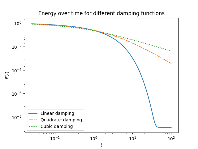
Figure 1: Damping rates, starting from random initial data. After a start-up period, the energy decays like $1/t$ for the cubic damping, $1/t^{2}$ for quadratic, and exponentially for the linear damping.

In Figure 2, we consider the case of two distinct random initial conditions, subjecting both the the forcing $(F,v)=\frac{\beta}{\epsilon^{2}}\sin(t)\left(xy,\nabla\cdot v\right)$ and measure the energy of the differences between solutions over time $[0,100]$. As with the damping, the eventual observed rates match those predicted theory, although there is a residual energy like in the damping example.

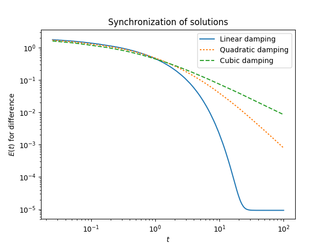
Figure 2: Synchronization rates, starting from random initial data. After a start-up period, the energy of the difference decays like $1/t$ for the cubic damping, $1/t^{2}$ for quadratic, and exponentially for the linear damping until a residual energy of $\mathcal{O}(\Delta t^{2})$ is reached.

5.2 Convergence

We used the method of manufactured solutions on the unit square, setting the problem coefficients to unit value and choosing forcing functions to make

$$\begin{split}u(x,y,t)&=\cos(\pi t)\begin{bmatrix}\sin(\pi x)\cos(\pi y),&\cos(\pi x)\sin(\pi y)\end{bmatrix}^{T}\\ \eta(x,y,t)&=\sin(\pi x)\sin(2\pi y)\cos(\pi t)\end{split}$$ (112)

In each case, we computed the solution until $T=10$, measuring the $L^{2}$ error of both $u$ and $\eta$ at each time step. We observed full first-order convergence, which is predicted in the linear case. In the nonlinear cases, it is not clear whether Theorem 111 is suboptimal, the calculation has not run on a long enough time horizon, or there is some other consideration. At any rate, we have confirmed similar second-order convergence when using the next-to-lowest order Raviart-Thomas element.

6 Conclusions

In this paper we introduced several results that underpin the application of compatible finite element spaces to barotropic tide modelling with nonlinear drag terms that are used in barotropic global tide models. By importing results from nonlinear PDEs, we were able to show that the numerical discretisation has a global attracting solution. Calculating this solution is the goal of barotropic tide modelling, since the Earth’s tides are assumed to have being occuring on a long enough time scale that memory of the initial conditions or past changes in topography are not relevant. The proof requires some assumptions of linear growth at infinity of the damping term, but in practice any reasonable damping model can be adjusted a posteriori to have linear growth at values that are never attained in the model solutions. We then provided two error analyses. The first is over finite time intervals, and predicts optimal scaling with mesh resolution, but with constant of proportionality growing exponentially in time. The second is global in time, but we obtain a suboptimal scaling with mesh resolution; numerical experiments confirm that our estimate is not sharp. However, our analysis does show that the numerical attracting solution converges to the true attracting solution as the mesh is refined, i. e. we have a convergent numerical solution to the barotropic tidal prediction problem.