Exact solution of anisotropic compact stars via. mass function

Abstract

The interest in studying relativistic compact objects play an important role in modern astrophysics with an aim to understand several astrophysical issues. It is therefore natural to ask for internal structure and physical properties of specific classes of compact star for astrophysical observable, and we obtain a class of new relativistic solutions with anisotropic distribution of matter for compact stars. More specifically, stellar models, described by the anisotropic fluid, establish a relation between metric potentials and generating a specific form of mass function are explicitly constructed within the framework of General Relativity. New solutions that can be used to model compact objects which adequately describe compact strange star candidates like SMC X-1, Her X-1 and 4U 1538-52, with observational data taken from Gangopadhyay et al. Gangopadhyay . As a possible astrophysical application the obtained solution could explain the physics of self-gravitating objects, might be useful for strong-field regimes where data are currently inadequate.

I.   Introduction

Over the past few years, there has been growing interest in static spherically symmetric compact object consistent with general relativity which are most often observed as pulsars, spinning stars with strong magnetic fields. However, in spite of the fact, it is important to know the exact composition and nature of particle interactions, which allow us to completely describe them in terms of their mass, spin angular momentum and charge. In particular, observations of compact stars are considered primary targets of the forthcoming field of gravitational wave astronomy. In the recent times we have experimental evidence that such objects do exist from observations with very high densities Lattimer , and some of the compact objects like X-ray pulsar Her X-1, X-ray burster 4U 1820-30, X-ray sources 4U 1728-34, PSR 0943+10, millisecond pulsar SAX J 1808.4-3658, and RX J185635-3754 strongly favour the possibility that they could actually be strange stars. In other words, there is no any strong evidence to make conclusion/ understood the mechanism about compact objects. In spite of this drawback, the internal composition and consequent geometry of such objects are still considered an open question in the scientific community. From a theoretical point of view, such compact objects are composed of a perfect fluid Ivanov . Generally, polytropic equation of state (EOS) in the form P = k $\rho^{\gamma}$ and bag model Witten ; Glendenning have widely used to describe a white dwarf or a less compact star Shapiro . An example, Herrera and Barreto Barreto carry out a general study on polytropic general relativistic stars with anisotropic pressure whereas Lai and Xu Lai have studied polytropic quark star model.

Though, interior of a star is an important astrophysical question and hence it is pertinent to construct relativistic models by assuming anisotropy fluid distribution. The theoretical study of the influence of anisotropic compact objects was first initiated by Bowers and Liang Bowers and another investigation led be Ruderman Ruderman showed that nuclear matter may have anisotropic features at least in certain very high density ranges $10^{15}$ g/$cm^{3}$, where the nuclear interaction must be treated relativistically. Later on, several models (see for example, Gleiser ; Dev2003 ; Herrera2002 ) have been proposed in this direction. The procedure has been found to be interesting and useful on the physical grounds that anisotropy affects the critical mass, mass-radius relation and stability of highly compact relativistic bodies. It is also well-established fact that a magnetic field acting on a Fermi gas produces pressure anisotropy was discussed recently in Chaichian ; Martinez ; Ferrer . Recently, Maurya and Gupta in Maurya2015a ; Maurya2016a have studied charged anisotropic stars whereas without charged solution has been analysed in Hossein ; Mehedi2012 . The role of anisotropy, with the linear equation of state was pursed by Mak and Harko Mak(2002) , and extending the work by Sharma and Maharaj Sharma obtained an exact analytical solutions assuming a particular form of mass function. In yet another paper, Victor Varela et al Varela studied Charged anisotropic matter with linear or nonlinear equation of state .

However, it has recently been proposed that an arbitrary d dimensional (pseudo-) Riemannian space can always be locally embedded into any Riemann space of dimension N $\geq$ d(d + 1)/2. Riemann’s seminal work in 1868 Riemann had inspired Schl$\ddot{a}$fli that how one can locally embed such manifolds in Euclidean space Schlafli . He discussed the local form of the embedding problem and conjectured that maximum number of extra dimensions that can embedded as a submanifold of a Euclidean space $E_{N}$ with N= $\frac{1}{2}n(n+1)$ or, equivalently, when the codimension r = N - n it gives r = n(n - 1)/2. Furthermore, one motivation in the treatment of embedding has been devoted, namely, Randall- Sundrum braneworld model is based on the assumption that four dimensional space-time is a three-brane, embedded in a five-dimensional Einstein space Randall . On the other hand Nash in 1956 nash established the idea of global isometric embedding theorem of $V_{n}$ into Euclidean space $E_{N}$.

In a sense one could say that all Riemannian manifold has a local and a global isometric embedding in an Euclidean space. This result opened new perspectives in embedding theorems with increasing degrees of generality and soon it became an powerful tool to construct and classify solutions of GR. Inspired by these advances, a popular approach has been emerged in embedding 4-dimensional space-time into 5-dimensional flat space-time by using the spherical coordinates transformation and known as embedding class one if it satisfies the Karmarkar condition Karmarkar . One of the primary motivations of such embedding is to establish a relationship between metric potentials and obtained exact solutions of Einstein’s equation to a single-generating function. In connection to this an exact anisotropic solution of embedding class one, has been developed in Maurya(2016) ; Maurya2017a ; Newton2016 . They showed that in seeking solution for relativistic static fluid spheres one can utilized this technique successfully. Motivated by the above facts, we will see how this theorem can be utilized for obtaining an exact solution of Einstein’s field equation for compact star models. In this article we consider the static spherically symmetric spacetime metric with embedding class one conditions, which can be altered to fit with a set of astrophysical objects.

This paper is outlined in the following manner. In Sec. II, we present the structural equations for anisotropic fluid distributions of stellar models applying the embedding class one conditions. Specific models are then analyzed in a brief description by obtaining a particular form of mass function. In Section III, we match our interior solution to an exterior Schwarzschild vacuum solution at the boundary surface and then determine the values of constant parameters. In Section IV, we continue our discussion thorough geometrical analysis of the solution such as energy conditions, hydrostatic equilibrium and stability of the star by fixing of certain parameters. We end our discussion by concluding remarks in V.

II.  Class one condition for Spherical symmetric metric and General relativistic equations

The simplest configuration for a star is the static and spherically symmetric geometry has the usual form

$$ds^{2}=e^{\nu(r)}dt^{2}-e^{\lambda(r)}dr^{2}-r^{2}\left(d\theta^{2}+\sin^{2}\theta d\phi^{2}\right),$$ (1)

where the coordinates (t, r, $\theta$, $\phi$) are the spherical coordinates and the metric coefficient $\lambda$ and $\nu$ are the functions of the radial coordinate $r$, and yet to be determined by solving the Einstein equations.

As the metric (1) is time independent and spherically symmetric, we restrict ourselves that the space time is of emending class one, if it satisfies the Karmarker condition (see Ref. Karmarkar ; Maurya(2016) for more details discussion) and metric functions $e^{\lambda}$ and $e^{\nu}$ are dependent on each other as:

$$e^{\lambda}=1+K\,F^{\prime 2},$$ (2)

where  $F=e^{\nu/2}$, $F=F(r)$ and $K>0$. However $F$ = constant, leads to flat space time metric.

The energy momentum tensor $T_{\mu\nu}$ associated to a spherical distribution of matter bounded by gravitation is locally anisotropic, that is $T_{\mu\nu}$ = $\text{diag}\left(\rho,-p_{r},-p_{t},-p_{t}\right)$, where $p_{r}$ and $p_{t}$ are the radial and tangential pressures and $\rho$ is the energy density of the fluid, respectively. Thus, the Einstein field equation, $G_{\mu\nu}$ = 8$\pi T_{\mu\nu}$, where $G_{\mu\nu}$ is the Einstein tensor then reduce to the following ordinary differential equations for the metric (since we use natural units where G = c = 1) as:

$$8\pi\,\rho(r)=e^{-\lambda}\,\left[\frac{\lambda^{\prime}}{r}+\frac{e^{\lambda}-1}{r^{2}}\right],$$ (3)

where the primes ($\prime$) denote differentiation with respect to r. Then one may write the solution in a very familiar form of mass function of the compact object,

$$m(r)=\int_{0}^{r}{4\,\pi\,r^{2}\,\rho(r)\,dr}.$$ (4)

It is worth noting that the mass is the density inside a proper volume element within a radius r. Using the above Eq. (4) and Eq. (2), we can write the metric component $e^{\lambda}$ which is given by the equality

$$e^{-\lambda}=1-\frac{2m}{r}=(1+K\,F^{\prime 2})^{-1}.$$ (5)

Rewriting the above expression in terms of mass function as:

$$m(r)=\frac{K\,r\,F^{\prime 2}}{2\,(1+K\,F^{\prime 2})}\,\,\,~{}~{}\text{or}~{}~{}\,\,F^{\prime 2}=\frac{2m}{K\,(r-2m)}.$$ (6)

Since $F^{\prime}(0)=0$ and $F^{\prime\prime}(0)>0$ because $F=e^{\nu/2}$, $\nu^{\prime}(0)=0$ and $\nu^{\prime\prime}(0)>0$ which is already proved by Herrera et al. Herrera1 and Maurya et al. Maurya1 . From Eq. (6), we obtain $m(0)\,=\,m^{\prime}(0)\,=\,m^{\prime\prime}(0)=0$ and $m^{\prime\prime\prime}(0)=3\,F^{\prime\prime}(0)/K>0$. This solution clearly implies that $m(r)$ is positive and monotonic increasing function of r.

It is possible to derive the mass function in terms of F(r). Aiming this the value of F(r) from Eq. (6), we have

$$F(r)=\frac{1}{\sqrt{K}}\,\int{\sqrt{\frac{2m}{r-2m}}}.$$ (7)

To solve this integral, we shall assume $2m(r)=r-f(r)$, that we claim $f(r)$ should be zero at centre i.e. $f(0)=0$ due to m$(0)=0$, which indicating that the mass function is regular at the origin. Equation (7) can be rewritten as

$$F(r)=\frac{1}{\sqrt{K}}\,\int{\sqrt{\frac{r-f(r)}{f(r)}}}.$$ (8)

To make the above integral equations tractable and construct a physically viable model, we suppose that $\frac{r-f(r)}{f(r)}=ar^{4}+br^{2}$ in a particular form, which gives

$$f(r)=\frac{r}{ar^{4}+br^{2}+1}.$$ (9)

where two constants a, b are positive and makes the Eq. (8) in a simplest form

$$F(r)=\frac{1}{\sqrt{K}}\,\int{\sqrt{a\,r^{4}+b\,r^{2}}}.$$ (10)

Solving the integral gives

$$F=A+\frac{(a\,r^{2}+b)^{3/2}}{3\,a\,\sqrt{K}},$$ (11)

where A stands for integrating constant. Substituting Eq. (11) in Eq. (2), we obtain one of the metric coefficient in the form

$$e^{\lambda}=1+b\,r^{2}+a\,r^{4},$$ (12)

and the mass function is given by

$$m(r)=\frac{r^{3}\,(a\,r^{2}+b)}{2\,\Bigl{(}1+b\,r^{2}+a\,r^{4}\Bigl{)}}.$$ (13)

The motivation of choice for particular dimensionless function lies on the fact that the obtained mass function a monotonic decreasing energy density in the interior of the star. To construct a physically viable model this type of mass function is not new but similar works have been considered earlier by Matese & Whitman Matese and Finch & Skea Finch for isotropic fluid spheres, and Mak & Harko Mak for anisotropic fluid spheres.

The system of equations used to study for spherically symmetric configurations with anisotropic fluid distribution are

$$8\pi\,\rho(r)=\frac{b^{2}\,r^{2}+a\,r^{2}\,(5+a\,r^{4})+b\Bigl{(}3+2\,a\,r^{4}\Bigl{)}}{\Bigl{(}1+b\,r^{2}+a\,r^{4}\Bigl{)}^{2}},$$ (14)

$$8\pi\,p_{r}(r)=-\frac{1}{\Bigl{(}a\,r^{4}+b\,r^{2}+1\Bigl{)}}\left[{b+a\,\left(r^{2}-\frac{6\,B\,\sqrt{a\,r^{2}+b}}{A+B\,(a\,r^{2}+b)^{3/2}}\right)}\right],$$ (15)

$$8\pi\,p_{t}(r)=\frac{a^{2}\,r^{2}\,B\,(a\,r^{4}+b\,r^{2}+9)-b\,(b^{2}\,B+A\,\sqrt{a\,r^{2}+b})+f_{1}(r)}{\sqrt{ar^{2}+b}~{}~{}\Bigl{(}1+br^{2}+ar^{4}\Bigl{)}^{2}~{}~{}\Bigl{[}A+B(b+ar^{2})^{3/2}\Bigl{]}},$$ (16)

where we use $f_{1}(r)=a\,\left[6\,b\,B-b^{2}\,B\,r^{2}-2\,A\,r^{2}\,\sqrt{ar^{2}+b}\right]$ for our notational convention.

Firstly, we will present the anisotropic effect by a term $(p_{t}-p_{r})/r$, by taking into account Eqs. (15-16), may be expressed in the following equivalent form

$$\Delta=\frac{r^{2}\,\Bigl{[}B\,(b^{2}+a^{2}\,r^{4})+A\,g-a\,B\,(3-2\,b\,r^{2})\,(b^{2}+a^{2}\,r^{4}-a+2\,a\,b\,r^{2})\,\Bigl{]}}{8\pi\,\sqrt{a\,r^{2}+b}~{}~{}\Bigl{(}1+b\,r^{2}+a\,r^{4}\Bigl{)}^{2}~{}~{}\Bigl{[}A+B(b+ar^{2})^{3/2}\Bigl{]}},$$ (17)

which representing a force that is due to the anisotropic nature of the fluid. The anisotropy will be repulsive or directed outwards if $p_{t}>p_{r}$, and attractive or directed inward when $p_{t}<p_{r}$. The effects of anisotropy forces maintain the stability and equilibrium configurations of a stellar stricture, as we discuss later.

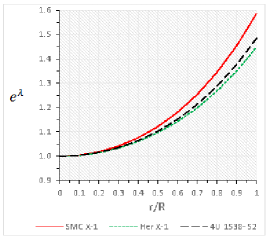
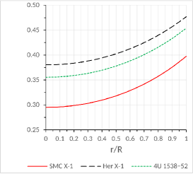
Figure 1: Variation of the metric coefficient $e^{\lambda}$ and $e^{\nu}$ are shown as a function of radial coordinate for compact stars candidates SMC X-1, Her X-1 and 4U 1538-52 with their respective parameters given in Table 1. Note that, qualitatively, the nature of $e^{\lambda}$ and $e^{\nu}$ are monotonic increasing towards the boundary.

In more detail, it is important to emphasize the results. That’s why we extend our calculation for the first order differential equation, which are

$$\frac{d\rho}{dr}=-\frac{2\,r\,\left[\,a^{3}r^{8}+3a^{2}r^{4}(4+br^{2})+b^{2}(5+br^{2})+a(-5+13br^{2}+3b^{2}r^{4})\,\right]}{8\pi\,\Bigl{(}1+br^{2}+ar^{4}\Bigl{)}^{3}},$$ (18)

$$\frac{dp_{r}}{dr}={\frac{-2ar\,(g\,f^{2}+9\,a\,B^{2}g^{3}-3\,a\,B\,f)}{8\,\pi\,g~{}f^{2}\,\Bigl{(}1+b\,r^{2}+a\,r^{4}\Bigl{)}}}+\frac{2\,r\,(2\,a\,r^{2}+b)\,(f~{}g^{2}-6\,B\,g)}{8\,\pi\,\Bigl{(}1+b\,r^{2}+a\,r^{4}\Bigl{)}^{2}~{}f},$$ (19)

$$\frac{dp_{t}}{dr}=\frac{2\,r\,\Bigl{[}\,\Psi_{1}(r)+\Psi_{2}(r)+\Psi_{3}(r)+\Psi_{4}(r)+\Psi_{5}(r)\,\Bigl{]}}{16\,\pi\,\,(b+ar^{2})^{3/2}(1+br^{2}+ar^{4})^{3}\Bigl{[}A+B(b+ar^{2})^{(}3/2)\Bigl{]}^{2}},$$ (20)

for our notational conventional we use $f=\Bigl{[}A+B(b+ar^{2})^{3/2}\Bigl{]}$,    $g=\sqrt{b+ar^{2}}$,     and

$\Psi_{1}(r)=-6a^{6}B^{2}r^{12}g+4b^{3}\Bigl{[}2Ab^{2}B+A^{2}g+b^{3}B^{2}g]+a^{5}Br^{8}[15Ar^{2}-2Bg(44+9br^{2})\Bigl{]}$,

$\Psi_{2}(r)=2ab\Bigl{[}-11b^{3}B^{2}gh-2A^{2}g(4h-3)-Ab^{2}B(21h-8)\Bigl{]}$,

$\Psi_{3}(r)=-a^{4}Br^{4}\,\Bigl{[}-7Ax(-8+9br^{2})+2Bg(9+131br^{2}+4b^{2}r^{4})\Bigl{]}$,

$\Psi_{4}(r)=a^{2}\Bigl{[}4A^{2}r^{2}g(-1+6br^{2})-2b^{2}B^{2}g(3+65br^{2}-21b^{2}r^{4})+3AbB(4-31br^{2}f)\Bigl{]}$,

$\Psi_{5}(r)=a^{3}r^{2}\Bigl{[}12A^{2}r^{4}g-2bB^{2}g[12+br^{2}(141-14br^{2})]+AB(9-123br^{2}+107b^{2}r^{4})\Bigl{]}$.

We exercised our results in various ways first by checking calculation and putting restriction on the physical parameter based on logarithmic principle and then by using graphical representation which are illustrated in Figs. (1-3), describing the metric functions, energy density, radial and transverse pressures and measure of anisotropic within the given radius. In the next section we will look for supplementary restrictions on the model to make it physically viable.

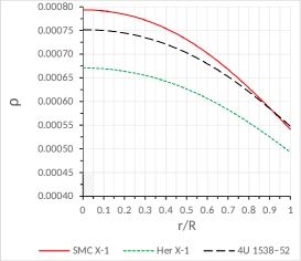
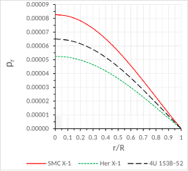
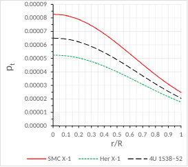
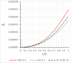
Figure 2: The energy density, radial pressure, transverse pressure and anisotropy factor in their normalized forms as a function of the radial coordinate are shown according to Eq. (14-17). The pressure anisotropy is positive in the interior of star, i.e., force due to the anisotropic nature is directed outward.

III.   Boundary conditions

To do the matching properly, we start by joining an interior spacetime $\mathcal{M_{-}}$, to an exterior $\mathcal{M_{+}}$, Schwarzschild vacuum solution at the boundary surface r = R. At this boundary the metric should be continuous. The Schwarzschild solution is given by

$$\qquad\qquad ds^{2}=\left(1-\frac{2M}{r}\right)\,dt^{2}-\left(1-\frac{2M}{r}\right)^{-1}dr^{2}-r^{2}(d\theta^{2}+\sin^{2}\theta\,d\phi^{2}),$$

where $M$ denote the total mass of the compact star. In deciding criterions for an anisotropic compact star the radial pressure $p_{r}$ must be finite and positive inside the stars, and it should vanishs at the boundary $r=R$ of the star Misner .

In determining the value of constrains parameters we use the boundary condition $p_{r}(R)=0$, which can express as

$$\frac{A}{B}=\frac{\sqrt{b+a\,R^{2}}~{}\Bigl{[}\,6aB-b^{2}B-2\,a\,b\,B\,R^{2}-a^{2}\,B\,R^{4}\,\Bigl{]}}{(b+a\,R^{2})}.$$ (22)

In order to match smoothly on the boundary surface, we must require the continuity of the first and the second fundamental forms across that surface. Then it follows the condition $e^{\nu(R)}=e^{-\lambda(R)}$ which gives the value of constant parameter B as

$$B=\frac{1}{\sqrt{1+bR^{2}+aR^{4}}~{}\left[\,\frac{A}{B}+(aR^{2}+b)^{3/2}\,\right]},$$ (23)

and using the condition $e^{-\lambda(R)}=1-\frac{2M}{R}$, we have

$$M=\frac{R^{3}\,\left(aR^{2}+b\right)}{1+bR^{2}+aR^{4}}.$$ (24)

This represents the total mass of the sphere as seen by an outside observer. Additionally, bounds on stellar structures is an important source of information and classification criterion for compact objects, to determine the mass-radius ratio which was proposed by Buchdahl Buchdahl . This bound has been considered for thermodynamically stable perfect fluid compact star with ratio 2M/R, must be less than 8/9. We have carried out the analysis for our compact star candidates SMC X-1, Her X-1 and 4U 1538-52, that are used to calculate the values of constants A and B. For this purpose, we present these results (central density, surface density, central pressure, mass-radius ratio) in table I & II, respectively.

Table I	Numerical values of the parameters or constants for different compact stars  Gangopadhyay
Compact Star	R (km)	M$\left(M_{\odot}\right)$	$~{}~{}~{}a\,(km^{-4})$	$b\,(km^{-2})$	A	$B(km^{3})$
SMC X-1	8.301	1.04	0.0000270	0.006648	0.439167064	452.08447
Her X-1	8.1	0.85	0.0000185	0.005620	0.481332147	618.82624
4U 1538-52	7.866	0.87	0.0000247	0.006300	0.481382726	490.02078

Let us now focus on surface gravitational redshift, which gives a wealth of information about compact objects, and defined by Z = $\Delta\lambda/\lambda_{e}$ = $\frac{\lambda_{0}-\lambda_{e}}{\lambda_{e}}$, where $\lambda_{e}$ is the emitted wavelength at the surface of a nonrotating star and the observed wavelength $\lambda_{e}$. Thus one can estimate the gravitational redshift, defined by $Z_{s}$, from the surface of the star as measured by a distant observer by the following relation

$$Z_{s}=-1+\Bigl{\rvert}g_{tt}(R)\Bigl{\rvert}^{-1/2}=-1+\left(1-\frac{2M}{R}\right)^{-1/2},$$ (25)

where $g_{tt}$ = $e^{\nu(R)}$ = $\left(1-\frac{2M}{R}\right)$. Measurement of the gravitational redshift for a static perfect fluid sphere is not larger than $Z_{s}$ = 2 Buchdahl , whereas for an anisotropic fluid sphere this value may be increase up to $Z_{s}$ = 3.84, as given in Ref. Ivanov . We are trying to estimate the surface redshift given table II for different compact star candidates.

Table II	Estimated physical values based on the observational data and theory
Compact star	$\rho_{0}(gm/cm^{3})$	$\rho_{R}(gm/cm^{3})$	$p_{c}(dyne/cm^{2})$	$2M/R$	$~{}~{}~{}Z_{s}$
SMC X-1	1.0710$\times 10^{15}$	7.3060$\times 10^{14}$	1.0052$\times 10^{35}$	0.36959 $<$ 8/9	0.25948
Her X-1	9.0538$\times 10^{14}$	6.6539$\times 10^{14}$	6.3783$\times 10^{34}$	0.30957 $<$ 8/9	0.20348
4U 1538-52	1.0149$\times 10^{15}$	7.3928$\times 10^{14}$	7.9036$\times 10^{34}$	0.32628 $<$ 8/9	0.218346

IV.   Physical features and Comparative study of the physical parameters for compact star model

To proceed further discussion based on the obtained solution that must satisfy some general physical requirements. In order to simplify the analysis and make the solution more viable we explore some physical features of the compact star and carry out a comparative study between the data of the model parameters with a set of astrophysical objects in connection to direct comparison of some strange/compact star candidates.

.1 Energy Conditions

Let us first discuss a very simple but important features of a stellar model. The study of energy conditions within the framework of GR is an essential part for studying the compact objects. Here we examine the energy conditions, namely : (i) Null energy condition (NEC), (ii) Weak energy condition (WEC) and (iii) Strong energy condition (SEC), at all points in an interior of a star holds simultaneously, by the following inequalities

$$\textbf{NEC:}~{}\rho(r)-p_{r}\geq 0,$$ (26)

$$\textbf{WEC:}~{}\rho(r)-p_{r}(r)\geq 0~{}~{}(WEC_{r}),~{}~{}~{}\rho(r)-p_{t}(r)\geq 0~{}~{}(WEC_{t}),$$ (27)

$$\textbf{SEC:}~{}\rho(r)-3p_{r}(r)\geq 0~{}~{}(SEC_{1}),~{}~{}~{}\rho-p_{r}(r)-3p_{t}(r)\geq 0~{}~{}(SEC_{2}).$$ (28)

From the above inequalities we provide a graphical representation that one can easily justify the nature of energy condition for three different compact objects in Fig. 3. Due to the complexity of the expression, we only able to write down the above inequalities and plotted the graphs against the above criterions. In fact, all the energy conditions are not violated and well behaved in the stellar interior.

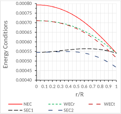
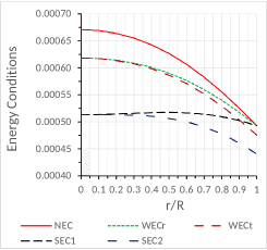
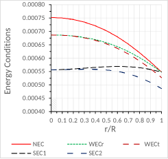
Figure 3: The standard energy conditions of GR have been plotted, namely, NEC, WEC and SEC with the radial coordinate inside stellar structure for different compact star candidates SMC X-1, Her X-1 and 4U 1538-52 from left to right. In every cases it satisfies all energy conditions and the parameter values have been taken for the graphs from Table 1.

.2 Generalized Tolman-Oppenheimer-Volkov Equation

On the other hand, for a given compact star, it is possible to test for hydrostatic equilibrium under the different forces namely gravitational, hydrostatic and anisotropic forces. Nevertheless, in our investigations we need to apply generalized Tolman-Oppenheimer-Volkov (TOV) equation Oppenheimer1939 ; Leon1993 , which is commonly used for an anisotropic fluid distribution is given by

$$\qquad-\frac{M_{G}(r)(\rho+p_{r})}{r^{2}}e^{\frac{\lambda-\nu}{2}}-\frac{dp_{r}}{dr}+\frac{2}{r}(p_{t}-p_{r})=0,$$ (29)

where the effective gravitational mass $M_{G}(r)$ is defined by

$$\qquad\hskip 28.45274ptM_{G}(r)=\frac{1}{2}{{r}^{2}}e^{\frac{\nu-\lambda}{2}}\nu^{\prime}.$$ (30)

Then equation (29) may be rewritten as

$$\qquad-\frac{\nu^{\prime}}{2}(\rho+p_{r})-\frac{dp_{r}}{dr}+\frac{2}{r}(p_{t}-p_{r})=0,$$ (31)

Let us now attempt to explain the Eq. (31) from an equilibrium point of view, which was first shown by Tolman Tolman1939 and Oppenheimer and then Volkoff Oppenheimer1939 , where they predicted the stable equilibrium condition for the compact star as a sum of three different forces, viz. gravitational force ($F_{g}$), hydrostatics force ($F_{h}$) and anisotropic force ($F_{a}$). Thus the above condition assumed the following form, namely

$$F_{g}+F_{h}+F_{a}=0.$$ (32)

The components of forces can be expressed in explicit form as:

$$\quad F_{g}=\frac{-\nu^{\prime}(\rho+p_{r})}{2}=-\frac{6ar\,B\,g}{8\,\pi}\,\left[\frac{A\,(b+2ar^{2})+B\,g~{}[b^{2}+5a^{2}r^{4}+a\,(3+6br^{2})]}{(1+br^{2}+ar^{4})^{2}\,[A+B\,(b+ar^{2})^{3/2}]^{2}}\right],$$ (33)

$$\quad F_{h}=-\frac{dp_{r}}{dr}=\frac{a\,r}{(1+b\,r^{2}+a\,r^{4})}{\,\left[\frac{gf^{2}+9\,aB^{2}g^{3}-3\,a\,B\,f}{4\,\pi\,g~{}~{}f^{2}}\right]}-\frac{r\,(2\,a\,r^{2}+b)}{(1+b\,r^{2}+a\,r^{4})^{2}}\left[\frac{g^{2}\,f-6\,B\,g}{4\,\pi\,f}\right],$$ (34)

$$\quad F_{a}=\frac{2}{r}(p_{t}-p_{r})=\frac{r\,[B\,(b^{2}+a^{2}\,r^{4})+A\,\sqrt{a\,r^{2}+b}-a\,B\,(3-2\,b\,r^{2})\,(b^{2}+a^{2}\,r^{4}-a+2a\,b\,r^{2})\,]}{4\,\pi\,\sqrt{ar^{2}+b}~{}~{}\left(1+br^{2}+ar^{4}\right)^{2}~{}~{}\left[A+B(b+ar^{2})^{3/2}\right]},$$ (35)

At this point in the derivation, a stable configuration of the system is counter balance by the components of different forces. To illustrate this in more detail let us introduce an graphical representation as evidenced in Fig. 4.

Here, the combine forces of hydrostatic ($F_{h}$) and anisotropic ($F_{a}$), dominate the gravitational force ($F_{g}$), while the anisotropic stress has a less role to the action of equilibrium condition. Hence, following the reason outlined above and making use of Eq. (32), we established the stable configuration model as shown in Fig. 4.

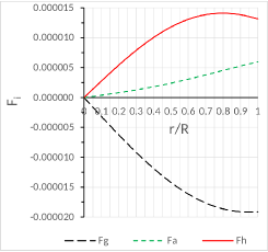
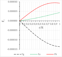
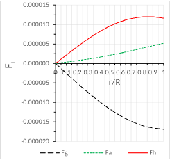
Figure 4: Plots for the variation of different forces, namely, gravitational force ($F_{g}$), hydrostatics force ($F_{h}$) and anisotropic force ($F_{a}$) with the radial coordinate inside stellar structure. For compact star candidates SMC X-1, Her X-1 and 4U 1538-52, different forces have been plotted from left to right. See the text for details about how they maintain the stable configuration mode.

.3 Stability Analysis

In this section we analyze the speed of sound propagation $v^{2}_{s}$, is given by the relation $v^{2}_{s}=dp/d\rho$. For a physically interesting stellar geometry should require that the sound speed does not exceed the speed of light, i.e., the physically relevant region is always less than unity. Here we will investigate the speed of sound for anisotropic fluid distribution and propagating along radial as well as transverse direction, should satisfy the bounds $0<v_{r}^{2}=\frac{dp_{r}}{d\rho}<1$ and $0<v_{t}^{2}=\frac{dp_{t}}{d\rho}<1$, Herrera(2016) .

We first carry out an analysis of sound velocity with graphical representation. Our result for obtained velocity of sound for compact star with anisotropic matter is presented in Fig. 5, for strange star candidates SMC X-1, Her X-1 and 4U 1538-52. As the resulting expressions are very elaborated, so we only plot the results for different compact stars. It is interesting to note that both $v_{r}^{2},\,v_{t}^{2}<1$ and monotonic decreasing function, which all show a behavior similar to that found for other compact objects. This is a sufficient condition for the solution to be causal. A notable characteristic of the sound velocity is the estimation of the potentially stable and unstable eras, by considering the expression $0<\Bigl{\rvert}v_{t}^{2}-v_{r}^{2}\Bigl{\rvert}\leq 1$, for stable potential Andreasson . According to Fig. 5 (extreme right) our solution gives us the stable star configuration.

Our investigation shows that obtained mass function by using the Karmarker condition for strange compact star matter, satisfies both energy and stability conditions

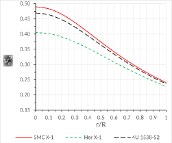
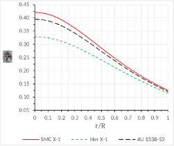
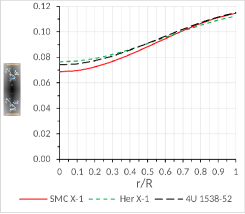
Figure 5: Illustrative plots for speed of sound propagation $v_{s}^{2}=dp/d\rho$ along the radial and transverse direction for the same stars. For a view on the status it’s clearly that the speed of sound is less than unity. In extreme right position we have drawn the graphs for $\Bigl{\rvert}v_{t}^{2}-v_{r}^{2}\Bigl{\rvert}$ using the same parameters enlisted in table 1.

I Concluding Remarks

To summarize, we have studied compact objects supported by anisotropic fluid distribution, which plays an important role in preventing gravitationally collapse. The motivation behind such a construction is that, we established a relation between metric potentials by imposing an embedding theorem, known as embedding class one within the framework of GR. As a result of this approach, we generate a mass function which we have used to study the interior of stellar objects with density decreasing outwards. In next, we have started by deriving the basic equations of Einstein’s field equations that describing the structure of compact objects.

In section (II), using the structural equations we derived the energy density, radial and transverse pressures and measure the nature of anisotropy. The complicated expressions given by equations (14-17) are plotted as a function of the radius for our compact stars candidates SMC X-1, Her X-1 and 4U 1538-52. An important feature of this model is the energy density might not vanish at the boundary r =R, though the radial pressure vanishes for all parameter values in according to the boundary condition. Additionally, at the boundary the interior spacetime have been matched by a Schwarzschild metric, and determine the values of arbitrary constants A and B for our compact stars candidates SMC X-1, Her X-1 and 4U 1538-52 in section (III). A comparative study of our results with that of the compact star candidates are provided in Table I and II.

Once the mass function is specified, in order to close the system based on physical requirements, we further proceed by investigating the energy conditions, hydrostatic equilibrium under the different forces, and velocity of sound. All the physical properties are well behaved within the stellar radius. We also showed that upper bound of the mass-radius ratio must be less than 8/9 as proposed by Buchdahl Buchdahl , for different compact star candidates which we have used for our model.

This indicates that the approach adapted in this paper is likely to produce other meaningful models with specific mass function that also greatly help in understanding the properties of other different static compact configurations. In our further study it would be interesting to investigate other forms of mass function that exhibit more general behaviour and thereby describe strange stars related with observational details.

References

- (1) T. Gangopadhyay et al.: Mon. Not. R. Astron. Soc., 431, 3216 (2013).
- (2) J. Lattimer: (2010) http://stellarcollapse.org/nsmasses.
- (3) B. V. Ivanov: Phys. Rev. D, 65, 104011 (2002).
- (4) E. Witten: Phys. Rev. D, 30, 272 (1984).
- (5) N. K. Glendenning, Ch. Kettner & F. Weber: Phys. Rev. Lett., 74, 3519 (1995).
- (6) S. L. Shapiro & S. A. Teukolosky: Black Holes, White Dwarfs and Neutron Stars: The Physics of Compact Objects (Wiley, New York,1983).
- (7) L. Herrera & W. Barreto: Phys. Rev. D., 88, 084022 (2013).
- (8) X.Y. Lai & R.X. Xu: Astropart.Phys., 31, 128-134 (2009).
- (9) R.L. Bowers & E. P. T. Liang: Class. Astrophys. J., 188, 657 (1974).
- (10) R. Ruderman: Rev. Astr. Astrophys., 10, 427 (1972).
- (11) K. Dev & M. Gleiser: Gen. Rel. Grav., 34, 1793, (2002).
- (12) K. Dev & M. Gleiser: Gen. Rel. Grav., 35, 1435, (2003).
- (13) L. Herrera, J. Martin & J. Ospino: J. Math. Phys., 43, 4889, (2002).
- (14) M. Chaichian et al.: Phys. Rev. Lett, 84, 5261 (2000).
- (15) A. Perez Martinez, H. Perez Rojas & H. J. Mosquera Cuesta: Eur. Phys. J. C, 29, 111 (2003).
- (16) E. J. Ferrer et al.: Phys. Rev. C, 82, 065802 (2010).
- (17) S.K. Maurya et al.: Eur. Phys. J. C, 75, 389 (2015).
- (18) S.K. Maurya et al.: Astrophys. Space Sci., 361, 163 (2016).
- (19) Sk. Monowar Hossein et al.: Int.J.Mod.Phys. D, 21, 1250088 (2012).
- (20) Mehedi Kalam et al.: Eur. Phys. J. C, 72, 2248 (2012).
- (21) M.K. Mak & T. Harko: Chin. J. Astron. Astrophys.,, 2, 248, (2002).
- (22) R. Sharma & S. D. Maharaj: Mon. Not. R. Astron. Soc., 375, 1265 (2007).
- (23) Victor Varela et al.: Phys.Rev. D, 82, 044052 (2010).
- (24) B. Riemann & Abh. Knigl: gesellsch., 13, 1 (1868).
- (25) L. Schl: Ann. di Mat. srie 5, 170 (1871).
- (26) L. Randall & R. Sundrum: Phys. Rev. Lett., 83, 3370 (1999); : Phys. Rev. Lett., 83, 4690 (1999).
- (27) J. Nash: Ann. Math., 63, 20 (1956).
- (28) K. R. Karmarkar: Proc. Ind. Acad. Sci. A, 27, 56 (1948).
- (29) S. K. Maurya et al.: Eur. Phys. J. A, 52, 191 (2016).
- (30) S. K. Maurya et al.: Eur. Phys. J. C, 77, 45 (2017).
- (31) Ksh. Newton Singh et al.: Int.J.Mod.Phys. D, 25, 1650099 (2016).
- (32) L. Herrera : Phys. Lett. A, 165, 206 (1992).
-
(33)
H. A. Buchdahl: Phys. Rev., 116, 1027 (1959);
H. A. Buchdahl: Astrophys. J., 146 275, (1966). - (34) B. V. Ivanov: Phys. Rev. D, 65, 104011 (2002).
- (35) J. J. Matese & P. G. Whitman: Phy. Rev. D, 11, 1270 (1980).
- (36) M. R. Finch & J. E. F. Skea: Class. Quantum Grav., 6, 467 (1989).
- (37) M. K. Mak & T. Harko: Proc. Roy. Soc. Lond., A, 459, 393 (2003).
- (38) L. Herrera, J. Ospino & A. Di Parisco: Phys. Rev. D, 77, 027502 (2008).
- (39) S. K. Maurya, Y.K. Gupta & S. Ray: arXiv: 1502.01915 [gr-qc] (2015).
- (40) C. W. Misner & D. H. Sharp: Phys. Rev. B, 136, 571 (1964).
- (41) R.C. Tolman: Phys. Rev., 55, 364 (1939).
- (42) J.R. Oppenheimer & G.M. Volkoff: Phys. Rev., 55, 374 (1939).
- (43) J. Ponce de León: Gen. Relativ. Gravit., 25, 1123 (1993).
- (44) V. Varela: Phys. Rev. D, 82, 044052 (2010).
- (45) J. Devitt & P.S. Florides: Gen. Relativ. Gravit., 21, 585 (1989).
- (46) H. Andreasson: Commun. Math. Phys., 288, 715 (2009).