Conductance distribution in the magnetic field

1. Introduction

It is well-known that conductance of a disordered system is a strongly fluctuating quantity: its root-mean-square deviation in the metallic phase does not depend on the system size [1, 2] and becomes comparable with its mean in the vicinity of the Anderson transition; as a result the problem of its distribution $W(g)$ arises. Here and below $g=hG/e^{2}$ is a dimensionless conductance, which is determined by conductance $G$ of a sample in quantum units $e^{2}/h$.

In the recent paper [3], using a modification of the Shapiro approach [4, 5], we have introduced the two-parameter family of conductance distributions $W(g)$, which is in one-to-one correspondence with conductance distributions of quasi-1D systems of size $L^{d-1}\times L_{z}$ ($d$ is a dimension of space), characterizing by parameters $L/\xi$ and $L_{z}/L$ ($\xi$ is the correlation length). Investigation of this family allowed to describe all essential features of the distribution $W(g)$, established in numerical experiments, and reproduce the results for its cumulants derived in the sigma-model formalism [6]. The approach of [3] is based on the evolution equation for the distribution $P(\rho)$ of dimensionless Landauer resistances [7] ($\rho=1/g$) for one-dimensional systems, which are arranged by a certain scheme to compose the $d$-dimensional system [4, 5]. At first glance, generalization of these results [3] for the case of a non-zero magnetic field presents no problem: one should only use the 1D evolution equation without assumption of time-reversal invariance. However, realization of this scheme (Sec.2) meets two difficulties: (a) disagreement in the number of essential parameters, and (b) incorrect estimation of the critical behavior in $2+\epsilon$ dimensions. Analysis of these contradictions leads to conclusion (Sec.3) that they are related with a qualitative difference between quasi-1D and strictly one-dimensional systems in presence of the magnetic field. Replacement of the 1D evolution equation by the generalized Dorokhov–Mello–Pereyra–Kumar (DMPK) equation [8] eliminates the indicated problems (Sec.4). The evolution equation for $P(\rho)$ derived from the generalized DMPK equation (Sec.5) has the same structure as in the 1D case but with variable coefficients. The latter explains the origin of indicated difficulties, but becomes inessential after transition to the $d$-dimensional case (Sec.6). As a result, the conductance distribution in the magnetic field is described by the same equations as in the absence of a field; however, one of irrelevant parameters becomes relevant. Therefore, variation of the magnetic field does not lead to any qualitative effects in the conductance distribution and only changes its quantitative characteristics, moving a position of the system in the three-parameter space. These conclusions are in accordance with numerical experiments [9, 10].

2. The simplest scheme

The approach used in the paper [3] is based on the large-scale constructions by Shapiro [4, 5], analogous to the Migdal–Kadanov transformation in the usual phase transitions theory [11, 12]. Firstly, $b$ cubical blocks of size $L$ are arranged successively to form a quasi-one-dimensional system (Fig.1), and then a parallel connection of $b^{d-1}$ quasi-1D chains composes the $d$-dimensional cube of size $bL$. For simplicity, the quasi-1D systems are supposed to be isolated by dielectric inter-layers (Fig.1); however, in the large $L$ limit the concentration of the auxiliary dielectric phase tends to zero, and the Shapiro scheme looks well-grounded. Only the latter limit will be of interest for us (see a detailed discussion in [3]).

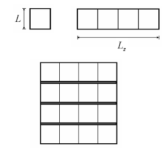
Figure 1: Large-scale constructions used in the Shapiro scheme: the cubical blocks of size $L$ are arranged into quasi-1D systems of length $L_{z}$, whose parallel connection composes the $d$-dimensional cube of the larger size.

According to the one-parameter scaling hypothesis [13], all properties of the cubic system of size $L$ are completely determined by the ratio $L/\xi$. The properties of the quasi-1D system, composed of cubical blocks, are specified by the properties of the single block ($L/\xi$) and a number of cubes ($L_{z}/L$), so for conductance

$$g=F\left(\,\frac{L}{\xi}\,,\,\frac{L_{z}}{L}\,\right)\,.$$

Setting $L=a$ ($a$ is the atomic spacing), one comes to conclusion, that the conductance distribution $W(g)$ of the quasi-1D system corresponds to a certain conductance distribution of the strictly one-dimensional system . This conclusion agrees with the fact that the well-known evolution equation for 1D systems [4, 14, 15, 16, 17]

$$\frac{\partial P(\rho)}{\partial L}=\alpha\frac{\partial}{\partial\rho}\left[\,\rho(\rho+1)\frac{\partial P(\rho)}{\partial\rho}\,\right]$$

allows two-parameter generalization

$$\frac{\partial P(\rho)}{\partial L}=\tilde{\alpha}\,\frac{\partial}{\partial\rho}\left[\,-\gamma(2\rho+1)P(\rho)+\rho(\rho+1)\frac{\partial}{\partial\rho}P(\rho)\,\right]\,,$$

so parameters $L/\xi$ and $L_{z}/L$ of equation (1) are in one-to-one correspondence with parameters $\tilde{\alpha}L$ and $\gamma$ specifying the solution of (3). We do not try to establish a character of this correspondence for any specific situations but investigate all family of distributions in whole. The properties of a quasi-1D system are described by equation (3) and can be considered as known in principle, so transition to the $d$-dimensional case presents no problem: it is sufficient to come from $P(\rho)$ to $W(g)$ and find the distribution of a sum of $b^{d-1}$ independent random quantities with the same distribution $W(g)$. This procedure can be realized in the differential form [3, 4, 5] and leads to the evolution equation describing the $d$-dimensional system (Sec.6).

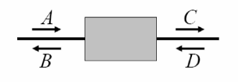
Figure 2: In one-dimensional systems, the transfer matrix $\hat{T}$ relates amplitudes of plane waves on the left and on the right of a scatterer.

In description of one-dimensional systems, it is convenient to consider each scatterer as ”a black box”, characterizing by a transfer matrix $\hat{T}$, relating amplitudes of the plane waves on the left ($Ae^{ikx}+Be^{-ikx}$) and on the right ($Ce^{ikx}+De^{-ikx}$) of the scatterer (Fig.2):

$$\left(\begin{array}[]{cc}A\\ B\end{array}\right)\,=\hat{T}\left(\begin{array}[]{cc}C\\ D\end{array}\right)\,.$$

A successive arrangement of scatterers corresponds to multiplication of transfer matrices. In the presence of time-reversal invariance, the transfer matrix allows a parametrization [18]

$$\hat{T}=\left(\begin{array}[]{cc}\sqrt{\rho\!+\!1}\,e^{-i\varphi}&-\sqrt{\rho}\,e^{-i\theta}\\ -\sqrt{\rho}\,e^{i\theta}&\sqrt{\rho\!+\!1}\,e^{i\varphi}\end{array}\right)\,,$$

so one should consider the mutual distribution function $P\left(\rho,\varphi,\theta\right)$ for the parameters entering (5). In the product of $n$ transfer matrices the distribution of phases $\varphi$ and $\theta$ is usually stabilized for large $n$, so

$$P_{n}\left(\rho,\varphi,\theta\right)=P_{n}\left(\rho\right)P\left(\varphi,\theta\right)\,.$$

If distribution of phases is uniform ($P\left(\varphi,\theta\right)=const$), then equation (2) is valid, while in the general case one obtains Eq.3 with parameters

$$\gamma=\frac{1-2A_{0}}{2A_{0}},\quad\tilde{\alpha}=2\alpha A_{0},\quad A_{0}=\left\langle\sin^{2}(\varphi-\theta)\right\rangle.$$

From the above discussion one can see a simple way to generalize the described procedure to the case of the non-zero magnetic field. It is sufficient to replace the transfer matrix (4) by the more general expression

$$\hat{T}=\left(\begin{array}[]{cc}\sqrt{\rho\!+\!1}\,e^{-i\varphi}&-\sqrt{\rho}\,e^{-i\theta+i\zeta}\\ -\sqrt{\rho}\,e^{i\theta}&\sqrt{\rho\!+\!1}\,e^{i\varphi+i\zeta}\end{array}\right)\,,$$

which is valid without assumption of the time-reversal invariance, and repeat derivation of the evolution equation (see Appendix 1); as a result, we come to the same equation (3) with parameters

$$\gamma=\frac{1-2A_{0}}{2A_{0}},\quad\tilde{\alpha}=2\alpha A_{0}\,,\quad A_{0}=\left\langle\sin^{2}(\varphi-\theta+\zeta)\right\rangle.$$

One can see that a presence of the magnetic field leads to the only effect that the phase $\zeta$, being strictly equal to zero in the absence of a field, acquires a certain stationary distribution; this changes coefficients of Eq.3 but does not change its structure. Using results of [3], we come to conclusion that the conductance distribution in the $d$-dimensional case is described by the same equations, as in the absence of a field.

However, on a closer examination the described scheme meets two difficulties. Firstly, in the presence of the magnetic field, Eq.1 is replaced by

$$g=F_{H}\left(\,\frac{L}{\xi}\,,\,\frac{L_{z}}{L}\,,\,\frac{L}{l_{H}}\,\right)\,,$$

where $l_{H}=(c\hbar/2eH)^{1/2}$ is the magnetic length. Setting $L=a$, we see that in description of one-dimensional systems one should have three essential parameters, and not two, as in Eq.3.

Secondly, there is a problem with estimation of the critical behavior of the correlation length $\xi$, given in Sec.5.1 of [3] and initially suggested by Shapiro [5]. Multiplying Eq.2 by $\rho$ and integrating, one has a closed equation for the average value $\left\langle\rho\right\rangle$, whose solution

$$\left\langle\rho_{L}\right\rangle={\textstyle\frac{1}{2}}\left(e^{2\alpha L}-1\right)$$

can be rewritten in the form of the scale transformation for 1D systems

$$\left\langle\rho_{bL}\right\rangle={\textstyle\frac{1}{2}}\left[\left(1+2\left\langle\rho_{L}\right\rangle\right)^{b}-1\right]\,.$$

For the parallel connection of $b^{d-1}$ one-dimensional chains, resistance is diminished by a factor $b^{d-1}$, and one has a scale transformation for the $d$-dimensional system:

$$\left\langle\rho_{bL}\right\rangle={\textstyle\frac{1}{2}}b^{-(d-1)}\left[\left(1+2\left\langle\rho_{L}\right\rangle\right)^{b}-1\right]\,.$$

If Eq.3 is used instead of (2), then dependence on $\gamma$ disappears and results (11–13) remain unchanged. In fact, for the parallel connection of chains the average conductances should be added, i.e. $\left\langle g_{bL}\right\rangle=b^{d-1}\left\langle g_{L}\right\rangle$ instead of the previously used relation $\left\langle\rho_{bL}\right\rangle=b^{-(d-1)}\left\langle\rho_{L}\right\rangle$. As a result, the scale transformation (13) is valid only for $d=2+\epsilon$, when the distribution $P(\rho)$ is narrow and two indicated relations approximately coincide; in this case one obtains the correct result $\nu=1/\epsilon$ for the critical exponent of the correlation length. Since in the presence of the magnetic field equation (3) remains unchanged, then the result $\nu=1/\epsilon$ persists as before; but now it is incorrect, because one should have $\nu=1/2\epsilon$ [19, 20].

We meet a strange situation: the use of the Shapiro scheme gives excellent results in the absence of a magnetic field [3], but leads to evident contradictions when the magnetic field is present.

3. Analysis of the situation

To analyze the situation, we use the fact that the critical behavior for $d=2+\epsilon$ is related with effects of weak localization and allows a simple physical interpretation.

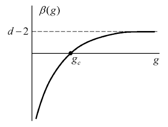
Figure 3: A typical behavior of the function $\beta(g)$ in equation (14).

According to the hypothesis of one-parameter scaling [13], the typical value of conductance $g$ obeys the renormalization group equation

$$\frac{d\ln g}{d\ln L}=\beta(g)\,,$$

where $\beta(g)=d-2$ for $g\to\infty$ and $\beta(g)=\ln g$ for $g\to 0$. For $d>2$ the function $\beta(g)$ has a root $g_{c}$ (Fig.3), which corresponds to the Anderson transition point; the critical exponent $\nu$ is determined by the derivative of $\beta(g)$ at $g_{c}$:

$$\frac{1}{\nu}=g_{c}\beta^{\prime}(g_{c})\,.$$

For $d=2+\epsilon$ the critical point is located in the region of large $g$, where expansion in $1/g$ is possible

$$\beta(g)=\epsilon+\frac{A_{1}}{g}+\frac{A_{2}}{g^{2}}+\ldots$$

It is easy to verify that retaining two first terms in (16) we have for $A_{1}<0$

$$\nu=1/\epsilon\qquad\mbox{\rm(independently of $A_{1}$)}\,,$$

while for $A_{1}=0$ and $A_{2}<0$

$$\nu=1/2\epsilon\qquad\mbox{\rm(independently of $A_{2}$)}\,,$$

i.e. in the main $\epsilon$-approximation the critical behavior is determined by the structure of expansion (16), and not by specific values of coefficients.

For $d=2$ integration of (14) with the initial condition $g=g_{0}$ at $L=a$ gives in the large $g$ region

$$g=g_{0}+A_{1}\ln(L/a)\,,$$

i.e. well-known logarithmic correction of the weak localization theory. Its existence can be controlled by the diagrammatic approach [21], confirming finiteness and negativeness of $A_{1}$. In the presence of the magnetic field, the logarithmic divergency for $L\to\infty$ is cut off at the magnetic length $l_{H}$, and absence of the contribution $\sim\ln L$ signifies disappearance of the coefficient $A_{1}$ and validity of the result (18).

According to the qualitative picture of weak localization [20, 22], the main quantum correction to a classical diffusion is related with self-intersection of trajectories, when a possibility to pass the closed loop in two opposite directions makes the quantum interference to be inevitable. If a diffusion trajectory is represented as a tube with the thickness of order the de Broglie wavelength $\lambda$, then the probability of self-intersection is determined by a ratio of the volume $v_{F}\lambda^{d-1}dt$, sweeping by the trajectory during time $dt$, to the volume $(Dt)^{d/2}$ of the region where the trajectory is localized at the instant of time $t$ ($v_{F}$ is the Fermi velocity, and $D$ is a diffusion constant). The main quantum correction $\Delta g$ to the classical conductance $g_{0}$ is determined by the total probability of self-intersection given by integration over $t$

$$-\frac{\Delta g}{g_{0}}\sim\int v_{F}\lambda^{d-1}(Dt)^{-d/2}dt\,,$$

and has logarithmic divergency at the upper limit for $d=2$ (the lower limit of integration is given by the elastic mean free time $\tau$). This divergency is cut off at the scale $\tau_{L}\sim L^{2}/D$ and leads to the logarithmic $L$ dependence.

In the presence of the magnetic field, the amplitudes of bypassing the closed loop in two opposite directions acquire the phase difference $\Delta\varphi$, which becomes comparable with $2\pi$ for the loop area of order $l_{H}^{2}$. For loops of the greater size the quantum correction is destroyed, and logarithmic divergency for $L\to\infty$ is cut off at the scale $l_{H}$. As a result, we have the complete physical picture explaining the effects of weak localization and the critical behavior for $d=2+\epsilon$.

For quasi-1D systems the closed loops are strongly oblong (Fig.4) and their area tends to zero in the limit of strictly one-dimensional systems. In the latter case, the notion of self-intersecting trajectories still survives, but the effect of destroying the quantum correction by the magnetic field disappears completely. As a result, we come to inevitable conclusion: the difference between quasi-1D and strictly 1D systems is not very essential in absence of a magnetic field, but acquires a qualitative character in presence of the field.

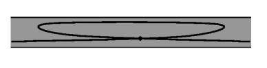
Figure 4: In quasi-1D systems, the closed loops are strongly oblong, and their area tends to zero in the limit of strictly one-dimensional systems.

Let return to the possibility to set $L=a$ in Eq.1. In fact, universal relations of such kind arise at the large length scales, while for scales of order $a$ have a certain transient behavior. If the function $F$ in Eq.1 is assumed unchanged, we can set only $L\sim a$, but not $L=a$. This difference was inessential in absence of a magnetic field, but becomes the matter of principle in presence of the field. In the latter case, the function $F$ in Eq.1 should be related not to equation (3), but with the evolution equation valid for quasi-1D systems.

4. Generalized DMPK equation

The counterpart of equation (2) in quasi-1D systems is given by the Dorokhov–Mello–Pereyra–Kumar equation [23]–[27], describing evolution of the diagonal elements of the many-channel transfer matrix.

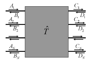
Figure 5: The many-channel transfer matrix $\hat{T}$ relates the amplitudes of plane waves on the left ($A_{n}$, $B_{n}$) and on the right ($C_{n}$, $D_{n}$) of a scatterer.

Considering the system as a set of $N$ coupled one-dimensional chains, we can treat it as an effective scatterer and describe by the transfer matrix $\hat{T}$, relating the amplitudes of waves on the left ($A_{n}e^{ikx}+B_{n}e^{-ikx}$ in the $n$-th channel) and on the right ($C_{n}e^{ikx}+D_{n}e^{-ikx}$) of the scatterer (Fig.5). Interpreting amplitudes $A_{n}$ as the components of the vector $A$, and analogously for other amplitudes, we can write the vector analog of relation (4)

$$\left(\begin{array}[]{cc}A\\ B\end{array}\right)\,=\hat{T}\left(\begin{array}[]{cc}C\\ D\end{array}\right)\,=\left(\begin{array}[]{cc}T_{11}&T_{12}\\ T_{21}&T_{22}\end{array}\right)\,\left(\begin{array}[]{cc}C\\ D\end{array}\right)\,,$$

where the transfer matrix $\hat{T}$ consists of four blocks of size $N\times N$. It allows a parametrization [25, 28]

$$\hat{T}=\left(\begin{array}[]{cc}u_{1}&0\\ 0&v_{1}\end{array}\right)\,\left(\begin{array}[]{cc}\sqrt{1+\lambda}&\sqrt{\lambda}\\ \sqrt{\lambda}&\sqrt{1+\lambda}\end{array}\right)\,\left(\begin{array}[]{cc}u&0\\ 0&v\end{array}\right)\,,$$

where $u$, $v$, $u_{1}$, $v_{1}$ are unitary matrices, and $\lambda$ is a diagonal matrix with the positive elements $\lambda_{i}$, which in particular determine the conductance

$$g_{ES}=\sum\limits_{i}\frac{1}{1+\lambda_{i}}\,$$

(in the Economou–Soukoulis definition [29, 30]). The DMPK equation describes evolution of their mutual distribution function $P\left(\lambda_{1},\lambda_{2},\ldots,\lambda_{N}\right)\equiv P\{\lambda\}$ with increasing the length $L$ of the system

$$\frac{\partial P\{\lambda\}}{\partial L}=\alpha\,\sum\limits_{i}\frac{\partial}{\partial\lambda_{i}}\left[\,\lambda_{i}(1+\lambda_{i})\,J\{\lambda\}\frac{\partial}{\partial\lambda_{i}}\,\frac{P\{\lambda\}}{J\{\lambda\}}\,\right]\,,$$

$$J\{\lambda\}=\prod\limits_{i<j}|\lambda_{i}-\lambda_{j}|^{\beta}\,,$$

where $\beta=1$ for the orthogonal ensemble (usual systems with a random potential), $\beta=2$ for the unitary ensemble (systems in the strong magnetic field), $\beta=4$ for the symplectic ensemble (systems with the strong spin-orbit interaction); the parameter $\alpha=1/\xi_{1D}$ has a sense of the inverse correlation length of the quasi-1D system. Equation (24) is obtained from the maximum entropy principle (i.e. in assumption of the maximal randomness compatible with the symmetry restrictions) and ideologically close to the random matrix theory by Wigner and Dyson [31].

In a strictly one-dimensional system one has $J\{\lambda\}=1$, and $\lambda$ coincides with the Landauer resistance $\rho$, so (24) reduces to (2).  This is quite natural, since (24) and (2) are based on analogous assumptions (compare [17] and [24]). In the paper [8] we have suggested the more general form of the DMPK equation, which reduces to (3) in the one-channel case 

$$\frac{\partial P\{\lambda\}}{\partial L}=\alpha\,\sum\limits_{i}K_{ii}\frac{\partial}{\partial\lambda_{i}}\left[\,-\gamma_{i}(1+2\lambda_{i})\,P\{\lambda\}\right.+$$

$$+\left.\lambda_{i}(1+\lambda_{i})\,J_{i}\{\lambda\}\frac{\partial}{\partial\lambda_{i}}\,\frac{P\{\lambda\}}{J_{i}\{\lambda\}}\,\right]$$

$$J_{i}\{\lambda\}=\prod\limits_{j<k}|\lambda_{j}-\lambda_{k}|^{\beta^{i}_{jk}}\,,\qquad\beta^{i}_{jk}=2K_{jk}/K_{ii}\,,\qquad$$

$$\gamma_{i}=(1-\sum_{j}K_{ij})/K_{ii}\,,\qquad$$

where the matrix $K_{ij}$ is determined by the averaged combinations of the $u$ and $v$ matrix elements. Equation (25) reduces to the usual DMPK equation in the metallic regime and provides the correct generalization beyond it. Eq.25 has the same structure for the orthogonal and unitary ensembles and allows to describe systems in the arbitrary magnetic field.

If the transverse size of a quasi-1D system is sufficiently small, then its channels are well mixed by scattering, and the approximation of equivalent channels looks reasonable, when we can set $\alpha K_{ii}=\tilde{\alpha}$, $\beta^{i}_{jk}=\beta$, $\gamma_{i}=\gamma$. Then the evolution equation is described by three parameters $\tilde{\alpha}L$, $\beta$, $\gamma$, which are in one-to-one correspondence with parameters $L/\xi$, $L_{z}/L$, $L/l_{H}$ entering equation (10),  so the first problem of Sec.2 is resolved successfully.

The second problem is also solved. Indeed, let us set $\alpha=1/\xi_{1D}$ and consider the case $L/\xi_{1D}\ll 1$, when the usual DMPK equation is valid; then conductance $g$ is determined by the ratio $L/\xi_{1D}$ (see (23,24)) and allows the expansion [37]

$$g=F\left(\,\frac{L}{\xi_{1D}}\,\right)=\frac{\xi_{1D}}{L}+B_{0}+B_{1}\frac{L}{\xi_{1D}}+\ldots$$

Substituting into (14), one can easily recover the expansion of $\beta(g)$ in the quasi-1D case

$$\beta_{1D}(g)=-1+\frac{B_{0}}{g}+\frac{2B_{1}}{g^{2}}+\ldots$$

Accepting $\langle g\rangle$ as a typical value of $g$ and following to the Shapiro scheme (Fig.1), one has

$$g^{(d)}_{bL}=b^{d-1}g^{(1)}_{bL}\,.$$

Let accept $b=1+\Delta L/L$, so that the size of the cubical system changes from $L$ to $L+\Delta L$. Increasing the length of the quasi-1D system is described by equation (14), while the increase of its transverse size is taken into account by Eq.28

$$\ln g^{(1)}_{L+\Delta L}=\ln g^{(1)}_{L}+\frac{\Delta L}{L}\beta_{1D}\left(g^{(1)}_{L}\right)\,,$$

$$\ln g^{(d)}_{L+\Delta L}=\ln g^{(1)}_{L+\Delta L}+(d-1)\frac{\Delta L}{L}\,.$$

As a result

$$\ln g^{(d)}_{L+\Delta L}=\ln g^{(d)}_{L}+\left[d-1+\beta_{1D}\left(g^{(d)}_{L}\right)\right]\,\frac{\Delta L}{L}$$

and we recover the expansion (16) for $\beta(g)=d-1+\beta_{1D}(g)$ in the $d$-dimensional case with the coefficients

$$A_{1}=B_{0}\,,\qquad A_{2}=2B_{1}\,.$$

Expansion coefficients in (26) were calculated by Mac$\rm\hat{e}$do [37] for arbitrary values of the Wigner–Dyson parameter $\beta$:

$$B_{0}=-\frac{2-\beta}{3\beta}\,,\qquad B_{1}=\frac{12-14\beta+3\beta^{2}}{45\beta^{2}}\,,$$

which leads to

$$A_{1}=-\frac{1}{3}\,,\qquad A_{2}=\frac{2}{45}\,,\qquad(\beta=1)$$

$$A_{1}=0\,,\qquad A_{2}=-\frac{2}{45}\,,\qquad(\beta=2)$$

and provides the correct structure of expansion (16) and results (17), (18) for the orthogonal and unitary ensembles respectively .

Let discuss once more the possibility to set $L=a$ in equation (1), where the function $F$ has a certain transient behavior at scales of order $a$. We indicated in [3] that such transient behavior can be excluded in accordance with the general Wilson analysis [11, 12], if the special model is chosen at small scales. Now one can see that such ”ideal model” is described by the generalized DMPK equation with the limiting transition indicated in Footnote 4.

One can see that the Shapiro scheme becomes satisfactory in the presence of the magnetic field, if the quasi-1D evolution equation is taken in the form of the generalized DMPK equation.

5. The evolution equation for $P(\rho)$

As was discussed in [3, 38], for the correct definition of conductance of finite systems it is useful to introduce semi-transparent boundaries, separating the given system from the ideal leads attached to it. In the limit of weak transparency one obtains universal equations, independent of the way how the contact resistance of the reservoir is excluded [39], which then can be extrapolated to transparency of order unity. Such definition surely refers to the system under consideration (and not to the composed system ”sample+ideal leads”) and provides the infinite value of conductance for ideal systems [38]. In the limit of weakly-transparent interfaces, the scale of all $\lambda_{i}$ increases and the Economou–Soukoulis definition of conductance (23) becomes equivalent to the definition

$$g=\frac{1}{\rho}=\sum\limits_{i}\frac{1}{\lambda_{i}}\,,$$

where conductance of each channel is taken in the Landauer form [7]. To make transition from $\lambda_{i}$ to $\rho$ let introduce the set of the ”angle” variables $\{\varphi\}=\left(\varphi_{1},\varphi_{2},\ldots\varphi_{N-1}\right)$ and make a change

$$\frac{1}{\lambda_{i}}=\frac{1}{\rho}f_{i}\{\varphi\}\,.$$

It is easy to derive for large $\lambda_{i}$

$$\rho_{ES}=\rho+\rho_{0}\,,\qquad\rho_{0}=\sum\limits_{i}f_{i}^{2}\{\varphi\}\,,$$

and obtain the inequality

$$0\leq\rho_{0}\leq 1\,,$$

following from $f_{i}\{\varphi\}\geq 0$ and $\sum_{i}f_{i}\{\varphi\}=1$. In fact, for different situations the whole range of the $\rho_{0}$ values is covered. In the metallic regime all $\lambda_{i}$ are of the same order, so $f_{i}\{\varphi\}\sim 1/N$ and $\rho_{0}\sim 1/N$, which can be arbitrary small for the large number of channels. In the strongly localized regime conductance of the system is determined by the single channel, so $f_{1}\{\varphi\}\approx 1$, $f_{i}\{\varphi\}\approx 0$ ($i\neq 1$) and $\rho_{0}\approx 1$.

The change of variables (35) is analogous to transition $x_{i}=rf_{i}\{\varphi\}$ from the Cartesian coordinates $x_{i}$ to the spherical ones. In the latter case the radius-vector $r$ has a dimension of length, while the angles $\varphi_{k}$ are dimensionless; correspondingly, a dimension of $x_{i}$ coincides with a dimension of $r$. Analogously, it is convenient to imagine that $\rho$ is a dimensional quantity, while $\lambda_{i}$ have a dimension of $\rho$. Since a dimension of each term is conserved in transformation of derivatives, the form of equation (25) in variables $\rho$, $\varphi_{k}$ can be written simply from dimensional considerations

$$\frac{\partial P}{\alpha\partial L}=\,\left[\,a_{1}\{\varphi\}\rho^{2}+a_{2}\{\varphi\}\rho\,\right]\frac{\partial^{2}P}{\partial\rho^{2}}+$$

$$+\left[\,a_{3}\{\varphi\}\rho+a_{4}\{\varphi\}\,\vphantom{\rho^{2}}\right]\frac{\partial P}{\partial\rho}+a_{5}\{\varphi\}P+$$

$$+\sum\limits_{k}\left[\,b_{k}\{\varphi\}\rho+c_{k}\{\varphi\}\,\vphantom{\rho^{2}}\right]\frac{\partial^{2}P}{\partial\rho\partial\varphi_{k}}+\sum\limits_{k}\,g_{k}\{\varphi\}\frac{\partial P}{\partial\varphi_{k}}+$$

$$+\sum\limits_{kk^{\prime}}\,h_{kk^{\prime}}\{\varphi\}\frac{\partial^{2}P}{\partial\varphi_{k}\partial\varphi_{k^{\prime}}}\,,$$

where terms with the factor $1/\rho$ are omitted . Averaging over $\varphi_{k}$ and eliminating the angle derivatives with the use of integration by parts, we arrive to

$$\frac{\partial P(\rho)}{\partial L}=\alpha\,\left[\left(C_{1}\rho^{2}+C_{2}\rho\right)\frac{\partial^{2}P(\rho)}{\partial\rho^{2}}\right.+$$

$$+\left.\left(C_{3}\rho+C_{4}\vphantom{\rho^{2}}\right)\frac{\partial P(\rho)}{\partial\rho}+C_{5}P(\rho)\right]\,.$$

Due to conservation of probability the right hand side should have a form of the full derivative; including $C_{1}$ in redefinition of $\alpha$, one has the equation

$$\frac{\partial P(\rho)}{\partial L}=\tilde{\alpha}\,\frac{\partial}{\partial\rho}\left[\left(A\rho+B\vphantom{\rho^{2}}\right)P(\rho)+\left(\rho^{2}+C\rho\right)\frac{\partial P(\rho)}{\partial\rho}\,\right]$$

which is of the same structure as (3). Two equations become identical in the result of the following transformations, carried out in [3]. Ambiguity in the conductance definition, related with exclusion of the reservoir contact resistance [39], corresponds to the change $\rho\to\rho-\rho_{0}$, where $\rho_{0}$ depends on details of a definition. This dependence is inessential in the limit of weakly-transparent boundaries, when a scale of $\rho$ increases unboundedly, while $\rho_{0}$ remains finite. It corresponds to the following change in the second term in the square bracket of (3)

$$\rho(\rho+1)\,\longrightarrow(\rho-\rho_{0})(\rho+1-\rho_{0})\longrightarrow\,\rho^{2}\,,$$

leading to the universal equation, independent of $\rho_{0}$, which can be extrapolated to a transparency of order unity. Analogous procedure for the first term in the square bracket of (3)

$$2\gamma\rho+\gamma\,\longrightarrow 2\gamma\rho+\gamma(1-2\rho_{0})\longrightarrow\,2\gamma\rho+\tau_{0}$$

is complicated by unknown behavior of the second summand in the course of the indicated procedure; so we denote it as $\tau_{0}$, bewaring of setting to be zero. The further analysis shows that $\tau_{0}$ should be considered as finite on the physical grounds. As a result, the following modification of equation (3) is practically used in the Shapiro scheme

$$\frac{\partial P(\rho)}{\partial L}=\tilde{\alpha}\,\frac{\partial}{\partial\rho}\left[\,-(2\gamma\rho+\tau_{0})P(\rho)+\rho^{2}\frac{\partial}{\partial\rho}P(\rho)\,\right].$$

The analogous procedure applied to Eq.40 leads to the same result, if we observe that the parameter $C$ is restricted by the inequality $0\leq C\leq 1$ (see Appendix 2) and cannot leads to unpredictable effects.

In the previous paper [3] we did not consider $\tau_{0}$ as an essential parameter. It arises in the course of the ill-defined extrapolation procedure to transparency of order unity and specifies the absolute scale of conductance, which is not controlled in theory. The situation is changed in the presence of the magnetic field, since $\tau_{0}$ may depend on the magnitude of the field and should be considered as an essential parameter. Therefore, the evolution equation for $P(\rho)$ is determined by three parameters $\tilde{\alpha}L$, $\gamma$, $\tau_{0}$, which are in one-to-one correspondence with parameters $L/\xi$, $L_{z}/L$, $L/l_{H}$ entering (10).

As a result, the first problem of Sec.2 is solved in the framework of equation for $P(\rho)$, but the second problem still exists. Indeed, it is easy to verify that transformation of type (13) does not allow the result $\nu=1/2\epsilon$ for any constant values of $A$, $B$, $C$ in (40). However, these coefficients can be considered as constant only in the case when distribution $P(\rho)$ is almost stationary, and the $\varphi_{k}$ distribution has a time to relax. In the quasi-1D geometry a stationary distribution $P(\rho)$ is never realized, and coefficients $A$, $B$, $C$ always contain a certain dependence on $L$. If such dependence is taken into account, there is no problem to reach the result $\nu=1/2\epsilon$ (see Appendix 3).

We can conclude, that two problems of Sec.2 can be solved on the level of the $P(\rho)$ evolution equation, if some of statements made in [3] are formulated more accurately. However, it requires the certain assumptions, which fulfil automatically on the level of the DMPK equation.

6. Transition to the $d$-dimensional case

If the quasi-1D evolution equation is accepted in the form (43), then the Shapiro scheme (Fig.1) allows a simple transition to the $d$-dimensional case. The equation for $W(g)$, corresponding to (43), is obtained by replacements $P=g^{2}W$, $\rho=1/g$ [3]

$$\frac{\partial W(g)}{\partial L}=\tilde{\alpha}\left[\,\left(2\gamma g+2g+\tau_{0}g^{2}\right)W(g)+g^{2}W_{g}^{\prime}(g)\,\right]^{\prime}_{g}\,,$$

and to solve the $d$-dimensional problem, one should find a distribution of the sum of $n=b^{d-1}$ independent random quantities with the same distribution $W(g)$: it is made by introducing the characteristic function $F(t)=\left\langle e^{igt}\right\rangle$ and raising it to the power $n$. Instead of the characteristic function it is more convenient to use the Laplace transform

$$F(\tau)=\int_{0}^{\infty}e^{-\tau g}W(g)dg\,,$$

while the indicated procedure can be realized in the differential form. Equation for $F(\tau)$ corresponding to (44) can be written for finite differences

$$F_{L+\Delta L}(\tau)=F_{L}(\tau)+\tilde{\alpha}\Delta L\left[\,\tau(\tau+\tau_{0})F^{\prime\prime}_{L}(\tau)\right.-$$

$$-\left.2\gamma\tau F^{\prime}_{L}(\tau)\right]\,.$$

Raising $F_{L}(\tau)$ to the power $n=b^{d-1}$ and setting $b=1+\Delta L/L$, we obtain the additional term $(\Delta L/L)(d\!-\!1)F_{L}\ln F_{L}$ in the right hand side of (45). As a result, the evolution equation for the $d$-dimensional system has a following form

$$\frac{\partial F(\tau)}{\partial\ln L}=\tilde{\alpha}L\left[\,\tau(\tau+\tau_{0})F^{\prime\prime}(\tau)-2\gamma\tau F^{\prime}(\tau)\right.+$$

$$+\left.pF(\tau)\ln F(\tau)\right]\,,$$

where $p=(d\!-\!1)/\tilde{\alpha}L$. The quantity $\tilde{\alpha}L$ has a sense of $L/\xi$ and evolution in $L$ for fixed $L/\xi$ leads to a stationary distribution, corresponding to large scales; in the course of this evolution parameters $\tau_{0}$, $\gamma$ and $p$ tend to constant limits and variability of the coefficients in the quasi-1D equation (40) is of no significance. Eq.46 describes the transient process due to increasing of $L$ from the atomic scale to the scales of order $\xi$, and its stationary version is of the main interest; as a result, the parameter $\tilde{\alpha}L$ looses its actuality and its role comes to the parameter $p$. Therefore, the stationary values of $\tau_{0}$, $\gamma$, $p$ are in one-to-one correspondence with parameters $L/\xi$, $L_{z}/L$, $L/l_{H}$ of Eq.10, which are maintained fixed in the limiting transition $L\to\infty$. As a result, $\xi$ increases unboundedly and all obtained distributions refer to the critical point. ”The critical distribution” discussed usually in theoretical papers (e.g. [4, 5]) corresponds to the values $L/\xi=0$, $L_{z}/L=1$, $L/l_{H}=\infty$ (in the finite magnetic field) or $L/l_{H}=0$ (in the absence of a field), which fix the critical values of parameters $\tau_{0}$, $\gamma$, $p$ for the corresponding dimension of space. For large but finite systems, any values of $L/\xi$, $L_{z}/L$, $L/l_{H}$ are accessible.

The stationary version of equation (46) was extensively studied in the paper [3]. The universal property of distributions is existence of two asymptotic regimes, log-normal for small $g$ and exponential for large $g$, while their actuality depends on the specific situation. In the metallic phase, a distribution is determined by the central Gaussian peak, while two asymptotic regimes refer to its far tails. In the critical region, the log-normal behavior is extended to a vicinity of the maximum, and practically all distribution is determined by two asymptotes. In proceeding to the localized phase, the log-normal behavior extends even more and forces out the exponential asymptotics to the region of the remote tail.

7. Conclusion

It should be clear from preceding, that the conductance distribution in the magnetic field is described by the same equations as in absence of a field. Variation of the magnetic field does not lead to any qualitative effects in the conductance distribution and only changes its quantitative characteristics, moving the system position in the three-parameter space of $\tau_{0}$, $\gamma$, $p$. This conclusion is in accordance with numerical experiments [9, 10]. The change of the distribution under variation of the field is well-known for the metallic phase: the magnetic field increases the mean value of conductance (negative magneto-resistance [40]) and diminishes its root-mean-square fluctuation [1, 2, 41] due to suppression of the Cooperon contributions.

In contrast to the previous paper [3], the quasi-1D evolution equations were established on the basis of the generalized DMPK equation, and not by a simple analogy with one-dimensional systems. It gave possibility to refine some statements of [3] and formulate them more accurately. In the spirit of [3], we did not try to estimate the parameters $\tau_{0}$, $\gamma$, $p$ for any specific situations, but studied all family of distributions in whole. The values of these parameters can be established by calculation of several moments of conductance, which is possible by the standard methods.

Appendix 1. One-dimensional evolution equation

To establish the general form of the transfer matrix, we note that amplitudes of the incident and transmitted waves are related by the scattering $S$-matrix

$$\left(\begin{array}[]{cc}B\\ C\end{array}\right)\,=S\left(\begin{array}[]{cc}A\\ D\end{array}\right)=\left(\begin{array}[]{cc}r&t^{\prime}\\ t&r^{\prime}\end{array}\right)\,\left(\begin{array}[]{cc}A\\ D\end{array}\right)\,,$$

which is defined by the amplitudes of transmission ($t$) and reflection ($r$) for waves incident from the left of scatterer, and analogous amplitudes ($t^{\prime}$ and $r^{\prime}$) for waves incident from the right. The unitarity of $S$-matrix gives

$$|r|^{2}+|t|^{2}=1\,,\quad|r^{\prime}|^{2}+|t^{\prime}|^{2}=1\,,\quad r^{*}t^{\prime}=-t^{*}r^{\prime}\,.$$

Squaring the modulus of the latter relation, one has $|r|=|r^{\prime}|$, $|t|=|t^{\prime}|$ and the elements of $S$-matrix can be written as

$$r=|r|e^{i\theta},\quad r^{\prime}=|r|e^{i\theta^{\prime}},\quad t=|t|e^{i\varphi},\quad t^{\prime}=|t|e^{i\varphi^{\prime}},$$

with the additional relation for phases

$$e^{i\theta+i\theta^{\prime}-i\varphi-i\varphi^{\prime}}=-1\,,$$

following from $(A.2)$. Rewriting $(A.1)$ in the form (4), we have

$$\hat{T}=\left(\begin{array}[]{cc}1/t&-r^{\prime}/t\\ r/t&(tt^{\prime}-rr^{\prime})/t\end{array}\right)\,=$$

$$=\left(\begin{array}[]{cc}|1/t|e^{-i\varphi}&|r/t|\,e^{-i\theta+i\varphi^{\prime}}\\ |r/t|\,e^{i\theta-i\varphi}&|1/t|\,e^{i\varphi^{\prime}}\end{array}\right)\,.$$

Introducing the Landauer resistance $\rho=|r/t|^{2}$ [7], setting $\zeta=\varphi^{\prime}-\varphi$ and shifting the origin of $\theta$, one can reduce $(A.5)$ to the form (8).

The time-reversal symmetry is in fact the invariance with respect to the complex conjugation, where $S$ transforms to $S^{*}$ and the incident and reflected waves change their places. It gives the relation $S^{*}=S^{-1}$, which leads to $S=S^{T}$ and $\varphi=\varphi^{\prime}$, if the unitary condition $S^{+}=S^{-1}$ is taken into account. The analogous, but more complicated analysis allows to establish the canonical representation (22) with the additional relations $u=v^{*}$, $u_{1}=v_{1}^{*}$ in the time-reversal case.

If a length $L$ of an one-dimensional system is increased to $L+\Delta L$, then the transfer matrices are multiplied, $\hat{T}_{L+\Delta L}=\hat{T}_{L}\hat{T}_{\Delta L}$. Accepting the form (8) for the matrix $\hat{T}_{L}$ and setting

$$\hat{T}_{\Delta L}=\left(\begin{array}[]{cc}\sqrt{1\!+\!\epsilon^{2}}\,e^{i\beta_{1}}&-i\epsilon\,e^{i\beta_{2}+i\beta_{3}}\\ i\epsilon\,e^{-i\beta_{2}}&\sqrt{1\!+\!\epsilon^{2}}\,e^{-i\beta_{1}+i\beta_{3}}\end{array}\right)\,,$$

where $\epsilon$, $\beta_{1}$, $\beta_{2}$, $\beta_{3}$ are small random quantities,  we have for the parameter $\tilde{\rho}$, corresponding to $\hat{T}_{L+\Delta L}$, in the second order in $\epsilon$

$$\tilde{\rho}=\rho-2\epsilon\sqrt{\rho(\rho+1)}\sin\psi+\epsilon^{2}(2\rho+1)\,,$$

with

$$\psi=\theta-\varphi-\zeta+\beta_{1}+\beta_{2}\,.$$

Relation $(A.7)$ differs from $(A.2)$ of [3] only by definition of the phase $\psi$, and the rest of derivation coincides with that in [3], leading to equation (3) with parameters (9).

Appendix 2. Inequality for the parameter $C$ in (40)

If $\varphi_{1}$, $\varphi_{2}$, $\ldots$, $\varphi_{N-1}$ are independent variables, then setting

$$\frac{1}{\lambda_{i}}\,=\,\frac{\varphi_{i}}{\rho}\,,\quad i=1,2,\ldots,N-1\qquad\qquad\qquad\qquad$$

$$\frac{1}{\lambda_{N}}\,=\,\frac{\varphi_{N}}{\rho}\,,\qquad\varphi_{N}=1-\varphi_{1}-\varphi_{2}-\ldots-\varphi_{N-1}$$

and coming from $\lambda_{i}$ to $\rho$, $\varphi_{1}$, $\varphi_{2}$, $\ldots$, $\varphi_{N-1}$, we obtain the following form for the first term in the right hand side of (38)

$$\left[\,\rho^{2}\sum\limits_{i=1}^{N}K_{ii}\varphi_{i}^{2}+\rho\sum\limits_{i=1}^{N}K_{ii}\varphi_{i}^{3}\,\right]\frac{\partial^{2}P}{\partial\rho^{2}}\,.$$

Since $K_{ii}\geq 0$ (see Eq.34 in [8]) and $0\leq\varphi_{i}\leq 1$, then

$$\sum\limits_{i=1}^{N}K_{ii}\varphi_{i}^{2}\,\geq\,\sum\limits_{i=1}^{N}K_{ii}\varphi_{i}^{3}\,\geq\,0\,,$$

and averaging over $\varphi_{k}$ gives $C_{1}\geq C_{2}\geq 0$ in (39) and $0\leq C\leq 1$ in (40).

Appendix 3. To estimation of the critical behavior

Multiplying (40) by $\rho$ and integrating, one has the closed equation for $\langle\rho\rangle$

$$\frac{\partial\langle\rho\rangle}{\partial L}=a\langle\rho\rangle+b$$

with $a=\tilde{\alpha}(2-A)$, $b=\tilde{\alpha}(C-B)$. Setting

$$a=a_{0}+a_{1}L\,,\qquad b=b_{0}+b_{1}L\,,$$

we have

$$\langle\rho\rangle=b_{0}L+{\textstyle\frac{1}{2}}(a_{0}b_{0}+b_{1})L^{2}+{\textstyle\frac{1}{6}}(a_{0}^{2}b_{0}+a_{0}b_{1}+2a_{1}b_{0})L^{3}+\ldots$$

and the choice $a_{0}b_{0}+b_{1}=0$ eliminates the term of order $L^{2}$. For a narrow distribution it is equivalent to disappearance of $B_{0}$ in (26) and validity of the result (18).

References

- [1] B. L. Altshuler, JETP Lett. 41, 648 (1985) [Pis’ma Zh. Eksp. Teor. Fiz.41, 530 (1985)]; B. L. Altshuler, D. E. Khmelnitskii, JETP Lett. 42, 359 (1985) [Pis’ma Zh. Eksp. Teor. Fiz. 42, 291 (1985)].
- [2] P. A. Lee, A. D. Stone, Phys. Rev. Lett. 55, 1622 (1985); P. A. Lee, A. D. Stone, H.Fukuyama, Phys. Rev. B 35, 1039 (1987).
- [3] I. M. Suslov, J. Exp. Theor. Phys. 124, 763 (2017) [Zh. Eksp. Teor. Fiz. 151, 897 (2017)].
- [4] B. Shapiro, Phys. Rev. B 34, 4394 (1986).
- [5] B. Shapiro, Phil. Mag. 56, 1031 (1987).
- [6] B. L. Altshuler, V. E. Kravtsov, I. V. Lerner, Sov. Phys. JETP 64, 1352 (1986) [Zh. Eksp. Teor. Fiz. 91, 2276 (1986)];
- [7] R. Landauer, IBM J. Res. Dev. 1, 223 (1957); Phil. Mag. 21, 863 (1970).
- [8] I. M. Suslov, arXiv: 1703.02387.
- [9] K. Slevin, T. Ohtsuki, Phys. Rev. Lett. 78, 4083 (1997).
- [10] T. Ohtsuki, K. Slevin, T. Kawarabayashi, J. Phys.: Condensed Matter 10, 11337 (1998).
- [11] K. Wilson and J. Kogut, Renormalization Group and the Epsilon Expansion (Wiley, New York, 1974).
- [12] S. Ma, Modern Theory of Critical Phenomena (Benjamin, Reading, Mass., 1976).
- [13] E. Abrahams, P. W. Anderson, D. C. Licciardello, and T. V. Ramakrishnan, Phys. Rev. Lett. 42, 673 (1979).
- [14] V. I. Melnikov, Sov. Phys. Sol. St. 23, 444 (1981).
- [15] A. A. Abrikosov, Sol. St. Comm. 37, 997 (1981).
- [16] N. Kumar, Phys. Rev. B 31, 5513 (1985).
- [17] P. Mello, Phys. Rev. B 35, 1082 (1987).
- [18] P. W. Anderson, D. J. Thouless, E. Abrahams, D. S. Fisher, Phys. Rev. B 22, 3519 (1980).
- [19] K. B. Efetov, Sov. Phys. JETP 55, 514 (1982). [Zh. Eksp. Teor. Fiz. 82, 872 (1982)]
- [20] K. B. Efetov, Supersymmetry in disorder and haos, Cambridge, University Presss, 1995, p.32–34.
- [21] L. P. Gorkov, A. I. Larkin, D. E. Khmelnitskii, Sov. Phys. JETP Lett. 30, 228 (1979). [Pis’ma Zh. Eksp. Teor. Fiz. 30, 248 (1979)]
- [22] B. L. Altshuler, A. G. Aronov, D. E. Khmelnitskii, A. I. Larkin, in Quantum Theory of Solids, ed. I. M. Lifshits, MIR Publishers, 1983.
- [23] O. N. Dorokhov, JETP Letters 36, 318 (1982).
- [24] P. A. Mello, P. Pereyra, N. Kumar, Ann. Phys. (N.Y.) 181, 290 (1988).
- [25] P. A. Mello, A. D. Stone, Phys. Rev. B 44, 3559 (1991).
- [26] A. M. S. Macedo, J. T. Chalker, Phys. Rev. B 46, 14985 (1992).
- [27] C. W. J. Beenakker, Rev. Mod. Phys. 69, 731 (1997).
- [28] P. A. Mello, J. L. Pichard, J. Phys. I 1, 493 (1991).
- [29] E. N. Economou, C. M. Soukoulis, Phys. Rev. Lett. 46, 618 (1981).
- [30] D. S. Fisher, P. A. Lee, Phys. Rev. B 23, 6851 (1981).
- [31] M. L. Mehta, Random Matrices, Academic, New York, 1991.
- [32] K. A. Muttalib, J. R. Klauder, Phys. Rev. Lett. 82, 4272 (1999).
- [33] K. A. Muttalib, V. A. Gopar, Phys. Rev. B 66, 115318 (2002).
- [34] A. Douglas, P. Marko, K. A. Muttalib, J. Phys. A: Math. Theor. 47, 125103 (2014).
- [35] K. A. Muttalib, P. Markos, P. Wolfle, Phys. Rev. B 72, 125317 (2005).
- [36] A. Douglas, K. A. Muttalib, Phys. Rev. B 80, 161102(R) (2009); arXiv: 1007.1438.
- [37] A. M. S. Macdo, Phys. Rev. B 49, 1858 (1994).
- [38] I. M. Suslov, JETP 115, 897 (2012) [Zh. Eksp. Teor. Fiz. 142, 1020 (2012)].
- [39] A. D. Stone, A. Szafer, IBM J. Res. Dev. 32, 384 (1988).
- [40] B. L. Altshuler, D. Khmelnitzkii, A. I. Larkin, P. A. Lee, Phys. Rev. B 22, 5142 (1980).
- [41] B. L. Altshuler, B. I. Shklovskii, Zh. Eksp. Teor. Fiz. 91, 220 (1986) [Sov. Phys. JETP 64, 127 (1986)].