Abstract

We calculate 3-loop master integrals for heavy quark correlators and the 3-loop QCD corrections to the $\rho$-parameter. They obey non-factorizing differential equations of second order with more than three singularities, which cannot be factorized in Mellin-$N$ space either. The solution of the homogeneous equations is possible in terms of convergent close integer power series as ${}_{2}F_{1}$ Gauß hypergeometric functions at rational argument. In some cases, integrals of this type can be mapped to complete elliptic integrals at rational argument. This class of functions appears to be the next one arising in the calculation of more complicated Feynman integrals following the harmonic polylogarithms, generalized polylogarithms, cyclotomic harmonic polylogarithms, square-root valued iterated integrals, and combinations thereof, which appear in simpler cases. The inhomogeneous solution of the corresponding differential equations can be given in terms of iterative integrals, where the new innermost letter itself is not an iterative integral. A new class of iterative integrals is introduced containing letters in which (multiple) definite integrals appear as factors. For the elliptic case, we also derive the solution in terms of integrals over modular functions and also modular forms, using $q$-product and series representations implied by Jacobi’s $\vartheta_{i}$ functions and Dedekind’s $\eta$-function. The corresponding representations can be traced back to polynomials out of Lambert–Eisenstein series, having representations also as elliptic polylogarithms, a $q$-factorial $1/\eta^{k}(\tau)$, logarithms and polylogarithms of $q$ and their $q$-integrals. Due to the specific form of the physical variable $x(q)$ for different processes, different representations do usually appear. Numerical results are also presented.

1 Introduction

Many single scale Feynman integrals arising in massless and massive multi-loop calculations in Quantum Chromodynamics (QCD) [QCD] have been found to be expressible in terms of harmonic polylogarithms (HPLs) [Remiddi:1999ew], generalized harmonic polylogarithms [Moch:2001zr, Ablinger:2013cf], cyclotomic harmonic polylogarithms [Ablinger:2011te], square-root valued iterated integrals [Ablinger:2014bra], as well as more general functions, entering the corresponding alphabet in integral iteration. After taking a Mellin transform

$${\rm\bf M}[f(x)](N)=\int_{0}^{1}dxx^{N}f(x),$$ (1.1)

they can be equivalently expressed in terms of harmonic sums [Blumlein:1998if, Vermaseren:1998uu] in the simpler examples and finite sums of different kinds in the other cases [Moch:2001zr, Ablinger:2013cf, Ablinger:2011te, Ablinger:2014bra], supplemented by special numbers like the multiple zeta values [Blumlein:2009cf] and others appearing in the limit $N\rightarrow\infty$ of the nested sums, or the value at $x=1$ of the iterated integrals in Refs. [Blumlein:1998if, Vermaseren:1998uu, Remiddi:1999ew, Moch:2001zr, Ablinger:2013cf, Ablinger:2011te, Ablinger:2014bra].

In many higher order calculations a considerable reduction of the number of integrals to be calculated is obtained using integration by parts identities (IBPs) [IBP], which allow to express all required integrals in terms of a much smaller set of so called master integrals. Differential equations satisfied by these master integrals [DEQ, Caffo:1998du] can then be obtained by taking their derivatives with respect to the parameters of the problem and inserting the IBPs in the result. What remains is to solve these differential equations, given initial or boundary conditions, if possible analytically. One way of doing this is to derive an associated system of difference equations [DIFFEQ, Ablinger:2010ty, Ablinger:2014nga, Ablinger:2015tua] after applying a mapping through a formal Taylor series or a Mellin transform. If these equations factorize to first order equations, we can use the algorithm presented in Ref. [Ablinger:2015tua] for general bases to solve these systems analytically and to find the corresponding alphabets over which the iterated integrals or nested sums are built. The final solution in $N$ and $x$ space is found by using the packages Sigma [SIG1, SIG2], EvaluateMultiSums and SumProduction [EMSSP].

However, there are physical cases where full first order factorizations cannot be obtained for either the differential equations in $x$ or the difference equations in $N$. The next level of complexity is given by non-factorizable differential or difference equations of second order. Examples of this are the massive sunrise and kite integrals [SABRY, TLSR1, Caffo:1998du, Caffo:2002ch, Laporta:2004rb, TLSR2, TLSR2a, Bailey:2008ib, Broadhurst:2008mx, TLSR3, BLOCH2, TLSR4, Adams:2014vja, Adams:2015gva, Adams:2015ydq, TLSR5, Remiddi:2016gno, Adams:2016xah, TSLR6].

In the present paper, we will address the analytic solution of typical cases of this kind, related to a series of master integrals appearing in the 3-loop corrections of the $\rho$-parameter in [Grigo:2012ji]. It turns out that these integrals are more general than those appearing in the sunrise and kite diagrams, due to the appearance of also the elliptic integral of the second kind, ${\bf E}(z)$, which cannot be transformed away. The corresponding second order differential equations have more than three singularities, as in the case of the Heun equation [HEUN]. For the sake of generality, we will seek solutions of the second order homogeneous differential equations which are given in terms of Gauß’ ${}_{2}F_{1}$ functions [GAUSS] within the class of globally bounded solutions [VANH1], cf. also [BOSTAN]. Here the parameters of the ${}_{2}F_{1}$ function are rational numbers and the argument is a rational function of $x$. The complete elliptic integrals ${\bf K}(z)$ and ${\bf E}(z)$ [TRICOMI, ELLINT, ABEL, JAC1] are special cases of this class.

The hypergeometric function obeys different relations like the Euler- and Pfaff-transformations [HYP, SLATER], the 24 Kummer solutions [KUMMER, RIEMANN] and the 15 Gauß’ contiguous relations [HYP, SLATER]. There are more special transformations for higher than first order in the argument [KUMMER, GOURSAT, VANHVID, VID2]. In the present case, equivalent ${}_{2}F_{1}$ representations are obtained by applying arithmetic triangle groups [TAKEUCHI]. The corresponding algorithm has been described in Ref. [IVH] in its present most far reaching form. The relations of this type may be useful to transform a found solution into another one, which might be particularly convenient. In the case a function space of more solutions is considered, these relations have to be exploited to check the independence of the basis elements.

The main idea of the approach presented here is to obtain the factorization of a high order scalar difference or differential equation, after uncoupling [Zuercher:94, ORESYS, NewUncouplingMethod] the corresponding linear systems, to all first order parts and its second order contributions. While the first order parts have been algorithmically solved in Ref. [Ablinger:2015tua], the treatment of second order differential equations shall be automated. The class of ${}_{2}F_{1}$ solutions has an algorithmic automation to a wide extent [IVH] and it seems that this class constitutes the next one following the iterated square-root valued letters in massive single-scale 3-loop integrals. Applying this method, we obtain the corresponding ${{}_{2}F_{1}}$ functions with (partly) fractional parameters and rational argument, and ir(rational) pre-factors, forming the new letters of the otherwise iterated integrals. These letters contain a definite integral by virtue of the integral representation of the ${{}_{2}F_{1}}$ function, which cannot be fully transformed into an integral depending on the follow-up integration variable only through its integration boundaries. In general, we have therefore to iterate new letters of this kind. Through this we obtain a complete algorithmic automation of the solution also when second order differential operators contribute, having ${}_{2}F_{1}$ solutions.

As it will be shown, in a series of cases the reduction of the ${}_{2}F_{1}$ functions to complete elliptic integrals ${\bf E}(r(z))$ and ${\bf K}(r(z))$ is possible. Therefore we also study special representations in terms of $q$-series, which have been obtained in the case of the sunrise graph, cf. [BLOCH2, Adams:2014vja, Adams:2015gva, Adams:2015ydq, Adams:2016xah], before. More general representations are needed for the integrals considered in the present paper and we describe the necessary extension.

In performing a higher loop calculation, in intermediary steps usually more complicated nested integrals and sums occur than in the final result. The various necessary decompositions of the problem that have to be performed, such as the integration by parts reduction and others, account for this in part. It appears therefore necessary to have full control on these occurring structures first, which finally may simplify in the result. Moreover, experience tells that in more general situations, more and more of these structures survive, cf. [Ablinger:2014nga] in comparison to [Vermaseren:2005qc]. If the mathematical properties of the quantities occurring are known in detail, various future calculations in the field will be more easily performed.

The paper is organized as follows. In Section 2 we present the linear systems of first order differential equations for master integrals in Ref. [Grigo:2012ji] which cannot be solved in terms of iterated integrals. We first perform a decoupling into a scalar second order equation and an associated equation for each system. Using the algorithm of Ref. [Ablinger:2015tua], the non-iterative solution both in $x$- and Mellin-$N$-space is uniquely established. In Section 3 we first determine the homogeneous solutions of the second order equations, which turn out to be ${}_{2}F_{1}$ solutions [VANH1] and obey representations in terms of weighted complete elliptic integrals of first and second kind at rational argument. In Section 4 we derive the solutions in the inhomogeneous case, which are given by iterated integrals in which some letters are given by a higher transcendental function defined by a non-iterative, i.e. definite, integral in part. We present numerical representations for $x\in[0,1]$ deriving overlapping expansions around $x=0$ and $x=1$. The methods presented apply to a much wider class of functions than the ones being discussed here specifically. These need neither to have a representation in terms of elliptic integrals, nor of just a ${}_{2}F_{1}$ function. The respective letter can be given by any multiple definite integral.

Owing to the fact that we have elliptic solutions in the present cases we may also try to cast the solution in terms of series in the nome

$$q=\exp(i\pi\tau),$$ (1.2)

where

$$\tau=i\frac{{\bf K}(1-z(x))}{{\bf K}(z(x))}\leavevmode\nobreak\ \leavevmode\nobreak\ \leavevmode\nobreak\ \leavevmode\nobreak\ \text{with}\leavevmode\nobreak\ \leavevmode\nobreak\ \leavevmode\nobreak\ \leavevmode\nobreak\ \tau\in\mathbb{H}=\left\{z\in\mathbb{C},{\sf Im}(z)>0\right\}$$ (1.3)

denotes the ratio of two complete elliptic integrals of first kind and $z(x)$ is a rational function associated to the elliptic curve of the problem. It is now interesting to see which closed form solutions the corresponding series in $q$ obey. All contributing quantities can be expressed in terms ratios of the Dedekind $\eta(\tau)$ function [DEDEKINDeta], cf. Eq. (6.14). However, various building blocks are only modular forms [KF, KOECHER, MILNE, RADEMACHER, DIAMOND, SCHOENENBERG, APOSTOL, KOEHLER, ONO, MIYAKE, SERRE, MART1] up to an additional factor of

$$\frac{1}{\eta^{k}(\tau)},\leavevmode\nobreak\ \leavevmode\nobreak\ \leavevmode\nobreak\ \leavevmode\nobreak\ k>0,\leavevmode\nobreak\ \leavevmode\nobreak\ \leavevmode\nobreak\ k\in\mathbb{N}.$$ (1.4)

We seek in particular modular forms which have a representation in terms of Lambert–Eisenstein series [LAMBERT, EISENSTEIN] and can thus be represented by elliptic polylogarithms [ELLPOL]. However, the $\eta$-factor (1.4) in general remains. Thus the occurring $q$-integrands are modulated by a $q$-factorial [SLATER, ERDELYI1] denominator.

Structures of the kind for $k>0$ are frequent even in the early literature. A prominent case is given by the invariant $J$, see e.g. [HURWITZ],

$$J=\frac{G_{2}^{3}(q)}{216000\Delta(q)}$$ (1.5)

with $G_{2}(q)$ an Eisenstein series, cf. Eq.(LABEL:eq:EISEN1), and the discriminant $\Delta$

$$\Delta(q)=(2\pi)^{12}q^{2}\prod_{k=1}^{\infty}(1-q^{2k})^{24}=(2\pi)^{12}\eta^{24}(\tau).$$ (1.6)

In the more special case considered in [BLOCH2, Adams:2014vja, Adams:2015gva, Adams:2015ydq, Adams:2016xah] terms of this kind are not present.

For the present solutions, we develop the formalism in Section 5. We discuss possible extensions of integral classes to the present case in Section 6 and of elliptic polylogarithms [ELLPOL], as has been done previously in the calculation of the two-loop sunrise and kite-diagrams [BLOCH2, Adams:2014vja, Adams:2015gva, Adams:2015ydq, Adams:2016xah]. Here the usual variable $x$ is mapped to the nome $q$, expressing all contributing functions in the new variable. This can be done for all the individual building blocks, the product of which forms the desired solution. Section 7 contains the conclusions.

In Appendix LABEL:sec:8 we briefly describe the algorithm finding for second order ordinary differential equations ${}_{2}F_{1}$ solutions with a rational function argument. In Appendix LABEL:sec:10 we present for convenience details for the necessary steps to arrive at the elliptic polylogarithmic representation in the examples of the sunrise and kite integrals [BLOCH2, Adams:2014vja, Adams:2015gva, Adams:2015ydq, Adams:2016xah]. Here we compare some results given in Refs. [BLOCH2] and [Adams:2014vja]. In Appendix LABEL:sec:11 we list a series of new sums, which simplify the recent results on the sunrise diagram of Ref. [Ananthanarayan:2016pos].

In the present paper we present the results together with all necessary technical details and we try to refer to the related mathematical literature as widely as possible, to allow a wide community of readers to apply the methods presented here to other problems.

2 The Differential Equations

The master integrals considered in this paper satisfy linear differential equations of second order

$$\left[\frac{d^{2}}{dx^{2}}+p(x)\frac{d}{dx}+q(x)\right]\psi(x)=N(x)\leavevmode\nobreak\ ,$$ (2.1)

with rational functions $r(x)=p(x),q(x)$, which may be decomposed into

$$r(x)=\sum_{k=1}^{n_{r}}\frac{b_{k}^{(r)}}{x-a_{k}^{(r)}},\leavevmode\nobreak\ \leavevmode\nobreak\ \leavevmode\nobreak\ \leavevmode\nobreak\ \leavevmode\nobreak\ a_{k}^{(r)},b_{k}^{(r)}\in\mathbb{Z}\leavevmode\nobreak\ .$$ (2.2)

The homogeneous equation is solved by the functions $\psi_{1,2}^{(0)}(x)$, which are linearly independent, i.e. their Wronskian $W$ obeys

$$W(x)=\psi_{1}^{(0)}(x)\frac{d}{dx}\psi_{2}^{(0)}(x)-\psi_{2}^{(0)}(x)\frac{d}{dx}\psi_{1}^{(0)}(x)\neq 0\leavevmode\nobreak\ .$$ (2.3)

The homogeneous Eq. (2.1) determines the well-known differential equation for $W(x)$

$$\frac{d}{dx}W(x)=-p(x)W(x)\leavevmode\nobreak\ ,$$ (2.4)

which, by virtue of (2.2), has the solution

$$W(x)=\prod_{k=1}^{n_{1}}\left(\frac{1}{x-a_{k}^{(1)}}\right)^{b_{k}^{(1)}}\leavevmode\nobreak\ ,$$ (2.5)

normalizing the functions $\psi_{1,2}^{(0)}$ accordingly. A particular solution of the inhomogeneous equation (2.1) is then obtained by Euler-Lagrange variation of constants [EULLAG]

$$\psi(x) = \leavevmode\nobreak\ \leavevmode\nobreak\ \psi_{1}^{(0)}(x)\left[C_{1}-\int dx\leavevmode\nobreak\ \psi_{2}^{(0)}(x)n(x)\right]+\psi_{2}^{(0)}(x)\left[C_{2}+\int dx\leavevmode\nobreak\ \psi_{1}^{(0)}(x)n(x)\right]\leavevmode\nobreak\ ,$$ (2.6)

with

$$n(x)=\frac{N(x)}{W(x)}$$ (2.7)

and two constants $C_{1,2}$ to be determined by special physical requirements. We will consider indefinite integrals for the solution (2.6), which allows for more singular integrands. For the class of differential equations under consideration, $N(x)$ can be expressed by harmonic polylogarithms and rational functions, $W(x)$ is a polynomial, and the functions $\psi_{1,2}^{(0)}(x)$ turn out to be higher transcendental functions, which are even expressible by complete elliptic integrals in the cases considered here. Therefore Eq. (2.6) constitutes a nested integral of known functions [Remiddi:1999ew, Moch:2001zr, Ablinger:2013cf, Ablinger:2011te, Ablinger:2014bra] and elliptic integrals at rational argument.

We consider the systems of differential equations [Grigo:2012ji] for the $O(\varepsilon^{0})$ terms of the master integrals

$$\frac{d}{dx}\left(\begin{array}[]{c}f_{8a}(x)\\ f_{9a}(x)\end{array}\right)=\left(\begin{array}[]{cc}\frac{4}{x}&\frac{6}{x}\\ \frac{4(x^{2}-3)}{x(x^{2}-9)(x^{2}-1)}&\frac{2(x^{4}-9)}{x(x^{2}-9)(x^{2}-1)}\end{array}\right)\otimes\left(\begin{array}[]{c}f_{8a}(x)\\ f_{9a}(x)\end{array}\right)+\left(\begin{array}[]{c}N_{8a}(x)\\ N_{9a}(x)\end{array}\right)$$ (2.16)

and

$$\frac{d}{dx}\left(\begin{array}[]{c}f_{8b}(x)\\ f_{9b}(x)\end{array}\right)=\left(\begin{array}[]{cc}\frac{4}{x}&\frac{2}{x}\\ \frac{4(3x^{2}-1)}{x(9x^{2}-1)(x^{2}-1)}&\frac{2(9x^{4}-1)}{x(9x^{2}-1)(x^{2}-1)}\end{array}\right)\otimes\left(\begin{array}[]{c}f_{8b}(x)\\ f_{9b}(x)\end{array}\right)+\left(\begin{array}[]{c}N_{8b}(x)\\ N_{9b}(x)\end{array}\right),$$ (2.25)

with

$$N_{8a}(x) = \frac{15(-13-16x^{2}+x^{4})}{4x}-3x(-24+x^{2})\ln(x)-18x\ln^{2}(x)$$ (2.26)

$$N_{9a}(x) = \frac{1755+1863x^{2}-1255x^{4}+157x^{6}}{12x(x^{2}-9)(x^{2}-1)}-\frac{x(324-145x^{2}+15x^{4})}{(x^{2}-9)(x^{2}-1)}\ln(x)$$ (2.27)

$$+\frac{2x(45-17x^{2}+2x^{4})}{(x^{2}-9)(x^{2}-1)}\ln^{2}(x)-\frac{16x^{3}}{3(x^{2}-9)(x^{2}-1)}\ln^{3}(x)$$

$$N_{8b}(x) = -\frac{15(-1+16x^{2}+13x^{4})}{4x}+9x(8+15x^{2})\ln(x)-18(x+6x^{3})\ln^{2}(x)$$ (2.28)

$$N_{9b}(x) = -\frac{15-397x^{2}+925x^{4}+297x^{6}}{4x(9x^{2}-1)(x^{2}-1)}+\frac{3x\left(-36+35x^{2}+195x^{4}\right)}{(9x^{2}-1)(x^{2}-1)}\ln(x)$$ (2.29)

$$+\frac{6x\left(5+37x^{2}-144x^{4}\right)}{(9x^{2}-1)(x^{2}-1)}\ln^{2}(x)+\frac{16x^{3}\left(-8+27x^{2}\right)}{(9x^{2}-1)(x^{2}-1)}\ln^{3}(x).$$

By applying decoupling algorithms [Zuercher:94, ORESYS, NewUncouplingMethod] one obtains the following scalar differential equation

$$0 = \frac{d^{2}}{dx^{2}}f_{8a}(x)+\frac{9-30x^{2}+5x^{4}}{x(x^{2}-1)(9-x^{2})}\frac{d}{dx}f_{8a}(x)-\frac{8(-3+x^{2})}{(9-x^{2})(x^{2}-1)}f_{8a}(x)$$

$$-\frac{32x^{2}}{(9-x^{2})(x^{2}-1)}\ln^{3}(x)+\frac{12(-9+13x^{2}+2x^{4})}{(9-x^{2})(x^{2}-1)}\ln^{2}(x)$$

$$-\frac{6(-54+62x^{2}+x^{4}+x^{6})}{(9-x^{2})(x^{2}-1)}\ln(x)+\frac{-1161+251x^{2}+61x^{4}+9x^{6}}{2(9-x^{2})(x^{2}-1)}$$

and the further equation

$$f_{9a}(x) = -\frac{5}{8}(-13-16x^{2}+x^{4})+\frac{x^{2}}{2}(-24+x^{2})\ln(x)+3x^{2}\ln^{2}(x)-\frac{2}{3}f_{8a}(x)$$

$$+\frac{x}{6}\frac{d}{dx}f_{8a}(x).$$

Likewise, one obtains for the second system

$$0 = \frac{d^{2}}{dx^{2}}f_{8b}(x)-\frac{1-30x^{2}+45x^{4}}{x(9x^{2}-1)(x^{2}-1)}\frac{d}{dx}f_{8b}(x)+\frac{24(-1+3x^{2})}{(9x^{2}-1)(x^{2}-1)}f_{8b}(x)$$ (2.32)

$$-\frac{32x^{2}(-8+27x^{2})}{(9x^{2}-1)(x^{2}-1)}\ln^{3}(x)+\frac{12(1-13x^{2}-216x^{4}+162x^{6})}{(9x^{2}-1)(x^{2}-1)}\ln^{2}(x)$$

$$-\frac{6(6-46x^{2}-399x^{4}+81x^{6})}{(9x^{2}-1)(x^{2}-1)}\ln(x)-\frac{61-415x^{2}+2199x^{4}+675x^{6}}{2(9x^{2}-1)(x^{2}-1)}\leavevmode\nobreak\ ,$$

$$f_{9b}(x) = 9x^{2}\left(1+6x^{2}\right)\ln^{2}(x)-\frac{9}{2}x^{2}\left(8+15x^{2}\right)\ln(x)+\frac{15}{8}\left(-1+16x^{2}+13x^{4}\right)-2f_{8b}(x)$$ (2.33)

$$+\frac{1}{2}x\frac{d}{dx}f_{8b}(x)\leavevmode\nobreak\ .$$

The above differential equations of second order contain more than three singularities. We seek solutions in terms of Gauß’ hypergeometric functions with rational arguments, following the algorithm described in Appendix LABEL:sec:8. It turns out that these differential equations have ${}_{2}F_{1}$ solutions.

Two more master integrals are obtained as integrals over the previous solutions. They obey the differential equations

$$\frac{d}{dx}f_{10a}(x) = \frac{6x\big{(}x^{2}-6\big{)}H_{0}^{2}(x)}{(x^{2}-1)^{2}}-\frac{4x\big{(}x^{2}-3\big{)}}{3(x^{2}-1)^{2}}H_{0}^{3}(x)+\frac{8}{x}\Biggr{[}H_{-1,-1,0}(x)-H_{-1,1,0}(x)-H_{1,-1,0}(x)$$ (2.34)

$$+H_{1,1,0}(x)\Biggr{]}-\frac{8x}{x^{2}-1}\left[H_{0,-1,0}(x)-H_{0,1,0}(x)\right]+\frac{x\big{[}342-51x^{2}+2\pi^{2}\big{(}x^{2}-1\big{)}\big{]}}{3(x^{2}-1)^{2}}$$

$$\times H_{0}(x)+\frac{x^{4}(165-176\zeta_{3})+8x^{2}(-105+22\zeta_{3})-585}{12(x^{2}-1)^{2}x}-\frac{2\pi^{2}}{3x}\left[H_{-1}(x)-H_{1}(x)\right]$$

$$+\frac{4}{(x^{2}-1)^{2}x}f_{8a}(x)+\frac{2\big{(}x^{2}+3\big{)}}{(x^{2}-1)^{2}x}f_{9a}(x),$$

$$\frac{d}{dx}f_{10b}(x) = -\frac{6\big{(}15x^{2}+2\big{)}}{(x^{2}-1)^{2}x}H_{0}^{2}(x)+\frac{4\big{(}4x^{4}+33x^{2}+1\big{)}}{3(x^{2}-1)^{2}x}H_{0}^{3}(x)+\frac{\big{(}8-16x^{2}\big{)}}{(x^{2}-1)x}\Biggl{[}H_{0,-1,0}(x)$$ (2.35)

$$-H_{0,1,0}(x)\Biggr{]}+\frac{8}{x}\Biggl{[}H_{-1,-1,0}(x)-2H_{-1,0,0}(x)-H_{-1,1,0}(x)-H_{1,-1,0}(x)$$

$$+2H_{1,0,0}(x)+H_{1,1,0}(x)\Biggr{]}+\frac{3\big{(}59x^{2}+38\big{)}+\pi^{2}\big{(}4x^{4}-6x^{2}+2\big{)}}{3(x^{2}-1)^{2}x}H_{0}(x)$$

$$+\frac{15-192x^{6}\zeta_{3}-8x^{2}(45+2\zeta_{3})+x^{4}(-75+208\zeta_{3})}{12(x^{2}-1)^{2}x^{3}}-\frac{2\pi^{2}}{3x}\left[H_{-1}(x)-H_{1}(x)\right]$$

$$+\frac{4}{3(x^{2}-1)^{2}x^{3}}f_{8b}(x)+\frac{2\big{(}3x^{2}+1\big{)}}{3(x^{2}-1)^{2}x^{3}}f_{9b}(x)\leavevmode\nobreak\ ,$$

with $\zeta_{k},k\in\mathbb{N},\leavevmode\nobreak\ k\geq 2$ the values of the Riemann $\zeta$-function at integer argument and the harmonic polylogarithms $H_{\vec{a}}(x)$ are defined by [Remiddi:1999ew]

$$H_{b,\vec{a}}(x) = \int_{0}^{x}dyf_{b}(y)H_{\vec{a}}(y);\leavevmode\nobreak\ \leavevmode\nobreak\ f_{b}(x)\in\left\{f_{0},f_{1},f_{-1}\right\}\equiv\left\{\frac{1}{x},\frac{1}{1-x},\frac{1}{1+x}\right\};$$ (2.36)

$$H_{\tiny\underbrace{\tiny{0,...,0}}_{k}}(x)=\frac{1}{k!}\ln^{k}(x);H_{\emptyset}(x)\equiv 1\leavevmode\nobreak\ .$$

Subsequently, we will use the shorthand notation $H_{\vec{a}}(x)\equiv H_{\vec{a}}$. The harmonic polylogarithms occurring in the inhomogeneities of Eqs. (2.34, 2.35) can be rewritten as polynomials of

$$H_{0},H_{1},H_{-1},H_{0,-1},H_{0,1},H_{0,0,-1},H_{0,0,1},H_{0,-1,-1},H_{0,-1,1},H_{0,1,-1},H_{0,1,1},$$ (2.37)

cf. [Blumlein:2003gb].

3 Solution of the homogeneous equation

In the following we will derive the solution of the homogeneous part of Eqs. (2, 2.32) as examples in detail, using the algorithm outlined in Ref. [IVH], see also Appendix LABEL:sec:8.

The homogeneous solutions of Eq. (2) read

$$\psi_{1a}^{(0)}(x) = \sqrt{2\sqrt{3}\pi}\frac{x^{2}(x^{2}-1)^{2}(x^{2}-9)^{2}}{(x^{2}+3)^{4}}{}_{2}F_{1}\biggl{[}\genfrac{.}{.}{0.0pt}{}{{\tfrac{4}{3}}\mskip 8.0mu\tfrac{5}{3}}{2};z\biggr{]}$$ (3.1)

$$\psi_{2a}^{(0)}(x) = \sqrt{2\sqrt{3}\pi}\frac{x^{2}(x^{2}-1)^{2}(x^{2}-9)^{2}}{(x^{2}+3)^{4}}{}_{2}F_{1}\biggl{[}\genfrac{.}{.}{0.0pt}{}{{\tfrac{4}{3}}\mskip 8.0mu\tfrac{5}{3}}{2};1-z\biggr{]},$$ (3.2)

with

$$z=\frac{x^{2}(x^{2}-9)^{2}}{(x^{2}+3)^{3}}\leavevmode\nobreak\ .$$ (3.3)

The ${}_{2}F_{1}$ solutions (3.1, 3.2) are close integer series [VANH1] obeying

$$b\sum_{k=0}^{\infty}\tau_{k}(c\cdot z)^{k}=\sum_{k=0}^{\infty}m_{k}z^{k},\leavevmode\nobreak\ \text{with}\leavevmode\nobreak\ \leavevmode\nobreak\ \tau_{k},b\in\mathbb{Q},\leavevmode\nobreak\ m_{k}\in\mathbb{Z},$$ (3.4)

with $c=27$. The Wronskian for this system is

$$W(x)=x(9-x^{2})(x^{2}-1).$$ (3.5)

The solutions are shown in Figure 1.

Figure 1: The homogeneous solutions (3.1, 3.2) $\psi_{1a}^{(0)}$ (dashed line) and $\psi_{2a}^{(0)}$ (full line) as functions of $x$.

Equivalent solutions are found by applying relations due to triangle groups [TAKEUCHI], see Appendix LABEL:sec:8,

$$\psi_{1b}^{(0)}(x) = \frac{\sqrt{\pi}}{4\sqrt{6}}\Biggl{\{}-(x-1)(x-3)(x+3)^{2}\sqrt{\frac{x+1}{9-3x}}{}_{2}F_{1}\biggl{[}\genfrac{.}{.}{0.0pt}{}{{\tfrac{1}{2}}\mskip 8.0mu\tfrac{1}{2}}{1};z\biggr{]}$$ (3.6)

$$+(x^{2}+3)(x-3)^{2}\sqrt{\frac{x+1}{9-3x}}{}_{2}F_{1}\biggl{[}\genfrac{.}{.}{0.0pt}{}{{\tfrac{1}{2}}\mskip 8.0mu-\tfrac{1}{2}}{1};z\biggr{]}\Biggr{\}}$$

$$\psi_{2b}^{(0)}(x) = \frac{2\sqrt{\pi}}{\sqrt{6}}\Biggl{\{}x^{2}\sqrt{(x+1)(9-3x)}{}_{2}F_{1}\biggl{[}\genfrac{.}{.}{0.0pt}{}{{\tfrac{1}{2}}\mskip 8.0mu\tfrac{1}{2}}{1};1-z\biggr{]}$$ (3.7)

$$+\frac{1}{8}\sqrt{(x+1)(9-3x)}(x-3)(x^{2}+3){}_{2}F_{1}\biggl{[}\genfrac{.}{.}{0.0pt}{}{{\tfrac{1}{2}}\mskip 8.0mu-\tfrac{1}{2}}{1};1-z\biggr{]}\Biggr{\}},$$

where

$$z(x)=-\frac{16x^{3}}{(x+1)(x-3)^{3}}\leavevmode\nobreak\ .$$ (3.8)

These solutions have the Wronskian (3.5) up to a sign but differ from those in (3.1, 3.2). The ratios of the homogeneous solutions are given by

$$\frac{\psi_{1a}^{(0)}(x)}{\psi_{1b}^{(0)}(x)} = 3^{3/4}\sqrt{\frac{\pi}{2}}$$ (3.9)

$$\frac{\psi_{2a}^{(0)}(x)}{\psi_{2b}^{(0)}(x)} = -\frac{1}{3^{3/4}}\sqrt{\frac{2}{\pi}}\leavevmode\nobreak\ .$$ (3.10)

The hypergeometric functions appearing in (3.6, 3.7) are given in terms of complete elliptic integrals [TRICOMI]

$${}_{2}F_{1}\biggl{[}\genfrac{.}{.}{0.0pt}{}{{\tfrac{1}{2}}\mskip 8.0mu\tfrac{1}{2}}{1};z\biggr{]} = \frac{2}{\pi}{\bf K}(z)$$ (3.11)

$${}_{2}F_{1}\biggl{[}\genfrac{.}{.}{0.0pt}{}{{\tfrac{1}{2}}\mskip 8.0mu-\tfrac{1}{2}}{1};z\biggr{]} = \frac{2}{\pi}{\bf E}(z)\leavevmode\nobreak\ .$$ (3.12)

Both solutions obey (3.4) with $c=16$.

Figure 2: The homogeneous solutions (3.6, 3.7) $\psi_{1b}^{(0)}$ (dashed line) and $\psi_{2b}^{(0)}$ (full line) as functions of $x$.

We also used the relation [HYP1]

$${}_{2}F_{1}\biggl{[}\genfrac{.}{.}{0.0pt}{}{{\tfrac{3}{2}}\mskip 8.0mu\tfrac{3}{2}}{2};z\biggr{]}=\frac{4}{\pi z(1-z)}\left[{\bf E}(z)-(1-z){\bf K}(z)\right],$$ (3.13)

noting that it is always possible to map a ${}_{2}F_{1}(a,b;c;x)$ function with $2a,2b,c\in\mathbb{Z},c>0$ into complete elliptic integrals. Their integral representations in Legendre’s normal form [LEGENDRE] read

$${\bf K}(z) := \int_{0}^{1}\frac{dt}{\sqrt{(1-t^{2})(1-zt^{2})}}$$ (3.14)

$${\bf E}(z) := \int_{0}^{1}dt\sqrt{\frac{1-zt^{2}}{1-t^{2}}}\leavevmode\nobreak\ .$$ (3.15)

In going from (3.1, 3.2) to (3.6, 3.7) also a contiguous relation had to be applied, leading to a linear combination of two hypergeometric functions. The solutions are shown in Figure 2.

The ratio $\psi_{1b}^{(0)}/\psi_{2b}^{(0)}$ exhibits the interesting form

$$\frac{\psi_{1b}^{(0)}(x)}{\psi_{2b}^{(0)}(x)}=-\frac{1}{3}\frac{{\bf E}(z)-r_{1}(x){\bf K}(z)}{{\bf E}(1-z)-(1-r_{1}(x)){\bf K}(1-z)}$$ (3.16)

with

$$r_{1}(x)=\frac{(x+3)^{2}(x-1)}{(x^{2}+3)(x-3)},\leavevmode\nobreak\ \leavevmode\nobreak\ \leavevmode\nobreak\ \leavevmode\nobreak\ \leavevmode\nobreak\ \text{and}\leavevmode\nobreak\ \leavevmode\nobreak\ \leavevmode\nobreak\ \leavevmode\nobreak\ \leavevmode\nobreak\ \frac{r_{1}(x)}{r_{1}(-x)}=1-z(x)\leavevmode\nobreak\ .$$ (3.17)

Whether ${}_{2}F_{1}$ solutions emerging in single scale Feynman integral calculations as solutions of differential equations for master integrals are always of the class to be reducible to complete elliptic integrals a priori is not known. However, one may use the algorithm given in Appendix LABEL:sec:8 to map a solution to one represented by elliptic integrals, if the parameters of the respective ${}_{2}F_{1}$ solution match the required pattern.

The homogeneous solutions of (2.32) read

$$\psi_{3}^{(0)}(x) = -\frac{\sqrt{1-3x}\sqrt{x+1}}{2\sqrt{2\pi}}\Biggl{[}(x+1)\left(3x^{2}+1\right){\bf E}(z)-(x-1)^{2}(3x+1){\bf K}(z)\Biggr{]}$$ (3.18)

$$\psi_{4}^{(0)}(x) = -\frac{\sqrt{1-3x}\sqrt{x+1}}{2\sqrt{2\pi}}\Biggl{[}8x^{2}{\bf K}(1-z)-(x+1)\left(3x^{2}+1\right){\bf E}(1-z)\Biggr{]},$$ (3.19)

with

$$z=\frac{16x^{3}}{(x+1)^{3}(3x-1)}\leavevmode\nobreak\ .$$ (3.20)

The argument $1-z$ appeared already in complete elliptic integrals by A. Sabry in Ref. [SABRY], Eq. (68), with $x=-\lambda$, calculating the so-called kite-integral at 2 loops, 55 years ago; see also Ref. [Laporta:2004rb], Eq. (A.11), for the sunrise-diagram and [Remiddi:2016gno], Eq. (D.18), with $x=1/\sqrt{u}$ for the kite-diagram. The latter aspect also shows the close relation between the elliptic structures appearing for both topologies, which has been mentioned in Ref. [Adams:2016xah].

Using the Legendre identity [LEGENDRE]

$${\bf K}(z){\bf E}(1-z)+{\bf E}(z){\bf K}(1-z)-{\bf K}(z){\bf K}(1-z)=\frac{\pi}{2}$$ (3.21)

one obtains the Wronskian of the system (3.18, 3.19)

$$W(x)=x(9x^{2}-1)(x^{2}-1)\leavevmode\nobreak\ ,$$ (3.22)

cf. (2.5).

The homogeneous solutions (3.18, 3.19), which are complex for $x\in[0,1]$, are shown in Figure 3. The real part of $\psi_{3}^{(0)}(x)$ has a discontinuity at $x=1/3$ moving from $-(4/9)\sqrt{2/(3\pi)}$ to $(4/9)\sqrt{2/(3\pi)}$, while Re$(\psi_{4}^{(0)}(x))$ vanishes for $x>1/3$. Likewise, Im$(\psi_{4}^{(0)}(x))$ vanishes for $0\leq x\leq 1/3$.

Figure 3: The homogeneous solutions (3.18, 3.18) $\psi_{3}^{(0)}$ (dashed lines) and $\psi_{4}^{(0)}$ (full lines) as functions of $x$; left panel: real part, right panel: imaginary part.

We finally consider the ratio $\psi_{3}^{(0)}/\psi_{4}^{(0)}$

$$\frac{\psi_{3}^{(0)}(x)}{\psi_{4}^{(0)}(x)} = -\frac{{\bf E}(z)-r_{2}(x){\bf K}(z)}{{\bf E}(1-z)-(1-r_{2}(x)){\bf K}(1-z)},$$ (3.23)

where

$$r_{2}(x)=\frac{(x-1)^{2}(3x+1)}{(x+1)(3x^{2}+1)}\leavevmode\nobreak\ \leavevmode\nobreak\ \leavevmode\nobreak\ \leavevmode\nobreak\ \leavevmode\nobreak\ \text{and}\leavevmode\nobreak\ \leavevmode\nobreak\ \leavevmode\nobreak\ \leavevmode\nobreak\ \leavevmode\nobreak\ \frac{r_{2}(x)}{r_{2}(-x)}=1-z(x)\leavevmode\nobreak\ .$$ (3.24)

This structure is the same as in (3.16, 3.17) up to the pre-factor.

The solution of the inhomogeneous equations (2, 2.32) are obtained form (2.6) specifying the constants $C_{1,2}$ by physical requirements. The previous calculation of the corresponding master integrals in [Grigo:2012ji] used expansions of the propagators [Q2EXP, Steinhauser:2000ry], obtaining series representations around $x=0$ and $x=1$. The first expansion coefficients of these will be used to determine $C_{1}$ and $C_{2}$. The inhomogeneous solutions are given by

$$\psi(x)=\psi_{1}^{(0)}(x)\left[C_{1}-I_{2}(x)\right]+\psi_{2}^{(0)}(x)\left[C_{2}+I_{1}(x)\right],$$ (3.25)

with

$$I_{1(2)}(x)=\int dx\psi_{1(2)}(x)\frac{N(x)}{W(x)}\leavevmode\nobreak\ .$$ (3.26)

Eq. (3.25) is an integral which cannot be represented within the class of iterative integrals. It therefore requires a generalization. We present this in Section 4. Efficient numerical representations using series expansions are given in Section 5.

4 Iterated Integrals over Definite Integrals

The elliptic integrals (3.14, 3.15) cannot be rewritten as integrals in which their argument $x$ only appears in one of their integral boundaries. Therefore, the integrals of the type of Eq. (3.25) do not belong to the iterative integrals of the type given in Refs. [Remiddi:1999ew, Ablinger:2011te, Ablinger:2013cf, Ablinger:2014bra] and generalizations thereof to general alphabets, which have the form

$$H_{b,\vec{a}}(x)=\int_{0}^{x}dyf_{b}(y)H_{\vec{a}}(y)\leavevmode\nobreak\ .$$ (4.1)

For a given difference equation, associated to a corresponding differential equation, the algorithms of [SIG1, SIG2] based on [SIGBASE] allow to decide whether or not the recurrence is first order factorizable. In the first case the corresponding nested sum-product structure is returned. In the case the problem is not first order factorizable, integrals will be introduced whose integrands depend on variables that cannot be moved to the integration boundaries and over which one will integrate by later integrals. This is the case if the corresponding quantity obeys a differential equation of order $m\geq 2$, not being reducible to lower orders. Examples of this kind are irreducible Gauß’ ${}_{2}F_{1}$ functions, to which also the complete elliptic integrals ${\bf E}(z)$ and ${\bf K}(z)$ belong.

The new iterative integrals are given by

$$\mathbb{H}_{a_{1},...,a_{m-1};\{a_{m};F_{m}(r(y_{m}))\},a_{m+1},...,a_{q}}(x) = \int_{0}^{x}dy_{1}f_{a_{1}}(y_{1})\int_{0}^{y_{1}}dy_{2}...\int_{0}^{y_{m-1}}dy_{m}f_{a_{m}}(y_{m})F_{m}[r(y_{m})]$$ (4.2)

$$\times H_{a_{m+1},...,a_{q}}(y_{m+1}),$$

and cases in which more than one definite integral $F_{m}$ appears. Here the $f_{a_{i}}(y)$ are the usual letters of the different classes considered in [Remiddi:1999ew, Ablinger:2011te, Ablinger:2013cf, Ablinger:2014bra] multiplied by hyperexponential pre-factors

$$r(y)y^{r_{1}}(1-y)^{r_{2}},\leavevmode\nobreak\ \leavevmode\nobreak\ \leavevmode\nobreak\ \leavevmode\nobreak\ r_{i}\in\mathbb{Q},\leavevmode\nobreak\ r(y)\in\mathbb{Q}[y]$$ (4.3)

and $F[r(y)]$ is given by

$$F[r(y)]=\int_{0}^{1}dzg(z,r(y)),\leavevmode\nobreak\ \leavevmode\nobreak\ \leavevmode\nobreak\ r(y)\in\mathbb{Q}[y],$$ (4.4)

such that the $y$-dependence cannot be transformed into one of the integration boundaries completely. We have chosen here $r(y)$ as a rational function because of concrete examples in this paper, which, however, is not necessary. Specifically we have

$$F[r(y)] = {}_{2}F_{1}\biggl{[}\genfrac{.}{.}{0.0pt}{}{a\mskip 8.0mub}{c};r(y)\biggr{]}=\frac{\Gamma(c)}{\Gamma(b)\Gamma(c-b)}\int_{0}^{1}dzz^{b}(1-z)^{c-b-1}\left(1-r(y)z\right)^{-a},$$ (4.5)

$$\hskip 227.62204ptr(y)\in\mathbb{Q}[y],a,b,c\in\mathbb{Q}.$$

The new iterated integral (4.2) is not limited to the emergence of the functions (4.5). Multiple definite integrals are allowed as well. They emerge e.g. in the case of Appell-functions [HYP, SLATER] and even more involved higher functions. These integrals also obey relations of the shuffle type w.r.t. their letters $f_{a_{m}}(y_{m})(F_{m}[r(y_{m})])$, cf. e.g. [SHUF, Blumlein:2003gb].

Within the analyticity region of the problem one may derive series expansions of the corresponding solutions around special values, e.g. $x=0,x=1$ and other values to map out the function for its whole argument range. In many cases, one will even find convergent, widely overlapping representations, which are highly accurate and provide a numerical solution in terms of a finite number of analytic expansion coefficients. We apply this method to the solution of the differential equations in Section 2 in the following section and return to the construction of a closed form analytic representation using $q$-series and Dedekind $\eta$ functions in Section 6.

5 The Solution of the Inhomogeneous Equation by Series Expansion

The inhomogeneous solutions of type (3.25) can be expanded into series around $x=0$ and $x=1$ analytically using computer algebra packages like Mathematica or maple. One either obtains Taylor series or superpositions of Taylor series times a factor $\ln^{k}(x),k\in\mathbb{N}$. For all solutions both expansions have a wide overlap and one may obtain in this way a highly accurate representation of all solutions in the complete region $x\in[0,1]$.

In the following we present the first terms of the series expansion for the functions $f_{8(9,10),a(b)}(x)$ around $x=0$ and $x=1$.

For $f_{8a}$ we obtain

$$f_{8a}(x) = -\sqrt{3}\Biggl{[}\pi^{3}\Biggl{(}\frac{35x^{2}}{108}-\frac{35x^{4}}{486}-\frac{35x^{6}}{4374}-\frac{35x^{8}}{13122}-\frac{70x^{10}}{59049}-\frac{665x^{12}}{1062882}\Biggr{)}+\Biggl{(}12x^{2}-\frac{8x^{4}}{3}$$ (5.1)

$$-\frac{8x^{6}}{27}-\frac{8x^{8}}{81}-\frac{32x^{10}}{729}-\frac{152x^{12}}{6561}\Biggr{)}{\sf Im}\Biggl{[}\text{Li}_{3}\left(\frac{e^{-\frac{i\pi}{6}}}{\sqrt{3}}\right)\Biggr{]}\Biggr{]}-\pi^{2}\Biggl{(}1+\frac{x^{4}}{9}-\frac{4x^{6}}{243}-\frac{46x^{8}}{6561}$$

$$-\frac{214x^{10}}{59049}-\frac{5546x^{12}}{2657205}\Biggr{)}-\Biggl{(}-\frac{3}{2}-\frac{x^{4}}{6}+\frac{2x^{6}}{81}+\frac{23x^{8}}{2187}+\frac{107x^{10}}{19683}+\frac{2773x^{12}}{885735}\Biggr{)}\psi^{(1)}\left(\frac{1}{3}\right)$$

$$-\sqrt{3}\pi\Biggl{(}\frac{x^{2}}{4}-\frac{x^{4}}{18}-\frac{x^{6}}{162}-\frac{x^{8}}{486}-\frac{2x^{10}}{2187}-\frac{19x^{12}}{39366}\Biggr{)}\ln^{2}(3)-\Biggl{[}33x^{2}-\frac{5x^{4}}{4}-\frac{11x^{6}}{54}$$

$$-\frac{19x^{8}}{324}-\frac{751x^{10}}{29160}-\frac{2227x^{12}}{164025}+\pi^{2}\Biggl{(}\frac{4x^{2}}{3}-\frac{8x^{4}}{27}-\frac{8x^{6}}{243}-\frac{8x^{8}}{729}-\frac{32x^{10}}{6561}-\frac{152x^{12}}{59049}\Biggr{)}$$

$$+\Biggl{(}-2x^{2}+\frac{4x^{4}}{9}+\frac{4x^{6}}{81}+\frac{4x^{8}}{243}+\frac{16x^{10}}{2187}+\frac{76x^{12}}{19683}\Biggr{)}\psi^{(1)}\left(\frac{1}{3}\right)\Biggr{]}\ln(x)+\frac{135}{16}+19x^{2}$$

$$-\frac{43x^{4}}{48}-\frac{89x^{6}}{324}-\frac{1493x^{8}}{23328}-\frac{132503x^{10}}{5248800}-\frac{2924131x^{12}}{236196000}-\Biggl{(}\frac{x^{4}}{2}-12x^{2}\Biggr{)}\ln^{2}(x)$$

$$-2x^{2}\ln^{3}(x)+O\left(x^{14}\ln(x)\right)$$

around $x=0$. Here we also applied a series of relations for $\psi^{(k)}$-functions at rational argument, cf. Ref. [Ablinger:2011te].

Likewise, one may expand around $y=1-x=0$. In this case, we can rewrite the inhomogeneous solution given in (3.25) as

$$\psi(y)=\psi_{1}^{(0)}(y)\left[\overline{C}_{1}-\bar{I}_{2}(y)\right]+\psi_{2}^{(0)}(y)\left[\overline{C}_{2}+\bar{I}_{1}(y)\right],$$ (5.2)

with

$$\bar{I}_{1(2)}(x) = \int dy\leavevmode\nobreak\ \psi_{1(2)}^{(0)}(y)\frac{N(y)}{W(y)},$$ (5.3)

$$W(y) = \psi_{1}^{(0)}(y)\frac{d}{dy}\psi_{2}^{(0)}(y)-\psi_{2}^{(0)}(y)\frac{d}{dy}\psi_{1}^{(0)}(y).$$ (5.4)

One obtains

$$f_{8a}(x) = \frac{275}{12}+\frac{10}{3}y-25y^{2}+\frac{4}{3}y^{3}+\frac{11}{12}y^{4}+y^{5}+\frac{47}{96}y^{6}+\frac{307}{960}y^{7}+\frac{19541}{80640}y^{8}+\frac{22133}{120960}y^{9}$$ (5.5)

$$+\frac{1107443}{7741440}y^{10}+\frac{96653063}{851558400}y^{11}+\frac{3127748803}{34062336000}y^{12}$$

$$+7\Biggl{(}2y^{2}-y^{3}-\frac{1}{8}y^{4}-\frac{1}{64}y^{6}-\frac{1}{128}y^{7}-\frac{3}{512}y^{8}-\frac{1}{256}y^{9}-\frac{47}{16384}y^{10}$$

$$-\frac{69}{32768}y^{11}-\frac{421}{262144}y^{12}\Biggr{)}\zeta_{3}+O(y^{13})\leavevmode\nobreak\ .$$

The solution of Eq. (2) around $x=0$ reads

$$f_{9a}(x) = \sqrt{3}\Biggl{(}4x^{2}+\frac{8x^{6}}{81}+\frac{16x^{8}}{243}+\frac{32x^{10}}{729}+\frac{608x^{12}}{19683}\Biggr{)}{\sf Im}\Biggl{(}\text{Li}_{3}\Biggl{(}\frac{e^{-\frac{i\pi}{6}}}{\sqrt{3}}\Biggr{)}\Biggr{]}+\sqrt{3}\pi^{3}\Biggl{(}\frac{35x^{2}}{324}$$ (5.6)

$$+\frac{35x^{6}}{13122}+\frac{35x^{8}}{19683}+\frac{70x^{10}}{59049}+\frac{1330x^{12}}{1594323}\Biggr{)}+\sqrt{3}\pi\Biggl{(}\frac{x^{2}}{12}+\frac{x^{6}}{486}+\frac{x^{8}}{729}+\frac{2x^{10}}{2187}+\frac{38x^{12}}{59049}\Biggr{)}$$

$$\times\ln^{2}(3)+\pi^{2}\Biggl{(}\frac{2}{3}-\frac{2x^{2}}{9}+\frac{4x^{4}}{81}+\frac{8x^{6}}{729}+\frac{128x^{8}}{19683}+\frac{262x^{10}}{59049}+\frac{25604x^{12}}{7971615}\Biggr{)}+\Biggl{(}-1+\frac{x^{2}}{3}$$

$$-\frac{2x^{4}}{27}-\frac{4x^{6}}{243}-\frac{64x^{8}}{6561}-\frac{131x^{10}}{19683}-\frac{12802x^{12}}{2657205}\Biggr{)}\psi^{(1)}\left(\frac{1}{3}\right)+\Biggl{(}3x^{2}+\frac{x^{4}}{3}+\frac{11x^{6}}{162}+\frac{19x^{8}}{486}$$

$$+\frac{751x^{10}}{29160}+\frac{8908x^{12}}{492075}+\pi^{2}\Biggl{(}\frac{4x^{2}}{9}+\frac{8x^{6}}{729}+\frac{16x^{8}}{2187}+\frac{32x^{10}}{6561}+\frac{608x^{12}}{177147}\Biggr{)}+\Biggl{[}-\frac{2x^{2}}{3}-\frac{4x^{6}}{243}$$

$$-\frac{8x^{8}}{729}-\frac{16x^{10}}{2187}-\frac{304x^{12}}{59049}\Biggr{)}\psi^{(1)}\left(\frac{1}{3}\right)\Biggr{]}\log(x)+\frac{5}{2}-\frac{11x^{2}}{6}-\frac{5x^{4}}{12}-\frac{14x^{6}}{243}-\frac{1151x^{8}}{34992}$$

$$-\frac{109973x^{10}}{5248800}-\frac{2523271x^{12}}{177147000}-2x^{2}\log^{2}(x)+\frac{2}{3}x^{2}\log^{3}(x)+O\left(x^{14}\ln(x)\right)\leavevmode\nobreak\ .$$

The corresponding expansion around $x=1$ is given by

$$f_{9a}(x) = \frac{5}{3}+\frac{2}{3}y+\frac{2}{3}y^{2}+\frac{1}{2}y^{3}+\frac{1}{3}y^{4}-\frac{11}{480}y^{5}+\frac{13}{1920}y^{6}-\frac{2461}{120960}y^{7}-\frac{3701}{241920}y^{8}$$ (5.7)

$$-\frac{76627}{4644864}y^{9}-\frac{1289527}{92897280}y^{10}-\frac{635723359}{51093504000}y^{11}-\frac{13482517}{1261568000}y^{12}$$

$$+7\Biggl{(}-\frac{2}{3}y-\frac{1}{6}y^{2}+\frac{1}{4}y^{3}+\frac{1}{64}y^{5}+\frac{1}{256}y^{6}+\frac{1}{256}y^{7}+\frac{1}{512}y^{8}+\frac{25}{16384}y^{9}+\frac{65}{65536}y^{10}$$

$$+\frac{99}{131072}y^{11}+\frac{145}{262144}y^{12}\Biggr{)}\zeta_{3}+O\left(y^{13}\right)\leavevmode\nobreak\ .$$

Here the integration constants $C_{1,2}$ and $\overline{C}_{1,2}$ are

$$C_{1} = \frac{35\pi^{3}}{72}+18{\sf Im}\left[{\rm Li}_{3}\left(-\frac{e^{5i\pi/6}}{\sqrt{3}}\right)\right]+\frac{2\pi^{2}\ln(3)}{\sqrt{3}}+\frac{3}{8}\pi\ln^{2}(3)$$ (5.8)

$$+\frac{\sqrt{3}}{16}\left[25-2\ln(3)\left(45+8\psi^{(1)}\left(\frac{1}{3}\right)\right)\right]$$

$$C_{2} = -\left[\frac{135}{16}-\pi^{2}+\frac{3}{2}\psi^{(1)}\left(\frac{1}{3}\right)\right]\left(-\frac{2\pi}{9\sqrt{3}}\right)$$ (5.9)

$$\overline{C}_{1} = \frac{275}{32}\pi$$ (5.10)

$$\overline{C}_{2} = \frac{275}{64}-\frac{275}{48}\ln(2)-\frac{7}{3}\zeta_{3}\leavevmode\nobreak\ .$$ (5.11)

The solution of (2.34) is an integral containing the functions $f_{8a}(x)$ and $f_{9a}(x)$. Its series around $x=0$ reads

$$f_{10a}(x) = \sqrt{3}\Biggl{(}-12x^{2}-\frac{22x^{4}}{3}-\frac{148x^{6}}{27}-\frac{359x^{8}}{81}-\frac{13652x^{10}}{3645}-\frac{21370x^{12}}{6561}\Biggr{)}$$ (5.12)

$$\times{\sf Im}\Biggl{[}\text{Li}_{3}\left(-\frac{(-1)^{5/6}}{\sqrt{3}}\right)\Biggr{]}+\Biggl{(}6+\frac{22x^{2}}{3}+\frac{11x^{4}}{3}+\frac{22x^{6}}{9}+\frac{11x^{8}}{6}+\frac{22x^{10}}{15}+\frac{11x^{12}}{9}\Biggr{)}\zeta_{3}$$

$$+\pi^{2}\Biggl{(}\frac{7x^{2}}{6}+\frac{13x^{4}}{72}-\frac{x^{6}}{486}-\frac{12739x^{8}}{209952}-\frac{245263x^{10}}{2952450}-\frac{1950047x^{12}}{21257640}\Biggr{)}$$

$$+\sqrt{3}\pi^{3}\Biggl{(}-\frac{35x^{2}}{108}-\frac{385x^{4}}{1944}-\frac{1295x^{6}}{8748}-\frac{12565x^{8}}{104976}-\frac{23891x^{10}}{236196}-\frac{373975x^{12}}{4251528}\Biggr{)}$$

$$+\sqrt{3}\pi\Biggl{(}-\frac{x^{2}}{4}-\frac{11x^{4}}{72}-\frac{37x^{6}}{324}-\frac{359x^{8}}{3888}-\frac{3413x^{10}}{43740}-\frac{10685x^{12}}{157464}\Biggr{)}\ln^{2}(3)$$

$$+\Biggl{(}\frac{2\pi^{2}}{3}-x^{2}+\frac{7x^{6}}{81}+\frac{4825x^{8}}{34992}+\frac{76078x^{10}}{492075}-\frac{x^{4}}{12}+\frac{561323x^{12}}{3542940}\Biggr{)}\psi^{(1)}\left(\frac{1}{3}\right)$$

$$+\Biggl{[}-x^{4}-\frac{32x^{6}}{27}-\frac{761x^{8}}{648}-\frac{3251x^{10}}{2916}-\frac{27455x^{12}}{26244}+\pi^{2}\Biggl{(}-\frac{5x^{2}}{3}-\frac{53x^{4}}{54}-\frac{175x^{6}}{243}$$

$$-\frac{1679x^{8}}{2916}-\frac{15839x^{10}}{32805}-\frac{49301x^{12}}{118098}\Biggr{)}+\Biggl{(}2x^{2}+\frac{11x^{4}}{9}+\frac{74x^{6}}{81}+\frac{359x^{8}}{486}+\frac{6826x^{10}}{10935}$$

$$+\frac{10685x^{12}}{19683}\Biggr{)}\psi^{(1)}\left(\frac{1}{3}\right)\Biggr{]}\ln(x)-\frac{19\pi^{4}}{72}-\frac{1}{2}\psi^{(1)}\left(\frac{1}{3}\right)^{2}+\frac{3x^{4}}{2}+\frac{245x^{6}}{162}+\frac{31723x^{8}}{23328}$$

$$+\frac{634597x^{10}}{524880}+\frac{10219913x^{12}}{9447840}+O\left(x^{14}\ln(x)\right)\leavevmode\nobreak\ .$$

Likewise, one obtains the expansion around $x=1$, which is given by

$$f_{10a}(x) = -\frac{11\pi^{4}}{45}+\frac{4\ln^{4}(2)}{3}-\frac{4}{3}\pi^{2}\ln^{2}(2)+32\text{Li}_{4}\left(\frac{1}{2}\right)+\Bigg{[}6+3y-2y^{2}-\frac{13y^{3}}{8}-\frac{163y^{4}}{128}$$

$$-\frac{631y^{5}}{640}-\frac{1213y^{6}}{1536}-\frac{2335y^{7}}{3584}-\frac{36247y^{8}}{65536}-\frac{47221y^{9}}{98304}-\frac{69631y^{10}}{163840}-\frac{1100145y^{11}}{2883584}$$

$$-\frac{544987y^{12}}{1572864}-\frac{1082435y^{13}}{3407872}\Biggr{]}\zeta_{3}+\frac{5y^{2}}{2}+\frac{7y^{3}}{4}+\frac{2363y^{4}}{1728}+\frac{1867y^{5}}{1728}+\frac{2293073y^{6}}{2592000}$$

$$+\frac{71317y^{7}}{96000}+\frac{8080140871y^{8}}{12644352000}+\frac{31879816079y^{9}}{56899584000}+\frac{255571071379y^{10}}{512096256000}$$

$$+\frac{1844349403987y^{11}}{4096770048000}+\frac{13424123319977921y^{12}}{32716805603328000}+\frac{2056360866308893y^{13}}{5452800933888000}+O(y^{13})$$

with

$$C_{3} = -\frac{19}{72}\pi^{4}+\frac{2}{3}\pi^{2}\psi^{(1)}\left(\frac{1}{3}\right)-\frac{1}{2}\psi^{(1)}\left(\frac{1}{3}\right)^{2}+6\zeta_{3}$$ (5.14)

$$\overline{C}_{3} = 9\zeta_{4}-6\zeta_{3}-2{\sf B}_{4},$$ (5.15)

with [Broadhurst:1991fi]

$${\sf B}_{4} = -4\zeta_{2}\ln^{2}(2)+\frac{2}{3}\ln^{4}(2)-\frac{13}{2}\zeta_{4}+16{\rm Li}_{4}\left(\frac{1}{2}\right),$$ (5.16)

as integration constants in this case.

The series expansion of the solution of Eq. (2.32) is given by

$$f_{8b}(x) = -\Biggl{\{}\frac{145}{48}-19x^{2}-\frac{261}{16}x^{4}+\frac{19}{12}x^{6}+\frac{4157}{288}x^{8}+\frac{510593}{7200}x^{10}+\frac{13208647}{36000}x^{12}$$

$$+\left(\frac{1}{2}+\frac{9}{2}x^{4}-6x^{6}-23x^{8}-107x^{10}-\frac{2773}{5}x^{12}\right)\zeta_{2}$$

$$+2x^{2}\left(-1+2x^{2}+2x^{4}+6x^{6}+24x^{8}+114x^{10}\right)\zeta_{3}$$

$$-2x^{2}\left(-1-14x^{2}+4x^{4}+12x^{6}+48x^{8}+228x^{10}\right)\ln^{3}(x)$$

$$-\frac{1}{10}x^{2}\left(120+585x^{2}+120x^{4}+460x^{6}+2140x^{8}+11092x^{10}\right)\ln^{2}(x)$$

$$+\Biggl{[}(33x^{2}+\frac{201}{4}x^{4}+\frac{29}{2}x^{6}+\frac{307}{12}x^{8}+\frac{7927}{120}x^{10}+\frac{14107}{75}x^{12}$$

$$-6x^{2}\Biggl{(}-1+2x^{2}+2x^{4}+6x^{6}+24x^{8}+114x^{10}\Biggr{)}\zeta_{2}\Biggr{]}\ln(x)+O\left(x^{14}\ln^{3}(x)\right)\Biggr{\}}\leavevmode\nobreak\ .$$

The solution of Eq. (2.33) reads

$$f_{9b}(x) = -\frac{95}{12}+\frac{131}{2}x^{2}+\frac{99}{2}x^{4}+\frac{53}{6}x^{6}+\frac{5999}{144}x^{8}+\frac{196621}{800}x^{10}+\frac{14055067}{9000}x^{12}$$ (5.18)

$$+\left(-1+3x^{2}-6x^{4}-12x^{6}-64x^{8}-393x^{10}-\frac{12802}{5}x^{12}\right)\zeta_{2}$$

$$+2\left(x^{2}+2x^{6}+12x^{8}+72x^{10}+456x^{12}\right)\zeta_{3}$$

$$-2\left(x^{2}+4x^{6}+24x^{8}+144x^{10}+912x^{12}\right)\ln^{3}(x)$$

$$+\left(24x^{2}+96x^{4}-24x^{6}-128x^{8}-786x^{10}-\frac{25604}{5}x^{12}\right)\ln^{2}(x)$$

$$+\Biggl{[}-81x^{2}-126x^{4}+\frac{5}{2}x^{6}+\frac{31}{6}x^{8}-\frac{633}{40}x^{10}-\frac{26762}{75}x^{12}$$

$$-6\left(x^{2}+2x^{6}+12x^{8}+72x^{10}+456x^{12}\right)\zeta_{2}\Biggr{]}\ln(x)+O\left(x^{14}\ln^{3}(x)\right)\leavevmode\nobreak\ .$$

Here the constants in (3.25) have been fixed by comparing to the first expansion coefficients in [Grigo:2012ji]

$$C_{1} = -\frac{1}{24}\left[2i\pi(145+4\pi^{2})+3(165+16\zeta_{3})\right]$$ (5.19)

$$C_{2} = -\frac{1}{12}\pi(145+4\pi^{2})={\sf Im}(C_{1})\leavevmode\nobreak\ .$$ (5.20)

The solution of (2.35) is given as an integral containing $f_{8(9)b}(x)$ with the constant

$$C_{3} = 3\zeta_{4}+6\zeta_{3}$$ (5.21)

and reads

$$f_{10b}(x) = 3\zeta_{4}-4x^{2}+\frac{7}{4}x^{4}-\frac{553}{81}x^{6}-\frac{87587}{1728}x^{8}-\frac{9136091}{33750}x^{10}-\frac{236649223}{162000}x^{12}$$

$$+\left(-6x^{2}-\frac{1}{2}x^{4}+\frac{46}{3}x^{6}+\frac{1957}{24}x^{8}+\frac{30907}{75}x^{10}+\frac{40103}{18}x^{12}\right)\zeta_{2}$$

$$+\Biggl{[}12x^{2}-\frac{15}{2}x^{4}-\frac{257}{9}x^{6}-\frac{3613}{48}x^{8}-\frac{103577}{500}x^{10}-\frac{1039019}{1800}x^{12}$$

$$+\left(8x^{2}+16x^{4}+\frac{116}{3}x^{6}+128x^{8}+\frac{2708}{5}x^{10}+\frac{8062}{3}x^{12}\right)\zeta_{2}\Biggr{]}\ln(x)$$

$$+\left(-12x^{2}-x^{4}+\frac{92}{3}x^{6}+\frac{1957}{12}x^{8}+\frac{61814}{75}x^{10}+\frac{40103}{9}x^{12}\right)\ln^{2}(x)$$

$$+\left(\frac{16}{3}x^{2}+\frac{32}{3}x^{4}+\frac{232}{9}x^{6}+\frac{256}{3}x^{8}+\frac{5416}{15}x^{10}+\frac{16124}{9}x^{12}\right)\ln^{3}(x)$$

$$+\left(6+4x^{2}-2x^{4}-\frac{32}{3}x^{6}-41x^{8}-\frac{896}{5}x^{10}-\frac{2684}{3}x^{12}\right)\zeta_{3}+O\left(x^{14}\ln^{3}(x)\right)\leavevmode\nobreak\ .$$

The corresponding solutions around $x=1$ have the expansions

$$f_{8b}(x) = \frac{275}{12}+10y-71y^{2}+12y^{3}+\frac{57}{4}y^{4}+18y^{5}-\frac{1079}{160}y^{6}-\frac{621}{320}y^{7}-\frac{30967}{80640}y^{8}+\frac{3449}{24192}y^{9}$$ (5.23)

$$+\frac{13850687}{38707200}y^{10}+\frac{81562673}{170311680}y^{11}+\frac{6586514681}{11354112000}y^{12}$$

$$+7\Biggl{(}2y^{2}-3y^{3}+\frac{7}{8}y^{4}-\frac{1}{64}y^{6}-\frac{3}{128}y^{7}-\frac{15}{512}y^{8}-\frac{9}{256}y^{9}-\frac{687}{16384}y^{10}-\frac{1647}{32768}y^{11}$$

$$-\frac{15933}{262144}y^{12}\Biggr{)}\zeta_{3}+O\left(y^{13}\right)$$

$$f_{9b}(x) = \frac{5}{3}+2y+2y^{2}+\frac{3}{2}y^{3}-\frac{3}{2}y^{4}-\frac{171}{160}y^{5}-\frac{577}{640}y^{6}-\frac{35851}{40320}y^{7}-\frac{77957}{80640}y^{8}-\frac{1726163}{1548288}y^{9}$$ (5.24)

$$-\frac{41342669}{30965760}y^{10}-\frac{27949201859}{17031168000}y^{11}+\frac{6932053241}{2838528000}y^{12}$$

$$+7\Biggl{(}-2y+\frac{5}{2}y^{2}-\frac{1}{4}y^{3}+\frac{(3}{64}y^{5}+\frac{(17}{256}y^{6}+\frac{21}{256}y^{7}+\frac{5}{512}y^{8}+\frac{1995}{16384}y^{9}+\frac{9873}{65536}y^{10}$$

$$+\frac{24741}{131072}y^{11}-\frac{15933}{65536}y^{12}\Biggr{)}\zeta_{3}+O\left(y^{13}\right).$$

$$f_{10b}(x) = 2{\sf B}_{4}-9\zeta_{4}+\frac{5}{2}y^{2}+\frac{13}{4}y^{3}+\frac{6251}{1728}y^{4}+\frac{6721}{1728}y^{5}+\frac{10775573}{2592000}y^{6}+\frac{142659}{32000}y^{7}$$ (5.25)

$$+\frac{60860651591}{12644352000}y^{8}+\frac{298199146349}{56899584000}y^{9}+\frac{1475031521177}{256048128000}y^{10}+\frac{26211821446117}{4096770048000}y^{11}$$

$$+\frac{235080972861513791}{32716805603328000}y^{12}+\Biggl{[}6+9y+y^{2}-\frac{11}{8}y^{3}-\frac{307}{128}y^{4}-\frac{1893}{640}y^{5}-\frac{5137}{1536}y^{6}$$

$$-\frac{13179}{3584}y^{7}-\frac{263063}{65536}y^{8}-\frac{431519}{98304}y^{9}-\frac{395741}{81920}y^{10}-\frac{15466743}{2883584}y^{11}$$

$$-\frac{9465637}{1572864}y^{12}\Biggr{]}\zeta_{3}+O\left(y^{13}\right),$$

with the integration constants

$$\overline{C}_{1} = -i\pi\frac{275}{48}$$ (5.26)

$$\overline{C}_{2} = i\left[\overline{C}_{1}-\frac{297}{32}+\frac{275}{8}\ln(2)+14\zeta_{3}\right]$$ (5.27)

$$\overline{C}_{3} = \frac{5}{2}-9\zeta_{4}-\frac{466638231901}{12595494912}\zeta_{3}+2{\sf B}_{4},$$ (5.28)

obtained by comparing again to the first expansion coefficients in [Grigo:2012ji]. The constants are complex here.

The solutions are illustrated in Figures 4–9. The expansions around $x=0$ and $x=1$ have wide overlapping regions in all cases. We use expansions up to $O(x^{50})$ and $O(y^{50})$, respectively. Due to the constants $C_{i}(\overline{C}_{i}),i=1,2,3,$ which are imposed by the physical case studied, all solutions are real in the region $x\in[0,1]$. The fact, that the homogeneous solutions in the cases $b$, have a branch point, has, however, consequences for the solutions around $x=0$, as will be shown below.

The function $f_{8a}(x)$ is shown in Figure 4. Its boundary values at $x=0,1$ read

$$f_{8a}(0)=\frac{135}{16}-\pi^{2}+\frac{3}{2}\psi^{(1)}\left(\frac{1}{3}\right)\leavevmode\nobreak\ \leavevmode\nobreak\ \leavevmode\nobreak\ \leavevmode\nobreak\ \leavevmode\nobreak\ \text{and}\leavevmode\nobreak\ \leavevmode\nobreak\ \leavevmode\nobreak\ \leavevmode\nobreak\ \leavevmode\nobreak\ f_{8a}(1)=\frac{275}{12}\leavevmode\nobreak\ .$$ (5.29)

At very small $x$, the expansion around $x=1$ delivers too small values, while at large $x$ the small $x$ expansion evaluates to somewhat larger values, however, well below double precision. $f_{9a}(x)$ is shown in Figure 5 with the values

$$f_{9a}(0)=\frac{5}{2}+\frac{2}{3}\pi^{2}-\psi^{(1)}\left(\frac{1}{3}\right)\leavevmode\nobreak\ \leavevmode\nobreak\ \leavevmode\nobreak\ \leavevmode\nobreak\ \leavevmode\nobreak\ \text{and}\leavevmode\nobreak\ \leavevmode\nobreak\ \leavevmode\nobreak\ \leavevmode\nobreak\ \leavevmode\nobreak\ f_{9a}(1)=\frac{5}{3}\leavevmode\nobreak\ ,$$ (5.30)

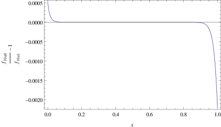
Figure 4: The inhomogeneous solution of Eq. (2) as a function of $x$. Left panel: Red dashed line: expansion around $x=0$; blue line: expansion around $x=1$. Right panel: illustration of the relative accuracy and overlap of the two solutions $f_{8a}(x)$ around 0 and 1.

Figure 5: The inhomogeneous solution of Eq. (2) as a function of $x$. Left panel: Red dashed line: expansion around $x=0$; blue line: expansion around $x=1$. Right panel: illustration of the relative accuracy and overlap of the two solutions $f_{9a}(x)$ around 0 and 1.

Figure 6: The inhomogeneous solution of Eq. (2.34) as a function of $x$. Left panel: Red dashed line: expansion around $x=0$; blue line: expansion around $x=1$. Right panel: illustration of the relative accuracy and overlap of the two solutions $f_{10a}(x)$ around 0 and 1.

at $x=0,1$ and a very similar behaviour for the approximation around $x=0$ and 1 as in the case of $f_{8a}$. Figure 6 shows the function $f_{10a}$, for which the boundaries are

$$f_{10a}(0)=-\frac{19}{72}\pi^{4}+\frac{2}{3}\pi^{2}\psi^{(1)}\left(\frac{1}{3}\right)-\psi^{(1)}\left(\frac{1}{3}\right)^{2}+6\zeta_{3}\leavevmode\nobreak\ \leavevmode\nobreak\ \leavevmode\nobreak\ \leavevmode\nobreak\ \leavevmode\nobreak\ \text{and}\leavevmode\nobreak\ \leavevmode\nobreak\ \leavevmode\nobreak\ \leavevmode\nobreak\ \leavevmode\nobreak\ f_{10a}(1)=2{\sf B}_{4}-9\zeta_{4}\leavevmode\nobreak\ .$$ (5.31)

Here somewhat larger deviations of the series solutions around $x=0$ at 1 and $x=1$ at 0 are visible.

Figure 7: The inhomogeneous solution of Eq. (2.32) as a function of $x$. Left panel: Red dashed line: expansion around $x=0$; blue line: expansion around $x=1$. Right panel: illustration of the relative accuracy and overlap of the two solutions $f_{8b}(x)$ around 0 and 1.

In Figure 7 the behaviour of $f_{8b}(x)$ is illustrated. The series expansion around $x=0$ starts to diverge at $x\sim 0.4$, while the expansion around $x=1$ still holds at $x\sim 0.1$. The boundary values of $f_{8b}$ at $x=0,1$ are

$$f_{8b}(0)=-\frac{145}{48}-\frac{1}{2}\zeta_{2}\leavevmode\nobreak\ \leavevmode\nobreak\ \leavevmode\nobreak\ \leavevmode\nobreak\ \leavevmode\nobreak\ \text{and}\leavevmode\nobreak\ \leavevmode\nobreak\ \leavevmode\nobreak\ \leavevmode\nobreak\ \leavevmode\nobreak\ f_{8b}(1)=\frac{275}{12}\leavevmode\nobreak\ .$$ (5.32)

There is a numerical artefact in Figure 7b at $x\sim 0.14$ implied by the zero-transition of $f_{8b}$ in this region.

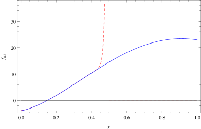
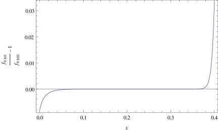
Figure 8: The inhomogeneous solution of Eq. (2.33) as a function of $x$. Left panel: Red dashed line: expansion around $x=0$; blue line: expansion around $x=1$. Right panel: illustration of the relative accuracy and overlap of the two solutions $f_{9b}(x)$ around 0 and 1.

A similar behaviour to that of $f_{8b}$ is exhibited by $f_{9b}(x)$, shown in Figure 8. Again the series-solution around $x=0$ starts to diverge for $x\sim 0.4$. However, the one around $x=1$ holds even below $x\sim 0.1$. The boundary values of $f_{9b}$ at $x=0,1$ are

$$f_{9b}(0)=\frac{25}{6}+\zeta_{2}\leavevmode\nobreak\ \leavevmode\nobreak\ \leavevmode\nobreak\ \leavevmode\nobreak\ \leavevmode\nobreak\ \text{and}\leavevmode\nobreak\ \leavevmode\nobreak\ \leavevmode\nobreak\ \leavevmode\nobreak\ \leavevmode\nobreak\ f_{9b}(1)=\frac{5}{3}\leavevmode\nobreak\ .$$ (5.33)

$f_{10b}(x)$ is shown in Figure 9. The validity of the serial expansions around $x=0$ and 1 are very similar to the cases of $f_{8(9)b}(x)$, discussed above.

Figure 9: The inhomogeneous solution of Eq. (2.35) as a function of $x$. Left panel: Red dashed line: expansion around $x=0$; blue line: expansion around $x=1$. Right panel: illustration of the relative accuracy and overlap of the two solutions $f_{10b}(x)$ around 0 and 1.

The boundary values at $x=0,1$ are

$$f_{10b}(0)=3\zeta_{4}+6\zeta_{3}\leavevmode\nobreak\ \leavevmode\nobreak\ \leavevmode\nobreak\ \leavevmode\nobreak\ \leavevmode\nobreak\ \text{and}\leavevmode\nobreak\ \leavevmode\nobreak\ \leavevmode\nobreak\ \leavevmode\nobreak\ \leavevmode\nobreak\ f_{10b}(1)=2{\sf B}_{4}-9\zeta_{4}\leavevmode\nobreak\ .$$ (5.34)

Notice that the representations (2.32, 5.2) allow for the analytic determination of the $N$th expansion coefficient of the corresponding series around $x=0\leavevmode\nobreak\ (y=0)$ using the techniques of the package HarmonicSums.m [HARMONICSUMS, Ablinger:PhDThesis, Ablinger:2011te, Ablinger:2013cf, Ablinger:2014bra].

The series expansions agree with those obtained by solving the differential equations through series Ansätze in [Grigo:2012ji]. In an attachment to this paper, we present the expansion of the solutions around $x=0$ and $x=1$ up to terms of $O(x^{50})$ for further use. The solutions are well overlapping in wider ranges in $x$. In the case of the functions $f_{8(9,10)a}(x)$ the power series expansion around $x=1$ reflects the branch point at $x=1/3$ in the homogeneous solution. Our general expressions easily allow expansions around other fixed values of $x$, which may be useful in special numerical applications.

The above representations constitute a practical analytic solution in the case of iterative non-iterative integrals. Indeed it applies to the whole class of these functions within their analyticity regions. Thus the method is not limited to cases in which elliptic integrals contribute. Since, however, the case in which ${}_{2}F_{1}$ solutions may be related in a non-trivial manner, see ii) and iii) in Section 6, to solutions through elliptic integrals with rational argument is very frequent, we turn now to a more detailed discussion of this case.

6 Elliptic Solutions

As we have seen, in special cases the solutions of a second order differential equation having a ${}_{2}F_{1}$ solution may be expressed in terms of the complete elliptic integrals ${\bf E}(r(z))$ and ${\bf K}(r(z))$. Our general goal is to represent the emerging structures in terms of $q$-series with explicit predicted expansion coefficients in closed form as far as possible, if not even simpler representations can be found.

Different levels of complexity can be distinguished, depending on the structure of $r(z)$ and whether only elliptic integrals of the first kind or also of the second kind necessarily contribute. Furthermore, there are requirements to other building blocks emerging in the solutions, which we will discuss below.

1. If the complete elliptic integrals are given by ${\bf K}(z)$ or ${\bf K}(1-z)$, choosing the case $z\in[0,1]$, and similarly for ${\bf E}$, one may solve the difference equation, obtained from the differential equation by a Mellin transform. It turns out that this difference equation factorizes to first order, unlike the differential equation in $x$-space; see [vonManteuffel:2017hms] for an example. The Mellin transforms (1.1) are given by

   $${\rm\bf M}[{\bf K}(1-z)](N) = \frac{2^{4N+1}}{\displaystyle(1+2N)^{2}\binom{2N}{N}^{2}}$$ (6.1)

   $${\rm\bf M}[{\bf E}(1-z)](N) = \frac{2^{4N+2}}{\displaystyle(1+2N)^{2}(3+2N)\binom{2N}{N}^{2}},$$ (6.2)

   since

   $${\bf K}(1-z) = \frac{1}{2}\frac{1}{\sqrt{1-z}}\otimes\frac{1}{\sqrt{1-z}}$$ (6.3)

   $${\bf E}(1-z) = \frac{1}{2}\frac{z}{\sqrt{1-z}}\otimes\frac{1}{\sqrt{1-z}}\leavevmode\nobreak\ .$$ (6.4)

   Here the Mellin convolution is defined by

   $$A(z)\otimes B(z) = \int_{0}^{1}dz_{1}\int_{0}^{1}dz_{2}\delta(z-z_{1}z_{2})A(z_{1})B(z_{2}).$$ (6.5)

   Eqs. (6.1) and (6.2) are hypergeometric terms in $N$, which has been shown already in Ref. [Ablinger:2013eba] for ${\bf K}(1-z)$, see also [Ablinger:2014bra]. As we outlined in Ref. [Ablinger:2015tua] the solution of systems of differential equations or difference equations can always be obtained algorithmically in the case either of those factorizes to first order. The transition to $z$-space is then straightforward. In $z$-space also the analytic continuation to the other kinematic regions is performed.

2. In a second set of cases, only the elliptic integrals ${\bf K}(r(z))$ and ${\bf K}^{\prime}(r(z))$ contribute, with $r(z)$ a rational function. In transforming from $z$- to $q$-space, furthermore, no terms in the solution emerge which cannot be expressed in terms of modular forms [KF, KOECHER, MILNE, RADEMACHER, DIAMOND, SCHOENENBERG, APOSTOL, KOEHLER, ONO, MIYAKE, SERRE, MART1], except terms $\propto\ln^{k}(q),k\leavevmode\nobreak\ \in\leavevmode\nobreak\ \mathbb{N}$. This is the situation e.g. in Refs. [BLOCH2, Adams:2014vja, Adams:2016xah]. We will show below that here both the homogenous solution and the integrand of the inhomogeneous solution can be expressed by Lambert–Eisenstein series [LAMBERT, EISENSTEIN], also known as elliptic polylogarithms, modulo eventual terms $\ln^{k}(q)$. The remaining $q$-integral in the inhomogeneous term can be carried out in the class of elliptic polylogarithms [ELLPOL], see [Adams:2016xah].

3. In the cases presented in Section 3, the solutions depend both on the elliptic integrals ${\bf K}(r(z))$, ${\bf E}(r(z))$ and ${\bf K}^{\prime}(r(z))$, ${\bf E}^{\prime}(r(z))$, see also Section LABEL:sec:6.2. Both ${\bf E}(r(z))$ and ${\bf E}^{\prime}(r(z))$ can be mapped to modular forms representing them by the nome $q$ according to Eqs. (1.2, 1.3), powers of $\ln(q)$, and polylogarithms, like ${\rm Li}_{0}(q)$ [GH], and the $\eta$-factor given in Eq. (1.4). These aspects lead to a generalization w.r.t. the cases covered by ii), since in a series of building blocks the factor $1/\eta^{k}(\tau)$ has to be split off to obtain a suitable modular form. This factor is a $q$-Pochhammer symbol and also emerges in the $q$-integral in the inhomogeneous solution.

Since the topic of analytic $q$-series representations is a very recent one and it is only on the way to be algorithmized and automated for the application to a larger number of cases appearing in Feynman parameter integrals, we are going to summarize the necessary definitions and central properties for a wider audience in Section 6.1. Then we will show in Section LABEL:sec:6.2 that in the case of the differential equations (2, 2.32) both the elliptic integrals K and E are contributing, which implies the appearance of the additional $\eta$-factor (1.4). In Section LABEL:sec-52 we will then construct the building blocks for the homogeneous and inhomogeneous solutions of all terms through polynomials of $\eta$-weighted Lambert–Eisenstein series, referring to the examples (3.18, 3.19). Here we use methods of the theory of modular functions and modular forms.

6.1 From Elliptic Integrals to Lambert–Eisenstein Series

There are various sets of functions which can be used to express the complete elliptic integrals and their inverse, the elliptic functions, which have been worked out starting with Euler [EUL3], Legendre [LEGENDRE] and Abel [ABEL], followed by Jacobi’s seminal work [JAC1, JAC2] and the final generalization by Weierstraß [WEIER]. We first present a collection of relations out of the theory of elliptic integrals, their related functions and modular forms [KF, KOECHER, MILNE] for the convenience of the reader. They are essential to derive integrals over complete elliptic integrals at rational arguments, which can be represented in terms of elliptic polylogarithms. Later, we will consider the different steps for a representation of the inhomogeneous solution based on the homogeneous solutions $\psi_{3}$ and $\psi_{4}$ given before.

We first summarize a series of properties of Jacobi $\vartheta_{i}$ and the Dedekind $\eta$ functions in Section 6.1.1, followed by the representation of the complete elliptic integrals of the first and second kind by the parameters of the elliptic curve and by the Jacobi $\vartheta_{i}$ and the Dedekind $\eta$ functions in Section 6.1.2. Basic facts about modular functions and modular forms are summarized in Section 6.1.3 for the later representation of the building blocks of the homogeneous and inhomogeneous solutions of the second order differential equations of Section 2. In Section LABEL:sec:6.1.5 we collect some relations on elliptic polylogarithms and give representations of $\eta$-ratios in terms of modular forms weighted by a factor $1/\eta^{k}(\tau)$ in Section LABEL:sec:6.1.4. The modular forms are expressed over bases formed by Lambert–Eisenstein series and products thereof.

6.1.1 The Jacobi $\vartheta_{i}$ and Dedekind $\eta$ Functions

As entrance point we use Jacobi’s $\vartheta_{i}$ functions [JAC2]. The $\vartheta$ functions possess $q$-series and product representations

$$\vartheta_{1}(q,z) = \sum_{k=-\infty}^{\infty}(-1)^{\left(k-\tfrac{1}{2}\right)}q^{(k+1/2)^{2}}\exp[(2k+1)iz]=2q^{\tfrac{1}{4}}\sum_{k=0}^{\infty}(-1)^{n}q^{n(n+1)}\sin[(2n+1)z]$$

$$\vartheta_{2}(q,0) \equiv \vartheta_{2}(q)=\sum_{k=-\infty}^{\infty}q^{(k-1/2)^{2}}$$ (6.7)

$$\vartheta_{3}(q,0) \equiv \vartheta_{3}(q)=\sum_{k=-\infty}^{\infty}q^{k^{2}}$$ (6.8)

$$\vartheta_{4}(q,0) \equiv \vartheta_{4}(q)=\sum_{k=-\infty}^{\infty}(-1)^{k}q^{k^{2}}.$$ (6.9)

The elliptic polylogarithms, introduced in (LABEL:eq:ELP1, LABEL:eq:ELP2) below are also $q$-series, containing a specific parameter pattern which allows to accommodate certain classes of $q$-series emerging in Feynman integral calculations. The product representations associated to (6.7–6.9) read

$$\vartheta_{2}(q) = 2q^{\frac{1}{4}}\prod_{k=1}^{\infty}\left(1-q^{2k}\right)\left(1+q^{2k}\right)^{2}$$ (6.10)

$$\vartheta_{3}(q) = \prod_{k=1}^{\infty}\left(1-q^{2k}\right)\left(1+q^{2k-1}\right)^{2}$$ (6.11)

$$\vartheta_{4}(q) = \prod_{k=1}^{\infty}\left(1-q^{2k}\right)\left(1-q^{2k-1}\right)^{2}.$$ (6.12)

They are closely related to Euler’s totient function [EUL4]

$$\phi(q)=\prod_{k=1}^{\infty}\frac{1}{1-q^{k}},$$ (6.13)

the first emergence of $q$-products, and to Dedekind’s $\eta$ function [DEDEKINDeta].

$$\eta(\tau)=\frac{q^{\frac{1}{12}}}{\phi(q^{2})}.$$ (6.14)

One has

$$\vartheta_{2}(q) = \frac{2\eta^{2}(2\tau)}{\eta(\tau)}$$ (6.15)

$$\vartheta_{3}(q) = \frac{\eta^{5}(\tau)}{\eta^{2}\left(\frac{1}{2}\tau\right)\eta^{2}(2\tau)}$$ (6.16)

$$\vartheta_{4}(q) = \frac{\eta^{2}\left(\frac{1}{2}\tau\right)}{\eta(\tau)}.$$ (6.17)

In the following we will make use of series representations of both Jacobi $\vartheta$- and Dedekind $\eta$-functions. We list a series of important relations for convenience :

$$\eta(\tau+n) =e^{i\frac{\pi n}{12}}\eta(\tau),\leavevmode\nobreak\ \leavevmode\nobreak\ \leavevmode\nobreak\ n\in\mathbb{N}$$ (6.18)

$$\eta(\tau) =q^{\frac{1}{12}}\sum_{k=-\infty}^{\infty}(-1)^{k}q^{3k^{2}+k}$$ [EULER1] (6.19)

$$\eta^{3}(\tau) =q^{\frac{1}{4}}\sum_{k=-\infty}^{\infty}(4k+1)q^{4k^{2}+2k}$$ [JAC1] (6.20)

$$\frac{\eta^{2}(\tau)}{\eta(2\tau)} =\sum_{k=-\infty}^{\infty}(-1)^{k}q^{2k^{2}}$$ [GAUSS2] (6.21)

$$\frac{\eta^{2}(2\tau)}{\eta(\tau)} =q^{\frac{1}{4}}\sum_{k=-\infty}^{\infty}q^{4k^{2}+2k}$$ [GAUSS2] (6.22)

$$\frac{\eta(2\tau)^{5}}{\eta(\tau)^{2}} =q^{\frac{2}{3}}\sum_{k=-\infty}^{\infty}(-1)^{k}(3k+1)q^{6k^{2}+4k}$$ [GORDON1] (6.23)

$$\frac{\eta(\tau)^{5}}{\eta(2\tau)^{2}} =q^{\frac{1}{12}}\sum_{k=-\infty}^{\infty}(6k+1)q^{3k^{2}+k}$$ [GORDON1] (6.24)

$$\frac{\eta(\tau)\eta(6\tau)^{2}}{\eta(2\tau)\eta(3\tau)} =q^{\frac{2}{3}}\sum_{k=-\infty}^{\infty}(-1)^{k}q^{6k^{2}+4k}$$ [KAC] (6.25)

$$\frac{\eta(2\tau)\eta(3\tau)^{2}}{\eta(\tau)\eta(6\tau)} =q^{\frac{1}{12}}\sum_{k=-\infty}^{\infty}q^{3k^{2}+k}$$ [KAC] (6.26)

$$\frac{\eta(\tau)^{2}\eta(6\tau)}{\eta(2\tau)\eta(3\tau)} =q^{\frac{1}{4}}\sum_{k=-\infty}^{\infty}\left(q^{9k^{2}+3k}-q^{(3k+1)(3k+2)}\right).$$ [KAC] (6.27)

Many other identities hold and can be found e.g. in Refs. [KOEHLER, MACDONALD, KAC, LEPOWSKY, ZUCKER, MARTIN, WILLIAMS, KENDRIL, ONO].

6.1.2 Representations of the Modulus and the Elliptic Integrals

For later use we consider also the structure of the differential equation of the Weierstraß’ function $\wp(z)$ [WEIER],

$$\wp^{\prime 2}(z)=4\wp^{3}(z)-g_{2}\wp(z)-g_{3}=4(\wp(z)-e_{1})(\wp(z)-e_{2})(\wp(z)-e_{3})\leavevmode\nobreak\ .$$ (6.28)

The functions $g_{2},g_{3},e_{1},e_{2}$ and $e_{3}$ are given by

$$g_{2} = -4[e_{2}e_{3}+e_{3}e_{1}+e_{1}e_{2}]=2[e_{1}^{2}+e_{2}^{2}+e_{3}^{2}]$$ (6.29)

$$g_{3} = 4e_{1}e_{2}e_{3}=\frac{4}{3}[e_{1}^{3}+e_{2}^{3}+e_{3}^{3}]$$ (6.30)

$$e_{1}+e_{2}+e_{3} = 0,$$ (6.31)

Figure 10: The elliptic curve for $k=0$ (dashed blue line), $k=1/2$ (dotted black lines), and $k=1/\sqrt{2}$ full red lines.

and the following representation in terms of Jacobi $\vartheta$ functions holds:

$$e_{1} = \leavevmode\nobreak\ \leavevmode\nobreak\ \frac{\pi^{2}}{12\omega^{2}}\left[\vartheta_{3}^{4}(q)+\vartheta_{4}^{4}(q)\right]$$ (6.32)

$$e_{2} = \leavevmode\nobreak\ \leavevmode\nobreak\ \frac{\pi^{2}}{12\omega^{2}}\left[\vartheta_{2}^{4}(q)+\vartheta_{4}^{4}(q)\right]$$ (6.33)

$$e_{3} = -\frac{\pi^{2}}{12\omega^{2}}\left[\vartheta_{2}^{4}(q)+\vartheta_{3}^{4}(q)\right].$$ (6.34)

Here Jacobi’s identity is implied by (6.31) with

$$\vartheta_{3}^{4}(q) = \vartheta_{2}^{4}(q)+\vartheta_{4}^{4}(q)\leavevmode\nobreak\ .$$ (6.35)

The r.h.s. of (6.28) parameterizes the elliptic curve

$$y^{2}=4(x-e_{1})(x-e_{2})(x-e_{3})$$ (6.36)

of the corresponding problem. Setting $e_{1}-e_{2}=1$ for the purpose of illustration, the elliptic curves corresponding to the module $k$ is shown in Figure 10, choosing specific values.

The modulus $k$ can be represented in terms of the functions $e_{i}$ by

$$k^{2}=z(x),$$ (6.37)

cf. (3.8, 3.20). $k$ and $k^{\prime}=\sqrt{1-k^{2}}$ are given by

$$k = \sqrt{\frac{e_{3}-e_{2}}{e_{1}-e_{2}}}=\frac{\vartheta_{2}^{2}(q)}{\vartheta_{3}^{2}(q)}\equiv\frac{4\eta^{8}(2\tau)\eta^{4}\left(\frac{\tau}{2}\right)}{\eta^{12}(\tau)}$$ (6.38)

$$k^{\prime} = \sqrt{\frac{e_{1}-e_{3}}{e_{1}-e_{2}}}=\frac{\vartheta_{4}^{2}(q)}{\vartheta_{3}^{2}(q)}\equiv\frac{\eta^{4}(2\tau)\eta^{8}\left(\frac{\tau}{2}\right)}{\eta^{12}(\tau)},$$ (6.39)

cf. (6.28), which implies the following relation for $\eta$ functions

$$1=\frac{\eta^{8}\left(\frac{\tau}{2}\right)\eta^{8}(2\tau)}{\eta^{24}(\tau)}\left[16\eta^{8}(2\tau)+\eta^{8}\left(\frac{\tau}{2}\right)\right]\leavevmode\nobreak\ .$$ (6.40)

Further, one may express the elliptic integral of the first kind K by

$${\bf K}(k^{2}) = \omega\sqrt{e_{1}-e_{3}},\leavevmode\nobreak\ \leavevmode\nobreak\ \leavevmode\nobreak\ \leavevmode\nobreak\ \text{with}\leavevmode\nobreak\ \leavevmode\nobreak\ \leavevmode\nobreak\ \leavevmode\nobreak\ \sqrt{e_{1}-e_{3}}=\frac{\pi}{2\omega}\vartheta_{3}^{2}(q)\equiv\frac{\pi}{2}\frac{\eta^{10}(\tau)}{\eta^{4}\left(\frac{\tau}{2}\right)\eta^{4}(2\tau)},$$ (6.41)

$${\bf K^{\prime}}(k^{2}) = -\frac{1}{\pi}{\bf K}(k^{2})\leavevmode\nobreak\ \ln(q)\leavevmode\nobreak\ .$$ (6.42)

Sometimes one also introduces the Jacobi functions $\omega,\omega^{\prime},\eta$ and $\eta^{\prime}$, which are defined by

$$\omega = \frac{{\bf K}}{\sqrt{e_{1}-e_{3}}}$$ (6.43)

$$\omega^{\prime} = i\frac{{\bf K^{\prime}}}{\sqrt{e_{1}-e_{3}}}=\omega\tau=\frac{\omega}{i\pi}\ln(q)$$ (6.44)

$$\eta = -\frac{1}{12\omega}\frac{\vartheta_{1}^{\prime\prime\prime}(q)}{\vartheta_{1}^{\prime}(q)},$$ (6.45)

with

$$\vartheta_{1}^{(k)}(q)=\lim_{z\rightarrow 0}\frac{d^{k}}{dz^{k}}\vartheta_{1}(q,z).$$ (6.46)

The function $\eta^{\prime}$ can be obtained using Legendre’s identity (3.21) in the form

$$\eta\omega^{\prime}-\eta^{\prime}\omega=i\frac{\pi}{2}.$$ (6.47)

One obtains the following representations of the elliptic integrals of the second kind by

$${\bf E}(k^{2}) = \frac{e_{1}\omega+\eta}{\sqrt{e_{1}-e_{3}}}$$ (6.48)

$${\bf E^{\prime}}(k^{2}) = i\frac{e_{3}\omega^{\prime}+\eta^{\prime}}{\sqrt{e_{1}-e_{3}}}.$$ (6.49)

Later on we will use the relation [ERDELYI2, ABRSTE] for E

$${\bf E}(k^{2}) = {\bf K}(k^{2})+\frac{\pi^{2}q}{{\bf K}(k^{2})}\frac{d}{dq}\ln\left[\vartheta_{4}(q)\right]$$ (6.50)

and the Legendre identity (3.21) to express E^′,

$${\bf E}^{\prime}(k^{2}) = \frac{\pi}{2{\bf K}(k^{2})}\left[1+2\ln(q)\leavevmode\nobreak\ q\frac{d}{dq}\ln\left[\vartheta_{4}(q)\right]\right].$$ (6.51)

6.1.3 Modular Forms and Modular Functions

All building blocks forming the homogeneous solutions and the integrand of the inhomogeneous solutions of the second order differential equations considered above can be expressed in terms of $\eta$-ratios. They are defined as follows.

Definition 6.1.

Let $r=\left(r_{\delta}\right)_{\delta|N}$ be a finite sequence of integers indexed by the divisors $\delta$ of $N\in\mathbb{N}\backslash\{0\}$. The function $f_{r}(\tau)$

$$f_{r}(\tau):=\prod_{d|N}\eta(d\tau)^{r_{d}},\leavevmode\nobreak\ \leavevmode\nobreak\ \leavevmode\nobreak\ d,N\in\mathbb{N}\backslash\{0\},\leavevmode\nobreak\ \leavevmode\nobreak\ r_{d}\in\mathbb{Z},$$ (6.52)

is called $\eta$-ratio.

These are modular functions or modular forms; the former ones can be obtained as the ratio of two modular forms. In the following we summarize a series of basic facts on these quantities in a series of definitions and theorems needed in the calculation of the present paper, cf. also Refs. [KF, KOECHER, MILNE, RADEMACHER, DIAMOND, SCHOENENBERG, APOSTOL, KOEHLER, ONO, MIYAKE, SERRE, MART1].