Dynamic Anisotropy in MHD Turbulence induced by mean magnetic field

Abstract

In this paper we study the development of anisotropy in strong MHD turbulence in the presence of a large scale magnetic field $B_{0}$ by analyzing the results of direct numerical simulations. Our results show that the developed anisotropy among the different components of the velocity and magnetic field is a direct outcome of the inverse cascade of energy of the perpendicular velocity components $\bf u_{\perp}$ and a forward cascade of the energy of the parallel component $\bf u_{\parallel}$. The inverse cascade develops for strong ${B_{0}}$ where the flow exhibits strong vortical structure by the suppression of fluctuations along the magnetic field. Both the inverse and the forward cascade are examined in detail by investigating the anisotropic energy spectra, the energy fluxes and the shell to shell energy transfers among different scales.

I Introduction

Magnetohydrodynamics (MHD) provides the macroscopic equations for the motion of a conducting fluid that is coupled with the electrodynamics equations. MHD flows are ubiquitous in nature, and they are observed in the interstellar medium, galaxies, accretion disks, star and planet interiors, solar wind, Tokamak etc. In such flows, the kinetic Reynolds number $Re$ (defined as $Re=UL/\nu$, where $U$ is the rms velocity, $L$ is the domain size, and $\nu$ is the kinematic viscosity) and magnetic Reynolds number $Rm$ (defined as $Rm=UL/\eta$, where $\eta$ is the magnetic diffusivity) are so large that the flows are turbulent with a large continuous range of excited scales, from the largest scales where energy is injected to the smallest scales where energy is dissipated. Furthermore, in most of these systems, reasonably strong magnetic fields are known to exist, with correlation lengths much larger than those of the turbulent flow. These large-scale magnetic fields present in these systems induce dynamic anisotropy, and hence play significant dynamical role in the flow evolution.

Resolving both the large scale magnetic fields and the small scale turbulence by direct numerical simulations is still a major challenge even with the presently available supercomputers (see Alexakis (2013)). One of the possible simplifications around this difficulty is to model the large-scale magnetic field by a uniform magnetic field ${B_{0}}$, and study its effect on the small scale turbulence. This approximation simplifies the analysis of the system as it allows to study the effect of large magnetic fields on small scale turbulence without tracking down their slow evolution. For example, various features of the solar corona (e.g., the magnetic structures associated with prominence, coronal holes with their open field lines, and coronal loops) are modeled using such a “magnetofluid with mean ${B_{0}}$ field” approximation. Other systems of interest where such an approximation is advantageous include the solar wind, where the inertial-range fluctuations are subjected to a mean magnetic field, and fusion devices, like ITER, that involve large toroidal magnetic fields.

MHD turbulence in the presence of a mean magnetic field has been the subject of many studies  (Iroshnikov, 1963; Kraichnan, 1965; Shebalin et al., 1983; Zank and Matthaeus, 1993; Oughton et al., 1994). The initial phenomenological estimates for the energy spectrum $E(k)$ based on Alfvén effects and isotropy lead to the prediction of an energy spectrum $E(k)\propto k^{-3/2}$ Iroshnikov (1963); Kraichnan (1965). Verma Verma (1999, 2004) showed that the “random” large-scale mean magnetic field ${B_{0}}$ gets renormalized to yield $B_{0}(k)\sim k^{-1/3}$ and Kolmogorov-like energy spectrum ($E(k)\sim k^{-5/3}$). This result is also consistent with energy spectrum derived by re-normalizing viscosity and resistivity Verma (2001).

The presence of a large-scale mean magnetic field however supports propagation of Alfvén waves that makes the flow anisotropic. The first studies of anisotropy by Shebalin et. al. Shebalin et al. (1983) in two-dimensional magnetohydrodynamics and by Oughton et al. Oughton et al. (1994) in three dimensions quantified the anisotropy by measuring the angles

$$\theta_{u,b}=\tan^{-1}\frac{\sum_{k}k_{z}^{2}E_{u,b}({\bf k})}{\sum_{k}(k_{x}^{2}+k_{y}^{2})E_{u,b}({\bf k})}.$$ (1)

where $E_{u,b}$ is the velocity or magnetic field energy spectrum, and $\hat{z}$ is the direction of the mean magnetic field. In their low-resolution simulations ($k_{\mathrm{max}}=32$), they employed ${B_{0}}=0$ to $16$, and showed that strong anisotropy arises due to the mean magnetic field with the anisotropy being strongest at higher wavenumbers and thus it can not be neglected. Phenomenological theories that take in to account anisotropy predict that the anisotropic energy spectrum scales as $k_{\perp}^{-5/3}$ Goldreich and Sridhar (1995) (where $k_{\perp}$ is the wave number perpendicular to the mean magnetic field) or as $k_{\perp}^{-3/2}$ Boldyrev (2006). Simulations of Boldyrev et al. Boldyrev and Perez (2009); Perez et al. (2012, 2014) support $-3/2$ exponent, while those by Beresnyak Beresnyak and A. (2009); Beresnyak (2011, 2014) argue in favour of Kolmogorov’s exponent $-5/3$. Thus, at present there is no consensus on the energy spectrum for the MHD turbulence.

The only case that analytical results have been derived is the weak turbulence limit where the uniform magnetic field is assumed to be very strong. In this limit, the evolution of the energy spectrum can be calculated analytically using an asymptotic expansion (Galtier et al., 2000) that leads to the prediction $E(k_{\perp})\propto k_{\perp}^{-2}$. The predictions above however are valid only in large enough domains in which many large-scale modes along the mean magnetic field exist. In finite domains one finds an even richer behavior. It has been shown (Alexakis, 2011; Reddy and Verma, 2014; Reddy et al., 2014) with the use of numerical simulations that in finite domains, three-dimensional MHD flows become quasi-two-dimensional for strong external magnetic field. These states exhibit high anisotropy with very weak variations along the direction of the magnetic field and resembles two-dimensional turbulence. In fact, it can be shown that for ${B_{0}}$ above a critical value, the aforementioned two-dimensionalisation becomes exact Gallet and Doering (2015), with three-dimensional perturbations dying off exponentially in time. At intermediate values of ${B_{0}}$, however, three-dimensional perturbations are present and control the forward cascade of energy.

The degree of anisotropy in such quasi two-dimensionalized situations has been studied more recently. To quantify scale-by-scale anisotropy, Alexakis et al. Alexakis et al. (2007); Alexakis (2011) partitioned the wavenumber space into coaxial cylindrical domains aligned along the mean magnetic field direction, and into planar domains transverse to mean field. Using this decomposition, Alexakis Alexakis (2011) studied the energy spectra and fluxes, as well as two-dimensionalization of the flow for mean magnetic field strengths ${B_{0}}=2$, $5$, and $10$. He reported an inverse energy cascade for the wavenumbers smaller than the forcing wavenumbers. Teaca et al. Teaca et al. (2009) decomposed the spectral space into rings, and arrived at similar conclusion as above. Teaca et al. observed that the energy tends to concentrate near the equator strongly as the strength of the magnetic field is increased. They also showed that the constant magnetic field facilitates energy transfers from the velocity field to the magnetic field. In the present paper, we study in detail the development of anisotropy in such flows and relate it to the development of the inverse cascade.

The outline of the paper is as follows. We introduce the theoretical framework in Sec. II followed by details of the numerical simulations in Sec. III. Next, we discuss the anisotropic spectra in Sec. IV, and energy transfers diagnostics like energy flux and shell-to-shell energy transfers in Sec. V. Finally, we conclude in section VI.

II Setup and governing equations

We consider an incompressible flow of a conducting fluid in the presence of a constant and strong guiding magnetic field ${\bf B_{0}}$ along $\hat{z}$ direction. The incompressible MHD equations (Roberts, 1967; Verma, 2004) are given below:

$$\frac{\partial}{\partial t}{\bf u}+({\bf u}\cdot\nabla)\mathbf{u}=-\nabla P+({\bf B}\cdot\nabla)\mathbf{b}+\nu{\nabla}^{2}\mathbf{u}+\mathbf{f}$$

$$\frac{\partial}{\partial t}{\bf b}+({\bf u}\cdot\nabla)\mathbf{b}=({\bf B}\cdot\nabla)\mathbf{u}+\eta\nabla^{2}\mathbf{b}$$ (2)

$$\nabla\cdot\mathbf{u}=0,\qquad\nabla\cdot\mathbf{b}=0.$$

Here ${\bf u}$ is the velocity field, ${\bf B}$ is the magnetic field, ${\bf f}$ is the external forcing, $P$ is the total (thermal + magnetic) pressure, $\nu$ is the viscosity, and $\eta$ is the magnetic diffusivity of the fluid. We take $\nu=\eta$, thus the magnetic Prandtl number $Pm=\nu/\eta$ is unity. The total magnetic field is decomposed into its mean part ${B_{0}}\hat{z}$ and the fluctuating part ${\bf b}$, i.e. ${\bf B}={B_{0}}\hat{z}+{\bf b}$. Note that in the above equations, the magnetic field has the same units as the velocity field.

The above equations were solved using a parallel pseudospectral parallel code Ghost Mininni et al. (2011) with a grid resolution $512^{3}$ and a fourth order Runge-Kutta method for time stepping. The simulation box is of the size $(2\pi)^{3}$ on which periodic boundary condition on all directions were employed. The velocity field was forced randomly at the intermediate wavenumbers satisfying $8\leq|k|\leq 10$. This allowed to observe the development of both the inverse cascade and the forward cascade when they are present. The simulations were evolved for sufficiently long times so that either a steady state was reached, or until we observe dominant energy at the largest scales due to the inverse cascade of energy (for large ${B_{0}}$). In the simulations the forcing amplitude was controlled, while the saturation level of the kinetic energy is a function of the other control parameters of the system. Thus, the more relevant non-dimensional control parameter is the Grasshof number defined as $G\equiv\|{\bf f}\|L^{3}/\nu^{2}$, where $\|\cdot\|$ stands for the $L_{2}$ norm, and $L=2\pi$ is the length scale of the system. Alternatively, we can use the Reynolds number $Re=\|{\bf u}\|L/\nu$ based on the rms value of the velocity. Note however that $Re$ evolves in time in the presence of an inverse cascade. For further details of simulations, refer to Alexakis Alexakis (2011).

We examine two different values of ${B_{0}=2}$ and $10$. The results of these simulations were first presented in Alexakis (2011) and correspond to the runs R2 and R3 respectively in that work. The values of the control parameters used and of the basic observable are summarized in table 1. The runs have relatively moderate Reynolds number due to the forcing at intermediate wavenumbers. Therefore we do not focus on the energy spectra. Rather we aim to unravel the mechanisms that lead to the redistribution of energy and development of anisotropic turbulence due to the mean magnetic field.

Table 1: Steady-state parameters of the simulation: Grasshof number $G\equiv\|{\bf f}\|L^{3}/\nu^{2}$, Reynolds number $\|{\bf u}\|L/\nu$, kinetic and magnetic energies, ${B_{0}}/\|{\bf u}\|$, $r_{A}^{-1}=\|{\bf b}\|^{2}/\|{\bf u}\|^{2}$, kinetic and magnetic dissipation rates, anisotropic parameters $A_{u}$ and $A_{b}$(see Eq. (3)). The values are obtained from single snapshots and not by time-averaging.

$Gr^{1/2}$	$Re$	${B_{0}}$	$\|{\bf u}\|^{2}$	$\|{\bf b}\|^{2}$	${B_{0}}/\|{\bf u}\|$	$r_{A}^{-1}$	$\nu\|{\bf\nabla u}\|^{2}$	$\eta\|{\bf\nabla b}\|^{2}$	$A_{u}$	$A_{b}$
2500	$1.09\times 10^{4}$	2	0.24	0.18	4.08	0.75	0.043	0.041	0.53	0.73
2500	$1.53\times 10^{4}$	10	0.47	0.012	14.6	0.026	0.015	0.0021	3.7	1.6

In later sections, we analyze the anisotropic energy spectra and energy transfer diagnostics using the generated numerical data by employing another pseudo-spectral code Tarang Verma et al. (2013). We describe the anisotropic energy spectra, as well as the fluxes and the energy transfers involving the velocity and magnetic fields, generated during the evolved state. Throughout the paper, we denote $u_{\parallel}=u_{z}$ and ${\bf u}_{\perp}=(u_{x},u_{y})$.

III Spectra and anisotropy

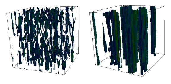
(a)                                                                                 (b)

Figure 1: Isosurfaces of magnitudes of vorticity $|\boldsymbol{\omega}|$ for mean magnetic field (a) ${B_{0}=2}$ and (b) ${B_{0}=10}$.

First we present visualizations of the two examined flows for ${B_{0}=2}$ and $10$ to demonstrate the anisotropy of the flow. In Figure 1, we present the iso-surfaces of the magnitude of the vorticity $|\boldsymbol{\omega}|$, where $\boldsymbol{\omega}=\nabla\times{\bf u}$. The flow has vortical columnar structures along ${B_{0}}$ that becomes stronger as ${B_{0}}$ is increased. To get further details of the flow structure, we make a horizontal section for the ${B_{0}=10}$ case. In Figure 2(a) we show the density plot of vorticity magnitude along with velocity vectors $(u_{x},u_{y})$. The flow develops strong vortical structure, with strong $u_{y}$ and $u_{x}$ components, while modes that vary along $\hat{z}$ are very weak. The reason for the formation of these structures is discussed in detail in Sec. IV).

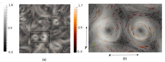
Figure 2: For ${B_{0}=10}$, a horizontal cross-sectional view of (a) density plot of $|\boldsymbol{\omega}|$ (arrows) along with the velocity vectors (gray background), The ‘grayscale’ and ‘hot-cold’ (shown by ‘dark red/brown’) colorcode correspond to the magnitude of velocity field and vorticity respectively. (b) A zoomed view of area inside black rectangle of subplot (a).

To quantify the anisotropy of the flow, we propose anisotropy measures $A_{u}$ and $A_{b}$ for the velocity and magnetic fields as

$$A_{u}=\frac{E_{u}^{\perp}}{2E_{u}^{\parallel}};~{}~{}~{}A_{b}=\frac{E_{b}^{\perp}}{2E_{b}^{\parallel}}.$$ (3)

where $E_{u}^{\perp}=\left\langle u_{x}^{2}+u_{y}^{2}\right\rangle/2$ and $E_{u}^{\parallel}=\langle u_{z}^{2}\rangle/2$, where the angular brackets stand for spatial average. The quantities $E_{u}^{\perp}$ and $E_{u}^{\parallel}$ represent the kinetic energies of the perpendicular and parallel components of the velocity field. Similar definitions are employed for the magnetic field. The anisotropy parameter $A_{u,b}$ measures the degree of anisotropy among the different components of the velocity and magnetic field. It is defined such that $A_{u,b}=1$ for isotropic flow with $\left\langle u_{x}^{2}\right\rangle=\left\langle u_{y}^{2}\right\rangle=\left\langle u_{z}^{2}\right\rangle$, but it deviates from unity for anisotropic flows. In Table 1, we list $A_{u}$ and $A_{b}$ for the two runs. For ${B_{0}}=2$, both $A_{u}$ and $A_{b}$ are smaller than unity, i.e. $E^{\perp}_{u}<2E^{\parallel}_{u}$ (due to the particular choice of forcing used), while for ${B_{0}}=10$, their magnitude is substantially higher than unity ($E_{\perp}>2E_{\parallel}$) that as we shall show later is due to the presence of an inverse cascade: the flow is quasi two-dimensional, hence it exhibits strong inverse cascade of kinetic energy leading to buildup of kinetic energy at large scales.

Further insight can be obtained by studying the distribution of energy among the different components and different modes in the Fourier space. For isotropic flows, the energies of all the modes and all components within a thin spherical shell in Fourier-space are statistically equal. Hence, sum of the energies of all the Fourier modes in a spherical shell of radius $k$ is often reported as one-dimensional energy spectrum $E(k)$. It provides information about the distribution of energy at different scales. The one-dimensional spectra for the velocity and the magnetic field are shown in Fig. 3. For the ${B_{0}}=10$ case, the kinetic energy peaks at the large scales while the magnetic fluctuations are suppressed. This is due to the presence of an inverse cascade of energy as discussed in Alexakis (2011) (further discussions in Sec. V). For ${B_{0}}=2$ the inverse cascade is reasonably weak, if at all. This is also consistent with the values of $A_{u}$ and $A_{b}$ (presented in Table I) for the two cases and is discussed in detail in Secs. IV-V. The dashed line indicates the $k^{-5/3}$ power-law scaling; our inertial range is too short to fit with this spectrum. As discussed in the introduction in this paper, our attempt is not to differentiate between the exponents $-3/2$ and $-5/3$, but rather study the effects of large $B_{0}$ on the global statistics of the flow.

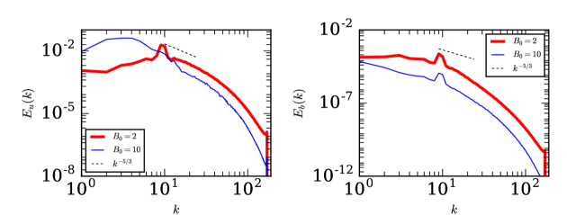
(a)                                                                  (b)

Figure 3: Plots of (a) Kinetic energy spectrum, $E_{u}(k)$ and (b) Magnetic Energy Spectrum, $E_{b}(k)$ for ${B_{0}}=2$ and $10$.

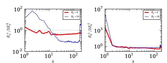
(a)                                                                  (b)

Figure 4: Plots of anisotropy spectrum of the velocity field $A_{u}(k)=\frac{E_{u}^{\perp}(k)}{2E_{u}^{\parallel}(k)}$ and magnetic field $A_{b}(k)=\frac{E_{b}^{\perp}(k)}{2E_{b}^{\parallel}(k)}$.

To explore the nature of the anisotropy at different length scales, we work in Fourier space, in which the equations are

$$\left(\frac{d}{dt}+\nu k^{2}\right){u}_{i}({\bf k})-i({\bf B}_{0}\cdot{\bf k}){b}_{i}({\bf k}) = -ik_{i}P({\bf k})-ik_{j}\sum_{{\bf k=p+q}}{u}_{j}({\bf q}){u}_{i}({\bf p})$$ (4)

$$+ik_{j}\sum_{{\bf k=p+q}}{b}_{j}({\bf q}){b}_{i}({\bf p})+{\bf f}({\bf k}),$$

$$\left(\frac{d}{dt}+\eta k^{2}\right){b}_{i}({\bf k})-i({\bf B}_{0}\cdot{\bf k}){u}_{i}({\bf k}) = -ik_{j}\sum_{{\bf k=p+q}}{u}_{j}({\bf q}){b}_{i}({\bf p})+ik_{j}\sum_{{\bf k=p+q}}{b}_{j}({\bf q}){u}_{i}({\bf p}),$$ (5)

where $\hat{\bf u}({\bf k}),\hat{\bf b}({\bf k})$ are the Fourier transform of ${\bf u,b}$ respectively. First we compute wavenumber-dependent anisotropy parameters:

$$A_{u}(k)=\frac{E_{u}^{\perp}(k)}{2E_{u}^{\parallel}(k)};~{}~{}~{}A_{b}(k)=\frac{E_{b}^{\perp}(k)}{2E_{b}^{\parallel}(k)},$$ (6)

where $E_{u}^{\perp}(k)$ represents sum of energy of the Fourier transform of ${\bf u}_{\perp}$ in the shell $(k-1:k]$. Similar definitions holds for other spectra. Fig. 4(a,b) exhibits the plots of $A_{u}(k)$ and $A_{b}(k)$ respectively. For ${B_{0}}=2$ , $A_{u}(k)>1$ for $k=1$, and $A_{u}(k)\approx 1/2$ for $k>1$. However for ${B_{0}}=10$, $A_{u}(k)$ is strongly anisotropic with $A_{u}(k)\gg 1$ for $k<k_{f}$, but $A_{u}(k)\ll 1$ for $k>k_{f}$. Thus, for ${B_{0}}=10$, the two-dimensional components in the large-scale velocity field dominate, consistent with the flow profile of Figs. 1 and 2. Note that $u_{\parallel}$ dominates over $u_{\perp}$ at large wavenumbers. This behavior is very similar to anisotropic behavior in quasi-static MHD reported by Reddy and Verma Reddy and Verma (2014) and Favier et al. Favier et al. (2010).

For magnetic field $\bf b$, $A_{b}(k)$ is very large for $k=1$, but $A_{b}(k)\sim 1$ for $1<k<k_{f}$, while it is less than unity for $k>k_{f}$. The large peak at $k=1$ for the ratio $E_{b}^{\perp}/E_{b}^{\|}$ is caused not due to excess of $E_{b}^{\perp}$ energy but rather due to the almost absence of $E_{b}^{\|}$ in the large scales. Indeed the quasi-2D motions of the flow are not able to amplify $E_{b}^{\|}$ and thus the ratio $A_{b}$ almost diverges at $k=1$. For Alfvenic turbulence where there is only a forward cascade it is observed that $|\delta B_{\perp}|^{2}\gg|\delta B_{\parallel}|^{2}$ (see  (TenBarge et al., 2012; Alexandrova et al., 2008)). However in our case as we explain later in our text part of $E_{u}^{\perp}$ and $E_{b}^{\perp}$ cascades inversely while $E_{u}^{\|}$ and $E_{b}^{\|}$ cascade forward causing an excess of $E_{b}^{\|}$ and $E_{u}^{\|}$ in the small scales.

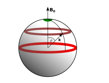
Figure 5: Illustration of the ring decomposition in the spectral space. This figure is taken from Ref. Reddy et al. (2014). [Reprinted with permission from Sandeep Reddy [K. S. Reddy, R. Kumar, and M. K. Verma, Physics of Plasmas 21, 102310 (2014). Copyright 2014, AIP Publishing].

A different measure of anisotropy is provided by looking at the distribution of energy in spectral space using a ring decomposition shown in Fig. 5 that we now discuss. A spherical shell in Fourier space is divided into rings such that each ring is characterized by two indices—the shell index $k$, and the sector index $\beta$ Teaca et al. (2009); Reddy and Verma (2014). The energy spectrum of a ring, called the ring spectrum, is defined as

$$E\left(k,\beta\right)=\frac{1}{C_{\beta}}\sum_{\begin{subarray}{c}k-1<k^{\prime}\leq k;\\ \zeta_{\beta-1}<\angle\left(\mathbf{k}^{\prime}\right)\leq\zeta_{\beta}\end{subarray}}\frac{1}{2}\left|\mathbf{\hat{u}}\left(\mathbf{k}^{\prime}\right)\right|^{2},$$ (7)

where $\angle\mathbf{k}^{\prime}$ is the angle between $\mathbf{k}^{\prime}$ and the unit vector $\hat{z}$, and the sector $\beta$ contains the modes between the angles $\zeta_{\beta-1}$ to $\zeta_{\beta}$. When $\Delta\zeta$ is uniform, the sectors near the equator contain more modes than those near the poles. Hence, to compensate for the above, we divide the sum $\sum_{k}|{\bf\hat{u}(k^{\prime})}|^{2}/2$ by the factor $C(\beta)$ given by

$$C_{\beta}=\left|\cos\left(\zeta_{\beta-1}\right)-\cos\left(\zeta_{\beta}\right)\right|.$$ (8)

For the ring spectrum computations, we divide the spectral space in the “northern” hemisphere into thin shells of unit widths (see Eq. (7)), which are further subdivided into 15 thin rings from $\theta=0$ to $\theta=\pi/2$. For the ring spectrum, we vary $k$ from 1 to $512\times(2/3)=341$; the factor 2/3 arising due to aliasing. Taking benefit of the $\theta\rightarrow(\pi-\theta)$ symmetry, we do not compute the energy of the rings in the “southern” hemisphere. In Fig. 6, we show the density plots of the kinetic and magnetic ring spectrum $E(k,\beta)$ for ${B_{0}}=2$ and $10$. From the plots it is evident that the kinetic and magnetic energy is stronger near the equator than the polar region, and the anisotropy increases with ${B_{0}}$. The anisotropy is greater for ${B_{0}}=10$, but the energy is concentrated near the equator even for ${B_{0}}=2$.

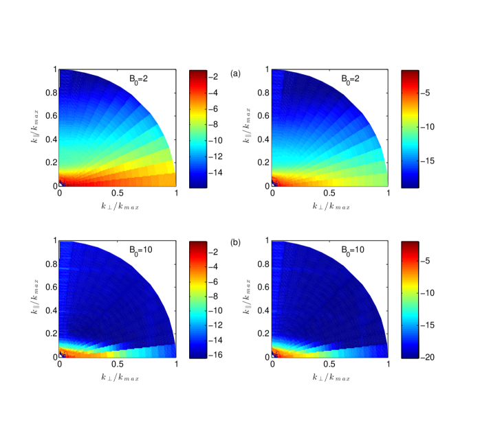
Figure 6: The ring spectra in log scale: $\log(E_{u}(k,\theta))$ (left) and $\log(E_{b}(k,\theta))$ (right) for (a)${B_{0}}=2$ and (b)${B_{0}}=10$.

For further illustration, in Fig. 7 we show the normalized ring spectra $E(k,\theta)/E(k=20)$ vs. $\theta$ for ${B_{0}}=2$ and $10$ for $k=20$, which is a generic wavenumber in the inertial range. Clearly $E(k,\theta)$, which is strongest for $\theta=\pi/2$, deviates strongly from a constant value, indicating anisotropy of the flow. The deviation is stronger for ${B_{0}}=10$ than $B_{0}=2$, which is consistent with the earlier discussion.

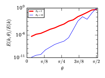
Figure 7: Plot of $E(k=20,\theta)/E(k=20)$ vs. $\theta$ for (a)${B_{0}}=2$ (thick line) and (b)${B_{0}}=10$ (thin line).

IV Energy flux and shell-to-shell energy transfers

In this section we will study energy transfers that provide insights into the two-dimensionalization process in MHD turbulence. To delve into the anisotropy of the flow and its causes, we investigate the energy flux and energy exchange between the perpendicular and parallel components of the velocity field. Earlier, energy transfers in the Fourier space have been studied in detail by various groups Dar et al. (2001); Verma (2004); Alexakis et al. (2005); Debliquy et al. (2005). Herein, we present an in-depth investigation of the energy transfers with comparatively stronger mean magnetic field amplitudes.

In hydrodynamics, for a basic triad of interacting wave-numbers $({\bf k},{\bf p},{\bf q})$ that satisfy ${\bf k}={\bf p}+{\bf q}$, the mode-to-mode energy transfer rate from the mode p to the mode k via mediation of the mode q is given by

$$S({\bf k}\mid{\bf p}\mid{\bf q})=\Im\{[{\bf k}\cdot{\bf\hat{u}({\bf q})}][{\bf\hat{u}}({\bf p})\cdot{\bf\hat{u}}^{*}({\bf k})]\},$$ (9)

where $\Im$ and $*$ denote respectively the imaginary part and complex conjugate of a complex number. To investigate the energy transfer rate from a set of wave numbers $\mathcal{D}_{p}$ to a set of wave numbers $\mathcal{D}_{k}$ we sum over all the possible triads ${\bf k}={\bf p}+{\bf q}$:

$$\mathcal{T}(\mathcal{D}_{k},\mathcal{D}_{p})=\sum_{{\bf k}\in\mathcal{D}_{k}}\sum_{{\bf p}\in\mathcal{D}_{p}}S({\bf k}\mid{\bf p}\mid{\bf q})=-\int{[\bf u_{k}(u\cdot\nabla)]u_{p}}dx^{3}$$ (10)

where $\bf u_{k}(x),u_{p}(x)$ express the velocity field filtered so that only the modes in $\mathcal{D}_{k},\mathcal{D}_{p}$ are kept respectably. The energy flux $\Pi(k_{0})$ then can be defined as the rate of energy transfer from the set $\mathcal{D}_{s}$ of modes inside a sphere of radius $k_{0}$ to modes outside the same sphere, i.e.,

$$\Pi(k_{0})=\sum_{k<k_{0}}\sum_{p\geq k_{0}}S({\bf k}\mid{\bf p}\mid{\bf q}).$$ (11)

Similarly we can define the shell-to-shell energy transfer rate $T_{n}^{m}=\mathcal{T}(\mathcal{D}_{n},\mathcal{D}_{m})$ as the energy transfer rate from the modes in a spherical shell $\mathcal{D}_{m}$ to the modes in the spherical shell $\mathcal{D}_{n}$.

MHD turbulence has six kinds of energy fluxes, namely the energy flux from inner u-sphere to outer u-sphere ($\Pi^{u<}_{u>}(k_{0})$), energy flux from inner u-sphere to outer b-sphere ($\Pi^{u<}_{b>}(k_{0})$), energy flux from inner b-sphere to outer b-sphere ($\Pi^{b<}_{b>}(k_{0})$), energy flux from inner b-sphere to outer u-sphere ($\Pi^{b<}_{u>}(k_{0})$), energy flux from inner u-sphere to inner b-sphere ($\Pi^{u<}_{b<}(k_{0})$), and energy flux from outer u-sphere to outer b-sphere ($\Pi^{u>}_{b>}(k_{0})$). These fluxes can be computed using the following formulae Verma (2004); Dar et al. (2001); Alexakis et al. (2005); Debliquy et al. (2005); Mininni et al. (2006):

$$\Pi^{u<}_{u>}(k_{0}) =\,\sum_{k<k_{0}}\sum_{p\leq k_{0}}\Im\{[{\bf k}\cdot{\bf\hat{u}({\bf q})}][{\bf\hat{u}}({\bf p})\cdot{\bf\hat{u}}^{*}({\bf k})]\}= +\int{\bf u}^{<}_{k}{\bf(u\cdot\nabla)}{\bf u}^{>}_{k}dx^{3},$$

$$\Pi^{u<}_{b>}(k_{0}) =-\sum_{k<k_{0}}\sum_{p\leq k_{0}}\Im\{[{\bf k}\cdot{\bf\hat{b}({\bf q})}][{\bf\hat{u}}({\bf p})\cdot{\bf\hat{b}}^{*}({\bf k})]\}= -\int{\bf u}^{<}_{k}{\bf(b\cdot\nabla)}{\bf b}^{>}_{k}dx^{3},$$

$$\Pi^{b<}_{u>}(k_{0}) =-\sum_{k<k_{0}}\sum_{p\leq k_{0}}\Im\{[{\bf k}\cdot{\bf\hat{b}({\bf q})}][{\bf\hat{b}}({\bf p})\cdot{\bf\hat{u}}^{*}({\bf k})]\}= -\int{\bf b}^{<}_{k}{\bf(b\cdot\nabla)}{\bf u}^{>}_{k}dx^{3},$$

$$\Pi^{b<}_{b>}(k_{0}) =\,\sum_{k<k_{0}}\sum_{p\leq k_{0}}\Im\{[{\bf k}\cdot{\bf\hat{u}({\bf q})}][{\bf\hat{b}}({\bf p})\cdot{\bf\hat{b}}^{*}({\bf k})]\}= +\int{\bf b}^{<}_{k}{\bf(u\cdot\nabla)}{\bf b}^{>}_{k}dx^{3}$$ (12)

where ${\bf u}^{<}_{k},{\bf b}^{<}_{k}$ express the velocity and magnetic fields where only the modes inside a sphere of radius $k$ are kept while ${\bf u}^{>}_{k},{\bf b}^{>}_{k}$ express the velocity and magnetic fields where only the modes outside the same sphere are kept. The total energy flux, which is the total energy transfer from the modes inside the sphere to the modes outside the sphere, is

$$\Pi(k_{0})=\Pi^{u<}_{u>}(k_{0})+\Pi^{u<}_{b>}(k_{0})+\Pi^{b<}_{u>}(k_{0})+\Pi^{b<}_{b>}(k_{0}).$$ (13)

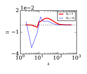
Figure 8: Plot of total energy flux $\Pi(k)$ vs. $k$.

In the present paper, we compute the energy fluxes for 19 concentric spheres with their centres at k = (0, 0, 0). The radii of the first three spheres are 2, 4, and 8, and those of the last two spheres are $512\times 2/3=170.5)$ and $r_{\mathrm{max}}=512\times 2/3=341$. Here the factor 2/3 is introduced due to dealiasing. The intermediate shells are based on the powerlaw expression

$$r_{i}=r_{3}\left[\frac{r_{\mathrm{max}}}{16.0}\right]^{\frac{i-3}{n-4}}.$$ (14)

where $r_{3}=8$ is radius of the third sphere, $r_{\mathrm{max}}$ is the radius of the last sphere, and $n=19$ is the total number of spheres. Hence, the radii of the spheres are 2.0, 4.0, 8.0, 9.8, 12.0, 14.8, 18.1, 22.2, 27.2, 33.4, 40.9, 50.2, 61.5, 75.4, 92.5, 113.4, 139.0, 170.5, and 341.0. In the inertial range we bin the radii of the shells logarithmically keeping in mind the powerlaw physics observed here. The inertial range however is too short since the forcing band is shifted to $k=[8,10]$.

For ${B_{0}}=2$ and 10, the total energy flux is shown in Fig. 8, while the individual fluxes (see Eq. (12)) are exhibited in Fig. 9. The plots are for a given snapshot during the evolved state. Due to aforementioned reason (lack of averaging) and relatively smaller resolution, we do not observe constant energy fluxes.

The most noticeable feature of the plots is the dominance of the inverse cascade of $\Pi^{u<}_{u>}(k_{0})$ for $k<k_{f}$ when ${B_{0}}=10$. This result is due to the quasi two-dimensionalization of the flow, and it is consistent with large kinetic energy at the large-scales near the equatorial region, discussed in the earlier section. The other energy fluxes are several orders of magnitudes smaller than the maximum value of $\Pi^{u<}_{u>}(k_{0})$.

In addition to the inverse cascade of kinetic energy, we observe that for $k>k_{f}$, all the energy fluxes are positive, which is consistent with the earlier results by Debliquy et al. Debliquy et al. (2005) for ${B_{0}}=0$. Interestingly, $\Pi^{b<}_{b>}<0$ for small wavenumbers ($k<k_{f}$) indicating inverse cascade of magnetic energy as well. It is important to note however that for $k>k_{f}$, $\Pi^{u<}_{u>}(k_{0})$ is the most dominant flux and it is positive. This is in contrast to the two-dimensional fluid turbulence in which the kinetic energy flux $\Pi^{u<}_{u>}\approx 0$ for $k>k_{f}$. The above feature is due to the forward energy transfer of $u_{\parallel}$.

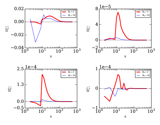
Figure 9: Plots of energy fluxes $\Pi^{u<}_{u>}$, $\Pi^{u<}_{b>}$, $\Pi^{b<}_{b>}$, and $\Pi^{b<}_{u>}$ vs. k.

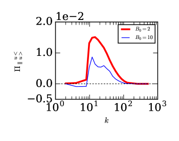
Figure 10: Plot of the energy flux ${\Pi_{\parallel}^{u}}$ of the parallel component of the velocity field, $u_{\parallel}$.

For anisotropic flows, Reddy et al. Reddy et al. (2014) showed how to compute energy fluxes for the parallel and perpendicular components of the velocity fields. They showed that these fluxes are

$$\Pi^{u}_{\parallel} = \sum_{k<k_{0}}\sum_{p>k_{0}}S_{\parallel}\left(\mathbf{k}\left|\mathbf{p}\right|\mathbf{q}\right)$$ (15)

$$\Pi^{u}_{\perp} = \sum_{k<k_{0}}\sum_{p>k_{0}}S_{\perp}\left(\mathbf{k}\left|\mathbf{p}\right|\mathbf{q}\right)$$ (16)

where

$$S^{u}_{\parallel}\left(\mathbf{{k}\left|{p}\right|{q}}\right) = \Im\left\{\left[\mathbf{k}\cdot\hat{\mathbf{u}}\left(\mathbf{q}\right)\right]\left[\hat{u}_{\parallel}^{\ast}\left(\mathbf{k}\right)\hat{u}_{\parallel}\left(\mathbf{p}\right)\right]\right\}$$ (17)

$$S^{u}_{\perp}\left(\mathbf{k}\left|\mathbf{p}\right|\mathbf{q}\right) = \Im\left\{\left[\mathbf{k}\cdot\hat{\mathbf{u}}\left(\mathbf{q}\right)\right]\left[\mathbf{\hat{u}_{\perp}^{\ast}\left({k}\right)\cdot\hat{u}_{\perp}\left({p}\right)}\right]\right\}$$ (18)

where $\Im$ and $*$ stand for the imaginary and complex conjugate of the arguments. Note that $\Pi^{u<}_{u>}=\Pi^{u}_{\parallel}+\Pi^{u}_{\perp}$. It is easy to derive the corresponding formulae for the magnetic energy by replacing $\hat{u}_{\parallel}$ and $\mathbf{\hat{u}_{\perp}}$ in Eqs. (17, 18) by $\hat{b}_{\parallel}$ and $\mathbf{\hat{b}_{\perp}}$ respectively. In this paper, we report the above fluxes only for the velocity field since the magnetic energy is much smaller than the kinetic energy. In Fig. 10 we plot $\Pi^{u}_{\parallel}$ that exhibits a forward energy cascade of $u_{\parallel}$ at large wavenumbers. The energy flux of the perpendicular component, $\Pi^{u}_{\perp}$ (not shown here), exhibits inverse cascade. The above observation is very similar to the quasi two-dimensional behaviour reported for quasi-static MHD turbulence by Reddy et al. Reddy et al. (2014) and Favier et al. Favier et al. (2010)— $\mathbf{\hat{u}_{\perp}}$ exhibiting an inverse cascade at low wavenumbers, while $u_{\parallel}$ a forward cascade at large wavenumbers. We further note that kinetic helicity $H=\langle\bf u\cdot\nabla\times u\rangle$ in this quasi two-dimensional is a result of the correlation of the vertical velocity and the two dimensional vorticity $w_{z}=\partial_{x}u_{y}-\partial_{y}u_{x}$ thus the forward cascade of helicity is controlled by the forward cascade of the energy of the vertical component. The forward cascade of Helicity has been shown recently to alter the exponent of the energy spectrum Sujovolsky and Mininni (2016).

However $E^{\perp}_{u}$ and $E^{\parallel}_{u}$ are not independently conserved quantities. $E^{\perp}_{u}$ energy can be transferred to $E^{\parallel}_{u}$ and vice versa via pressure. This transfer can be quantified by

$$\mathcal{P}_{\parallel}({\bf k})=\Im\left\{[k_{\parallel}\hat{u}_{\parallel}({\bf k})]P({\bf k})\right\}$$ (19)

as shown in Reddy et al. (2014). A sum of the above over a wavenumber shell yields energy transfer from ${\bf u}_{\perp}$ to $u_{\parallel}$ for that shell. The above energy transfer, plotted in Fig. 11, reveals that this energy transfer is relatively weak for ${B_{0}=10}$. This feature may be due to relatively weak pressure and velocity fields. The energy transfer from ${\bf u}_{\perp}$ to $u_{\parallel}$ enhances $E^{\parallel}_{u}$, which is advected to larger wavenumbers. Such features have been observed for quasi-static MHD Reddy et al. (2014). The energy of the perpendicular component ($E^{\perp}_{u}$) however grows in the large scales in the presence of an inverse cascade. This is not very significant for $B_{0}=2$ that has no inverse cascade, but it is dominant for $B_{0}=10$. Thus, $E^{\parallel}_{u}\sim E^{\perp}_{u}$ for $B_{0}=2$, but $E^{\parallel}_{u}\ll E^{\perp}_{u}$ for $B_{0}=10$ (see Table I). As describe above and exhibited in Fig. 10, $u_{\parallel}$ cascades forward to larger wavenumbers, which is the cause for the $A_{u}(k)=E_{u}^{\perp}(k)/(2E_{u}^{\parallel}(k))<1$ for large $k$. We also observe that the energy transfers for the magnetic field may be coupled to the above transfers of the kinetic energy; this aspect needs to be investigated in detail.

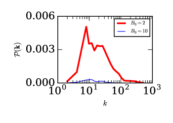
Figure 11: Plot of $\mathcal{P}_{\parallel}({\bf k})$, the energy transfer rate from $u_{\perp}$ to $u_{\parallel}$ via pressure.

Figure 12: Shell-to-shell energy transfers (a) $U2U$, (b) $B2B$, and (c) $U2B$ for ${B_{0}=2}$(left column) and ${B_{0}=10}$(right column). Here $m$ is the giver shell, and $n$ is the receiver shell.

The energy flux describes the net energy emanating from a sphere. More details on energy transfer is revealed by the shell-to-shell energy transfer rates. For fluid turbulence, we have shell-to-shell transfers for the velocity field. However, for MHD turbulence we have velocity-to-velocity ($U2U$), magnetic-to-magnetic ($B2B$), and kinetic-to-magnetic ($U2B$) shell-to-shell energy transfers Dar et al. (2001); Alexakis et al. (2005); Debliquy et al. (2005); Teaca et al. (2009). The energy transfer from wavenumber shell $m$ of field $X$ to wavenumber shell $n$ of field $Y$ is defined as ($X,Y$ are either velocity or magnetic field):

$$\mathcal{T}^{u,u}_{n,m} = \sum_{k\in\mathcal{D}_{n}}\sum_{p\in\mathcal{D}_{m}}\Im\{[{\bf k}\cdot{\bf\hat{u}({\bf q})}][{\bf\hat{u}}({\bf p})\cdot{\bf\hat{u}}^{*}({\bf k})]\}=-\int{[\bf u_{k}(u\cdot\nabla)]u_{p}}dx^{3}$$ (20)

$$\mathcal{T}^{b,b}_{n,m} = \sum_{k\in\mathcal{D}_{n}}\sum_{p\in\mathcal{D}_{m}}\Im\{[{\bf k}\cdot{\bf\hat{u}({\bf q})}][{\bf\hat{b}}({\bf p})\cdot{\bf\hat{b}}^{*}({\bf k})]\}=-\int{[\bf b_{k}(u\cdot\nabla)]b_{p}}dx^{3}$$ (21)

$$\mathcal{T}^{b,u}_{n,m} = -\sum_{k\in\mathcal{D}_{n}}\sum_{p\in\mathcal{D}_{m}}\Im\{[{\bf k}\cdot{\bf\hat{u}({\bf q})}][{\bf\hat{u}}({\bf p})\cdot{\bf\hat{b}}^{*}({\bf k})]\}=+\int{[\bf b_{k}(b\cdot\nabla)]u_{p}}dx^{3}$$ (22)

For the shell-to-shell energy transfers we divide the wavenumber space into 19 concentric shells with their centres at k = (0, 0, 0). The inner and outer radii of the $n$th shell are $k_{n-1}$ and $k_{n}$ respectively, where $k_{n}=0$, 2.0, 4.0, 8.0, 9.8, 12.0, 14.8, 18.1, 22.2, 27.2, 33.4, 40.9, 50.2, 61.5, 75.4, 92.5, 113.4, 139.0, 170.5, and 341.0. The aforementioned radii are chosen using the same algorithm as those used for the computing the radii of the spheres for the flux computations. In Fig. 12, we present the shell-to-shell energy transfer rates, $T^{uu}_{nm}$, $T^{bb}_{nm}$, and $T^{bu}_{nm}$ for $B_{0}=2$ (left column) and $B_{0}=10$ ( right column).

The $U2U$ and $B2B$ transfers for ${B_{0}}=2$, exhibited in Fig. 12(a) is similar to those reported by Alexakis et al. Alexakis et al. (2005), Debliquy et al. Debliquy et al. (2005), and  Carati et al. Carati et al. (2006) for ${B_{0}}=0$ forward and local $U2U$ and $B2B$ transfers, that is, the most energy transfers are from shell $m-1$ to shell $m$. The $U2B$ transfer is from shell $m$ of the velocity field to shell $m$ of the magnetic field, which is because the velocity field dominates the magnetic field Debliquy et al. (2005); this feature is exactly opposite to that for ${B_{0}}=0$ Alexakis et al. (2005); Debliquy et al. (2005); Carati et al. (2006) because $E_{b}>E_{u}$ for the ${B_{0}}=0$ case.

For ${B_{0}=10}$ (see Fig. 12), $U2U$is the most dominant transfer, and the $U2U$ and $B2B$ shell-to-shell transfer exhibits inverse energy transfers for the 3rd and 4th shell ($k<k_{f}$), i.e., from the 4th shell to the 3rd shell. This result is consistent with the inverse cascades of kinetic and magnetic energies for $k<k_{f}$ (see Fig. 9). The $U2B$ transfers are nonzero only for $k<k_{f}$.

V Summary and Discussion

In this paper we analyzed the anisotropy induced by a constant magnetic field in MHD turbulence. Here we provide semiquantitative picture of the above phenomena. Shear Alfvén modes are linear excitations of MHD flows, and they are governed by equations:

$$\frac{d\hat{\bf u}({\bf k})}{dt}=i({\bf B_{0}\cdot k})\hat{\bf b}({\bf k});~{}~{}~{}\frac{d\hat{\bf b}({\bf k})}{dt}=i({\bf B_{0}\cdot k})\hat{\bf u}({\bf k})$$ (23)

The above equations have valid wave solutions when ${\bf B_{0}\cdot k}\neq 0$, that is, for wave vectors off from the plane perpendicular to the mean magnetic field. For such modes, in Eq. (4,5), $({\bf B}_{0}\cdot{\bf k}){\bf u(k)}$ and $({\bf B}_{0}\cdot{\bf k}){\bf b(k)}$ dominates the nonlinear term. Earlier, Galtier et al. Galtier et al. (2000) had analysed the weak turbulence limit of MHD turbulence for large ${B_{0}}$ and showed that $E(k_{\perp})\sim k_{\perp}^{-2}$.

For the Fourier modes with $k_{\parallel}=0$, the linear terms dropout of Eqs. (4,5) and the nonlinear terms dominate the flow with dynamics. In addition, for large $B_{0}$, $b^{2}\ll u^{2}$ (see Table I). Since $k_{\parallel}=0$ for such modes, the modes have interactions similar to two-dimensional hydrodynamic turbulence. These interactions lead to two-dimensionalization of the flow. The reason for $b^{2}\ll u^{2}$ is unclear at present, but it may be due to the absence of share Alfvén waves for modes with $k_{\parallel}=0$. To sum up, for the Fourier modes with $k_{\parallel}\neq 0$, we obtain Alfvénic fluctuations, which are described by Eqs. (23) in the linear limit. However, for large $B_{0}$, the fluctuations corresponding to these modes are weak compared to the vortical structures. Thus the flow is dominated by the $k_{\parallel}=0$ modes. These arguments provide qualitative picture for the emergence of quasi two-dimensional vortices in MHD turbulence with strong $B_{0}$. The above behaviour has strong similarities with the vortical structures observed in rotating and quasi-static MHD turbulence Reddy and Verma (2014).

The dominance of these modes leads then to an anisotropic distribution of the velocity components with the perpendicular components dominating in the large scales due to the inverse cascade of $E_{\perp}$ while the parallel components dominate in the small scales due to the forward cascade of $E_{\parallel}$. This leads to the formation of the observed vortical structures.

In summary, we show how strong mean magnetic field makes the MHD turbulence quasi two-dimensional. This conclusion is borne out in the global-energy anisotropy parameter, ring spectrum, energy flux, and shell-to-shell energy transfers. The flow has strong similarities with those observed in rotating and quasi-static MHD turbulence. Detailed dynamical connections between these flows need to be explored in a future work.

VI Acknowledgments

We thank Sandeep Reddy, Abhishek Kumar, Biplab Dutta and Rohit Kumar for valuable discussions. Our numerical simulations were performed at HPC2013 and Chaos clusters of IIT Kanpur. This work was supported by the research grants 4904-A from Indo-French Centre for the Promotion of Advanced Research (IFCPAR/CEFIPRA), SERB/F/3279/2013-14 from the Science and Engineering Research Board, India, and Project A9 via SFB-TR24 from DFG Germany.

References

- Alexakis (2013) A. Alexakis, Phys. Rev. Lett. 110, 084502 (2013).
- Iroshnikov (1963) P. S. Iroshnikov, Soviet Astronomy 40, 742 (1963).
- Kraichnan (1965) R. H. Kraichnan, Physics of Fluids 8, 1385 (1965).
- Shebalin et al. (1983) J. V. Shebalin, W. H. Matthaeus, and D. Montgomery, J. Plasma Physics 29, 525 (1983).
- Zank and Matthaeus (1993) G. P. Zank and W. Matthaeus, Physics of Fluids A: Fluid Dynamics (1989-1993) 5, 257 (1993).
- Oughton et al. (1994) S. Oughton, E. R. Priest, and W. H. Matthaeus, Journal of Fluid Mechanics 280, 95 (1994).
- Verma (1999) M. K. Verma, Phys. Plasmas 6, 1455 (1999).
- Verma (2004) M. K. Verma, Physics reports 401, 229 (2004).
- Verma (2001) M. Verma, Phys. Rev. E 64, 26305 (2001).
- Goldreich and Sridhar (1995) P. Goldreich and S. Sridhar, The Astrophysical Journal 438, 763 (1995).
- Boldyrev (2006) S. Boldyrev, Phys. Rev. Lett. 96, 115002 (2006).
- Boldyrev and Perez (2009) S. Boldyrev and J. C. Perez, Physical Review Letters 103, 225001 (2009).
- Perez et al. (2012) J. C. Perez, J. Mason, S. Boldyrev, and F. Cattaneo, Phys. Rev. X 2, 041005 (2012).
- Perez et al. (2014) J. C. Perez, J. Mason, S. Boldyrev, and F. Cattaneo, Astrophys. J. Lett. 793, L13 (2014).
- Beresnyak and A. (2009) A. Beresnyak and L. A., Astrophys. J 702, 1190 (2009).
- Beresnyak (2011) A. Beresnyak, Physical Review Letters 106, 075001 (2011).
- Beresnyak (2014) A. Beresnyak, Astrophys. J. Lett. 784, L20 (2014).
- Galtier et al. (2000) S. Galtier, S. V. Nazarenko, A. C. Newell, and A. Pouquet, J. of Plasma Physics 63, 447 (2000).
- Alexakis (2011) A. Alexakis, Phys. Rev. E 84, 056330 (2011).
- Reddy and Verma (2014) K. S. Reddy and M. K. Verma, Physics of Fluids 26, 025109 (2014).
- Reddy et al. (2014) K. S. Reddy, R. Kumar, and M. K. Verma, Physics of Plasmas 21, 102310 (2014).
- Gallet and Doering (2015) B. Gallet and C. R. Doering, Journal of Fluid Mechanics 773, 154 (2015).
- Alexakis et al. (2007) A. Alexakis, B. Bigot, H. Politano, and S. Galtier, Phys. Rev. E 76, 056313 (2007).
- Teaca et al. (2009) B. Teaca, M. K. Verma, B. Knaepen, and D. Carati, Phys. Rev. E 79, 046312 (2009).
- Roberts (1967) P. H. Roberts, An Introduction to Magnetohydrodynamics (New York: Elsevier, 1967).
- Mininni et al. (2011) P. D. Mininni, D. Rosenberg, R. Reddy, and A. Pouquet, Parallel Computing 37, 316 (2011).
- Verma et al. (2013) M. K. Verma, A. Chatterjee, K. S. Reddy, R. K. Yadav, S. Paul, M. Chandra, and R. Samtaney, Pramana 81, 617 (2013).
- Favier et al. (2010) B. Favier, F. S. Godeferd, C. Cambon, and A. Delache, Physics of Fluids 22, 075104 (2010).
- TenBarge et al. (2012) J. M. TenBarge, J. J. Podesta, K. G. Klein, and G. G. Howes, The Astrophysical Journal 753, 107 (2012).
- Alexandrova et al. (2008) O. Alexandrova, V. Carbone, P. Veltri, and L. Sorriso-Valvo, The Astrophysical Journal 674, 1153 (2008).
- Dar et al. (2001) G. Dar, M. K. Verma, and V. Eswaran, Physica D: Nonlinear Phenomena 157, 207 (2001).
- Alexakis et al. (2005) A. Alexakis, P. D. Mininni, and A. Pouquet, Phys. Rev. E 72, 046301 (2005).
- Debliquy et al. (2005) O. Debliquy, M. K. Verma, and D. Carati, Physics of Plasmas 12, 042309 (2005).
- Mininni et al. (2006) P. D. Mininni, A. G. Pouquet, and D. C. Montgomery, Phys. Rev. Lett. 97, 244503 (2006).
- Sujovolsky and Mininni (2016) N. E. Sujovolsky and P. D. Mininni, ArXiv e-prints (2016), eprint 1606.04026.
- Carati et al. (2006) D. Carati, O. Debliquy, B. Knaepen, B. Teaca, and M. K. Verma, Journal of Turbulence 7, N51 (2006).