Masses and decay constants of the $D_{s0}^{*}(2317)$ and $D_{s1}(2460)$ from $N_{f}=2$ lattice QCD close to the physical point

Abstract

We perform a high statistics study of the $J^{P}=0^{+}$ and $1^{+}$ charmed-strange mesons, $D_{s0}^{*}(2317)$ and $D_{s1}(2460)$, respectively. The effects of the nearby $DK$ and $D^{*}K$ thresholds are taken into account by employing the corresponding four quark operators. Six ensembles with $N_{f}=2$ non-perturbatively ${\cal O}(a)$ improved clover Wilson sea quarks at $a=0.07$ fm are employed, covering different spatial volumes and pion masses: linear lattice extents $L/a=24,32,40,64$, equivalent to 1.7 fm to 4.5 fm, are realised for $m_{\pi}=290$ MeV and $L/a=48,64$ or 3.4 fm and 4.5 fm for an almost physical pion mass of $150$ MeV. Through a phase shift analysis and the effective range approximation we determine the scattering lengths, couplings to the thresholds and the infinite volume masses. Differences relative to the experimental values are observed for these masses, however, this is likely to be due to discretisation effects as spin-averaged quantities and splittings are reasonably compatible with experiment. We also compute the weak decay constants of the scalar and axialvector and find $f_{V}^{0^{+}}=114(2)(0)(+5)(10)$ MeV and $f_{A}^{1^{+}}=194(3)(4)(+5)(10)$ MeV, where the errors are due to statistics, renormalisation, finite volume and lattice spacing effects.

I Introduction

In 2003 the BABAR Collaboration announced the observation of a meson state in the inclusive $D_{s}^{+}\pi^{0}$ invariant mass distribution Aubert et al. (2003), compatible with a $J^{P}=0^{+}$ assignment, the $D_{s0}^{*}(2317)$. This discovery was confirmed soon after by the CLEO and Belle Collaborations Besson et al. (2004); Krokovny et al. (2003). The newfound state was the natural candidate to fill in the charm-strange $0^{+}$ $P$-wave level predicted by quark models. However, while quark models Godfrey and Isgur (1985); Godfrey and Kokoski (1991) and a number of early lattice calculations Lewis and Woloshyn (2000); Hein et al. (2000); Bali (2003); Dougall et al. (2003) based on quark-antiquark interpolators predicted the $0^{+}$ state to be a broad resonance above the nearby $DK$ threshold, the experiments observed a narrow state of mass $2317$ MeV, $40$ MeV below threshold. The detection of another narrow state just below the $D^{*}K$ threshold, the $D_{s1}(2460)$ Besson et al. (2003); Mikami et al. (2004); Aubert et al. (2004) with $J^{P}=1^{+}$, presented a similar puzzle.

The strange-charm meson sector can be interpreted within heavy quark effective theory Isgur and Wise (1991); Nowak et al. (1993); Bardeen and Hill (1994); Neubert (1994); Ebert et al. (1995); Bardeen et al. (2003) (HQET). At leading order in the inverse of the heavy quark mass, the states are arranged in degenerate doublets corresponding to the strange quark quantum numbers: $j^{P}=\frac{1}{2}^{-}$ for angular momentum $l=0$ and $j^{P}=\frac{1}{2}^{+}$ and $\frac{3}{2}^{+}$ for $l=1$ and so on. Interactions beyond leading order, including with the heavy (charm) quark spin, lift the degeneracies and cause mixing between $j^{P}=\frac{1}{2}^{+}$ and $\frac{3}{2}^{+}$ states. The relevant quantum numbers are then the total quark and antiquark spin, i.e. $J^{P}=0^{-}$, $1^{-}$, for the $l=0$ doublet and $0^{+}$, $1^{+}$ and $1^{+}$, $2^{+}$ for $l=1$. The doublets can be (loosely) identified with the observed $\left(D_{s},D_{s}^{*}\right)$, $\left(D_{s0}^{*}(2317),D_{s1}\left(2460\right)\right)$ and $\left(D_{s1}\left(2536\right),D_{s2}^{*}(2573)\right)$ mesons, respectively. Nevertheless, the surprisingly low masses of the $D_{s0}^{*}(2317)$ and $D_{s1}\left(2460\right)$ mesons have led to a number of more exotic interpretations, for example, as tetraquarks Barnes et al. (2003); Terasaki (2003); Chen and Li (2004), molecules Cheng and Hou (2003); Browder et al. (2004) or conventional charm-strange mesons with coupled channel effects van Beveren and Rupp (2003). A recent comprehensive review of the experimental status and theoretical understanding of these states can be found in Ref. Chen et al. (2017).

Subsequent lattice studies Mohler and Woloshyn (2011); Namekawa et al. (2011); Moir et al. (2013), utilising quark-antiquark interpolators and, most recently, including chiral and continuum extrapolations Cichy et al. (2016) also overestimate the mass of the $D_{s0}^{*}(2317)$. A similarly conventional analysis by some of us found consistency with the $0^{+}$ and $1^{+}$ $D_{s}$ experimental masses in Ref. Perez-Rubio et al. (2015), however, there were a number of systematic uncertainties that could not be quantified. The possible influence of the nearby threshold needs to be taken into account by incorporating four-quark $DK$ interpolators and performing a finite volume analysis utilising Lüscher’s formalism Lüscher (1991) for the unequal mass case Davoudi and Savage (2011); Fu (2012); Leskovec and Prelovsek (2012). The first work in this direction was performed by Liu and collaborators who computed the scattering lengths for the $D\overline{K}$ system for which there are no computationally challenging disconnected diagrams Liu et al. (2013). Predictions were made for the $DK$ channel via SU(3) flavour symmetry. Following this, Mohler et al. Mohler et al. (2013) and Lang et al. Lang et al. (2014) studied the $D_{s0}^{*}(2317)$ and $D_{s1}(2460)$ mesons directly, including coupling with the threshold, and found their masses to be compatible with experiment for an ensemble with $m_{\pi}=156$ MeV, at a fairly coarse lattice spacing of $a=0.09$ fm and a small spatial lattice extent of $L=2.9$ fm ($Lm_{\pi}=2.29$). The effective range approximation was assumed in order to extract infinite volume results. Notably, the masses of these states were found to be overestimated if the $DK$ interpolators were omitted.

Clearly, a number of improvements can be made on this pioneering study working, for example, at a finer lattice spacing and exploring the dependence on the spatial volume. The former is important since discretisation effects can be substantial for observables involving charm quarks while the latter is needed as contributions which are exponentially suppressed in $Lm_{\pi}$ (that are ignored in the Lüscher formalism) may not be small for $Lm_{\pi}=2.29$. Furthermore, the range of validity of the effective range approximation needs to be tested.

In this work we present a high statistics analysis at $a=0.07$ fm for two pion masses, $m_{\pi}=290$ and 150 MeV, utilising multiple spatial volumes, with $L$ in the range of $1.7$ to 4.5 fm realising values for $Lm_{\pi}$ between $2.7$ to $6.7$. Near to physical pion masses are required as the $0^{+}$ and $1^{+}$ charm-strange states are sensitive to the position of the threshold and one needs to reproduce the physical case. By employing $N_{f}=2$ dynamical fermions, effects arising from strange sea quarks are omitted with the expectation that the valence strange quark provides the dominant contribution. Furthermore, we treat the $D_{s0}^{*}(2317)$ and $D_{s1}(2460)$ as stable and ignore their (strong) decays to $D_{s}\pi$ and $D_{s}^{*}\pi$ and $D_{s}\pi\pi$, respectively. This is reasonable, given that the first two decays are isospin-violating (and in our simulation isospin is exact) and the third has a very small width. Effects of the higher lying $D_{s}\eta$ and $D^{*}_{s}\eta$ thresholds are also neglected.

Table 1: Details of the ensembles used for this analysis. $Lm_{\pi}$ is computed using the infinite volume pion mass determined in Ref. Bali et al. (2015).

$\kappa_{l}$	$a$ [fm]	$V$	$am_{\pi}$	$m_{\pi}$ [MeV]	$Lm_{\pi}$	$m_{K}$ [MeV]	$m_{D}$ [MeV]	$m_{D^{*}}$ [MeV]	$N_{\rm conf}$
0.13632	0.071	$24^{3}\times 48$	0.1112(9)	306.9(2.5)	2.67	$540(2)$	$1907(3)$	$2038(5)$	$2222$
	0.071	$32^{3}\times 64$	0.10675(52)	294.6(1.4)	3.42	$528(1)$	$1902(3)$	$2030(5)$	$1453$
	0.071	$40^{3}\times 64$	0.10465(38)	288.8(1.1)	4.19	$527(1)$	$1901(2)$	$2030(4)$	$2000$
	0.071	$64^{3}\times 64$	0.10487(24)	289.5(0.7)	6.70	$526(1)$	$1898(1)$	$2030(2)$	$1463$
0.13640	0.071	$48^{3}\times 64$	0.05786(55)	159.7(1.5)	2.78	$500(1)$	$1880(2)$	$2007(3)$	$2501$
	0.071	$64^{3}\times 64$	0.05425(49)	149.7(1.4)	3.49	$497(1)$	$1877(1)$	$1996(3)$	$1591$

So far, most lattice studies have focused on computing the particle masses and the couplings of the states to the two meson channels. In this work, we also determine the weak decay constants, i.e. the overlap of the (local) weak current operator with the physical state, for $J^{P}=0^{+}$ and the lower $1^{+}$ meson. The decay constants have not yet been directly determined in experiment, however, some information can be extracted from non-leptonic $B$ decays to $D^{(*)}D_{sJ}^{(*)}$. Within the factorisation approximation, invoking the heavy quark limit Beneke et al. (2000); Luo and Rosner (2001), ratios of the corresponding branching fractions give $f_{D_{s0}^{*}(2317)}\sim f_{Ds}/3$, while for the axialvector channel $f_{D_{s1}(2460)}\sim 2f_{D^{*}_{s}}/3$, see, for example, the analyses of Refs. Datta and O’Donnell (2003); Hwang and Kim (2005); Cheng and Chua (2006). These results, however, are at odds with heavy quark symmetry studies which find $f_{D_{s1}(2460)}\sim f_{D_{s0}^{*}(2317)}$ Colangelo et al. (1999); Le Yaouanc et al. (2001); Colangelo and De Fazio (2002). The decay constants have also been computed, for example, within quark models Le Yaouanc et al. (2001); Cheng et al. (2004); Hsieh et al. (2004); Verma (2012); Segovia et al. (2012) and QCD sum rules Colangelo et al. (2005); Wang (2015) with results covering a wide range, $f_{D_{s0}^{*}(2317)}=70-440$ MeV and $f_{D_{s1}(2460)}=117-410$ MeV.

The paper is organised as follows. Details of the lattice set-up are given in Section II. The construction of the quark line diagrams required for extracting the energy levels and matrix elements for the states of interest are discussed in Section III. The procedure for extracting the phase shifts, the couplings to the two meson channels and the masses from the finite volume levels is well established and we only provide a brief overview of the theoretical background in Section IV. We extract the infinite volume information employing two methods: Lüscher’s formalism Lüscher (1991); Davoudi and Savage (2011); Fu (2012); Leskovec and Prelovsek (2012) as well as the chiral unitary approach Oller and Oset (1997); Oller et al. (1998), which also allows us to determine the so-called potential of the scattering particles. Our results on the phase shifts, scattering lengths, potentials, spectrum and decay constants are presented in Section V, before we conclude in Section VI.

II Lattice set-up

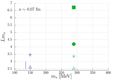
Figure 1: Overview of the ensembles employed in our analysis in terms of the pion mass and the spatial extent $L$ (in units of $m_{\pi}$). The vertical line indicates the physical pion mass.

In order to study the volume dependence of the lowest lying energy levels, various spatial volumes are realised at two pion masses, $m_{\pi}\sim 290$ MeV with $L/a=24,32,40,64$ and $m_{\pi}\sim 150$ MeV with $L/a=48,64$, where $L$ denotes the linear extent. The ensembles were generated by the RQCD and QCDSF collaborations and are composed of $N_{f}=2$ non-perturbatively improved clover fermions at a single lattice spacing $a=0.071$ fm Bali et al. (2015) (determined via the Sommer scale $r_{0}$ Sommer (1994)). Details of the ensembles are given in Table 1 and Fig. 1. The strange and charm quarks are partially quenched in our analysis and their masses are fixed by reproducing (to within 1$\%$) the combination $\sqrt{2m_{K}^{2}-m_{\pi}^{2}}=685.8$ MeV employing the electrically neutral, isospin-averaged estimates from the FLAG review Aoki et al. (2017) (see the discussion below) and the experimental value of the spin-averaged $1S$ charmonium mass, $m_{1S}=3068.5$ MeV, respectively. When computing the latter we omit disconnected quark line diagrams and mixing with other flavour singlets. The effect of this omission is likely to be only a few MeV in the $1S$ charmonium mass (see, for example, the studies in Refs. Levkova and DeTar (2011); Bali et al. (2011)) and does not lead to a significant uncertainty in our results for the $D_{s}$ spectrum.

As mentioned previously, reproducing the physical $DK$ and $D^{*}K$ thresholds is important for studying the $0^{+}$ and $1^{+}$ states, respectively. In order to compare our lattice values for these thresholds and other levels with experiment, however, corrections are required as we are working in the isospin limit and electromagnetic effects are absent. We choose to adjust the experimental results rather than correcting the lattice values. For the kaon we take the FLAG review Aoki et al. (2017) value of $m_{K}^{\rm QCD}=494.2(3)$ MeV for the physical mass in QCD. For the $D^{(*)}$ mesons we define the electrically neutral isospin symmetric mass as,

$$m^{\rm QCD}_{D^{(*)}}=\frac{1}{2}\left(m_{D^{(*)0}}+m_{D^{(*)\pm}}-\delta m_{D^{(*)}}^{\rm QED}\right).$$ (1)

The electromagnetic mass contributions, $\delta m_{D}^{\rm QED}=2.3(2)$ MeV and $\delta m_{D^{*}}^{\rm QED}=0.8(2)$ MeV were estimated in Ref. Goity and Jayalath (2007) in the heavy quark limit including $1/m_{Q}$ terms. To be conservative we double the size of these QED errors. Combining these values with the experimental masses gives $m^{\rm QCD}_{D}=1866.1(2)$ MeV and $m^{\rm QCD}_{D^{*}}=2008.2(2)$ MeV. For the $D_{s}^{(*)}$ mesons the electromagnetic mass contribution is assumed to be of the same size as for the $D$ mesons with,

$$m^{\rm QCD}_{D_{s}^{(*)}}=m_{D_{s}^{(*)}}-\delta m_{D^{(*)}}^{\rm QED},$$ (2)

giving $m_{D_{s}}^{\rm QCD}=1966.0(4)$ MeV and $m_{D_{s}}^{\rm QCD}=2111.3(6)$ MeV. No estimates have been made of $\delta m^{\rm QED}$ for the positive parity charm-strange mesons and in this case we add an additional error of 2 MeV to the experimental masses to indicate the likely size of this uncertainty. So, for example, we quote for the $0^{+}$ mass, $m_{0^{+}}=2317.7(0.6)(2.0)$ MeV, where the first error is experimental, while for the splitting with the threshold we give $m_{K}+m_{D}-m_{0^{+}}=42.6(0.7)(2.0)$ MeV, with the first error due to the QCD estimate of $m_{K}+m_{D}$. Turning to the lattice data in Table 1 for the $m_{\pi}=150$ MeV, $L=64a$ ensemble, the kaon mass is compatible with the FLAG estimate, while the $D$ ($D^{*}$) meson mass is slightly above (below) the QCD value. This leads to the $DK$ and $D^{*}K$ thresholds being missed by only $+14$ and $-9$ MeV, respectively.

Leading order discretisation effects are of $\mathcal{O}(a^{2})$ and, as the charm quark mass in lattice units is not small ($am_{c}\sim 0.5$), lattice spacing effects can be significant. Fine structure splittings are expected to be particularly sensitive to such effects as they are dominated by momentum scales close to $m_{c}$ for heavy-light systems. This is illustrated by our results for the $D$ and $D_{s}$ $1S$ hyperfine splittings, $m_{D^{*}}-m_{D}=119(3)$ MeV and $m_{D_{s}^{*}}-m_{D_{s}}=118(1)$ MeV, from the largest $m_{\pi}=150$ MeV ensemble, which are approximately 23 MeV and 27 MeV below the corrected experimental values, respectively. In contrast, spin-averaged splittings which have typical energy scales that are much smaller than the inverse lattice spacing (of the order of $\overline{\Lambda}\sim 0.5$ GeV for heavy-light systems which is much less than $a^{-1}=2.76$ GeV), are less affected as will be demonstrated in Section V.

We perform a high statistics study utilising 1450 to 2200 configurations for each ensemble, see Table 1. Careful consideration of auto-correlations is required and these were taken into account by binning over measurements (one per configuration) to a level consistent with at least four times the integrated auto-correlation time.

Finite volume effects on hadron masses and decay constants fall off exponentially with $Lm_{\pi}$ and empirically $Lm_{\pi}>4$ has been found to be sufficient for such effects to be suppressed in most observables. In Lüscher’s formalism smaller volumes are beneficial for obtaining infinite volume information, however, the exponentially suppressed finite volume terms are neglected and $Lm_{\pi}$ cannot be too small. This will be discussed in Section V; for our ensembles $Lm_{\pi}$ ranges from 2.67 to 6.71.

III Correlator matrix

Two distinct sectors corresponding to $J^{P}=0^{+}$ and $1^{+}$ are considered in this work. In the first case, the lowest energy level is expected to coincide with the bound state $D_{s0}^{*}(2317)$, followed by a $DK$ scattering state somewhat above. Analogously, in the second case we expect to find the $D_{s1}(2460)$, followed by a $D^{*}K$ scattering state as well as the $D_{s1}(2536)$.

In order to extract these levels a variational analysis is performed Michael (1985); Lüscher and Wolff (1990). Choosing a set of quark-antiquark and two meson interpolators $O_{i}$ which have an overlap $Z_{kj}=\braket{k}{O_{j}^{\dagger}}{0}$ with the physical states of interest, $\ket{k}$, a correlator matrix is constructed,

$$C_{ij}\left(t\right)=\braket{0}{O_{i}\left(t\right)O_{j}^{\dagger}}{0}=\sum_{k}Z_{ik}^{\dagger}Z_{kj}e^{-E_{k}t}.$$ (3)

Note that the interpolators are projected onto zero momentum. By solving the generalised eigenvalue equation

$$C\left(t\right)v^{\left(k\right)}(t,t_{0})=\lambda^{\left(k\right)}\left(t,t_{0}\right)C\left(t_{0}\right)v^{\left(k\right)}(t,t_{0})$$ (4)

for eigenvalues $\lambda^{\left(k\right)}(t,t_{0})$ and eigenvectors $v^{\left(k\right)}(t,t_{0})$ for $t>t_{0}$, $t_{0}$ being a reference time, the energy levels are obtained from the exponential decay of the eigenvalues

$$\lambda^{\left(k\right)}\left(t,t_{0}\right)=e^{-E_{k}\left(t-t_{0}\right)}\left(1+\mathcal{O}\left(e^{-\Delta E_{k}t}\right)\right),$$ (5)

where $\Delta E_{k}$ is the difference between $E_{k}$ and the first energy level outside of the rank of the basis considered for $t<2t_{0}$ and $t-t_{0}$ constant Blossier et al. (2009). Clearly, the basis of operators must be large enough in order to resolve the number of levels of interest, and in general, due to the contamination from higher states one needs a basis of at least $n+1$ operators in order to reliably extract $n$ states.

The choice of operators is also important, especially for the charm-strange systems of interest here where the lowest two energy levels are very close to each other (in particular for the larger spatial volumes): a basis of operators with poor overlap with the physical states will not separate the energy levels within the finite (Euclidean) time extent of the lattice. This is precisely the problem when forming a basis of only $\bar{q}q$ interpolators, which leads to the overestimation of the mass of both the lowest $0^{+}$ and $1^{+}$ $D_{s}$ states as illustrated in Refs. Mohler et al. (2013); Lang et al. (2014) and demonstrated again in Section V.1.

Table 2: Interpolators used in the analysis.

$J^{P}$	Two-quark operators
$0^{+}$	$O_{D_{s}}=\overline{s}\mathbb{1}c,\quad O_{D^{\prime}_{s}}=\overline{s}\gamma_{t}c$
$1^{+}$	$O_{D_{s}}=\overline{s}\gamma_{i}\gamma_{5}c,\quad O_{D^{\prime}_{s}}=\overline{s}\gamma_{t}\gamma_{i}\gamma_{5}c$
$J^{P}$	Four-quark operators
$0^{+}$	$O_{DK}=\left(\overline{u}\gamma_{5}c\right)\left(\overline{s}\gamma_{5}u\right)+\left(\overline{d}\gamma_{5}c\right)\left(\overline{s}\gamma_{5}d\right)$
$1^{+}$	$O_{DK}=\left(\overline{u}\gamma_{i}c\right)\left(\overline{s}\gamma_{5}u\right)+\left(\overline{d}\gamma_{i}c\right)\left(\overline{s}\gamma_{5}d\right)$

Our interpolator basis includes both $\bar{q}q$ and four quark operators and the correlator matrix has the general form

$$C\left(t\right)=\left(\begin{array}[]{cc}\braket{O_{D_{s}}\left(t\right)O_{D_{s}}^{\dagger}\left(0\right)}&\braket{O_{D_{s}}\left(t\right)O_{DK}^{\dagger}\left(0\right)}\\ \braket{O_{DK}\left(t\right)O_{D_{s}}^{\dagger}\left(0\right)}&\braket{O_{DK}\left(t\right)O_{DK}^{\dagger}\left(0\right)}\end{array}\right),\,\,$$ (8)

where “$D_{s}$” and “$DK$” denote the two and four quark cases, respectively. Several two quark interpolators are employed with multiple smearing levels (see Table 2 and the discussion below), such that the entries in Eq. (8) represent sub-matrices. The correlators are projected onto zero-momentum and for the two meson interpolators, both the particles are at rest. The omission of operators of the form $D(\boldsymbol{p})K(-\boldsymbol{p})$ for momentum $\boldsymbol{p}$ is discussed in Section V.1. We remark that operators with derivatives were also included in the analysis but the resulting correlation functions were later discarded as they were too noisy.

The operators given in Table 2 for the scalar and axialvector channels fall in the $A_{1}$ and $T_{1}$ irreducible representations of the lattice cubic group, respectively. These representations create a tower of states which, in the continuum limit, correspond to $J=0,4,6,\ldots$ and $J=1,3,4,\ldots$, and include ground (single particle) states, radial excitations and multi-particle levels. As we are only interested in the lowest $J$ in each case and the other states lie much higher in the spectrum, there is very little ambiguity in the spin identification of the energy levels we extract and throughout this work we only refer to the lowest continuum spin created.

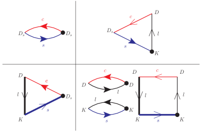
Figure 2: The quark line diagrams computed on the lattice. The charm, strange and light quarks are indicated by red, blue and black lines, respectively. Stochastic propagators are represented by lines with filled arrows and sequential stochastic propagators by two successive lines of the same width with open arrows. Time propagation is from right to left. The black dots indicate the stochastic source position. Note that the triangular diagrams are accompanied by a factor of 2 in Eq. (8) and the $DK\to DK$ diagrams are accompanied by a factor of 4 and 2 for the box and the product of $D$ and $K$ two-point functions, respectively, due to the summation over the light quark flavour, see Table 2.

The Wick contractions arising from Eq. (8) are shown in Fig. 2. These quark line diagrams are evaluated using spin and colour diluted complex $\mathbb{Z}_{2}$ stochastic sources with the one-end trick Foster and Michael (1999); McNeile and Michael (2003), following Refs. Aoki et al. (2007, 2011); Bali et al. (2016). Evaluation of the $DK\to DK$ box diagram requires two sequential propagators involving a combination of light and charm ($lc$) quarks and strange and light quarks ($sl$), represented by the thin and thick lines with open arrows in the bottom right of Fig. 2, respectively. These sequential propagators are recycled in the determination of the triangular diagrams that are averaged to improve the signal. The other propagators required (see the lines with filled arrows in Fig. 2) are similarly recycled where possible.

The $sl$ sequential combination is the most computationally expensive due to the need to realise the sequential source on every sink timeslice $t$ (cf. Eq. (8)). For this reason we restrict $t/a\in\left[5,19\right]$, a region chosen such that the excited state contributions to the resulting correlation functions are not large and the statistical noise is still under control. This restriction affects the box diagram and the lower left triangular diagram in Fig. 2. The remaining diagrams are evaluated for all timeslices and the (anti-) periodic boundary conditions in the temporal direction of length $T$ enable averaging over the time regions $0<t<T/2$ and $T/2<t<T$.

Gauge noise was found to dominate the correlator matrix and only the minimum number of stochastic sources was employed per configuration. This corresponds to 12$\times$2, where the first factor is due to spin-colour dilution and the second one arises because two independent stochastic sources are required for the $DK\to DK$ diagram involving the product of the $D$ and $K$ two-point functions. Spin dilution is required in order to study both the $0^{+}$ and $1^{+}$ states efficiently with the one-end trick. Colour dilution does not provide any reduction in the stochastic noise for fixed computational cost, however, implementing this within our code turned out to be convenient.

In order to ensure that for both the scalar and axialvector meson sectors we can resolve at least the lowest three states, we construct the $D_{s}$ and $D^{\prime}_{s}$ operators (see Table 2) with multiple spatial extents and the $DK$ operators with a single spatial extent. Wuppertal smearing Güsken et al. (1989) with 3 dimensionally APE smoothed spatial links Falcioni et al. (1985); Albanese et al. (1987) was applied with the number of Wuppertal iterations ($n_{\rm itr}$) equal to 16, 60 and $180$ for $O_{D_{s}}$ interpolators shared between quark and antiquark, $n_{\rm itr}=16,60$ for $O_{D^{\prime}_{s}}$ and $n_{\rm itr}=180$ for $O_{DK}$ operators. These choices are illustrated for the $0^{+}$ state in Fig. 3, which displays the effective masses of the diagonal components of the correlator matrix. As expected, increasing $n_{\rm itr}$ significantly boosts the overlap with the lowest state, at the cost of an increase in the noise at larger times. Similar behaviour is observed for the $1^{+}$. The determination of the lowest energy levels from the correlator matrix via the variational approach is discussed in Section V.1, along with the impact of the operator basis chosen. We also extract the decay constants of the $D_{s0}^{*}(2317)$ and $D_{s1}(2460)$, as described in Section V.5. For this purpose we compute the diagrams in the upper row of Fig. 2 with smeared source interpolators and local $O_{D_{s}}$ and $O_{D^{\prime}_{s}}$ sink operators.

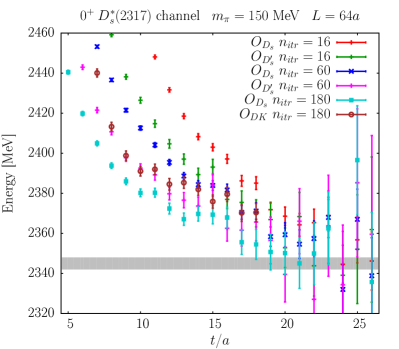
Figure 3: The effective masses for the diagonal elements of the $6\times 6$ correlator matrix for the $0^{+}$ channel for $m_{\pi}=150$ MeV and $L/a=64$. The operator basis for the matrix consists of three operators of type $O_{D_{s}}$ (see Table 2) with different levels of Wuppertal smearing iterations, two of type $O_{D^{\prime}_{s}}$ and one $O_{DK}$ interpolator. The grey band indicates the ground state energy extracted by solving the generalised eigenvalue problem Eqs. (4) and (5), see Section V for details.

In total a $6\times 6$ correlator matrix was realised at a computational cost of 14 charm quark, 3 strange quark and $N_{T}+3$ light quark inversions for each spin and colour component of the stochastic propagator (i.e. times 12 for the full cost) per configuration. We remark that in order to minimise the number of inversions, the smearing for each operator was split unevenly between the quark and antiquarks. The number of timeslices, $N_{T}=15$, for the light quark is due to the chosen range of the sink time mentioned above. The cost of these light quark inversions, equivalent to $N_{T}+3$ point-to-all propagators, represents the main overhead compared to a conventional analysis involving only quark-antiquark operators. For the restricted basis of operators considered here, the stochastic one end trick method we employed is substantially cheaper than the distillation technique used in Refs. Mohler et al. (2013); Lang et al. (2014) and enabled much larger lattice volumes to be realised. However, the latter approach becomes more attractive when considering a wider range of the meson spectrum involving several thresholds, see, for example, Refs. Moir et al. (2013); Prelovsek et al. (2015); Padmanath et al. (2015); Moir et al. (2016).

IV Theoretical background

In the following we briefly outline how energy levels measured on a finite lattice volume can be used to extract infinite volume information via a parametrisation of the $T$-matrix. Two approaches are considered. The first is based on Lüscher’s formalism and the effective range approximation, the second on a determination of the potential of the scattering particles in the chiral unitary approach.

IV.1 Lüscher’s method and the effective range approximation

For two relativistic particles with masses $m_{1}$ and $m_{2}$, scattering elastically in infinite volume, the $s$-wave $T$-matrix in the centre of momentum frame can be expressed as

$$T\left(s\right)=\frac{-8\pi\sqrt{s}}{p\cot\delta\left(p\right)-ip},$$ (9)

where $\sqrt{s}=E$ is the centre of momentum energy and $p$ is the modulus of the momentum of each particle,

$$p^{2}=\frac{\left(s-\left(m_{1}+m_{2}\right)^{2}\right)\left(s-\left(m_{1}-m_{2}\right)^{2}\right)}{4s}.$$ (10)

$\delta\left(p\right)$ is the $s$-wave phase shift and $p\cot\delta\left(p\right)$ is a real function of $p^{2}$ which can be expanded around the threshold $p^{2}=0$:

$$p\cot\delta\left(p\right)=\frac{1}{a_{0}}+\frac{1}{2}r_{0}p^{2}+\mathcal{O}\left(p^{4}\right).$$ (11)

The parameters $a_{0}$ and $r_{0}$ are the scattering length and the effective range, respectively, which, up to $\mathcal{O}\left(p^{4}\right)$, describe the low-energy scattering of the particles.

Above threshold, the $T$-matrix shows a unitarity cut which represents the continuous spectrum. Here, unitarity dictates that the imaginary part is given by, $\mbox{Im}\,T^{-1}\left(s\right)=\frac{p}{8\pi\sqrt{s}}$. Below threshold, $p=i|p|$ is imaginary and $T$ is real. If a bound state is present at $s=s_{B}\equiv m_{B}^{2}$ or $p=p_{B}$, it will appear as a pole of $T$ on the real axis:

$$p_{B}\cot\delta\left(p_{B}\right)=ip_{B}\equiv-|p_{B}|.$$ (12)

In the vicinity of the pole the $T$-matrix takes the form

$$T\left(s\right)\sim\frac{g^{2}}{s-s_{B}},$$ (13)

so that the coupling $g$ can be obtained through

$$g^{2}=\lim_{s\rightarrow s_{B}}T\left(s\right)\left(s-s_{B}\right)=\lim_{s\rightarrow s_{B}}\frac{-8\pi\sqrt{s}\left(s-s_{B}\right)}{p\cot\delta\left(p\right)-ip}.$$ (14)

At finite spatial volume, $L^{3}$, the energy levels and momenta are discretised and the cut of the $T$-matrix is replaced by poles at discrete values $s=s_{n}$:

$$\sqrt{s_{n}}=E_{n} = \sqrt{m_{1}^{2}+p_{n}^{2}}+\sqrt{m_{2}^{2}+p_{n}^{2}}$$ (15)

$$= \sqrt{m_{1}^{2}+k_{n}^{2}}+\sqrt{m_{2}^{2}+k_{n}^{2}}+\Delta E_{n},$$ (16)

where $\boldsymbol{k_{n}}=\frac{2\pi}{L}\boldsymbol{n}$, $\boldsymbol{p_{n}}=\frac{2\pi}{L}\boldsymbol{q_{n}}$, $\boldsymbol{n}\in\mathbb{Z}^{3}$ and $n=\sqrt{|\boldsymbol{n}|^{2}}=\sqrt{0},\sqrt{1},\sqrt{2},...$, while $\boldsymbol{q_{n}}$ are real valued vectors. The asymptotic two particle states in the infinite volume formalism are no longer free once placed in a finite box as the probability for them to be within the interaction range is finite. As $L$ increases, the interaction term $\Delta E_{n}$ tends to zero, $\boldsymbol{q_{n}}\rightarrow\boldsymbol{n}$ and $p^{2}_{n}\rightarrow k^{2}_{n}$. The position of the bound state pole $s_{B}$ is shifted to $s_{\widetilde{B}}$ at finite volume. We allow the index $n$ to assume an additional value $n=\widetilde{B}$ so that in Eqs. (15) and (16) $E_{\widetilde{B}}=m_{\widetilde{B}}$, $p_{\widetilde{B}}$ (imaginary) and $\Delta E_{\widetilde{B}}$ ($<0$) represent, respectively, the mass, binding momentum and binding energy of the bound state at finite volume. As $L\rightarrow\infty$, these quantities will tend to their infinite volume values $m_{B}$, $p_{B}$ and $\Delta E_{B}$.

Lüscher’s equation Lüscher (1991) (and its analytical continuation below threshold) relates the finite volume energy levels to the (infinite volume) partial wave phase shift $\delta\left(p\right)$. For $p=p_{n}$,

$$p\cot\delta\left(p\right)=\frac{2}{L\sqrt{\pi}}\mathcal{Z}_{00}\left(1;\frac{L^{2}}{4\pi^{2}}p^{2}\right),$$ (17)

for $s$-wave scattering, where $\mathcal{Z}_{00}$ is the (analytic continuation of the) generalised zeta-function. The latter has a simple exact expansion below threshold Sasaki and Yamazaki (2006), so that

$$p\cot\delta\left(p\right) = ip+\frac{1}{L}\sum_{n=1}^{\infty}\frac{\theta_{n}}{\sqrt{n}}e^{-\sqrt{n}|p|L}$$

$$= ip+\frac{1}{L}\left(6e^{-|p|L}+\frac{12}{\sqrt{2}}e^{-\sqrt{2}|p|L}+...\right),$$

where $\theta_{n}$ is the theta series of a simple cubic lattice. It is clear that as $L$ increases the summation term approaches zero and $p$ approaches the infinite volume binding momentum $p_{B}$ defined by Eq. (12). In principle, mixing with higher partial waves needs to be considered when determining the phase shift. However, these contributions are suppressed and for the energy range of interest in this study, it is reasonable to neglect them.

Covering energies (through varying the lattice extent $L$) that are below and above threshold, we compute $p\cot\delta\left(p\right)$ from Eq. (17) and perform the simple linear fit consistent with the effective range approximation Eq. (11) to determine $a_{0}$ and $r_{0}$. Then the bound state condition Eq. (12), which becomes

$$\frac{1}{a_{0}}-\frac{1}{2}r_{0}|p_{B}|^{2}=-|p_{B}|,$$ (19)

will provide the infinite volume binding momentum $p_{B}$ and thus the bound state mass $m_{B}$, using Eq. (15). Finally, the coupling can be evaluated within the same approximation by expanding the denominator of Eq. (14) around $s_{B}\equiv m_{B}^{2}$ and making use of Eq. (12), to arrive at

$$g^{2}=\frac{64\pi m_{B}p_{B}}{\left(1-r_{0}p_{B}\right)\left(1-\left(\frac{m_{1}^{2}-m_{2}^{2}}{m_{B}^{2}}\right)^{2}\right)}.$$ (20)

IV.2 Chiral unitary approach

Within the chiral unitary approach the $s$-wave $T$-matrix is expressed in terms of a (real) “potential” $V\left(s\right)$ for the scattering particles,

$$T\left(s\right)=\frac{1}{V^{-1}\left(s\right)-G\left(s\right)},$$ (21)

and a loop function $G\left(s\right)$ of two meson propagators,

$$G(s) = \int_{|\boldsymbol{k}|<\Lambda}\frac{d^{3}k}{\left(2\pi\right)^{3}}I\left(s,\boldsymbol{k}\right),$$ (22)

with

$$I\left(s,\boldsymbol{k}\right) = \frac{1}{2\omega_{1}\left(\boldsymbol{k}\right)\omega_{2}\left(\boldsymbol{k}\right)}\frac{\omega_{1}\left(\boldsymbol{k}\right)+\omega_{2}\left(\boldsymbol{k}\right)}{s-\left(\omega_{1}\left(\boldsymbol{k}\right)+\omega_{2}\left(\boldsymbol{k}\right)\right)^{2}}$$ (23)

and $\omega_{1/2}\left(\boldsymbol{k}\right)=\sqrt{m_{1/2}^{2}+\boldsymbol{k}^{2}}$. The integral is divergent and can be regularised by imposing a cut-off $\Lambda$ on the magnitude of $\boldsymbol{k}$. Alternatively, one can perform dimensional regularisation and introduce a subtraction constant, $\alpha(\mu)$, for a renormalisation scale $\mu$:

$$G\left(s\right) = \frac{1}{16\pi^{2}}\left[\alpha\left(\mu\right)+\log\frac{m_{1}m_{2}}{\mu^{2}}+\right.$$ (24)

$$\hskip 71.13188pt\left.\frac{\delta m}{2s}\log\frac{m_{2}^{2}}{m_{1}^{2}}+\frac{p}{\sqrt{s}}l\left(s\right)\right]$$

and

$$l\left(s\right) = +\log\left(2\sqrt{s}p+s+\delta m\right)+\log\left(2\sqrt{s}p+s-\delta m\right)$$

$$-\log\left(2\sqrt{s}p-s+\delta m\right)-\log\left(2\sqrt{s}p-s-\delta m\right),$$

where $\delta m=m_{2}^{2}-m_{1}^{2}$ and $p$ is given by Eq. (10).

With knowledge of the potential, the bound state mass, as a pole in the $T$-matrix, can be obtained by imposing the condition

$$V\left(s_{B}\right)G\left(s_{B}\right)=1,$$ (26)

while in the vicinity of the pole one can combine the parametrisation of Eq. (21) with Eq. (13) to derive the sum rule

$$\underbrace{g^{2}\frac{\partial V^{-1}}{\partial s}}_{Z}+\underbrace{g^{2}\left(-\frac{\partial G}{\partial s}\right)}_{1-Z}=1.$$ (27)

We remark that in weakly coupled quantum mechanics the potential $V$ can be interpreted as a perturbation to a hypothetical, non-interacting Hamiltonian $H_{0}$. Then $Z$ is the probability of the bound state to correspond to the one-particle sector of $H_{0}$ while $1-Z$ represents the probability that it is made up of more than one free particle, e.g., the $D$ and the $K$. This is known as Weinberg’s compositeness condition Weinberg (1965). For detailed discussions of the interpretation of this quantity within the present context see, for example, Refs. Baru et al. (2004); Gamermann et al. (2010); Hyodo (2013). However, it is not clear how meaningful this notion is for a strongly interacting quantum field theory. The nature of resonances in elastic scattering with a nearby $s$-wave threshold was earlier discussed in Refs. Morgan (1992); Morgan and Pennington (1993).

Note that the bound state mass, coupling and “compositeness” are independent of the choice of subtraction constant in Eq. (24) (or equivalently $\Lambda$ in Eq. (22)) since a change in $\alpha(\mu)$ is compensated for by a change in the potential such that physical quantities remain unaffected.

Expressions for the (scalar) potential for $K$ and $D$ meson scattering can be derived within heavy meson chiral perturbation theory Kolomeitsev and Lutz (2004); Hofmann and Lutz (2004); Guo et al. (2006); Gamermann et al. (2007); Guo et al. (2008, 2009); Cleven et al. (2011); Yao et al. (2015); Guo et al. (2015) (HMChPT). At leading order Kolomeitsev and Lutz (2004),

$$V\left(s\right)=\frac{1}{4F_{\pi}^{2}}\left[-3s+\frac{\left(m_{D}^{2}-m_{K}^{2}\right)^{2}}{s}+2\left(m_{D}^{2}+m_{K}^{2}\right)\right],$$ (28)

where $F_{\pi}$ is the pion decay constant with the normalisation corresponding to the experimental value of 92 MeV. However, the potential can also be extracted using the energy spectrum determined on the lattice. Neglecting finite volume effects on the potential that are exponentially suppressed, the $T$-matrix for a spatial extent $L$ reads

$$\widetilde{T}\left(s,L\right)=\frac{1}{V^{-1}\left(s\right)-\widetilde{G}\left(s,L\right)}.$$ (29)

The finite volume loop function is normally expressed as the sum of the infinite volume function (given by Eq. (24)) and a correction term $\Delta G\left(s,L\right)$,

$$\widetilde{G}\left(s,L\right) = G\left(s\right)+\Delta G\left(s,L\right),$$ (30)

where,

$$\Delta G\left(s,L\right) =$$ (31)

$$\lim_{\Lambda\rightarrow\infty}\left(\frac{1}{L^{3}}\sum_{\boldsymbol{k}}^{|\boldsymbol{k}|<\Lambda}-\int_{|\boldsymbol{k}|<\Lambda}\frac{d^{3}k}{\left(2\pi\right)^{3}}\right)I\left(s,\boldsymbol{k}\right).$$

The discrete sum is over the lattice momenta $\boldsymbol{k}=\frac{2\pi}{L}\boldsymbol{n},\quad\boldsymbol{n}\in\mathbb{Z}^{3}$. The lattice energy levels (squared), $s_{n}=s_{n}\left(L\right)$ in Eq. (15), correspond to poles of $\widetilde{T}$. Thus, the bound state condition

$$V^{-1}\left(s_{n}\right)=\widetilde{G}\left(s_{n},L\right)$$ (32)

allows us to probe the potential by evaluating $\widetilde{G}\left(s_{n},L\right)$ for each $s_{n}\left(L\right)$. Fitting the potential with a modelling function (see Section V.3), the bound state mass can be accessed by imposing Eq. (26) and the coupling and compositeness via Eq. (27).

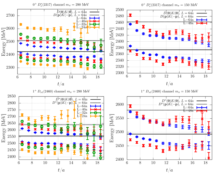
Figure 4: The effective masses of the lowest two eigenvalues for the $0^{+}$ (top) and $1^{+}$ (bottom) sectors on ensembles with $m_{\pi}=290$ MeV (left) and 150 MeV (right). The horizontal lines represent the lowest two free scattering states determined for the largest spatial volume at each pion mass, where for the second level corresponding to $D(\boldsymbol{p})K(-\boldsymbol{p})$, the spatial momentum $|\boldsymbol{p}|=2\pi/L$. A $4\times 4$ correlator matrix is employed in all the cases, consisting of the $O_{D^{(\prime)}_{s}}$ operators with three different smearing levels and the $O_{DK}$ operator with one smearing level (see Section III). The energies of the third eigenvalues lie much higher.

The infinite volume $T$-matrix can also be reconstructed:

$$T\left(s_{n}\right)=\frac{1}{\Delta G\left(s_{n},L\right)}.$$ (33)

This is independent of the regulator used. Note that when extracting the phase shift using Eq. (9) an explicit form for the potential does not have to be introduced. Indeed, as shown in Ref. Doring et al. (2011), this is a more general approach than Lüscher’s, as small volume contributions are kept. However, in this work, we find these additional contributions to be negligible.

V Results

The matrix of correlators in Eq. (8) is constructed for each ensemble and the variational method applied. The extraction of the (finite volume) spectra from the resulting eigenvalues is presented in the next subsection. The phase shifts and infinite volume information, including the masses and couplings, derived from the spectra via Lüscher’s formalism are presented in Section V.2, followed by a complementary analysis via the chiral unitary approach in Section V.3. Our results for the low lying $D_{s}$ spectrum are given in Section V.4. In addition, we determine the scalar and vector decay constants of the $D_{s0}^{*}(2317)$ and the axialvector and tensor decay constants of the $D_{s1}^{*}(2460)$ in Section V.5.

V.1 Energies

For each channel of interest the operator basis for constructing the correlator matrix in Eq. (8) is varied in order to determine the influence of each interpolator on the energy spectrum and to realise the best signals possible. Considering the $0^{+}$ channel first, a basis of four operators consisting of $O_{D_{s}}$ with all three smearing levels and $O_{DK}$ with a single smearing level (see Section III and Table 2) proved sufficient for extracting the lowest two energies corresponding to the bound state and the scattering state, as demonstrated below. The quality of the signal achieved is illustrated in Fig. 4, which displays the effective masses,

$$E_{n}\left(t+a/2,t_{0}\right)=\log\frac{\lambda_{n}\left(t,t_{0}\right)}{\lambda_{n}\left(t+a,t_{0}\right)},$$ (34)

for the two levels on all ensembles in the time range $t/a\in\left[6,19\right]$ where $t>t_{0}$ and $t_{0}$ is set to $5a$. Utilising higher values of $t_{0}$ gave consistent results. As discussed in Section III, the range of $t$ is smaller than the lattice temporal extent as the computational cost in terms of the number of light quark inversions for some elements of the correlator matrix is roughly proportional to the number of sink timeslices.

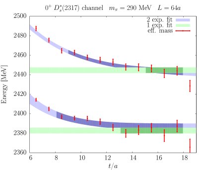
Figure 5: The effective masses of the lowest two eigenvalues in the $0^{+}$ channel compared to the results from one and two exponential fits indicated by the green and blue bands, respectively, for the $m_{\pi}=290$ MeV, $L/a=64$ ensemble. The fitting ranges in each case are marked by the darker colours. The eigenvalues are generated from a $4\times 4$ correlator matrix as in Fig. 3.

Figure 4 shows that unwanted contributions to the eigenvalues from other (higher) states die away around timeslices 12–14 corresponding to the physical distances 0.8–1.0 fm. As the spatial volume is increased the energy of the lowest state increases and the next level decreases, tending towards the non-interacting threshold. This behaviour is compatible with that of a bound state (the $D_{s0}^{*}(2317)$) that couples to the $DK$ threshold and a scattering state. The final results for the energies are extracted by fitting the eigenvalues within a chosen time window. The end point for the fit ($t_{\rm max}$) needs to be fixed with care due to the short physical time extent of the lattices, corresponding to 3.4 fm for $L=24a$ and 4.5 fm for $L>24a$. For (anti) periodic boundary conditions in the temporal direction, there are additional contributions to the spectral decomposition of $C_{ij}(t)$ in Eq. (3). These include terms arising from backward propagation in time of the form $Z_{ki}Z_{kj}^{\dagger}e^{-E_{k}(T-t)}$, which can be neglected for $t<T/2$ in our analysis due to the size of $E_{k}$ and $T$. However, there are also so-called “thermal” contributions involving two particles, one travelling forward in time, the other propagating backward. These particles can be a $D$ and a $K$ meson, respectively, leading to the contribution,

$$\langle D|O_{i}|K\rangle\langle K|O^{\dagger}_{j}|D\rangle e^{-(T-t)m_{K}}e^{-m_{D}t},$$ (35)

which may be significant around $t=T/2$, making the extraction of the $D_{s}$ meson and scattering energies less straightforward. If the overlaps in Eq. (35) are of the same order of magnitude as the leading forward propagating overlaps in Eq. (3) then at $t=19a$ ($17a$) for $T/a=64$ (48) these contributions are of the order of the statistical errors in the correlator matrix, decreasing rapidly for smaller $t$. In the case of two degenerate particles, Eq. (35) reduces to a constant term which can be removed by taking finite differences, see Ref. Helmes et al. (2015). Here we choose $t_{\rm max}<19a$ ($17a$) for $T/a=64$ (48) to avoid any significant contribution from thermal states.

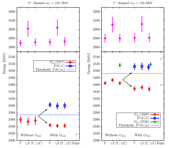
Figure 6: Lowest energy levels of the $0^{+}$ (left) and $1^{+}$ (right) channels extracted from fits to the eigenvalues for different operator bases for the $m_{\pi}=150$ MeV, $L/a=64$ ensemble. The basis is indicated at the bottom of the figure, where $\Gamma$ refers to the spin structure of the quark-antiquark interpolators, $\bar{s}\Gamma c$ (see Table 2) with $\Gamma=\mathbb{1}$ and $\gamma_{i}\gamma_{5}$ for the $0^{+}$ and $1^{+}$ mesons, respectively. All smearing levels are utilised for each operator (see Section III), such that for the $1^{+}$ states when including the $D^{*}K$ interpolators, the results labelled with “$\Gamma$” are determined from a $4\times 4$ correlator matrix, while $(\Gamma,\gamma_{t}\Gamma)$ refers to a $6\times 6$ matrix. The exception is the $(\Gamma,\gamma_{t}\Gamma)$ combination (with and without the $DK$ operators) for the scalar channel for which only the $\gamma_{t}\Gamma$ operator with the largest smearing is employed. The non-interacting $DK$ and $D^{*}K$ thresholds for this ensemble are also shown as the dashed blue lines. The black arrows emphasise the fact that the lowest energy extracted without the two meson operators present is contaminated by contributions from the finite volume “scattering” state $D^{(*)}K(L)$ and this level and the ground state are only isolated once the $DK$ interpolators are included.

Both single and double exponential fits were performed to each eigenvalue, giving compatible results as demonstrated in Fig. 5 for the $m_{\pi}=290$ MeV, $L/a=64$ ensemble. The starting point for the fit window ($t_{\rm min}$) was set requiring that the correlated $\chi^{2}/d.o.f.$ is less than 2 and that larger values for $t_{\rm min}$ give consistent results within errors. The energies extracted depend on the operator basis of the correlator matrix as displayed in Fig. 6. In particular, a basis comprised of only $O_{D_{s}}$ interpolators gives the first energy level around 2360 MeV with the next state lying much higher, above 2800 MeV. The $O_{D^{\prime}_{s}}$ operators give the same spectrum but with larger statistical errors for the lowest level, also when combined with $O_{D_{s}}$.

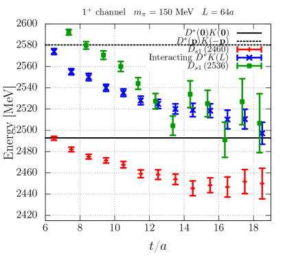
Figure 7: The effective masses of the first three eigenvalues in the axialvector channel for a $6\times 6$ correlator matrix involving a basis of $O_{D_{s}}$, $O_{D^{\prime}_{s}}$ and $O_{DK}$ operators for the $m_{\pi}=150$ MeV, $L/a=64$ ensemble. The horizontal lines represent the lowest two free scattering states, where for the second level corresponding to $D(\boldsymbol{p})K(-\boldsymbol{p})$, the spatial momentum $|\boldsymbol{p}|=2\pi/L$.

The first (finite volume) scattering level is only resolved when including the $DK$ operators, with the ground state extracted being shifted approximately 15 MeV lower. This suggests that our choice of two quark interpolators has overlap with both of the two (closely lying) lowest levels and that the ground state is not isolated within the time window realised $t<19a$ or 1.3 fm if the two meson operators are omitted. We note that similar observations using two and four quark operator bases constructed via the distillation approach were made in Refs. Mohler et al. (2013); Lang et al. (2014), although in general a different basis, for example, in terms of the spin structure or spatial extension, can lead to different behaviour. As seen in the figure, the best signal is obtained from a $4\times 4$ correlator matrix with all three $O_{D_{s}}$ operators and the $DK$ interpolator. This turned out to be the case for all ensembles. The final results for the lowest two levels are summarised in Table 3.

Given the difficulty in extracting the spectrum of closely lying levels, we remark that the second non-interacting threshold arising from a $D$ and $K$ meson with opposite momentum, $|\boldsymbol{p}|=2\pi/L$, lies approximately $85$ MeV above the first (with $|\boldsymbol{p}|=0$) for the largest spatial volumes, see Fig. 4. The corresponding finite volume scattering levels will be similarly close. The inclusion of operators of the form $D\left(\boldsymbol{p}\right)K\left(-\boldsymbol{p}\right)$ (omitted in our analysis) would help determine whether the energy of the lowest scattering level is reliably determined in our analysis. Any contamination from higher states is likely to be a small effect, becoming even less significant for the smaller spatial volumes, as suggested by the fact that the energy difference between the lowest two non-interacting thresholds becomes much larger, rising to 494 MeV for $L/a=24$.

Table 3: Results in MeV for the lowest energy levels extracted in the scalar and axialvector channels. The error given is statistical derived from jackknife resampling for the chosen fit window. Changing the window and/or type of fit (including one or two exponentials), for reasonable $\chi^{2}/d.o.f$, gives a variation in the central values within $\pm 1\sigma$ of the statistical errors. Note that in the axialvector case we extract two states (in addition to the scattering level) and both are labelled $D_{s1}$.

	$J^{P}=0^{+}$		$J^{P}=1^{+}$
$L/a$	$D_{s0}^{*}$	$DK$	$D_{s1}$	$D^{*}K$	$D_{s1}$
$m_{\pi}=290$ MeV
$\>24\>$	$\>2318(5)\>$	$\>2594(13)\>$	$2435(6)$	$\>2691(16)\>$	$2549(14)$
$32$	$2352(5)$	$2529(5)$	$2469(6)$	$\>2621(14)\>$	$2540(17)$
$40$	$2362(4)$	$2485(6)$	$2477(8)$	$2602(6)$	$2574(11)$
$64$	$2382(3)$	$2440(5)$	$2496(4)$	$2570(3)$	$2552(5)$
$m_{\pi}=150$ MeV
$48$	$2332(5)$	$2417(6)$	$2440(4)$	$2535(4)$	$2533(6)$
$64$	$2344(4)$	$2402(6)$	$2449(5)$	$2513(8)$	$2519(5)$

The analysis of the axialvector channel proceeds in a similar way. In this case, in addition to the bound state $D_{s1}(2460)$ and scattering level one expects a resonance, the $D_{s1}(2536)$, just above threshold. As Figs. 4 and 7 show, an $O_{D_{s}}$, $O_{DK}$ basis resolves two closely lying levels, while the third is only isolated when $O_{D^{\prime}_{s}}$ interpolators are included. Varying the basis for the correlator matrix, we identify the scattering level to be the one which is only resolved when the $D^{*}K$ interpolators are included (like for the scalar channel, see Fig. 6 and that tends towards the non-interacting threshold as the spatial volume increases. The ground state is also only cleanly extracted when the $D^{*}K$ interpolators are included, while for the third level the basis must include both $O_{D_{s}}$ and $O_{D^{\prime}_{s}}$. The final results for the axialvector channel on all ensembles are detailed in Table 3. In contrast to the ground state, the third level that we identify as the $D_{s1}(2536)$ is insensitive to the spatial volume suggesting only a small coupling to the $D^{*}K$ threshold. This state lies below the threshold for the ensembles with $m_{\pi}=290$ MeV, rising to slightly above but consistent with the scattering level for $m_{\pi}=150$ MeV.

V.2 Phase shifts, scattering lengths and infinite volume energies

The energy levels presented in the previous subsection are consistent with the expected spectrum. However, the nature of the physical states and the infinite volume information — phase shifts, energies and scattering lengths etc. — should be accessed via Lüscher’s relation. For each energy level we first determine the corresponding momenta of two particles undergoing elastic scattering via Eq. (15). The continuum dispersion relation is assumed to apply for the relevant $D^{(*)}$ and $K$ mesons, although, discretisation effects can lead to deviations at finite lattice spacing. Figure 8 demonstrates that the continuum dispersion relation reproduces the finite momentum $D$ and $K$ meson energies to within the $0.4\%$ and $0.7\%$ statistical errors, respectively, for the range of momenta of interest in this study: $p<400$ MeV for the example of $m_{\pi}=150$ MeV and $L/a=64$. Similar behaviour is seen for the other ensembles and also for the $D^{*}$ meson.

The rest masses of the scattering mesons are required as input in Eq. (15). The values in Table 1 indicate a mild dependence on the volume, although this is only statistically significant ($>3\sigma$) for $m_{K}$ between $L=24a$ and larger spatial extents for the $m_{\pi}=290$ MeV ensembles. We prefer to use the masses from $L=64a$ as estimates of the infinite volume values throughout because we are relating the spectra to scattering amplitudes in this limit. Systematics due to finite $L$ are discussed below.

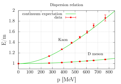
Figure 8: The dispersion relation for the $K$ and $D$ mesons for the $m_{\pi}=150$ MeV, $L/a=64$ ensemble from a subset of configurations, $N_{\rm conf}=600$.

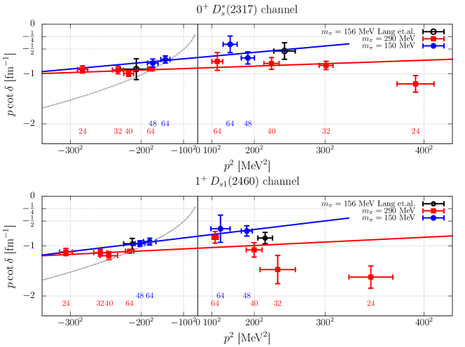
Figure 9: The combination $p\cot\delta$ as a function of $p^{2}$ for the $0^{+}$ (top) and $1^{+}$ (bottom) sectors. The threshold $p^{2}=0$ separates the bound state (left) and scattering state (right) regions. Linear fits to the data excluding the $L=24a$ results are shown as red and blue lines while the dashed curve indicates $ip=-\sqrt{-p^{2}}$. The inverse scattering length $1/a_{0}$ can be read off from the intersection with the threshold. The results of Lang et al. Lang et al. (2014) from an ensemble with near physical pion mass are shown for comparison.

For the ground state and scattering level in the scalar and axialvector channels, the phase shifts are extracted in the combination $p\cot\delta$ utilising Eq. (17). The third state in the axialvector channel is treated separately due to the lack of volume dependence, indicating a small coupling to the $D^{*}K$ threshold. This is discussed further in Section V.4. Figure 9 presents the results as a function of $p^{2}$ for all ensembles. The intersection of the data with the curve representing $ip=-\sqrt{-p^{2}}$ indicates the position of the pole in the $T$-matrix in infinite volume (according to Eqs. (9) and (IV.1)). As seen in the figure, the results from the largest ensembles for both channels and pion masses lie very close to the intersection.

Within the effective range approximation of Eq. (11), $p\cot\delta$ is linearly dependent on $p^{2}$. The data are reasonably consistent with this expectation apart from the results of the smallest spatial volume, $L=24a\approx 1.7$ fm at $m_{\pi}=290$ MeV. This may be due to the breakdown of the approximation and/or the presence of finite volume effects that are exponentially suppressed with $Lm_{\pi}$, not taken into account in Lüscher’s formalism. Performing a linear fit excluding the $L=24a$ data, we obtain the scattering length $a_{0}$ and the effective range $r_{0}$. The infinite-volume binding momentum, $p_{B}$, can then be accessed via Eq. (19) and subsequently the bound state mass and the coupling $g$ through Eqs. (15) and (20), respectively. Note that in terms of $Lm_{\pi}$ the $L=48a$ lattice at $m_{\pi}=150$ MeV is similar in size, however, in this case $p^{2}$ is closer to the threshold and to leading order in ChPT the exponential corrections are additionally suppressed by a factor of $m_{\pi}^{2}$.

Table 4: Scattering length $a_{0}$, effective range $r_{0}$, infinite-volume binding momentum $|p_{B}|$, threshold splitting $\Delta m$, infinite volume mass $m_{D_{s}}$ and coupling $g$ for the scalar and axialvector channels for the $m_{\pi}=290$ MeV and $m_{\pi}=150$ MeV ensembles. The first error is statistical while the second indicates the shift in the central value if the analysis is repeated using only the $L/a=64$ data for $m_{\pi}=150$ MeV and $L/a=40$ and $64$ data for $m_{\pi}=290$ MeV. The physical value of $m_{D_{s}}$ and $\Delta m=m_{D}+m_{K}-m_{D_{s}}$ for the QCD theory are also given (labelled as “Expt”). See Section II for details of how isospin breaking and electromagnetic effects are taken into account.

	$0^{+}$ channel			$1^{+}$ channel
	$m_{\pi}=290$ MeV	$m_{\pi}=150$ MeV	Expt.	$m_{\pi}=290$ MeV	$m_{\pi}=150$ MeV	Expt.
$a_{0}$ [fm]	$-1.13(0.04)(+0.05)$	$-1.49(0.13)(-0.30)$		$-0.96(0.05)(-0.04)$	$-1.24(0.09)(-0.12)$
$r_{0}$ [fm]	$0.08(0.03)(+0.08)$	$0.20(0.09)(+0.31)$		$0.11(0.06)(+0.08)$	$0.27(0.07)(+0.13)$
$|p_{B}|$ [MeV]	$180(6)(0)$	$142(11)(-9)$		$219(7)(0)$	$180(11)(-3)$
$\Delta m$ [MeV]	$40(3)(0)$	$26(4)(-3)$	$42.6(0.7)(2.0)$	$59(4)(0)$	$42(5)(-2)$	$42.9(0.7)(2.0)$
$\>m_{D_{s}}\>$ [MeV]	$\>2384(2)(-1)\>$	$\>2348(4)(+6)\>$	$\>2317.7(0.6)(2.0)\>$	$\>2497(4)(-1)\>$	$\>2451(4)(+1)\>$	$\>2459.5(0.6)(2.0)\>$
$g$ [GeV]	$11.9(0.3)(+0.5)$	$11.0(0.6)(+1.2)$		$14.2(0.6)(+0.7)$	$13.8(0.7)(+1.1)$

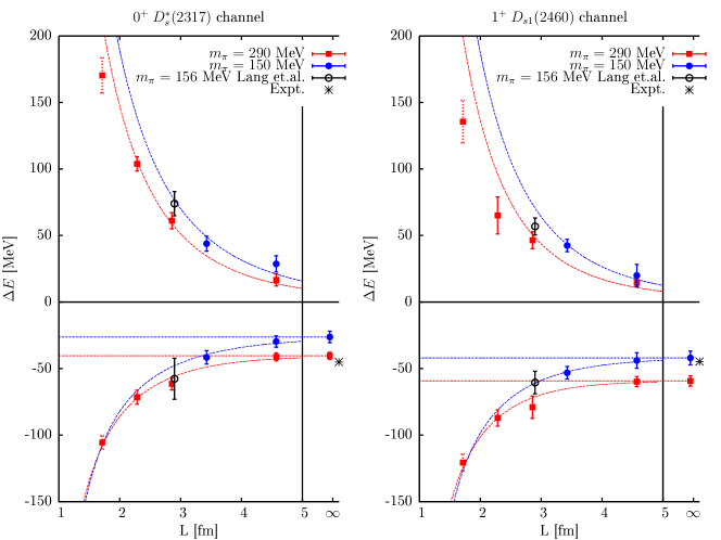
Figure 10: The splittings of the two lowest states with the non-interacting threshold for the scalar and axialvector channels for $m_{\pi}=290$ MeV and 150 MeV. Displayed as dashed lines is the dependence on $L$ derived using the effective range approximation for $p\cot\delta$ and Eqs. (16) and (17) with the central values for $a_{0}$ and $r_{0}$ of Table 3. The infinite-volume splitting, also given in Table 3, is shown (statistical errors only) along with the corrected experimental values. The horizontal lines indicate the infinite volume binding energy of the states for each pion mass. In addition, the results of Ref. Lang et al. (2014) (Lang et al.) are included for comparison.

The results for these quantities are compiled in Table 4. The first error given corresponds to the statistical uncertainty while the second is an estimate of possible residual finite volume effects due to the exponentially suppressed terms mentioned above. This estimate is computed by performing the fits to $p\cot\delta$ excluding the data from the smallest spatial extent. This means using only the $L/a=64$ results, i.e. two data points, at $m_{\pi}=150$ MeV and the $L/a=40$ and $64$ results at $m_{\pi}=290$ MeV. The shifts in the central values for most quantities are around one to two statistical standard deviations or less of the original results. Larger shifts are found for $a_{0}$ and $r_{0}$, in particular, for the lightest ensemble, however, the results are still consistent given the larger statistical errors for the reduced fits.

In both channels the scattering length is negative, compatible with the existence of a bound state. The masses of these states depend on the pion mass, decreasing by 36(4) MeV and 46(5) MeV between $m_{\pi}=290$ and 150 MeV for the $0^{+}$ and $1^{+}$, respectively. The errors indicated are due to statistics only. Similarly, the second $1^{+}$ level also decreases by 33(7) MeV (see the $L=64a$ data in Table 3). These shifts are much larger than for the lower lying pseudoscalar and vector $D_{s}$ meson masses which decrease by 3 MeV (from 1980(1) MeV at $m_{\pi}=290$ MeV to 1977(1) at $m_{\pi}=150$ MeV) and 7 MeV (from 2101(1) MeV to 2094(1) MeV), respectively, hinting that the $0^{+}$ and $1^{+}$ states may have a more complicated internal structure. The (lower) axialvector level for the smallest pion mass is reasonably consistent with experiment, while the scalar lies somewhat high. This mismatch is likely to be due to discretisation effects and is discussed further in Section V.4. As expected, considering Fig. 9, the results for the largest spatial extent at each pion mass in Table 3 are consistent with the infinite volume values.

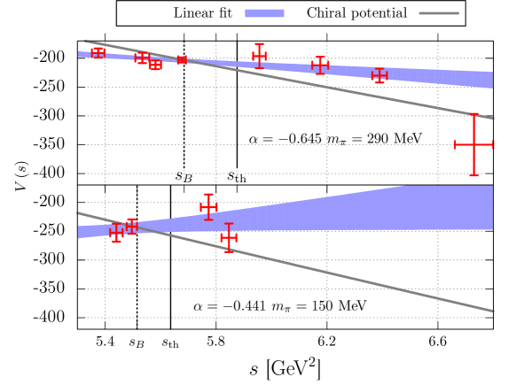
Figure 11: The potential of the scattering $D$ and $K$ meson in the scalar channel as a function of the square of the energy in the centre of momentum frame. The subtraction constant $\alpha(\mu)$ of Eq. (24), utilised for each pion mass, is fixed such that the potential from HMChPT (Eq. (28), also shown as a grey line) reproduces the lattice bound state mass for the $L=64a$ ensembles. The renormalisation scale $\mu$ is set to $m_{D}$. Linear fits to the lattice data are shown with one sigma error bars, while vertical lines indicate the squared energy of the bound state ($s_{B}$) and also the non-interacting threshold ($s_{\rm th}$). Note that the potential is defined to be dimensionless.

A comparison can be made with the study of Ref. Lang et al. (2014), which also includes a near physical pion mass ensemble with $m_{\pi}=156$ MeV, although the lattice spacing is coarser, $a=0.09$ fm, and the spatial extent is smaller, $L=2.9$ fm. As shown in Fig. 9, the results for $p\cot\delta$ are consistent for both the scalar and axialvector cases, in particular, when comparing with the linear fit to our data at the larger $|p^{2}|$ values realised in Ref. Lang et al. (2014). Not surprisingly, the scattering lengths and effective ranges they extract are similar to ours with $a_{0}=-1.33(20)$ fm and $r_{0}=0.27(17)$ fm for the scalar and $a_{0}=-1.11(11)$ fm and $r_{0}=0.10(10)$ fm for the axialvector. The coupling for this simulation was evaluated in a separate study Martínez Torres et al. (2015) with the results, $g=12.6(1.5)$ GeV and $12.6(7)$ GeV for the scalar and axialvector channels, respectively, in reasonable agreement with our values in Table 4. This study focused on an analysis of the Mohler et al. Mohler et al. (2013) and Lang et al. Lang et al. (2014) data within the chiral unitary approach Martínez Torres et al. (2015), discussed in the next subsection.

Another quantity of interest is the binding energy, i.e. the splitting of the bound state with respect to the (non-interacting) threshold. This is computed at finite $L$ as well as in the infinite volume limit. The values for the latter (denoted $\Delta m$) are given in Table 3 while the dependence on $L$ is displayed in Fig. 10 together with the results of Ref. Lang et al. (2014) for $m_{\pi}=156$ MeV for comparison. Also included in the figure is the same splitting for the lowest scattering levels, which, as expected, tends to zero with increasing spatial extent. To guide the eye, we employ the effective range approximation together with the fits to $p\cot\delta$ shown in Fig. 9 to derive the dependence on $L$ via Eqs. (16) and (17), indicated by the dashed lines. The consistency found with the data is a reflection of the agreement seen in Fig. 9. For $m_{\pi}=150$ MeV, $\Delta m$ in the axialvector channel is compatible with the physical values, while we undershoot by 17 MeV for the scalar case. Taking the spin-average of the two channels to minimise lattice spacing effects (see Section V.4) gives a splitting of $\Delta\overline{m}=38(4)$ MeV which is within 2$\sigma$ of $43(7)(2.0)$ MeV for the QCD theory. We remark that the scalar and axialvector states are more strongly bound for heavier pion mass.

V.3 Potential

We now consider the chiral unitary approach as an alternative method for extracting the bound state mass and coupling. The first step is to compute the potential through Eq. (29) for each energy level squared $s_{n}$. We employ dimensional regularisation for the continuum loop function $G(s)$ for a range of $\alpha(\mu)$ from $-0.4$ to $-2.2$ with the renormalisation scale fixed to $\mu=m_{D}$ and $m_{D^{*}}$ for the scalar and axialvector cases, respectively. This range is chosen to encompass values consistent with imposing a cut-off of $k_{\rm max}\sim\sqrt{\Lambda_{\chi}^{2}-m_{K}^{2}}\sim 0.87$ GeV in Eq. (22), where the chiral symmetry breaking scale $\Lambda_{\chi}\sim 1$ GeV. In particular, in Ref. Guo et al. (2006) $G(s)$, evaluated by imposing $k_{\rm max}=0.8-0.9$ GeV, was found to be equivalent to $\alpha\sim-0.6$. The results for the scalar potential are displayed in Fig. 11 for the values of $\alpha$ which match $V(s)$ for the $L=64a$ ensembles to the HMChPT potential Eq. (28). In the axialvector case the potential shows a similar dependence on the squared energy.

Table 5: The bound state mass, the coupling and the compositeness $1-Z$ for the scalar and axialvector channels extracted using the chiral unitary approach via linear fits to the potential for a range of values of the subtraction constant $\alpha$ (see the text). The first error is statistical while the second indicates the shift in the central value if the analysis is repeated using only the $L/a=64$ data for $m_{\pi}=150$ MeV and the $L/a=40$ and $64$ data for $m_{\pi}=290$ MeV.

	Scalar
	$m_{\pi}=290$ MeV			$m_{\pi}=150$ MeV
$\alpha$	-0.4	-1.4	-2.2	-0.4	-1.4	-2.2
$\>m_{D_{s}}\>$ [MeV]	$2384(3)(0)$	$2384(2)(0)$	$2384(2)(0)$	$2348(5)(+3)$	$2348(4)(+3)$	$2348(4)(+3)$
$g$ [GeV]	$11.7(0.3)(+0.7)$	$11.7(0.3)(+0.7)$	$11.8(0.3)(+0.7)$	$11.2(0.6)(+1.0)$	$11.1(0.6)(+1.0)$	$11.1(0.6)(+1.1)$
$1-Z$	$0.90(0.04)(+0.10)$	$0.90(0.03)(+0.10)$	$0.90(0.03)(+0.10)$	$1.08(0.08)(+0.23)$	$1.04(0.08)(+0.30)$	$1.04(0.08)(+0.31)$
	Axialvector
	$m_{\pi}=290$ MeV			$m_{\pi}=150$ MeV
$\alpha$	-0.4	-1.4	-2.2	-0.4	-1.4	-2.2
$\>m_{D_{s}}\>$ [MeV]	$2500(4)(-3)$	$2498(4)(-1)$	$2497(3)(-1)$	$2451(4)(+1)$	$2451(4)(+1)$	$2451(4)(+1)$
$g$ [GeV]	$14.3(0.5)(+1.2)$	$14.1(0.5)(+1.0)$	$14.0(0.5)(+1.0)$	$13.8(0.6)(+0.6)$	$13.8(0.6)(+1.0)$	$13.8(0.6)(+1.0)$
$1-Z$	$1.00(0.08)(+0.14)$	$0.95(0.07)(+0.14)$	$0.94(0.07)(+0.13)$	$1.13(0.08)(+0.17)$	$1.14(0.09)(+0.19)$	$1.14(0.09)(+0.19)$

Table 6: Comparison of results for the scattering length, effective range, coupling and compositeness for the $D_{s0}^{*}(2317)$ and the $D_{s1}(2460)$ from the lattice and unitarised HMChPT. Note that the lattice results of this work and Mohler et al. Mohler et al. (2013) and Lang et al. Lang et al. (2014) were obtained using near physical pion masses, $m_{\pi}=150$ MeV and 156 MeV, respectively. The ^† symbol indicates that the coupling is given in Ref. Martínez Torres et al. (2015) where a re-analysis of the data from Refs. Mohler et al. (2013); Lang et al. (2014) was also performed within the effective range approximation. For the HMChPT studies we indicate if lattice and/or experimental input has been utilised, see the references for details. Liu et al. in Ref. Liu et al. (2013) perform a lattice study of $K\overline{D}$ at unphysical quark mass and use SU(3) flavour symmetry to relate the results to that for the $DK$ system.

	$a_{0}$ [fm]	$r_{0}$ [fm]	$g$ [GeV]	$1-Z$
Scalar
This work	-1.49(0.13)(-0.30)	0.20(0.09)(+0.31)	11.0(0.6)(+1.2)	1.04(0.08)(+0.30)
Refs. Mohler et al. (2013); Lang et al. (2014): LQCD	-1.33(20)	0.27(17)	12.6(1.5)†
Ref. Martínez Torres et al. (2015): HMChPT+LQCD Mohler et al. (2013); Lang et al. (2014)	-1.3(5)(1)	-0.1(3)(1)	11.3	0.72(13)(5)
Ref. Liu et al. (2013): LQCD+HMChPT	-0.86(3)			0.72-0.66
Ref. Guo et al. (2006): HMChPT+Expt			10.203
Ref. Yao et al. (2015): HMChPT+Expt+LQCD Liu et al. (2013); Mohler et al. (2013); Lang et al. (2014)	$-1.04^{+0.06}_{-0.03}$
Ref. Guo et al. (2015): HMChPT+Expt+LQCD Liu et al. (2013); Mohler et al. (2013); Lang et al. (2014)	$-0.89^{+0.06}_{-0.10}$
Ref. Albaladejo et al. (2016): HMChPT+Expt	$-0.95^{+0.15+0.08}_{-0.15-0.13}$			$0.70^{+4+4}_{-6-8}$
Axialvector
This work	-1.24(0.09)(-0.12)	0.27(0.07)(+0.13)	13.8(0.7)(+1.1)	1.14(0.09)(+0.19)
Refs. Mohler et al. (2013); Lang et al. (2014): LQCD	-1.11(11)	0.10(10)	12.6(7)†
Ref. Martínez Torres et al. (2015): HMChPT+LQCD Mohler et al. (2013); Lang et al. (2014)	-1.1(5)(2)	-0.2(3)(1)	14.2	0.57(21)(6)

The next step is to fit the potential with a reasonable functional form. A linear ansatz is the natural choice in the small region around threshold we are considering and is consistent with the data, apart from the smallest volume ensemble at $m_{\pi}=290$ MeV. For the latter, we may be observing finite volume effects, although there is also the possibility of the influence of the $D_{s}\eta$ threshold or Castillejo-Dalitz-Dyson poles Castillejo et al. (1956). Performing linear fits (omitting the $L=24a$ results) and utilising Eqs. (26) and (27) we obtain the bound state masses and couplings given in Table 5. These physical results are independent of the subtraction constant employed, as they should be, and are compatible with the values determined through Lüscher’s formalism and the effective range approximation. The two errors shown are, respectively, statistical and systematic, representing an estimate of finite volume effects, computed by performing a reduced fit in the same way as discussed in the previous subsection. Note that the phase shift extracted in this approach through Eqs. (32) and (9) is numerically very similar to the results of the previous subsection and hence the effective range and scattering length extracted are in agreement with the values in Table 4.

For comparison we also display the scalar potential from leading order HMChPT Kolomeitsev and Lutz (2004) in Fig. 11. We apply the values of $m_{D}$, $m_{K}$ and $F_{\pi}$ from the $L=64a$ ensemble for each pion mass. The pion decay constant, determined in Ref. Bali et al. (2015), is equal to 95.1(3) MeV at $m_{\pi}=290$ MeV and 85(1) MeV at $m_{\pi}=150$ MeV, indicating that we undershoot the experimental result. This may be due to discretisation effects at the present lattice spacing ($a=0.071$ fm). The value of $\alpha$ for each pion mass is chosen such that the bound state energy level for the largest ensemble is reproduced by the HMChPT potential. This matching is reflected in the figure by the potential intersecting the large ensemble results. One can see that for the short range of $s$ realised in the lattice data this potential is approximately linear. The slope is somewhat steeper than the lattice data suggests and the couplings derived from Eqs. (27) and (28), $g=10.7$ GeV and 9.8 GeV for $m_{\pi}=290$ MeV and 150 MeV, respectively (that are independent of the subtraction constant) are slightly lower compared to the results from our fits, cf. Table 5. If the phenomenological values for the masses and decay constant are utilised, the HMChPT potential gives $g=10.7$ GeV.

Details of the higher order HMChPT terms for the potential can be found in Refs. Hofmann and Lutz (2004); Guo et al. (2008, 2009); Cleven et al. (2011); Guo et al. (2015); Yao et al. (2015) and of other chiral models, for example, in Ref. Gamermann et al. (2007). These works also consider coupled channel effects. Table 6 compares recent results employing HMChPT with this study and that of Mohler et al. Mohler et al. (2013) and Lang et al. Lang et al. (2014), where most works determine the scattering length. In many cases some input from the lattice is taken and overall $a_{0}$ tends to be lower.

Regarding the compositeness of the bound state, we find a strong $DK$ component in the wave function with $1-Z\approx 1$ to within 2 sigma in the statistical errors for $m_{\pi}=150$ MeV for both the scalar and axialvector channels, with slightly lower values for the larger pion mass. A large systematic shift is encountered when trying to estimate finite volume effects, in particular, for $m_{\pi}=150$ MeV due to the limited number of data points available. These results are higher than those determined in a similar analysis of the Mohler et al. Mohler et al. (2013) and Lang et al. Lang et al. (2014) data at $m_{\pi}=156$ MeV. The authors of Ref. Martínez Torres et al. (2015) found $1-Z=0.72(13)(5)$ for the $0^{+}$ and 0.57(21)(6) for the $1^{+}$, although the errors are large.

Finally, HMChPT at leading order provides broadly similar values in the scalar case which increase with pion mass, with $1-Z=0.75$ and 0.81 for $m_{\pi}=290$ and 150 MeV, respectively (independent of $\alpha(\mu)$). This can be compared to $1-Z=0.71$ when imposing the physical values of $F_{\pi}$, $m_{K}$ and $m_{D}$. The HMChPT potential has also been employed to fit the experimental $DK$ invariant mass distributions of $B\to DDK$ and $B_{s}\to\pi DK$ decays, giving a prediction for $1-Z$ of $0.70^{+4+4}_{-6-8}$ Albaladejo et al. (2016). As already remarked below Eq. (27), the precise meaning of $Z$ in a relativistic quantum field theory is not clear.

V.4 Final spectrum

Table 7: Final results for the masses, thresholds and splittings of the lower lying positive and negative parity $D_{s}$ spectrum, see the text for definitions. The values for the energies of the negative parity states, $D^{(*)}$, $K$ and the $1^{\prime+}$ state (identified as the $D_{s1}(2536)$) are taken from the $m_{\pi}=150$, $L=64a$ ensemble and the errors indicated are statistical only. The masses of the $0^{+}$ and $1^{+}$ correspond to the infinite volume values for the near physical pion mass detailed in Table 4. In these cases both statistical and systematic (due to finite volume effects) uncertainties are given. The experimental values provided have been corrected for isospin and QED effects, see Section II for details.

	Energy [MeV]	Expt [MeV]
$m_{0-}$	1976.9(2)	1966.0(4)
$m_{1-}$	2094.9(7)	2111.3(6)
$m_{0^{+}}$	2348(4)(+6)	2317.7(0.6)(2.0)
$m_{1^{+}}$	2451(4)(+1)	2459.5(0.6)(2.0)
$m_{1^{\prime+}}$	2519(5)	2535.1(0.1)(2.0)
$m_{D}+m_{K}$	2374(2)	2360.3(4)
$m_{D^{*}}+m_{K}$	2493(3)	2502.4(4)
$m_{-}$	2065.4(5)	2075.0(4)
$m_{+}$	2425(4)(+2)	2424.1(0.5)(2.0)
$\frac{1}{4}(m_{D}+3m_{D^{*}})+m_{K}$	2463(2)	2466.8(3)
$m_{1^{-}}-m_{0^{-}}$	118(1)	145.3(7)
$m_{1^{+}}-m_{0^{+}}$	103(6)(${}^{+1}_{-6}$)	141.8(0.9)(2.0)
$m_{0^{+}}-m_{0^{-}}$	371(4)(+6)	351.7(0.7)(2.0)
$m_{1^{+}}-m_{1^{-}}$	356(4)(+1)	348.2(0.8)(2.0)
$m_{1^{\prime+}}-m_{1^{-}}$	424(5)	423.8(0.6)(2.0)
$m_{+}-m_{-}$	360(3)(+2)	349.1(0.6)(2.0)

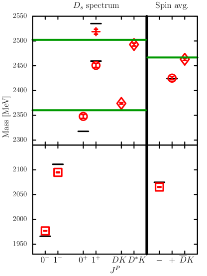
Figure 12: On the left, our final results for the lower lying $D_{s}$ spectrum as detailed in Table 7. The short horizontal black lines indicate the corrected experimental values (see Section II) while the green horizontal lines give the positions of the $DK$ and $D^{*}K$ non-interacting thresholds. Our lattice results for the finite volume thresholds are labelled $DK$ and $D^{*}K$, respectively. The errors indicated are statistical only. On the right, the negative parity spin-averaged $1S$ mass $m_{-}=\frac{1}{4}\left(m_{0^{-}}+3m_{1^{-}}\right)$ is shown and denoted $-$, while the same spin-average of the positive parity $0^{+}$ and $1^{+}$ states is labelled with $+$ and the weighted average of the threshold is labelled as $\overline{D}K$.

Our final results for the lower lying $D_{s}$ spectrum are compiled in Table 7 and displayed in Fig. 12. The energies of the negative parity particles and the thresholds, which display very little dependence on the spatial volume, are taken from the $m_{\pi}=150$ MeV, $L=64a$ ensemble. The masses of the $D_{s0}^{*}(2317)$ and $D_{s1}(2460)$ correspond to the infinite volume values in Table 4 derived from the phase shift analysis of Section V.2. For the $1^{+}$ state above threshold, identified as the $D_{s1}(2536)$, we also found no significant dependence of the mass on the spatial extent, even in the presence of $s$-wave $D^{*}K$ interpolators. This behaviour suggests a small coupling to the threshold (which is difficult to resolve on the lattice via Lüscher’s formalism) and a narrow width. Indeed the experimentally measured width is only approximately $0.8$ MeV for this decay mode Patrignani et al. (2016). It would be interesting to also consider coupling to the $D^{*}K$ in $d$-wave since in the heavy quark limit this mode is dominant for the $j^{P}=\frac{3}{2}^{+}$ doublet of which the $D_{s1}(2536)$ is part, with the $s$-wave channel absent Isgur and Wise (1991) (the opposite holds for the $j^{P}=\frac{1}{2}^{+}$ doublet which contains the $D_{s1}(2460)$). Experimentally, the $s$-wave mode dominates and its contribution to the total width is 0.72(5)(1) Balagura et al. (2008). At present, our best estimate of the physical $D_{s1}(2536)$ energy is again provided by the $m_{\pi}=150$ MeV, $L=64a$ ensemble.

We achieve statistical errors below $0.2\%$ for the positive parity states and even smaller ones for the negative parity states, due to the large number of configurations analysed. Although the overall pattern of energy levels is as expected, at this level of precision, there are clear discrepancies with the experimental spectrum due to the remaining systematics arising from lattice spacing effects and the still unphysical light quark mass. As mentioned in Section II, fine structure splittings are expected to be sensitive to discretisation effects (which begin at $O(a^{2})$ in our study), due to being dominated by high energy scales. We find the hyperfine splittings, $m_{D_{s}^{*}}-m_{D_{s}}=118(1)$ MeV and $m_{1^{+}}-m_{0^{+}}=103(6)$ MeV, are well below the QED and isospin corrected experimental values of $145.3(7)$ and $142(2)$ MeV, respectively. Spin-averaged combinations are less affected, and better agreement is seen as illustrated on the right hand side of Fig. 12 — both the positive parity and threshold averages are reproduced within errors — indicating most of the disagreement observed for the individual masses is likely due to discretisation effects. For the positive parity spin-average we are computing $m_{+}=\frac{1}{4}\left(m_{0^{+}}+3m_{1^{+}}\right)$ for the $\frac{1}{2}^{+}$ doublet, which includes the lower axialvector state. For the threshold we take the spin-average of the $1S$ $D$ mesons masses, $m_{\overline{D}}=\frac{1}{4}(m_{D}+3m_{D^{*}})$, together with the kaon mass.

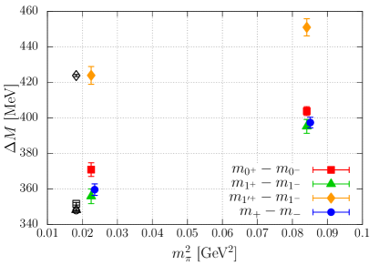
Figure 13: Mass splittings as a function of the pion mass squared for ensembles with a spatial extent of $L=64a$. The corresponding corrected experimental values (see Section II) are indicated as black open symbols at $m_{\pi}=0.135$ GeV. The spin-average of the mass of the lowest lying negative (positive) parity states is denoted $m_{-}$ ($m_{+}$), while $m_{1^{+}}$ ($m_{1^{\prime+}}$) denotes the mass of the lower (higher) $1^{+}$ level. The errors shown are statistical only.

In order to separate the light and strange quark effects from that of the charm quark, we compute the splitting $m_{+}-m_{-}$, displayed in Fig. 13 for the largest spatial extent. The results for $m_{\pi}=290$ MeV are shown for comparison. Heavy quark effects may also largely cancel when considering splittings between masses within the two $j=\frac{1}{2}$ doublets, i.e. $\Delta m_{0}=m_{0^{+}}-m_{0^{-}}$ and $\Delta m_{1}=m_{1^{+}}-m_{1^{-}}$ and possibly between the lower $j_{z}$ components of the $\frac{3}{2}^{+}$ and $\frac{1}{2}^{-}$ doublets, $\Delta m_{1^{\prime}}=m_{1^{\prime+}}-m_{1^{-}}$. The splittings are a few hundred MeV in size as expected for quantities dominated by scales of the order of $\overline{\Lambda}\sim 500$ GeV ($\ll a^{-1}=2.76$ GeV). As mentioned in Section V.2, there is significant dependence on the pion mass which is at odds with a simple charm-strange quark model interpretation of the positive parity states (the masses of the $1S$ negative parity states do not vary significantly with $m_{\pi}$). For $m_{\pi}=150$ MeV, $\Delta m_{1}$ and $\Delta m_{1^{\prime}}$ are reasonably consistent with experiment, while $\Delta m_{0}$ displays a significant difference of around $6\%$. However, for the spin-averaged splitting, for which lattice spacing effects are most effectively suppressed, there is only a 3% discrepancy or 4$\sigma$ in the statistical errors. With a very short (crude) linear extrapolation to the physical point of $m_{\pi}=135$ MeV, we find $356(3)$ MeV for this splitting compared to the physical value of $349(2)$ MeV.

V.5 Decay constants

We are interested in how the magnitude of the ground state $0^{+}$ and $1^{+}$ decay constants compare with those of “conventional” mesons such as the pseudoscalar $D_{s}$ and vector $D^{*}_{s}$. Starting with the $0^{+}$ state, the scalar decay constant, $f_{S}$, is defined through,

$$\braket{0}{\overline{s}c}{D_{s0}^{*}\left(\boldsymbol{p}\right)} = f_{S}m_{0^{+}},$$ (36)

where the physical state is normalised according to

$$\braket{D_{s0}^{*}\left(\boldsymbol{p}\right)}{D_{s0}^{*}\left(\boldsymbol{p}^{\prime}\right)}=2E(\boldsymbol{p})L^{3}\delta_{\boldsymbol{p}\boldsymbol{p}^{\prime}},$$ (37)

for a finite volume $L^{3}$ and $E(\boldsymbol{p})$ is the energy of the state. The conserved vector current relation (CVC) connects $f_{S}$ with the vector decay constant, $f_{V}$,

$$\braket{0}{\overline{s}\gamma_{\mu}c}{D_{s0}^{*}\left(\boldsymbol{p}\right)} = f_{V}p_{\mu},$$ (38)

such that at zero momentum,

$$f_{V}=f_{S}(m_{c}-m_{s})/m_{D_{s0}^{*}},$$ (39)

with $m_{c}$ and $m_{s}$ denoting the charm and strange quark masses, respectively. For a $1^{+}$ state with polarisation $\epsilon_{\mu}$, one can define axialvector and tensor decay constants:

$$\braket{0}{\overline{s}\gamma_{\nu}\gamma_{5}c}{D_{s1}\left(\boldsymbol{p},\boldsymbol{\epsilon}\right)} = f_{A}m_{D_{s1}}\epsilon_{\nu},$$ (40)

$$\braket{0}{\overline{s}\gamma_{5}\sigma_{\mu\nu}c}{D_{s1}\left(\boldsymbol{p},\boldsymbol{\epsilon}\right)} = f_{T}(p_{\mu}\epsilon_{\nu}-p_{\nu}\epsilon_{\mu}),$$ (41)

where since we are at zero spatial momentum, we set $\mu=t$ and average over $\nu=i\in\{1,2,3\}$. The above normalisations are compatible with those for a pseudoscalar meson for which the decay constant $f_{D_{s}}=250(7)$ MeV for $N_{f}=2$, see the FLAG review Aoki et al. (2017) for details. Note that when comparing with the latter, the $0^{+}$ vector and $1^{+}$ axialvector decay constants are the corresponding weak observables, while $f_{S}$ and $f_{T}$ only appear in Standard Model processes beyond tree-level or new physics interactions.

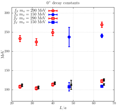
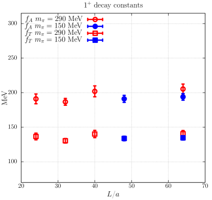
Figure 14: The scalar and vector decay constants of the $D_{s0}^{*}(2317)$ (left) and the axial and tensor decay constants of the $D_{s1}(2460)$ (right) for different pion masses and spatial volumes. The black crosses indicate $f^{\rm CVC}_{V}$, the vector decay constant obtained using $f_{S}$ and the CVC relation, Eq. (39). The errors shown correspond to the statistical and renormalisation uncertainties added in quadrature, see Table 8.

On the lattice, the bare matrix elements are extracted from correlators with a source interpolator, $O^{\dagger}$, which has a good overlap with the physical state, and local sink operators, $J_{S}=\overline{s}c$ and $J_{V}=\overline{s}\gamma_{t}c$ for the $0^{+}$ and $J_{A}=\overline{s}\gamma_{i}\gamma_{5}c$ and $J_{T}=\overline{s}\gamma_{5}\gamma_{t}\gamma_{i}c$ for the $1^{+}$, that are projected onto zero momentum:

$$C^{X}_{LS}(t) = \braket{0}{J_{X}\left(t\right)O^{\dagger}(0)}{0}$$ (42)

$$\approx \sqrt{\frac{mL^{3}}{2}e^{mt_{0}}}f^{\rm latt}_{X}e^{-mt}$$ (43)

with $X\in\{S,V,A,T\}$ and $m\in\{m_{0^{+}},m_{1^{+}}\}$. The source interpolator is constructed from the basis of smeared operators realised for the variational analysis, weighted by the components of the eigenvector of the lowest state. In the limit of ground state dominance, we expect the time dependence shown on the r.h.s., where $t_{0}$ is the reference time in Eq. (4). We perform simultaneous single exponential fits to correlators containing operators with the same quantum numbers, i.e. $C^{S}_{LS}$ and $C^{V}_{LS}$ for the $0^{+}$ and $C^{A}_{LS}$ and $C^{T}_{LS}$ for the $1^{+}$ $D_{s}$ mesons. This ensures the mass in Eq. (43) is consistent for the different decay constants. The resulting masses were also found to be compatible with those extracted from the variational analysis. The correlators relevant for determining the axial and tensor decay constants of the $D_{s1}(2536)$ were also computed in our analysis, however, the simultaneous fits were unsatisfactory and it was not possible to achieve reliable results. For this reason, we do not present values for the decay constants of this resonance.

Table 8: Renormalised decay constants for the $D_{s0}^{*}\left(2317\right)$ and $D_{s1}(2460)$ in MeV for all ensembles. The scalar and tensor decay constants are renormalised in the $\overline{\rm MS}$ scheme at a scale of 2 GeV. The errors given are in the first case statistical and in the second case due to the uncertainty in the renormalisation and improvement factors. For the $m_{\pi}=150$ MeV data the third error is an estimate of finite volume effects while the fourth is the possible order of magnitude of the discretisations effects, see the text.

	$m_{\pi}=290$ MeV				$m_{\pi}=150$ MeV
$L/a$	24	32	40	64	48	64
$D_{s0}^{*}$
$f_{S}^{\rm ren}$ [MeV]	$\>233(8)(2)\>$	$225(8)(2)$	$249(8)(2)$	$270(7)(2)$	$238(25)(2)$	$241(4)(2)(+12)(10)$
$f_{V}^{\rm ren}$ [MeV]	$\>108(3)(2)\>$	$104(4)(2)$	$114(3)(2)$	$123(3)(2)$	$109(11)(2)$	$111(2)(2)(+05)(10)$
$f^{\rm CVC,ren}_{V}$ [MeV]	$\>112(4)(0)\>$	$106(4)(0)$	$117(4)(0)$	$126(3)(0)$	$113(12)(0)$	$114(2)(0)(+05)(10)$
$D_{s1}$
$f_{A}^{\rm ren}$ [MeV]	$\>191(6)(4)\>$	$187(3)(4)$	$202(7)(4)$	$205(6)(4)$	$191(4)(4)$	$194(3)(4)(+5)(10)$
$f_{T}^{\rm ren}$ [MeV]	$\>137(4)(2)\>$	$130(2)(2)$	$140(5)(2)$	$141(4)(2)$	$134(2)(2)$	$135(2)(2)(+3)(10)$

In order to convert the bare results, $f_{X}^{\rm latt}$, into physical predictions the lattice decay constants are renormalised in the $\overline{\rm MS}$ scheme and Symanzik improvement is applied to reduce the discretisation errors to $O(a^{2})$,

$$f_{X}^{\rm ren}=Z_{X}\left(1+a\overline{m}b_{X}\right)f^{\rm latt}_{X},$$ (44)

where $\overline{m}=(m_{c}+m_{s})/2$ and the vector Ward identity quark masses, $m_{q=c,s}=(1/\kappa_{q}-1/\kappa_{\rm crit})/2a$. The critical hopping parameter, $\kappa_{\rm crit}=0.1364281(12)$, was evaluated in Ref. Bali et al. (2015), which also provides non-perturbative values for the renormalisation factors,

$$Z_{A}=0.76487(64),\qquad Z_{V}=0.7365(48),$$

$$Z_{S}=Z^{\overline{\text{M}S}}_{S}(\mu=2\,\text{GeV})=0.6153(25),$$

$$Z_{T}=Z^{\overline{\text{M}S}}_{T}(\mu=2\,\text{GeV})=0.8530(25),$$ (45)

that are updates of earlier determinations in Ref. Göckeler et al. (2010). One loop expressions for the improvement factors $b_{A,V,T}$ were employed Sint and Weisz (1997); Taniguchi and Ukawa (1998); Capitani et al. (2001),

$$b_{A}=1+0.15219(5)g^{2},\qquad b_{V}=1+0.15323(5)g^{2},$$

$$b_{T}=1+0.1392(1)g^{2},$$ (46)

along with the “improved” coupling $g^{2}=-3\ln P=6/\beta+O(g^{4})$. $P$ denotes the plaquette with the normalisation $P=1$ at $\beta=\infty$ and the chirally extrapolated value of $P$ is equal to $0.54988$. The uncertainty due to omitting higher orders of the perturbative expansion is taken to be one half of the one-loop term. For the scalar case, we utilise the non-perturbative determination of $b_{S}$ in Ref. Fritzsch et al. (2010).

The final results are detailed in Fig. 14 and Table 8. In the latter, the first error quoted is statistical, while the second is the uncertainty due to renormalisation and $O(a)$ improvement. The decay constants tend to decrease slightly as the pion mass is reduced and for the $D_{s1}^{*}(2317)$ there is a mild dependence on the spatial lattice extent. We find reasonable consistency with Eq. (39) when we derive the vector $0^{+}$ decay constant from the scalar one, as seen in the figure, suggesting discretisation effects are not severe. We remark that since the combination $f_{S}(m_{c}-m_{s})$ is renormalisation group invariant and is free of additive renormalisation, $f_{V}$ determined in this way (denoted $f_{V}^{\rm CVC}$) does not require knowledge of any renormalisation factors or improvement terms and is automatically $O(a)$ improved. We consider $f_{V}^{\rm CVC}$ to represent the most reliable estimate of the vector decay constant.

Table 9: Comparison of lattice results for the scalar and vector decay constants of $D_{s1}^{*}(2317)$ and the axial decay constant of the $D_{s1}(2460)$ from this work and that of Ref. Herdoiza et al. (2006) with other approaches, in MeV. The errors indicated for our values are, in order, statistical, those arising from the renormalisation and estimates of the uncertainties due to finite volume and lattice spacing. Refs. Hwang and Kim (2005); Cheng and Hou (2003); Cheng and Chua (2006) combine the experimental branching fractions for $B\to D^{(*)}D_{sJ}^{(*)}$ decays with heavy quark symmetry (HQS) and the factorisation approximation, while Refs. Le Yaouanc et al. (2001); Hsieh et al. (2004); Cheng et al. (2004); Verma (2012); Segovia et al. (2012) employ quark models (QM) and Refs. Colangelo et al. (2005); Wang (2015) use QCD sum rules (QCDSR). The study of Ref. Faessler et al. (2007) assumes a $D^{(*)}K$ molecular structure for the $D_{s0}^{*}(2317)$ and $D_{s1}(2460)$ and constrains the parameters of their effective Lagrangian with the experimental $D\rightarrow K^{(*)}$ semileptonic formfactors. See the references for more details.

	$f_{S}^{0^{+}}$ [MeV]	$f_{V}^{0^{+}}$ [MeV]	$f_{A}^{1^{+}}$ [MeV]
This work	241(4)(2)(+12)(10)	114(2)(0)(+5)(10)	194(3)(4)(+5)(10)
LQCD Herdoiza et al. (2006)	340(110)	200(50)
$B$-decays+HQS Hwang and Kim (2005)		74(11)	166(20)
$B$-decays+HQS Cheng and Hou (2003)		67(13)
$B$-decays+HQS Cheng and Chua (2006)		58-86	130-200
QM Le Yaouanc et al. (2001)		440	410
QM Hsieh et al. (2004)		122-154
Light Front QM Cheng et al. (2004)		71	117
Light Cone QCDSR Colangelo et al. (2005)	225(25)		225(25)
$DK$-molecule Faessler et al. (2007)		67.1(4.5)	144.5(11.1)
Light Front QM Verma (2012)		$74.4^{+10.4}_{-10.6}$	$159^{-36}_{+32}$
QM Segovia et al. (2012)		119	165
QCDSR Wang (2015)	333(20)		245(17)

We take the results from the $m_{\pi}=150$ MeV, $L=64a$ ensemble as being closest to the physical values. Unfortunately, the correlators needed to evaluate the negative parity equivalents were not computed, however, a simulation with the same action by the ALPHA collaboration found the pseudoscalar decay constant $f_{D_{s}}\sim 257$ MeV Heitger et al. (2014) at $m_{\pi}=190$ MeV and $a=0.065$ fm with a final continuum, chirally extrapolated value of $247(5)(5)$ MeV. Very little dependence on the pion mass was observed. Considering this result and the FLAG value quoted above, the ($P$-wave) $0^{+}$ vector decay constant is roughly $45\%$ of that of the pseudoscalar, slightly above the estimate of $\sim 0.32$ from non-leptonic $B$ decays to $D^{(*)}D_{sJ}^{(*)}$ but of a similar order of magnitude. The difference is indicative of the size of $1/m_{c}$ corrections and/or violations of the factorisation approximation in the latter approach.

Performing the same comparison for the $D_{s}^{*}$ and $D_{s1}(2460)$ is more difficult as lattice results for the vector meson are only available after continuum and chiral extrapolation for different lattice actions: Becirevic et al. utilising $N_{f}=2$ twisted mass fermions found $f_{Ds^{*}}=311(9)$ MeV and $f_{Ds^{*}}/f_{D_{s}}=1.26(3)$ Becirevic et al. (2012), while for $N_{f}=2+1+1$ HPQCD with the HISQ fermion action obtained $f_{Ds^{*}}/f_{D_{s}}=1.10(2)$ Donald et al. (2014) and the ETM collaboration with twisted mass fermions quoted $f_{Ds^{*}}=268.8(6.6)$ MeV and $f_{Ds^{*}}/f_{D_{s}}=1.087(20)$Lubicz et al. (2017). Taking $f_{Ds^{*}}/f_{D_{s}}$ in the range $1.1-1.3$ and our result for $f_{D_{s1}(2460)}$, gives the latter very roughly as $60-70\%$ of $f_{D_{s}^{*}}$, which is very similar to the estimate from non-leptonic $B$ decays.

With a statistical precision of less than $2\%$ one might expect the systematics arising from finite volume and discretisation effects to be noticeable. We quantify the former by performing a finite volume extrapolation of the $m_{\pi}=290$ MeV data, where we have a sufficient number of spatial volumes, with the leading order chiral form of $f+ge^{-Lm_{\pi}}/(Lm_{\pi})^{3/2}$. The $L=24a$ values are omitted in the fit as higher order terms may be required for $Lm_{\pi}=2.7$. In spite of the proximity of the $D^{(*)}K$ threshold the volume dependence is small and for all decay constants the $L=64a$ data are compatible with the infinite volume limits. From Table 1 the largest volume for $m_{\pi}=150$ MeV is equivalent in terms of $Lm_{\pi}$ to the $L=32a$, $m_{\pi}=290$ MeV ensemble. For fixed $Lm_{\pi}$ and to NLO ChPT finite volume effects are due to one-pion exchange and scale with $g\propto m_{\pi}^{2}$, hence, we estimate these effects to be of the order of

$$\left(f^{290\,\text{MeV}}_{X,L=64a}-f^{290\,\text{MeV}}_{X,L=32a}\right)\times\left(150/290\right)^{2}$$ (47)

in the near physical data. In the case of the $D_{s1}$ at the lighter pion mass one may worry about how to define the decay constants in view of the possibility of a $p$-wave decay to $D_{s}\pi\pi$. The theoretical framework has been developed in Ref. Briceño and Hansen (2015) for two meson channels. An analogous result does not as yet exist for the three body problem, however, in view of the narrowness of the $D_{s1}$ state we would expect such corrections to be very small.

With only one lattice spacing available it is not possible to quantify the magnitude of discretisation effects. Instead, the 10 MeV difference between the $a=0.065$ fm result of the ALPHA collaboration mentioned above and their continuum limit value is taken as an indication of their possible size. This systematic, along with that for finite $L$, is included in Table 8. We remark that the shift in the results from a linear chiral extrapolation in $m_{\pi}^{2}$ to the physical point is below the statistical standard deviation of the $m_{\pi}=150$ MeV results.

Our final results are compared with those of other works in Table 9. To our knowledge there is only one previous lattice study of the decay constants by UKQCD Herdoiza et al. (2006) who employ $N_{f}=2$ non-perturbatively improved clover fermions at a single coarse lattice spacing of $a=0.10$ fm and a small volume with $L=1.6$ fm, without consideration of the coupling to the $DK$ threshold. Their values are above ours but in agreement considering the large uncertainties of their calculation. Our results are also somewhat above those derived from the experimental branching ratios of $B$ decays (under the assumption of heavy quark symmetry and the factorisation approximation), while quark model and QCD sum rule studies give a wide range of values, some of which are consistent with ours.

In the heavy quark limit the $0^{+}$ and $1^{+}$ form a degenerate doublet with $f_{V}^{0^{+}}=f_{A}^{1^{+}}$. At the charm quark mass this equality is violated by 40%, see Table 9. As mentioned above the decay constants are suppressed relative to the corresponding negative parity ones. This suggests the scalar and axialvector particles are more spatially extended as might be expected for $P$-wave states but this is also compatible, for example, with a molecular interpretation. If we look to the charmonium sector as an indication of how conventional $S$- and $P$-wave quark model particles compare, we find the ratio of decay constants for decay to $\gamma\gamma$ between the $J^{PC}=0^{-+}$ $\eta_{c}$ and, the $J^{PC}=0^{++}$ $\chi_{c0}$ is around 0.7.

VI Conclusions

In summary, we have performed a high statistics study of the scalar and axialvector sectors of the $D_{s}$ spectrum involving six volumes comprising linear spatial extents from 1.7 fm up to 4.5 fm and two pion masses of 290 and 150 MeV for a single lattice spacing $a=0.07$ fm. The near physical pion mass enables the $DK$ and $D^{*}K$ thresholds to be realised to within 14 MeV of the QED and isospin corrected experimental values. $S$-wave coupling to the threshold is accounted for in the simulation through the variational approach with a basis of five quark-antiquark interpolators and a single four quark interpolator for each channel. The $D_{s}^{(*)}\eta$ and $D_{s}\pi\pi$ thresholds that also exist in the isospin symmetric limit are not considered.

The four quark operators were found to be essential for reliably extracting the ground state and first scattering levels in our setup while in the axialvector channel the third state, identified as the $D_{s1}(2536)$, could be resolved sufficiently using quark-antiquark interpolators only. The gap between the first and second scattering levels is not large for the biggest volumes and the analysis could be improved in the future with the inclusion of operators representing the $D$ and $K$ mesons with opposite momenta. The quark line diagrams were evaluated following the stochastic approach of Refs. Aoki et al. (2007, 2011); Bali et al. (2016). The limited basis of interpolators required means this approach is substantially cheaper in terms of the computer time compared to other methods such as the distillation technique Peardon et al. (2009); Morningstar et al. (2011) and enables large volumes and small pion masses to be realised.

The energy spectrum is translated into values for the phase shift above and below the threshold via Lüscher’s formalism. The data were consistent with a linear dependence on the energy squared, within the range $|p^{2}|\leq 300$ GeV², as expected in the effective range approximation. The results for the smallest spatial extent of $L=24a\approx 1.7$ fm lie outside this region and may suffer from exponentially suppressed finite volume effects which are not included in the Lüscher approach or may be in the range where corrections to linear behaviour are significant. Our values for the scattering length, effective range, binding energy and coupling to the threshold are given in Table 4. The scattering lengths are negative, compatible with the existence of a bound state in each channel and the infinite volume masses are consistent with the results from the largest spatial extent of 4.5 fm. The phase shift was not evaluated for the $D_{s1}(2536)$ state due to the lack of sensitivity of the mass to the spatial volume.

A complementary analysis within the chiral unitary approach provided very similar results for the bound state masses and couplings, see Table 5. One can also access Weinberg’s compositeness probability $1-Z$, which we found to be 1 within errors for both states. A large value for the latter is often interpreted as indicating the bound state has a substantial $DK$ component in the wavefunction.

The final results for the spectrum are compiled in Table 7 and displayed in Fig. 12. They are comprised of masses of the $0^{+}$ and lower $1^{+}$ state derived from the phase shift analysis of the $m_{\pi}=150$ MeV ensemble and the energies of the negative parity levels and higher $1^{+}$ state obtained on the largest spatial volume at this pion mass. Due to the high statistical precision achieved, significant disagreement is seen with experiment, in particular for fine structure splittings. The splitting of the $0^{+}$ state with the $DK$ threshold is also well below the physical result, while that for the $1^{+}$ level is consistent. These differences with respect to experiment seem to be predominantly due to lattice spacing effects, as reasonable agreement is observed for spin-averaged quantities, for example, for the average threshold splitting and average $j^{P}=\frac{1}{2}^{+}$, $\frac{1}{2}^{-}$ splitting. Further simulations at finer lattices are required to remove this source of systematics.

The masses of the scalar and both axialvector particles are sensitive to the pion mass, suggesting that these may not be conventional quark model states. A heavier light quark mass leads to more strongly bound $D_{s0}^{*}$ and $D_{s1}$ mesons. Evaluation of the decay constants of these mesons provides additional inputs to model calculations probing their internal structure. We find $f_{V}^{0^{+}}=114(2)(0)(+5)(10)$ MeV and $f_{A}^{1^{+}}=194(3)(4)(+5)(10)$ MeV, where the errors are due to statistics, renormalisation, finite volume and lattice spacing effects. The ratios with the negative parity equivalents are of similar sizes to those extracted from analyses of non-leptonic $B$ decays to $D^{(*)}D_{sJ}^{(*)}$ Datta and O’Donnell (2003); Hwang and Kim (2005); Cheng and Chua (2006), exploiting the factorisation approximation within HQET. However, our $f_{V}^{0^{+}}$ comes out somewhat higher hinting at violations of the approximations. Finally we also computed the scalar and tensor decay constants of the $0^{+}$ and $1^{+}$ mesons, respectively, $f_{S}^{0^{+}}=241(4)(2)(+12)(10)$ MeV and $f_{T}^{1^{+}}=135(2)(2)(+3)(10)$ MeV. These are not accessible via leading order Standard Model processes but it would be interesting to see if any model calculation can reproduce these numbers.