Asteroid shapes and thermal properties from combined optical and mid-infrared photometry inversion

Abstract

Context. Optical lightcurves can be used for the shape and spin reconstruction of asteroids. Due to unknown albedo, these models are scale-free. When thermal infrared data are available, they can be used for scaling the shape models and for deriving thermophysical properties of the surface by applying a thermophysical model.

Aims. We introduce a new method of simultaneous inversion of optical and thermal infrared data that allows the size of an asteroid to be derived along with its shape and spin state.

Methods. The method optimizes all relevant parameters (shape and its size, spin state, light-scattering properties, thermal inertia, surface roughness) by gradient-based optimization. The thermal emission is computed by solving the 1-D heat diffusion equation. Calibrated optical photometry and thermal fluxes at different wavelengths are needed as input data.

Results. We demonstrate the reliability and test the accuracy of the method on selected targets with different amount and quality of data. Our results in general agree with those obtained by independent methods.

Conclusions. Combining optical and thermal data into one inversion method opens a new possibility for processing photometry from large optical sky surveys with the data from WISE. It also provides more realistic estimates of errors of thermophysical parameters.

1 Introduction

Optical and thermal infrared disk-integrated radiation of asteroids is routinely used for the determination of their physical properties (Kaasalainen et al., 2002; Harris & Lagerros, 2002; Ďurech et al., 2015; Delbo et al., 2015, and references therein). The reflected sunlight at optical wavelengths serves as the first guess for the size of the asteroids (from the brightness) and taxonomic type (color information). The periodic variations of the brightness due to rotation carry information about the shape and spin state of the asteroid. A mathematically robust and reliable method of reconstruction of asteroid’s shape and spin state from disk-integrated reflected light was developed by Kaasalainen & Torppa (2001) and Kaasalainen et al. (2001). The method has been successfully applied to hundreds of asteroids (Ďurech et al., 2009; Hanuš et al., 2011, 2016; Marciniak et al., 2011; Ďurech et al., 2016, for example) and its results were confirmed by independent methods (Kaasalainen et al., 2005; Marchis et al., 2006; Keller et al., 2010; Ďurech et al., 2011). Due to the ill-posedness of the general inverse problem in case of disk-integrated data, the shape is usually modelled as convex, because this approach guarantees uniqueness of the model. The output of the lightcurve inversion method is a shape model represented by a convex polyhedron that approximates the real nonconvex shape of an asteroid. Because of the ambiguity between size $D$ and geometric albedo $p_{\text{V}}$, the models are scale free. The visible flux is proportional to $D^{2}p_{\text{V}}$ and in principle $0.01\lesssim p_{\text{V}}\lesssim 1.0$ (Masiero et al., 2011), so size estimation from the visible brightness has a very large uncertainty. The models can be set to scale by disk-resolved data (Hanuš et al., 2013a), stellar occultation silhouettes (Ďurech et al., 2011), or thermal infrared data (Hanuš et al., 2015).

The transition from purely reflected light to purely thermal emission is continuous and the transition zone where the detected flux is a mixture of reflected solar radiation and thermal emission depends on the heliocentric distance, albedo, and thermal properties of the surface. For asteroids in the main-belt it is around 3–5 $\mu$m (Delbó & Harris, 2002; Harris & Lagerros, 2002). For longer wavelengths, the flux can be treated as pure thermal emission. Measurements of this flux can be used for direct estimation of the size and sophisticated thermal models have been developed to reveal thermal properties of the surface from measurements of thermal emission at different wavelengths.

The simplest approach to thermal modelling that is often used when no information about the shape is available is to assume that the shape is a sphere. Then the standard thermal model (STM, Lebofsky et al., 1986) or the near-Earth asteroid thermal model (NEATM, Harris, 1998) are used. When interpreting thermal data by a thermophysical model (TPM), the shape and spin state of the asteroid has to be known to be able to compute the viewing and illumination geometry for each facet on the surface (and shadowing in case of a nonconvex model). Usually, the 1-D heat diffusion problem is solved in the subsurface layers. There are many different TPM codes, they differ mainly in the way they deal with surface roughness (for a review, see Delbo et al., 2015). Shape models are usually reconstructed from other data sources like photometry (Kaasalainen et al., 2002), radar echos (Benner et al., 2015), or high-angular-resolution imaging (Carry et al., 2010a). Although this approach in general works and provides thermophysical parameters, the main caveat here is that the shape and spin state are taken as a priori and their uncertainties are not taken into account. This may lead to underestimation of errors of the derived parameters or even erroneous results (see Rozitis & Green, 2014; Hanuš et al., 2015, for example).

To overcome the limitation of a two-step approach where first the shape/spin model is created and then thermal data are fitted, we have developed a new algorithm that allows for simultaneous optimization of all relevant parameters. We call it convex inversion TPM (CITPM) and we describe the algorithm in Sect. 2 and show how this method works for some test asteroids in Sect. 3.

2 Combined inversion of optical and thermal infrared data

Our new code joins two widely used and well tested methods: (i) the lightcurve inversion of Kaasalainen et al. (2001) and (ii) the thermophysical model of Lagerros (1996, 1997, 1998). We use the convex approach, which enables us to work in the Gaussian image representation: The convex shape is represented by areas of surface facets and corresponding normals. The normals are fixed while the areas are optimized to get the best agreement between the visible light and the thermal infrared fluxes calculated by the model and the observed fluxes. Moreover, the distribution of individual areas is parametrized by spherical harmonics (usually of order and degree of six to eight). The polyhedral representation of the shape is then reconstructed by the Minkowski iteration (Kaasalainen & Torppa, 2001). The spin vector is parametrized by the direction of the spin axis in ecliptic coordinates $(\lambda,\beta)$ and the sidereal rotation period $P$. Together with the initial orientation $\varphi_{0}$ at epoch JD₀, these parameters uniquely define the orientation of the asteroid in the ecliptic coordinate frame (Ďurech et al., 2010). With known positions of the Sun and Earth with respect to the asteroid, the illumination and viewing geometry can be computed for each facet. As we work with convex shapes only, there is no global shadowing by large-scale topography in our model, although the generalization of the problem with nonconvex shapes is straightforward, similarly as in the case of lightcurve inversion.

For computing the brightness of an asteroid in visible light, we use Hapke’s model with shadowing (Hapke, 1981, 1984, 1986). This model has five parameters: the average particle single-scattering albedo $\varpi_{0}$, the asymmetry factor $g$, the width $h$ and amplitude $B_{0}$ of the opposition effect, and the mean surface slope $\bar{\theta}$ . We compute Hapke’s bidirectional reflectance $r(i,e,\alpha)$ for each surface element, where $i$ is the incidence angle, $e$ is the emission angle, and $\alpha$ is the phase angle. The total flux scattered towards an observer is computed as a sum of contributions from all visible and illuminated facets.

In standard TPM methods, the size of the asteroid $D$ in kilometers and its geometric albedo $p_{\text{V}}$ are connected via Bond albedo $A_{\text{B}}$, phase integral $q$, and absolute magnitude $H_{0}$ with formulas (see Harris & Lagerros, 2002, for example):

$$D=\frac{1329}{\sqrt{p_{\text{V}}}}\,10^{-\frac{H_{0}}{5}},\qquad A_{\text{B}}=qp_{\text{V}}\,.$$ (1)

However, Bond albedo $A_{\text{B}}$ as well as geometric visible albedo $p_{\text{V}}$ are not material properties and they are unambiguously defined only for a sphere. So instead of this traditional approach, we use a self-consistent model, where the set of Hapke’s parameters is also used to compute the total amount of light scattered to the upper hemisphere, which defines the hemispherical albedo $A_{\text{h}}$ (the ratio of power scattered into the upper hemisphere by a unit area of the surface to the collimated power incident on the unit surface area, Hapke, 2012) needed for computing the energy balance between incoming, emitted, and reflected flux. This hemispherical albedo is dependent on the angle of incidence (it is different for each surface element) and it is at each step computed by numerically evaluating the integral

$$A_{\text{h}}(i)=\frac{1}{\mu_{0}}\int_{\Omega}r(i,e,\alpha)\,\mu\,\mathrm{d}\Omega\,,$$ (2)

where $\mu=\cos e$, $\mu_{0}=\cos i$, and the integration region $\Omega$ is over the upper hemisphere. Because the above defined quantities are in general dependent on the wavelength $\lambda$, we need bolometric hemispherical albedo $A_{\text{bol}}$ that is the average of the wavelength-dependent hemispherical albedo $A_{\text{h}}(\lambda)$ weighted by the spectral irradiance of the Sun $J_{\text{S}}(\lambda)$:

$$A_{\text{bol}}=\frac{\int_{0}^{\infty}A_{\text{h}}(\lambda)J_{\text{s}}(\lambda)\,\mathrm{d}\lambda}{\int_{0}^{\infty}J_{\text{s}}(\lambda)\,\mathrm{d}\lambda}\,.$$ (3)

In practice, we approximate the integrals by sums. The dependence of $A_{\text{h}}$ on $\lambda$ is not know neither from theory nor measurements, so we assume that it is the same as the dependence of the physical (geometric) albedo $p(\lambda)$ that can be estimated from reflectance curves. If asteroid’s taxonomy is known, we take the spectrum of that class in the Bus-DeMeo taxonomy (DeMeo et al., 2009), and extrapolate the unknown part outside the 0.45–2.45 $\mu$m interval with flat reflectance. We then multiply this spectrum by the spectrum of the Sun, taken from Gueymard (2004). If the taxonomic class is unknown, we assume flat reflectance, i.e., $A_{\text{h}}(\lambda)=\text{constant}$.

Both Bond and geometric albedos can be computed from Hapke’s parameters but they are not used in our model directly. We also do not need the formalism of HG system (Bowell et al., 1989). Similarly as geometric albedo, the $H_{0}$ value is properly defined only for a sphere, for a real irregular asteroid it depends on the aspect angle. So instead of using $H_{0}$ and $p_{\text{V}}$, we use directly the calibrated magnitudes on the phase curve. With disk-integrated photometry and a limited coverage of phase angles, it is usually not possible to uniquely determine the Hapke’s parameters. In such cases, they (or a subset of them) can be fixed at some typical values (see Table 6 of Li et al., 2015).

Parameters of the thermophysical model are the thermal inertia $\Gamma$, the fraction of surface covered by craters $\rho_{\text{c}}$ and their opening angle $\gamma_{\text{c}}$ (Lagerros, 1998). The roughness parameter $\bar{\theta}$ of Hapke’s model can be set to the value corresponding to craters or set to a different value, which would mean that there are two values of roughness in the model, one for optical and one for infrared wavelengths. Usually, we use just one value, which makes the model simpler and also more self-consistent.

To find the best-fitting parameters, we use the Levenberg-Marquardt algorithm. The parameters are optimized to give the lowest value for the total $\chi^{2}$ that is composed from the visual and infrared part weighted by $w$:

$$\chi^{2}_{\text{total}}=\chi^{2}_{\text{VIS}}+w\chi^{2}_{\text{IR}}\,.$$ (4)

The visual part is computed as a sum of squares of differences between the observed flux $F_{\text{VIS, obs}}$ and the modelled flux $F_{\text{VIS, model}}$ over individual data points $i$ weighted by the measurement errors $\sigma_{i}$:

$$\chi^{2}_{\text{VIS}}=\sum_{i}\left(\frac{F_{\text{VIS, obs}}^{(i)}-F_{\text{VIS, model}}^{(i)}}{\sigma_{i}}\right)^{2}\,.$$ (5)

The model flux is computed as a sum over all illuminated and visible surface elements $k$:

$$F_{\text{VIS, model}}=\frac{F_{\text{in}}}{\Delta^{2}}\sum_{k}r_{k}\,\mu_{k}\,\delta\sigma_{k}\,,$$ (6)

where $F_{\text{in}}$ is the incident solar irradiance, $\Delta$ is the distance between the observer and the asteroid, $r$ is Hapke’s bidirectional reflectance, $\mu$ is cosine of the emission angle, and $\delta\sigma$ is area of the surface element. If the photometry is not calibrated and we have only relative lightcurves, the corresponding $\chi^{2}$ part is computed such that only the relative fluxes are compared:

$$\chi^{2}_{\text{rel}}=\sum_{j}\sum_{i}\left(\frac{F_{\text{VIS, obs}}^{(j)(i)}}{\bar{F}_{\text{VIS, obs}}^{(j)}}-\frac{F_{\text{VIS, model}}^{(j)(i)}}{\bar{F}_{\text{VIS, model}}^{(j)}}\right)^{2}\,,$$ (7)

where $j$ is an index for lightcurves, $i$ is an index for individual points of a lightcurve, and $\bar{F}^{(j)}$ is the mean brightness of the $j-$th lightcurve.

Similarly, for the IR part of the $\chi^{2}$ we compute

$$\chi^{2}_{\text{IR}}=\sum_{i}\left(\frac{F_{\text{IR, obs}}^{(i)}-F_{\text{IR, model}}^{(i)}}{\sigma_{i}}\right)^{2}\,,$$ (8)

where we compare the observed thermal flux $F_{\text{IR, obs}}$ with the modelled flux $F_{\text{IR, model}}$ at some wavelength $\lambda$. The disk-integrated flux is a sum of contributions from all surface elements that are visible to the observer:

$$F_{\text{IR, model}}=\frac{\epsilon}{\Delta^{2}}\sum_{k}B(\lambda,T_{k},\rho_{\text{c}},\gamma_{\text{c}})\,\mu_{k}\,\delta\sigma_{k}\,,$$ (9)

where $\epsilon$ is the emissivity (assumed to be independent on $\lambda$), and $B$ is radiance of a surface element at temperature $T$ that depends on the wavelength $\lambda$ (blackbody radiation) and includes also a model for macroscopic roughness parametrized by $\rho_{\text{c}}$ and $\gamma_{\text{c}}$. To compute $B$, we have to solve the heat diffusion equation for each surface element and compute $T_{k}$. Assuming that the material properties do not depend on temperature, we solve

$$\rho C\frac{\partial T}{\partial t}=\kappa\frac{\partial^{2}T}{\partial z^{2}}\,,$$ (10)

where the density $\rho$, heat capacity $C$, and thermal conductivity $\kappa$ are combined into a single parameter thermal inertia $\Gamma=\sqrt{\rho C\kappa}$ (Spencer et al., 1989; Lagerros, 1996). Instead of the real subsurface depth $z$, the problem is then solved in the units of the thermal skin depth, which is related to the rotation period and the thermal properties of the material. The boundary condition at the surface ($z=0$) is the equation for energy balance:

$$(1-A_{\text{bol}})\frac{F_{\sun}}{r^{2}}\mu_{0}=\epsilon\sigma T^{4}-\kappa\frac{\partial T}{\partial z}\,,$$ (11)

where the left side of the equation is the energy absorbed by the surface ($F_{\sun}$ is solar irradiance at 1 au, $r$ is the distance from the Sun, and $\mu_{0}$ is cosine of the incidence angle) and the right side is the radiated flux ($\sigma$ is the Stefan-Boltzmann constant) minus the heat transported inside the body. The inner boundary condition is

$$\left.\frac{\partial T}{\partial z}\right|_{z\rightarrow\infty}=0\,,$$ (12)

where $z\rightarrow\infty$ in practice means few skin depths. Eq. (10) is solved by the simplest explicit method with typically tens of subsurface layers.

The weight $w$ in eq. (4) is set such that there is a balance between the level of fit to lightcurves and thermal data. Objectively, the optimum value can be found with the method proposed by Kaasalainen (2011) with the so-called maximum compatibility estimate, which corresponds to the maximum likelihood or maximum a posteriori estimates in the case of a single data mode.

Because of strong correlation between the thermal inertia $\Gamma$ and the surface roughness, the parameters describing the surface fraction covered by craters $\rho_{\text{c}}$ and their opening angle $\gamma_{\text{c}}$ and likewise the parameter $\bar{\theta}$ in Hapke’s model are the only three parameters that are not optimized. They are held fixed and their best values are found by running the optimization many times with different combination of these parameters. The dependence of $\chi^{2}_{\text{total}}$ on $\Gamma$ shows usually only one minimum (sharp or shallow depending on the amount and quality of thermal data), which makes convergence in $\Gamma$ robust and the gradient-based optimization converges to the best value of $\Gamma$ even if started far from it. The emissivity $\epsilon$ is held fixed. Its value can be set to anything between 0 and 1, but in all tests in the following section we used the “standard” value $\epsilon=0.9$. This is a typical value of the emissivity of meteorites and of the minerals included in meteorites obtained in the lab at wavelengths around 10 $\mu$m. This value can significantly change at longer wavelengths, see Delbo et al. (2015) for discussion.

3 Testing the method on selected targets

We tested our method on selected targets, each representing a typical amount of data. First, we used asteroid (21) Lutetia for which there are plenty of photometry and thermal infrared data available and the shape is known from Rosetta spacecraft fly-by. So it is an ideal target for comparing the results from our inversion with ground truth from Rosetta. Another test asteroid with known shape is (2867) Šteins, but in this case thermal data are scarce, so this example should show us the limits of the method. Then we have selected asteroid (306) Unitas – a typical example of an asteroid with enough lightcurves and some thermal data from IRAS and WISE satellites. As the last example, we show on asteroid (220) Stephania how thermal data in combination with sparse optical photometry can lead to a unique model – this is perhaps the most important aspect of the new method that can lead to production of new asteroid models in the future.

3.1 Data

The success of the method is based on the assumption that we have accurately calibrated absolute photometry of an asteroid covering a wide interval of phase angles – to be able to use Hapke’s photometric model and derive the hemispherical albedo. Because most of the available lightcurves are only relative, we used also the Lowell Observatory photometric database (Oszkiewicz et al., 2011; Bowell et al., 2014) as the source of absolutely calibrated photometry in V filter. The only asteroid for which we had enough reliable absolutely calibrated dense lightcurves was (21) Lutetia. As regards thermal data, we used IRAS catalogue (Tedesco et al., 2004), WISE data (Wright et al., 2010; Mainzer et al., 2011), and also Spitzer and Herschel observations for (21) Lutetia. The number of dense lightcurves (usually relative), sparse data points (calibrated), and IR data points for all targets is listed in Table 1. The comparison between CITPM models and independent models is shown in Table 2 in terms of derived physical parameters.

3.2 (21) Lutetia

Because for this asteroid there are lot of lightcurves that well define the convex shape, we do not expect any significant improvement of the model with respect to the two-step method. However, Lutetia with its abundant photometric and infrared data set is a good test case for the new algorithm.

A convex model of Lutetia was derived by Torppa et al. (2003) and later Carry et al. (2010b) created a nonconvex model that was confirmed by the Rosetta fly-by (Carry et al., 2012). The detailed shape model of Lutetia reconstructed from the fly-by imaging (Sierks et al., 2011) can serve as a ground-truth comparison with our model (although part of the surface was not seen by Rosetta and was reconstructed from lightcurves). There are also abundant optical and thermal infrared data for this asteroid – 59 lightcurves observed between 1962 and 2010, out of which 20 are calibrated in V filter, and thermal infrared data (O’Rourke et al., 2012) from 7.87 (Spitzer) to 160 $\mu$m (Herschel PACS). We have not included the Herschel SPIRE data observed at 250, 350, and 500 $\mu$m, because at these long wavelengths the emissivity assumption of $\epsilon=0.9$ is no longer valid (see the discussion in Delbo et al., 2015, for example).

The comparison between our model reconstructed from disk-integrated lightcurves and thermal data and that reconstructed by Sierks et al. (2011) from Rosetta fly-by images is shown in Fig. 1. The volume-equivalent diameter of Rosetta-based model is $98\pm 2$ km, while our model has diameter of $101\pm 4$ km. Our thermal inertia of 30–50  J m^-2 s^-0.5 K^-1 is significantly higher than the value $\sim 5$  J m^-2 s^-0.5 K^-1 of O’Rourke et al. (2012), at the boundary of interval $<30$  J m^-2 s^-0.5 K^-1 given by Keihm et al. (2012), and consistent with the value of $\leq 100$  J m^-2 s^-0.5 K^-1 of Mueller et al. (2006) derived from IRAS and IRTF (InfraRed Telescope Facility) data. The discrepancy between our value and those by O’Rourke et al. (2012) and Keihm et al. (2012) might be partly caused by the fact that we used only wavelengths $\leq 160\,\mu$m, while the lower values of thermal inertia were derived from data sets containing also sub-millimeter and millimeter wavelengths. Longer wavelengths “see” deeper in the subsurface, which is colder than the surface layers. Since $\Gamma$ depends on the temperature, we expect to see $\Gamma$ decreasing with depth, provided the density and packing of the regolith is independent on the depth, which might not be the case. For example, on the Moon the regolith density increases with depth (Vasavada et al., 2012). Harris & Drube (2016) claim to see the same effect on asteroids.

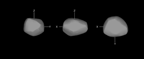
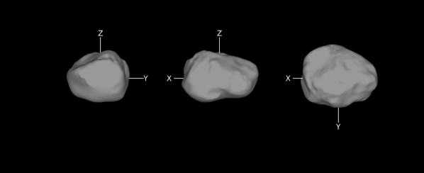
Figure 1: Comparison between the shape of (21) Lutetia reconstructed by our method (top) and that reconstructed by Sierks et al. (2011) from Rosetta fly-by images (bottom).

3.3 (306) Unitas

Unitas is a typical example of a main belt asteroid for which there are some data from both IRAS and WISE (see Tab. 1). The first convex model was published by Ďurech et al. (2007) with pole ambiguity that was later resolved with IR data by Delbo & Tanga (2009) and confirmed with a fit to stellar occultation data by Ďurech et al. (2011). The new CITPM shape model obtained from combined inversion of optical lightcurves and thermal data has the pole direction $(\lambda,\beta)=(82^{\circ},-30^{\circ})$ and the shape similar (Fig. 2) to the old model with pole direction of $(79^{\circ},-35^{\circ})$. The size of the formally best-fitting model (derived independently on the occultation) is $48.7\pm 0.7$ km, which is very close to the size $49\pm 5$ km obtained by scaling the lightcurve-based model to occultation chords. For comparison, the size from the IRAS observation is $46.7\pm 2.3$ km (Tedesco et al., 2004), from WISE $51.6\pm 6.3$ km (Masiero et al., 2011), and from AKARI $46.2\pm 0.6$ km (Usui et al., 2011).

The comparison between the model silhouette and the fit to occultation is shown in Fig. 3, where the red contour corresponds to our new model (no scaling, rms residual 1.7 km) and the blue one corresponds the the model of Ďurech et al. (2007) (rms residual 1.9 km) that was scaled to provide the best fit to the chords. The fit between the model and observations is formally very good (Fig. 4) with reduced $\chi^{2}_{\text{IR}}$ as low as $\sim 0.7$ for thermal inertia in the range 10–100 J m^-2 s^-0.5 K^-1. Delbo & Tanga (2009) applied TPM on only IRAS data and derived systematically higher thermal inertia 100–260 J m^-2 s^-0.5 K^-1 and also size 55–56 km – this demonstrates the fact that with a fixed shape and spin as an input for TPM, the uncertainties of thermophysical parameters are often underestimated (see also Hanuš et al., 2015).

As can be seen in Fig. 2, adding IR data changed the shape model only slightly, but they allowed correct scaling of the size that can be independently checked by occultation in Fig. 3.

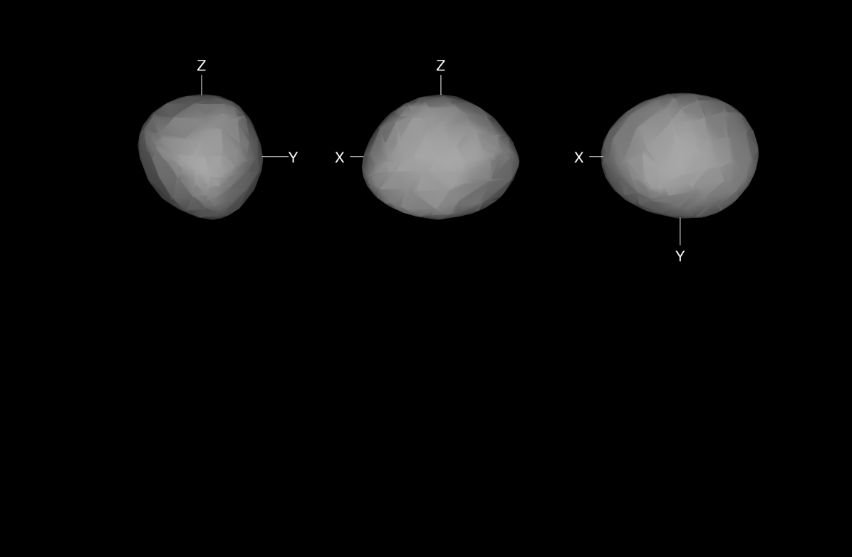
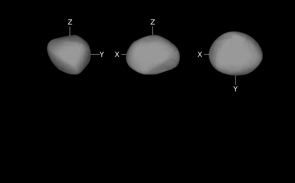
Figure 2: Comparison between the new shape of (306) Unitas reconstructed from thermal and optical data (top) and that reconstructed only from dense optical lightcurves by Ďurech et al. (2007) (bottom).

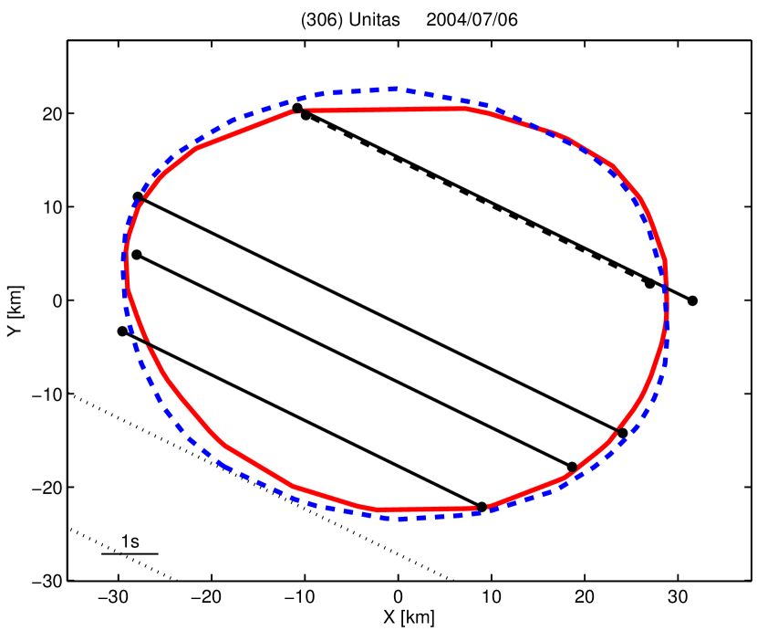
Figure 3: The plane-of-the-sky silhouettes of (306) Unitas for the time of the occultation. The red solid silhouette corresponds to our model, the blue dashed one corresponds to the model from Ďurech et al. (2007). The black lines represent chords reconstructed from timings and positions of individual observers. The dashed chord represents a visual observation with uncertain timing, the dotted lines are a negative observations with no occultation detected. Occultation data were taken form Dunham et al. (2016)

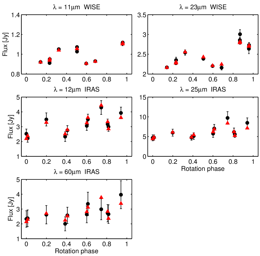
Figure 4: Measured IR fluxes (black circles) of (306) Unitas and the model fluxes for our model (red triangles).

3.4 (2867) Šteins

Similarly to Lutetia, also for this asteroid we have a detailed shape model reconstructed from the Rosetta fly-by images and lightcurves (Jorda et al., 2012). But contrary to Lutetia, thermal data for Šteins are limited to only twelve pairs of WISE data with relative accuracy of 7% and 15% in W3 and W4 filter, respectively. Therefore the thermal properties are poorly constrained. Models with the diameter in the range 5.6–6.2 km and the thermal inertia 70–370 J m^-2 s^-0.5 K^-1 provide an acceptable fit to both thermal and optical data. There is a correlation between these two parameters – solutions with smaller diameter have also lower thermal inertia. The geometric visible albedo is in the range 0.4–0.5. One of the possible shape models is shown in Fig. 5 and the fit to the thermal data in Fig. 6. The selected model has an equivalent diameter of 5.8 km and thermal inertia of 200 J m^-2 s^-0.5 K^-1. For comparison, the shape reconstructed from Rosetta images and lightcurves has the equivalent diameter $5.26\pm 0.26$ km (Jorda et al., 2012). The main difference between the CITPM model and that of (Jorda et al., 2012) is that the Rosetta-based model is much more flat than CITPM model, which might be also the reason why our model has larger equivalent diameter. Leyrat et al. (2011) derived from VIRTIS/Rosetta measurements the thermal inertia $\Gamma=110\pm 13$ J m^-2 s^-0.5 K^-1 for a smooth surface and $\Gamma=210\pm 30$ J m^-2 s^-0.5 K^-1 when a small-scale roughness was included. Spjuth et al. (2012) determined the geometric albedo $0.39\pm 0.02$ at 670 nm from disk-resolved photometry. This shows that with low-quality thermal data, the combined inversion is still possible, but the derived physical parameters have large uncertainties.

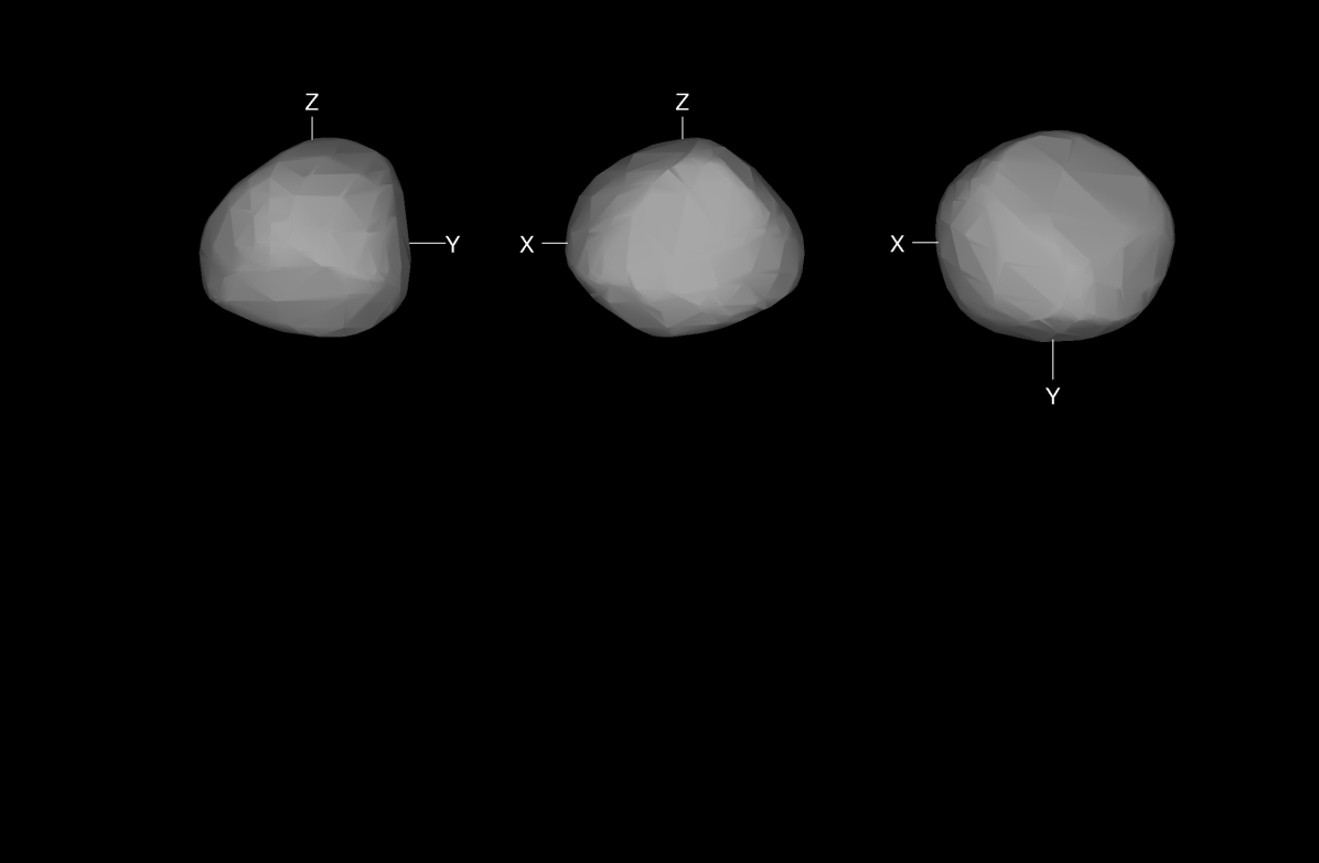
Figure 5: Comparison between the shape of (2867) Šteins reconstructed by our method (top) and that reconstructed by Jorda et al. (2012) from Rosetta fly-by images and lightcurves (bottom).

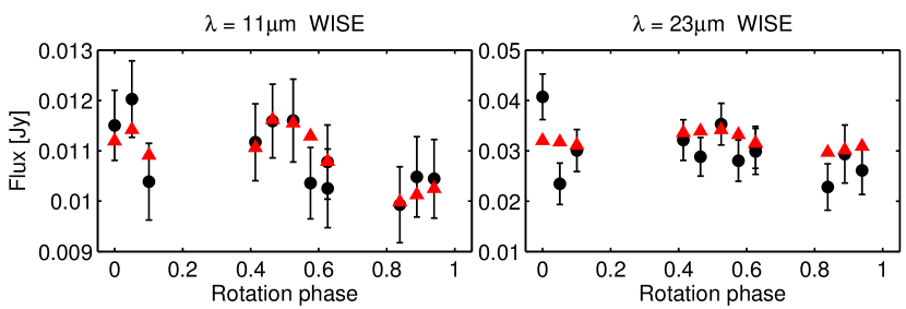
Figure 6: Measured IR fluxes (black circles) of (2867) Šteins and the model fluxes for our model (red triangles).

3.5 (220) Stephania

As the last example we selected an asteroid for which optical data are not sufficient to derive a unique model. To demonstrate the potential of combining sparse photometry with WISE data, we selected asteroid (220) Stephania that was modelled by Hanuš et al. (2013b) from a set of nine lightcurves and sparse data from the US Naval Observatory and the Catalina Sky Survey. The pole direction was $(26^{\circ},-50^{\circ})$ or $(223,-62^{\circ})$. Here we use only Lowell sparse photometry and WISE data in W1 (8 points) and W2 (7 points) for the period determination by the lightcurve inversion method of Kaasalainen et al. (2001). As is shown in Fig. 7, sparse data alone are not sufficient to determine the rotation period uniquely. In the periodogram, there are many possible periods (and corresponding models) that provide the same level of fit for the data. However, adding WISE data from W1 and W2 filters and assuming that they can be treated as reflected light (Ďurech et al., 2016), the correct period of about 18.2 h gives now the global minimum in the periodogram. Even if the number of WISE data points is small compared to the Lowell data ($\sim 400$ points), they were observed within an interval of one day and their contribution to constraining the period is significant. Then, this period is used as a start point for the CITPM model combining now only Lowell photometry, WISE thermal data in W3 and W4 filters, and IRAS data. The best model has pole directions $(24^{\circ},-60^{\circ})$ or $(224^{\circ},-59^{\circ})$ and thermophysical parameters $\Gamma=15^{+60}_{-10}\,$ J m^-2 s^-0.5 K^-1, $D=32.2^{+2.0}_{-0.2}$ km, $p_{\text{V}}=0.075\pm 0.15$. The fit to the IRAS and WISE thermal data is shown in Fig. 8. The rotation phase shift between the optical and thermal lightcurves is very small, only about $10^{\circ}$, which justifies the use of thermal data for period determination.

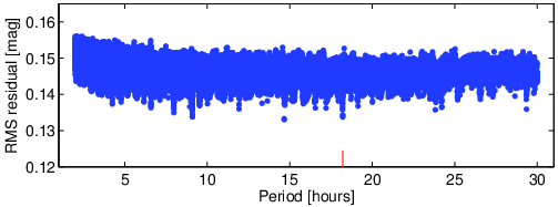
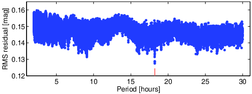
Figure 7: Period search for (220) Stephania for Lowell photometry (top) and Lowell + WISE W1 and W2 data (bottom). The correct rotation period of 18.2 h is marked with a red tick.

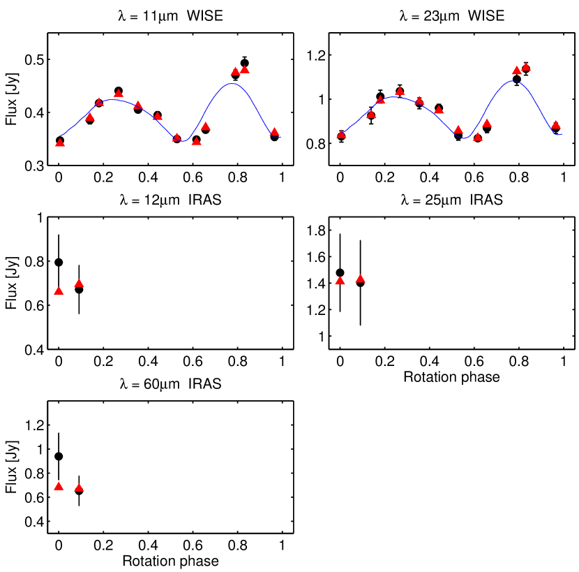
Figure 8: Measured IR fluxes (black circles) of (220) Stephania and the model fluxes for our model (red triangles). The WISE data are shown together with the synthetic optical lightcurve (blue) produced by the model.

Table 1: Number of dense lightcurves $N_{\text{lc}}$, sparse data points $N_{\text{sp}}$, and IRAS and WISE observations. The goodness of fit to thermal data is expressed by the reduced $\chi^{2}_{\text{IR}}$

Asteroid		$N_{\text{lc}}$	$N_{\text{sp}}$	IRAS				WISE		reduced $\chi^{2}_{\text{IR}}$
				$12\,\mu$m	$25\,\mu$m	$60\,\mu$m	$100\,\mu$m	$11\,\mu$m	$22\,\mu$m
21	Lutetia	59		5	5	5	9			0.80
220	Stephania		397	2	2	2		11	11	0.58
306	Unitas	15	386	11	11	11		10	13	0.68
2867	Šteins	21	614					12	12	0.77

Table 2: Comparison between our CITPM models and independent results. The physical parameters are the ecliptic longitude $\lambda$ and latitude $\beta$ of the spin axis direction, the volume-equivalent diameter $D$, the geometric albedo $p_{\text{V}}$, and the thermal inertia of the surface $\Gamma$.

Asteroid		$\lambda$	$\beta$	$D$	$p_{\text{V}}$	$\Gamma$	References
		[deg]	[deg]	[km]		J m-2 s-0.5 K-1
21	Lutetia	56	$-7$	$101\pm 4$	0.19–0.23	30–60	CITPM ($3\sigma$ errors)
		$52.2\pm 0.4$	$-7.8\pm 0.4$	$98\pm 2$	$0.19\pm 0.01$		Sierks et al. (2011)
				95.97		$<10$	O’Rourke et al. (2012)
						$<30$	Keihm et al. (2012)
				$98.3\pm 5.9$	$0.208\pm 0.025$	$<100$	Mueller et al. (2006)
220	Stephania	24 (or 224)	$-60$ (or $-59$)	32–34	$0.075\pm 0.015$	5–75	CITPM
		26 (or 223)	$-50$ (or $-62$)				Hanuš et al. (2013b)
				$31.738\pm 0.219$	$0.069\pm 0.016$		Masiero et al. (2014)
306	Unitas	82	$-30$	$48.7\pm 0.7$	0.21–0.27	10–100	CITPM
		79	$-35$	$49\pm 5$			Ďurech et al. (2007, 2011)
				55–56	0.14–0.15	100–260	Delbo & Tanga (2009)
				$47.2\pm 0.13$	$0.201\pm 0.013$		Masiero et al. (2014)
2867	Šteins	142	$-83$	5.6–6.2	0.4–0.5	70–370	CITPM
		94	$-85\pm 5$	$5.26\pm 0.26$			Jorda et al. (2012)
					$0.39\pm 0.02$		Spjuth et al. (2012)
						$210\pm 30$	Leyrat et al. (2011)

4 Conclusions and future work

The new approach of combined inversion of thermal and optical data opens a new possibility to analyze IR data and visual photometry for tens of thousands of asteroids for which both data modes are available. As the first step, we will apply this method to asteroids for which a shape model exists in the DAMIT database (Ďurech et al., 2010) and for which there are WISE or IRAS data, with the aim to derive complete physical models.

As the next step, WISE data can be processed together with the sparse photometric data with the aim to derive unique models in cases when neither visual photometry nor thermal data are sufficient alone. Because WISE data constrain the rotation period and Lowell photometry covers various geometries, we expect that thousand of new models can be derived from these data sets.