A Simple Approach for Finite Element Simulation of Reinforced Plates

Abstract.

We present a new approach for adding Bernoulli beam reinforcements to Kirchhoff plates. The plate is discretised using a continuous/discontinuous finite element method based on standard continuous piecewise polynomial finite element spaces. The beams are discretised by the CutFEM technique of letting the basis functions of the plate represent also the beams which are allowed to pass through the plate elements. This allows for a fast and easy way of assessing where the plate should be supported, for instance, in an optimization loop.

1. Introduction

Reinforcements of solids using lower–dimensional structures such as beams can be simulated in a finite element context by coupling the variables of the beam to the variables of the solid, either along element edges as in McCune, Armstrong, and Robinson [13] or by interpolation on element edges as in Sadek and Shahrour [15]. In the latter case, the beam geometry can be modelled independently of the bulk mesh which is crucial; however, the finite element approximation of the lower–dimensional object is otherwise independent and uncoupled to the solid, and the rotation degrees of freedom of beams are hard to match to the solid (if they are to influence the solution in the solid).

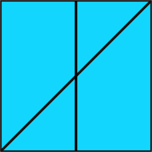
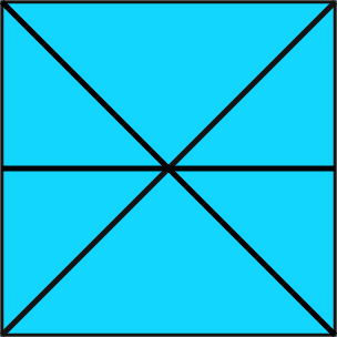
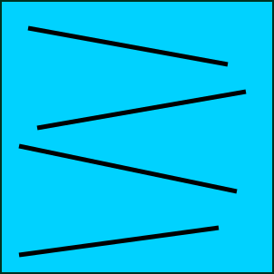
Figure 1. Examples of plates reinforced by beams.

In [11] we proposed to use the same finite element space for the beam as for the higher dimensional structure; more precisely, the trial and test space for the beam is obtained by taking the restriction or trace to the beam. Here we further develop this approach to allow for coupling between plates and beams, more precisely the Kirchhoff-Love plate model and the Bernoulli beam model. These models involve fourth order partial differential equations. We discretize these models using the so called continuous/discontinuous Galerkin, c/dG, method which relaxes the required $C^{1}$ continuity of the shape functions for the beam and plate by use of a discontinuous Galerkin approach with $C^{0}$–continuity. We emphasise that the concept is quite general, as illustrated in our previous work on embedding in elastic solids, of membranes [4] and of embedded trusses and beams [11]. A similar approach was recently suggested for modelling embedded trusses by Lé, Legrain, and Moës [12].

2. Modeling of Reinforced Plates

2.1. The Basic Approach

In this Section we develop a simple model of a set of beam elements in a plate. The main approach is as follows:

• Given a continuous finite element space, based on at least second order polynomials for the plate, we define the finite element space for the one–dimensional structure as the restriction of the plate finite element space to the structure which is geometrically modeled by an embedded curve or line.

• To formulate a finite element method on the restricted or trace finite element space we employ continuous/discontinuous Galerkin approximations of the Euler–Bernoulli beam model. The beams are then modeled using the CutFEM paradigm and the stiffness of the embedded beams is in the most basic version, which we consider here, simply added to the plate stiffness.

To ensure coercivity of the cut beam model we in general need to add a certain stabilization term which provides control of the discrete functions variation in the vicinity of the beam. However, for beams embedded in a plate, the plate stabilizes the beam discretizations, and we shall show that if the plate is stiff enough compared to the beam the usual additional stabilization [1] is superfluous. The plate problem may also be viewed as an interface problem in order to more accurately approximate the plate in the vicinity of the beam structure; this approach is however significantly more demanding from an implementation point of view and we leave it for future work.

The work presented here is an extension of earlier work [4] where membrane structures were considered, in which case a linear approximation in the bulk suffices.

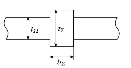
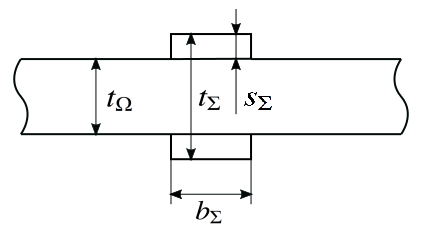
Figure 2. Left: The reinforced plate geometry parameters, $t_{\Omega}$, $t_{\Sigma}$, and $b_{\Sigma}$. Right: Alternative design of reinforcement with two separate beams of thickness $s_{\Sigma}=(t_{\Sigma}-t_{\Omega})/2$ above and below the plate.

2.2. The Kirchhoff–Love Plate Model

In the Kirchhoff–Love plate model, posed on a polygonal domain $\Omega\subset{\mathbb{R}}^{2}$ with boundary $\partial\Omega$ and exterior unit normal ${\boldsymbol{n}}$, we seek an out–of–plane (scalar) displacement $u$ to which we associate the strain (curvature) tensor

(1) $${\boldsymbol{\varepsilon}}(\nabla u):=\frac{1}{2}\left(\nabla\otimes(\nabla u)+(\nabla u)\otimes\nabla\right)=\nabla\otimes\nabla u=\nabla^{2}u$$

and the plate stress (moment) tensor

(2) $${\boldsymbol{\sigma}}_{P}(\nabla u) :=\mathcal{C}_{P}\left({\boldsymbol{\varepsilon}}(\nabla u)+\nu_{\Omega}(1-{\nu_{\Omega}})^{-1}\text{div$\,$}\nabla u\,{\boldsymbol{I}}\right)$$

(3) $$=\mathcal{C}_{P}\left(\nabla^{2}u+\nu_{\Omega}(1-\nu_{\Omega})^{-1}\Delta u{\boldsymbol{I}}\right)$$

where

(4) $$\mathcal{C}_{P}=\frac{E_{\Omega}t_{\Omega}^{3}}{12(1+\nu_{\Omega})}$$

with $E_{\Omega}$ the Young’s modulus, $\nu_{\Omega}$ the Poisson’s ratio, and $t_{\Omega}$ denotes the plate thickness. Since $0\leq\nu_{\Omega}\leq 0.5$ the constants are uniformly bounded.

The Kirchhoff–Love problem then takes the form: given the out–of–plane load (per unit area) $f$, find the displacement $u$ such that

(5) $$\text{div$\,$}\text{{\bf div}$\,$}{\boldsymbol{\sigma}}_{P}(\nabla u)=f \Omega$$ in

(6) $$u=0 \partial\Omega$$ on

(7) $${\boldsymbol{n}}\cdot\nabla u=0 \partial\Omega$$ on

where div  and div denote the divergence of a tensor and a vector field, respectively.

Weak Form

The variational problem takes the form: Find the displacement $u\in V_{\Omega}=H^{2}_{0}(\Omega)$ such that

(8) $$a_{\Omega}(u,v)=l_{\Omega}(v)\qquad\forall v\in V_{\Omega}$$

where the forms are defined by

(9) $$a_{\Omega}(v,w) =({\boldsymbol{\sigma}}_{P}(\nabla v),{\boldsymbol{\varepsilon}}(\nabla w))_{\Omega}$$

(10) $$l_{\Omega}(v) =(f,v)_{\Omega}$$

We employ the following notation: $L^{2}(\omega)$ is the Lebesgue space of square integrable functions on $\omega$ with scalar product $(\cdot,\cdot)_{L^{2}(\omega)}=(\cdot,\cdot)_{\omega}$ and $(\cdot,\cdot)_{L^{2}(\Omega)}=(\cdot,\cdot)$, and norm $\|\cdot\|_{L^{2}(\omega)}=\|\cdot\|_{\omega}$ and $\|\cdot\|_{L^{2}(\Omega)}=\|\cdot\|$, $H^{s}(\omega)$ is the Sobolev space of order $s$ on $\omega$ with norm $\|\cdot\|_{H^{s}(\omega)}$, and $H^{1}_{0}(\Omega)=\{v\in\text{$H^{1}(\Omega):$}\;v=0\text{ on $\partial\Omega$}\}$, and $H^{2}_{0}(\Omega)=\{v\in H^{2}(\Omega):\,v={\boldsymbol{n}}\cdot\nabla v=0\text{ on $\partial\Omega$}\}$.

2.3. The Euler–Bernoulli Beam Model

Consider a straight thin beam with centerline $\Sigma\subset\Omega$ and a rectangular cross-section with width $b_{\Sigma}$ and thickness $t_{\Sigma}$, see Figure 2. The modeling of the beam is performed using tangential differential calculus and we follow the exposition in [10, 11], which also covers curved beams. Using this approach the beam equation is expressed in the same coordinate system as the plate, which is convenient in the construction of the cut finite element method for reinforced plates.

Let ${\boldsymbol{t}}$ be the tangent vector to the line $\Sigma$, embedded in ${\mathbb{R}}^{2}$. We let ${\boldsymbol{p}}:\mathbb{R}^{2}\rightarrow\Sigma$ be the closest point mapping, i.e. ${\boldsymbol{p}}({\boldsymbol{x}})={\boldsymbol{y}}$ where ${\boldsymbol{y}}\in\Sigma$ minimizes the Euclidean norm $|{\boldsymbol{x}}-{\boldsymbol{y}}|_{{\mathbb{R}}^{3}}$. We define $\zeta$ as the signed distance function $\zeta({\boldsymbol{x}}):=\pm|{\boldsymbol{x}}-{\boldsymbol{p}}({\boldsymbol{x}})|$, positive on one side of $\Sigma$ and negative on the other.

Let ${\boldsymbol{P}}_{\Sigma}={\boldsymbol{t}}\otimes{\boldsymbol{t}}$ be the projection onto the one dimensional tangent space of $\Sigma$ and define the tangential derivatives

(11) $$\nabla_{\Sigma}v={\boldsymbol{P}}_{\Sigma}\nabla v,\qquad\partial_{{\boldsymbol{t}}}v={\boldsymbol{t}}\cdot\nabla v$$

Then we have the identity

(12) $$\nabla_{\Sigma}v=(\partial_{{\boldsymbol{t}}}v){\boldsymbol{t}}$$

Based on the assumption that planar cross sections orthogonal to the midline remain plane after deformation we assume that the displacement takes the form

(13) $${\boldsymbol{u}}=u{\boldsymbol{n}}+\theta\zeta{\boldsymbol{t}}$$

where $\theta:\Sigma\rightarrow\mathbb{R}$ is an angle representing an infinitesimal rotation, assumed constant in the normal plane. In Euler–Bernoulli beam theory the beam cross-section is assumed plane and orthogonal to the beam midline after deformation and no shear deformations occur, which means that we have

(14) $$\theta={\boldsymbol{t}}\cdot\nabla u:=\partial_{{\boldsymbol{t}}}u$$

This definition for $\theta$ in combination with (13) constitutes the Euler–Bernoulli kinematic assumption

$${\boldsymbol{u}}=u{\boldsymbol{n}}+\zeta(\partial_{{\boldsymbol{t}}}u){\boldsymbol{t}}=u{\boldsymbol{n}}+\zeta\nabla_{\Sigma}u$$

We assume the usual Hooke’s law for one dimensional structural members

(15) $${\boldsymbol{\sigma}}_{\Sigma}({\boldsymbol{u}})=E_{\Sigma}{\boldsymbol{\varepsilon}}_{\Sigma}({\boldsymbol{u}})$$

where $E_{\Sigma}$ is the Young modulus and the tangential strain tensor is given by

(16) $${\boldsymbol{\varepsilon}}_{\Sigma}({\boldsymbol{u}})={\boldsymbol{P}}_{\Sigma}{\boldsymbol{\varepsilon}}({\boldsymbol{u}}){\boldsymbol{P}}_{\Sigma}=\zeta{\boldsymbol{\varepsilon}}_{\Sigma}(\nabla_{\Sigma}u)$$

where in the last equality we used the identity

(17) $${\boldsymbol{u}}\otimes\nabla=(u{\boldsymbol{n}}+\zeta\nabla_{\Sigma}u)\otimes\nabla={\boldsymbol{n}}\otimes(\nabla u)+\zeta(\nabla_{\Sigma}u)\otimes\nabla$$

to conclude that

(18) $${\boldsymbol{\varepsilon}}_{\Sigma}({\boldsymbol{u}})=\zeta{\boldsymbol{\varepsilon}}_{\Sigma}(\nabla_{\Sigma}u)$$

Next note that the strain energy density can be written

(19) $${\boldsymbol{\sigma}}_{\Sigma}({\boldsymbol{u}}):{\boldsymbol{\varepsilon}}_{\Sigma}({\boldsymbol{u}})=\zeta^{2}{\boldsymbol{\sigma}}_{\Sigma}(\nabla_{\Sigma}u):{\boldsymbol{\varepsilon}}(\nabla_{\Sigma}u)$$

and the total energy of the beam structure is obtained by integrating over the beam volume

(20) $${\mathcal{E}}_{\Sigma}=\frac{1}{2}\int_{\Sigma}I_{\Sigma}{\boldsymbol{\sigma}}_{\Sigma}(\nabla_{\Sigma}u):{\boldsymbol{\varepsilon}}(\nabla_{\Sigma}u)\,d\Sigma-\int_{\Sigma}a_{\Sigma}f_{\Sigma}u\,d\Sigma$$

where the integral over the cross section is accounted for by the cross-section area and its second moment

(21) $$a_{\Sigma}=b_{\Sigma}t_{\Sigma},\qquad I_{\Sigma}=b_{\Sigma}t_{\Sigma}^{3}/12$$

We are thus led to introducing the beam stress tensor

(22) $${\boldsymbol{\sigma}}_{B,\Sigma}(\nabla_{\Sigma}v)=I_{\Sigma}{\boldsymbol{\sigma}}_{\Sigma}(\nabla_{\Sigma}v)=I_{\Sigma}E_{\Sigma}{\boldsymbol{\varepsilon}}_{\Sigma}(\nabla_{\Sigma}v)$$

and thus we have the beam Hooke law

(23) $${\boldsymbol{\sigma}}_{B,\Sigma}(\nabla_{\Sigma}v)=\mathcal{C}_{B}{\boldsymbol{\varepsilon}}_{\Sigma}(\nabla_{\Sigma}v)$$

where

(24) $$\mathcal{C}_{B}=E_{\Sigma}I_{\Sigma}=\frac{E_{\Sigma}b_{\Sigma}t_{\Sigma}^{3}}{12}$$

Taking variations we obtain the weak statement, assuming zero displacements and rotations at the end points of $\Sigma$, we thus seek $u\in V_{\Sigma}=H^{2}_{0}(\Sigma)$, such that

(25) $$a_{\Sigma}(u,v)=l_{\Sigma}(v)\qquad\forall v\in V_{\Sigma}$$

where the forms are defined by

(26) $$a_{\Sigma}(v,w)=\int_{\Sigma}{\boldsymbol{\sigma}}_{B,\Sigma}(\nabla_{\Sigma}v):{\boldsymbol{\varepsilon}}_{\Sigma}(\nabla_{\Sigma}w)\,d\Sigma,\qquad l_{\Sigma}(v)=\int_{\Sigma}a_{\Sigma}f_{\Sigma}v\,d\Sigma$$

Remark 1.

We have the identity

(27) $${\boldsymbol{\varepsilon}}_{\Sigma}(\nabla_{\Sigma}v)=(\partial_{{\boldsymbol{t}}}^{2}v){\boldsymbol{t}}\otimes{\boldsymbol{t}}$$

since $(\nabla_{\Sigma}v)\otimes\nabla_{\Sigma}=((\partial_{{\boldsymbol{t}}}v){\boldsymbol{t}})\otimes\nabla_{\Sigma}=(\partial_{{\boldsymbol{t}}}(\partial_{{\boldsymbol{t}}}v){\boldsymbol{t}})\otimes{\boldsymbol{t}}=(\partial^{2}_{{\boldsymbol{t}}}v){\boldsymbol{t}}\otimes{\boldsymbol{t}}$, and thus

(28) $${\boldsymbol{\sigma}}_{B,\Sigma}(\nabla_{\Sigma}v):{\boldsymbol{\varepsilon}}(\nabla_{\Sigma}w)=E_{\Sigma}I_{\Sigma}\partial_{{\boldsymbol{t}}}^{2}v\partial_{{\boldsymbol{t}}}^{2}w$$

which leads to

(29) $$a_{\Sigma}(v,w)=\int_{\Sigma}{\boldsymbol{\sigma}}_{B,\Sigma}(\nabla_{\Sigma}v):{\boldsymbol{\varepsilon}}(\nabla_{\Sigma}w)\,d\Sigma=\int_{\Sigma}E_{\Sigma}I_{\Sigma}\partial_{{\boldsymbol{t}}}^{2}v\partial_{{\boldsymbol{t}}}^{2}w\,d\Sigma$$

Here we recognize the right hand side as the traditional bilinear form associated with the Euler-Bernoulli beam.

Remark 2.

We note that in the alternative reinforcement geometry, right in Figure 2, we have

(30) $$a_{\Sigma}=b_{\Sigma}(t_{\Sigma}-t_{\Omega}),\qquad I_{\Sigma}=\frac{E_{\Sigma}b_{\Sigma}(t^{3}_{\Sigma}-t^{3}_{\Omega})}{12}$$

We may also consider more complicated cross sections and compute the proper parameters.

2.4. The Reinforced Plate Model

Let $\mathcal{S}=\{S\}$ be a set of beams arbitrarily oriented in $\Omega$. Using superposition we obtain the problem: find $u\in V$ such that

(31) $$a(u,v)=l(v)\qquad\forall v\in V$$

where

(32) $$V=V_{\Omega}\bigcap_{\Sigma\in\mathcal{S}}V_{\Sigma}$$

and the forms are defined by

(33) $$a(v,w) =a_{\Omega}(v,w)+\sum_{\Sigma\in\mathcal{S}}a_{\Sigma}(v,w)$$

(34) $$l(v) =l_{\Omega}(v)+\sum_{\Sigma\in\mathcal{S}}l_{\Sigma}(v)$$

Remark 3.

Note that for the alternative plate reinforcement geometry, right in Figure 2, there is no geometric error in our method if we use the parameters (30). In the standard reinforcement geometry, left in Figure 2, there is a however a geometric error proportional to $b_{\Sigma}$ in the plate bilinear form, which arises in the superposition since the intersection between the beam and the plate is nonempty. We will later see that $b_{\Sigma}$ typically is smaller (in practice significantly smaller) than the mesh size since we are using thin beam and plate theory, see (35), and thus the geometric error is small.

3. Finite Element Discretization

3.1. The Mesh and Finite Element Spaces

• We consider a subdivision $\mathcal{T}_{h}=\{T\}$ of $\Omega$ into a geometrically conforming finite element mesh, with mesh parameter $h\in(0,h_{0}]$. We assume that the elements are shape regular, i.e., the quotient of the diameter of the smallest circumscribed sphere and the largest inscribed sphere is uniformly bounded. We denote by $h_{T}$ the diameter of element $T$ and by $h=\max_{T\in\mathcal{T}_{h}}h_{T}$ the global mesh size parameter.

• Since we are using thin plate and beam theory we assume that there is a constant $C_{\text{mesh}}$ such that

  (35) $$C_{\text{mesh}}\max(t_{\Omega},t_{\Sigma},b_{\Sigma})\leq h$$

• We shall use continuous, piecewise polynomial approximations, for both the membrane and plate problem. Let

  (36) $$V_{\Omega,h,k}=\{v\in C^{0}(\Omega):~{}\text{$v|_{T}\in\mathcal{P}_{k}(T)$ $\forall T\in\mathcal{T}$}\}$$

  where $\mathcal{P}_{k}(T)$ is the space of polynomials of degree less or equal to $k$ defined on $T$. For simplicity, we write $V_{\Omega,h}=V_{\Omega,h,k}$.

• To define our method we introduce the set of faces (edges) $F$ in the mesh, $\mathcal{F}_{h}=\{F\}$, and we split $\mathcal{F}_{h}$ into two disjoint subsets

  (37) $$\mathcal{F}_{h}=\mathcal{F}_{h,I}\cup\mathcal{F}_{h,B}$$

  where $\mathcal{F}_{h,I}$ is the set of faces in the interior of $\Omega$ and $\mathcal{F}_{h,B}$ is the set of faces on the boundary.

• Further, with each face $F$ we associate a fixed unit normal ${\boldsymbol{n}}_{F}$ such that for faces on the boundary ${\boldsymbol{n}}_{F}$ is the exterior unit normal. We denote the jump of a function ${\boldsymbol{v}}$ at a face $F$ by $\left[{\boldsymbol{v}}\right]={\boldsymbol{v}}^{+}-{\boldsymbol{v}}^{-}$ for $F\in\mathcal{F}_{h,I}$ and $\left[{\boldsymbol{v}}\right]={\boldsymbol{v}}^{+}$ for $F\in\mathcal{F}_{h,B}$, and the average $\langle{\boldsymbol{v}}\rangle=({\boldsymbol{v}}^{+}+{\boldsymbol{v}}^{-})/2$ for $F\in\mathcal{F}_{h,I}$ and $\langle{\boldsymbol{v}}\rangle={\boldsymbol{v}}^{+}$ for $F\in\mathcal{F}_{h,B}$, where ${\boldsymbol{v}}^{\pm}=\lim_{\epsilon\downarrow 0}{\boldsymbol{v}}({\boldsymbol{x}}\mp\epsilon\,{\boldsymbol{n}}_{F})$ with ${\boldsymbol{x}}\in F$.

• Given a line segment $\Sigma$ in $\Omega$ that represents a beam we let

  $$\mathcal{T}_{h}(\Sigma)=\{T\in\mathcal{T}_{h}:T\cap\Sigma\neq\emptyset\}$$

  and we let $\mathcal{F}_{h}(\Sigma)$ be the set of all interior faces in $\mathcal{T}_{h}(\Sigma)$.

• The intersection points between $\Sigma$ and element faces in $\mathcal{F}_{h}(\Sigma)$ is denoted

  (38) $$\mathcal{P}_{h}(\Sigma)=\{{\boldsymbol{x}}:\,{\boldsymbol{x}}=F\cap\Sigma,\,F\in\mathcal{F}_{h}(\Sigma)\}$$

  and we assume that this is a discrete set of points (thus excluding the case where any $F\in\mathcal{F}_{h}$ coincides with a part of $\Sigma$).

  

  

  

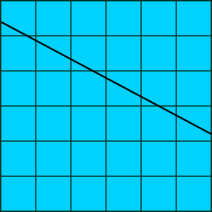
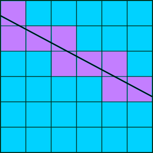
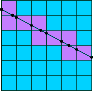
  Figure 3. The mesh $\mathcal{T}_{h}$ with one beam, the active mesh $\mathcal{T}_{h}(\Sigma)$ for the beam in purple, and the set of intersection points $\mathcal{P}_{h}(\Sigma)$.

3.2. The c/dG Method for the Plate

We approximate the solution to the plate problem using the continuous/discontinuous Galerkin (c/dG) method: Find $u_{h}\in V_{\Omega,h}$, with $k\geq 2$, such that

(39) $$a_{\Omega,h}(u_{h},v)=l_{\Omega}(v)\qquad\forall v\in V_{\Omega,h}$$

The bilinear form $a_{\Omega,h}(\cdot,\cdot)$ is defined by

(40) $$a_{\Omega,h}(v,w)={} \sum_{T\in\mathcal{T}_{h}}({\boldsymbol{\sigma}}_{P}(\nabla v),{\boldsymbol{\varepsilon}}(\nabla w))_{T}$$

$$\qquad-\sum_{F\in\mathcal{F}_{h,I}\cup\mathcal{F}_{h,B}}(\langle{\boldsymbol{n}}_{F}\cdot{\boldsymbol{\sigma}}_{P}(\nabla v)\rangle,[\nabla w])_{F}$$

$$\qquad-\sum_{F\in\mathcal{F}_{h,I}\cup\mathcal{F}_{h,B}}([\nabla v],\langle{\boldsymbol{n}}_{F}\cdot{\boldsymbol{\sigma}}_{P}(\nabla w)\rangle)_{F}$$

$$\qquad+\sum_{F\in\mathcal{F}_{h,I}\cup\mathcal{F}_{h,B}}\beta_{\Omega}h_{F}^{-1}([\nabla v],\left[\nabla w\right])_{F}$$

Here $\beta_{\Omega}$ is a positive parameter of the form

(41) $$\beta_{\Omega}=\beta_{\Omega,0}\mathcal{C}_{P}=\beta_{\Omega,0}\frac{E_{\Omega}t_{\Omega}^{3}}{12(1+\nu_{\Omega})}$$

where $\beta_{\Omega,0}$ is a constant depending on the polynomial order $k$, see [9] for details, and $h_{F}$ is defined on each face $F$ by

(42) $$h_{F}=\left(|T^{+}|+|T^{-}|\right)/(2\,|F|)\quad\text{for $F=\partial T^{+}\cap\partial T^{-}$}$$

with $|T|$ the area of $T$ and $|F|$ the length of $F$.

Remark 4.

The idea of using continuous/discontinuous approximations was first proposed by Engel et al. [5] and later analysed for Kirchhoff–Love and Mindlin–Reissner plates in [8, 9, 6], cf. also Wells and Dung [16].

Remark 5.

Other boundary conditions for plates, for instance simply supported and free, can easily be included in the c/dG finite element method, see [7] for details.

Remark 6.

For $v\in V_{\Omega,h}$ we have $[\nabla v]=[{\boldsymbol{n}}_{F}\cdot\nabla v]{\boldsymbol{n}}_{F}$ since $v$ is continuous across a face and $v=0$ on $\partial\Omega$. Therefore

(43) $$(\langle{\boldsymbol{n}}_{F}\cdot{\boldsymbol{\sigma}}(\nabla v)\rangle,[\nabla w])_{F}=(\langle{\boldsymbol{n}}_{F}\cdot{\boldsymbol{\sigma}}(\nabla v)\cdot{\boldsymbol{n}}_{F}\rangle,[{\boldsymbol{n}}_{F}\cdot\nabla w])_{F}\quad$$

for all $v,w\in V_{\Omega,h}$, and we note that $({\boldsymbol{n}}_{F}\cdot{\boldsymbol{\sigma}}(\nabla u)\cdot{\boldsymbol{n}}_{F})|_{F}$ is the bending moment at the edge $F$.

3.3. The Cut c/dG Method for a Beam

We propose the following cut c/dG method. Find $u_{h}\in V_{\Sigma,h}=V_{\Omega,h}|_{\mathcal{T}_{h}(\Sigma)}$ such that

(44) $$A_{\Sigma,h}(u_{h},v)=l_{\Sigma}(v)\qquad\forall v\in V_{\Sigma,h}$$

where

(45) $$A_{\Sigma,h}(v,w) =a_{\Sigma,h}(v,w)+s_{\Sigma,h}(v,w)$$

(46) $$a_{\Sigma,h}(v,w) =\sum_{T\in\mathcal{T}_{h}(\Sigma)}({\boldsymbol{\sigma}}_{B,\Sigma}(\nabla_{\Sigma}v),{\boldsymbol{\varepsilon}}(\nabla_{\Sigma}w))_{\Sigma\cap T}$$

$$\qquad-\sum_{{\boldsymbol{x}}\in\mathcal{P}_{h}(\Sigma)}(\langle{\boldsymbol{t}}\cdot{\boldsymbol{\sigma}}_{B,\Sigma}(\nabla_{\Sigma}v)\rangle,[\nabla_{\Sigma}w])_{\boldsymbol{x}}$$

$$\qquad-\sum_{{\boldsymbol{x}}\in\mathcal{P}_{h}(\Sigma)}([\nabla_{\Sigma}v]{\color[rgb]{0,0,0},}\langle{\boldsymbol{t}}\cdot{\boldsymbol{\sigma}}_{B,\Sigma}(\nabla_{\Sigma}w),\rangle)_{\boldsymbol{x}}$$

$$\qquad+\sum_{{\boldsymbol{x}}\in\mathcal{P}_{h}(\Sigma)}\beta_{\Sigma,z}([\nabla_{\Sigma}v],[\nabla_{\Sigma}w])_{{\boldsymbol{x}}}$$

(47) $$s_{\Sigma,h}(v,w) =\sum_{F\in\mathcal{F}_{h,I}(\Sigma)}\sum_{j=1}^{k}\gamma_{\Sigma,1}h^{2(j-2)}([\partial^{j}_{{\boldsymbol{n}}_{F}}v],[\partial^{j}_{{\boldsymbol{n}}_{F}}w])_{F}$$

$$\qquad+\sum_{T\in\mathcal{T}_{h,I}(\Sigma)}\sum_{j=0}^{2}\gamma_{\Sigma,2}h^{2(j-2)+1}(\partial_{{\boldsymbol{n}}_{\Sigma}}\partial^{j}_{{\boldsymbol{t}}}v,\partial_{{\boldsymbol{n}}_{\Sigma}}\partial^{j}_{{\boldsymbol{t}}}w)_{T}$$

the penalty parameter takes the form

(48) $$\beta_{\Sigma}=\beta_{\Sigma,0}\mathcal{C}_{B}=\beta_{\Sigma,0}{E_{\Sigma}I_{\Sigma}}$$

with $\beta_{\Sigma,0}$ a parameter that only depends on the polynomial order, and $s_{h}$, with positive parameters $\gamma_{\Sigma,i}$, is a stabilization term which is added to ensure coercivity and stability of the stiffness matrix, cf. [1].

Remark 7.

Using the identities

(49) $$\nabla_{\Sigma}v=(\partial_{{\boldsymbol{t}}}v){\boldsymbol{t}},\qquad{\boldsymbol{\varepsilon}}_{\Sigma}(\nabla_{\Sigma}v)=(\partial_{{\boldsymbol{t}}}^{2}v){\boldsymbol{t}}\otimes{\boldsymbol{t}},\qquad{\boldsymbol{\sigma}}_{B,\Sigma}(\nabla_{\Sigma}v)=E_{\Sigma}I_{\Sigma}(\partial_{{\boldsymbol{t}}}^{2}v){\boldsymbol{t}}\otimes{\boldsymbol{t}}$$

we note that $a_{\Sigma,h}$ can alternatively be written in the form

(50) $$a_{\Sigma,h}(v,w) =\sum_{T\in\mathcal{T}_{h}(\Sigma)}(E_{\Sigma}I_{\Sigma}\,\partial_{{\boldsymbol{t}}}^{2}v,\partial_{{\boldsymbol{t}}}^{2}w)_{\Sigma\cap T}$$

$$\qquad-\sum_{{\boldsymbol{x}}\in\mathcal{P}_{h}(\Sigma)}(\langle E_{\Sigma}I_{\Sigma}\partial_{{\boldsymbol{t}}}^{2}v\rangle,[\partial_{{\boldsymbol{t}}}w])_{{\boldsymbol{x}}}$$

$$\qquad-\sum_{{\boldsymbol{x}}\in\mathcal{P}_{h}(\Sigma)}([\partial_{{\boldsymbol{t}}}{\color[rgb]{0,0,0}v}],\langle E_{\Sigma}I_{\Sigma}\partial_{{\boldsymbol{t}}}^{2}{\color[rgb]{0,0,0}w}\rangle)_{{\boldsymbol{x}}}$$

$$\qquad+\sum_{{\boldsymbol{x}}\in\mathcal{P}_{h}(\Sigma)}\frac{\beta_{\Sigma,0}}{h}(E_{\Sigma}I_{\Sigma}[\partial_{{\boldsymbol{t}}}v],[\partial_{{\boldsymbol{t}}}w])_{{\boldsymbol{x}}}$$

which is the form in [5].

Remark 8.

The terms on the discrete set $\mathcal{P}_{h}(\Sigma)$ are associated with the work of the end moments on the end rotation which occur due to the lack of $C^{1}(\Omega)$ continuity of the approximation, as in the plate model. See Remark 6.

Remark 9.

We note that due to the stabilization this method works for a single beam, i.e. without being embedded in a plate. The basic principle is the same as for the trace finite element method proposed in [14] and the stabilized version proposed in [2]. When the beam is embedded in a plate, which is the case in this work, the need for the stabilization term is mitigated, and if the plate is sufficiently stiff we may omit the stabilization term, see Section 3.5 for further details.

3.4. The c/dG Method for the Reinforced Plate Model

Recall that $\mathcal{S}=\{\Sigma\}$ is a set of beams arbitrarily oriented in $\Omega$. Using superposition we obtain the problem: find $u_{h}\in V_{\Omega,h}$ such that

(51) $$A_{h}(u_{h},v)=l(v)\qquad\forall v\in V_{\Omega,h}$$

where the forms are defined by

(52) $$A_{h}(v,w) =a_{\Omega,h}(v,w)+\sum_{\Sigma\in\mathcal{S}}a_{\Sigma,h}(v,w)$$

(53) $$l(v) =l_{\Omega}(v)+\sum_{\Sigma\in\mathcal{S}}l_{\Sigma}(v)$$

3.5. Coercivity for Reinforced Plates

In this section we study the coercivity of the c/dG method for the reinforced plate. We shall use the stability provided by the plate to prove stability of the reinforced plate, without the need of the stabilizing terms ($\gamma_{\Sigma,1}=\gamma_{\Sigma,2}=0$). This is only possible as long as the mesh size $h$ is larger than or equal to the beam with $b_{\Sigma}$. When this condition is not satisfied, stability uniform in $h$ is achieved only when the stabilizing terms are included ($\gamma_{\Sigma,1},\gamma_{\Sigma,2}>0$), using similar ideas as in [2, 3].

Coercivity of the Plate

We first recall that the c/dG method for the plate is coercive. Introducing the energy norm

(54) $$|\mspace{-1.0mu}|\mspace{-1.0mu}|v|\mspace{-1.0mu}|\mspace{-1.0mu}|^{2}_{\Omega,h}=\sum_{T\in\mathcal{T}_{h}}\mathcal{C}_{P}\|\nabla^{2}v\|^{2}_{T}+\sum_{F\in\mathcal{F}_{h}}\mathcal{C}_{P}h\|\langle\nabla^{2}v\rangle\|^{2}_{F}+\sum_{F\in\mathcal{F}_{h}}\mathcal{C}_{P}h^{-1}\|[\nabla v]\|^{2}_{F}$$

there is a constant $m_{P}>0$ such that

(55) $$m_{P}|\mspace{-1.0mu}|\mspace{-1.0mu}|v|\mspace{-1.0mu}|\mspace{-1.0mu}|^{2}_{\Omega,h}\leq a_{\Omega,h}(v,v)\qquad\forall v\in V_{\Omega,h}$$

for $\beta_{\Omega}$ large enough.

Coercivity of the Reinforced Plate

Next turning to the reinforced plate we introduce the energy norm associated with the beam

(56) $$|\mspace{-1.0mu}|\mspace{-1.0mu}|v|\mspace{-1.0mu}|\mspace{-1.0mu}|^{2}_{\Sigma,h}=\sum_{T\in\mathcal{T}_{h}(\Sigma)}\mathcal{C}_{B}\|{\color[rgb]{0,0,0}\partial_{{\boldsymbol{t}}}^{2}}v\|^{2}_{{\color[rgb]{0,0,0}\Sigma\cap T}}+\sum_{{\boldsymbol{x}}\in\mathcal{P}_{h}(\Sigma)}\mathcal{C}_{B}h\|\langle{\color[rgb]{0,0,0}\partial_{{\boldsymbol{t}}}^{2}}v\rangle\|^{2}_{{\boldsymbol{x}}}+\sum_{{\boldsymbol{x}}\in\mathcal{P}_{h}(\Sigma)}\mathcal{C}_{B}h^{-1}\|[{\color[rgb]{0,0,0}\partial_{{\boldsymbol{t}}}}v]\|^{2}_{{\boldsymbol{x}}}$$

Then there is a constant $m$ such that

(57) $$m\left(|\mspace{-1.0mu}|\mspace{-1.0mu}|v|\mspace{-1.0mu}|\mspace{-1.0mu}|^{2}_{\Sigma,h}+|\mspace{-1.0mu}|\mspace{-1.0mu}|v|\mspace{-1.0mu}|\mspace{-1.0mu}|^{2}_{\Omega,h}\right)\lesssim A_{h}(v,v)\qquad\forall v\in V_{h}$$

for $\beta_{\Omega}$ and $\beta_{\Sigma}$ large enough.

Verification of (57)

Using the following two inequalities, which we verify below,

(58) $$C_{1}\left(\sum_{{\boldsymbol{x}}\in\mathcal{P}_{h}(\Sigma)}\mathcal{C}_{B}h\|\langle{\color[rgb]{0,0,0}\partial_{{\boldsymbol{t}}}^{2}}v\rangle\|^{2}_{{\boldsymbol{x}}}\right)\leq\sum_{T\in\mathcal{T}_{h}}\mathcal{C}_{P}\|\nabla^{2}v\|^{2}_{T}$$

for some constant $C_{1}>0$, and

(59) $$\sum_{T\in\mathcal{T}_{h}(\Sigma)}\mathcal{C}_{B}\|\partial^{2}_{{\boldsymbol{t}}}v\|^{2}_{\Sigma\cap T}+\sum_{{\boldsymbol{x}}\in\mathcal{P}_{h}(\Sigma)}\mathcal{C}_{B}h^{-1}\|[\partial_{{\boldsymbol{t}}}v]\|^{2}_{{\boldsymbol{x}}}\leq\sum_{T\in\mathcal{T}_{h}}\frac{m_{P}}{3}\mathcal{C}_{P}\|\nabla^{2}v\|^{2}_{T}+a_{\Sigma,h}(v,v)$$

for $\beta_{\Sigma}$ large enough, we have

(60) $$A_{h}(v,v) =a_{\Omega,h}(v,v)+a_{\Sigma,h}(v,v)$$

(61) $$\geq m_{P}|\mspace{-1.0mu}|\mspace{-1.0mu}|v|\mspace{-1.0mu}|\mspace{-1.0mu}|^{2}_{\Omega,h}+a_{\Sigma,h}(v,v)$$

(62) $$=\frac{m_{P}}{3}|\mspace{-1.0mu}|\mspace{-1.0mu}|v|\mspace{-1.0mu}|\mspace{-1.0mu}|^{2}_{\Omega,h}+\frac{m_{P}}{3}|\mspace{-1.0mu}|\mspace{-1.0mu}|v|\mspace{-1.0mu}|\mspace{-1.0mu}|^{2}_{\Omega,h}+\left(\frac{m_{P}}{3}|\mspace{-1.0mu}|\mspace{-1.0mu}|v|\mspace{-1.0mu}|\mspace{-1.0mu}|^{2}_{\Omega,h}+a_{\Sigma,h}(v,v)\right)$$

(63) $$\geq\frac{m_{P}}{3}|\mspace{-1.0mu}|\mspace{-1.0mu}|v|\mspace{-1.0mu}|\mspace{-1.0mu}|^{2}_{\Omega,h}+\frac{C_{1}m_{P}}{3}{\color[rgb]{0,0,0}\left(\sum_{{\boldsymbol{x}}\in\mathcal{P}_{h}(\Sigma)}\mathcal{C}_{B}h\|\langle\partial_{{\boldsymbol{t}}}^{2}v\rangle\|^{2}_{{\boldsymbol{x}}}\right)}$$

$$\qquad+\left(\sum_{T\in\mathcal{T}_{h}(\Sigma)}\mathcal{C}_{B}\|\partial^{2}_{{\boldsymbol{t}}}v\|^{2}_{\Sigma\cap T}+\sum_{{\boldsymbol{x}}\in\mathcal{P}_{h}(\Sigma)}\mathcal{C}_{B}h^{-1}\|[\partial_{{\boldsymbol{t}}}v]\|^{2}_{{\boldsymbol{x}}}\right)$$

(64) $$\geq m\left(|\mspace{-1.0mu}|\mspace{-1.0mu}|v|\mspace{-1.0mu}|\mspace{-1.0mu}|^{2}_{\Sigma,h}+|\mspace{-1.0mu}|\mspace{-1.0mu}|v|\mspace{-1.0mu}|\mspace{-1.0mu}|^{2}_{\Omega,h}\right)$$

where $m=\min(m_{P}/3,C_{1}m_{P}/3,1)$.

Verification of (58)

We note that, for ${\boldsymbol{x}}\in\Sigma\cap T$, $T\in\mathcal{T}_{h}$, we have the inverse inequality

(65) $$\|\partial_{{\boldsymbol{t}}}^{2}v\|_{{\boldsymbol{x}}} \leq C_{\text{inv}}h^{-1}\|\partial_{{\boldsymbol{t}}}^{2}v\|_{T}\leq C_{\text{inv}}h^{-1}\|\nabla^{2}v\|_{T}$$

Using (65) we obtain, with $\mathcal{T}_{h}({\boldsymbol{x}})=\{T\in\mathcal{T}_{h}:{\boldsymbol{x}}\in\overline{T}\}$,

(66) $$\sum_{{\boldsymbol{x}}\in\mathcal{P}_{h}(\Sigma)}\mathcal{C}_{B}h\|\langle{\color[rgb]{0,0,0}\partial_{{\boldsymbol{t}}}^{2}}v\rangle\|^{2}_{{\boldsymbol{x}}} \leq\sum_{{\boldsymbol{x}}\in\mathcal{P}_{h}(\Sigma)}C^{2}_{\text{inv}}\frac{\mathcal{C}_{B}}{\mathcal{C}_{P}h}\mathcal{C}_{P}\|\nabla^{2}v\|^{2}_{\mathcal{T}_{h}({\boldsymbol{x}})}$$

(67) $$\leq C^{2}_{\text{inv}}\frac{\mathcal{C}_{B}}{\mathcal{C}_{P}h}|\mspace{-1.0mu}|\mspace{-1.0mu}|v|\mspace{-1.0mu}|\mspace{-1.0mu}|^{2}_{{\color[rgb]{0,0,0}\Omega,h}}$$

and thus we have the estimate

(68) $$\underbrace{\frac{1}{C^{2}_{\text{inv}}}\frac{\mathcal{C}_{P}h}{\mathcal{C}_{B}}}_{C_{1}}\left(\sum_{{\boldsymbol{x}}\in\mathcal{P}_{h}(\Sigma)}\mathcal{C}_{B}h\|\langle{\color[rgb]{0,0,0}\partial_{{\boldsymbol{t}}}^{2}}v\rangle\|^{2}_{{\boldsymbol{x}}}\right)\leq|\mspace{-1.0mu}|\mspace{-1.0mu}|v|\mspace{-1.0mu}|\mspace{-1.0mu}|^{2}_{{\color[rgb]{0,0,0}\Omega,h}}$$

We note, using the definitions (4) and (24) of $\mathcal{C}_{P}$ and $\mathcal{C}_{B}$, that

(69) $$\frac{\mathcal{C}_{P}h}{\mathcal{C}_{B}}=\frac{1}{1+\nu_{\Omega}}\frac{E_{\Omega}t_{\Omega}^{3}}{E_{\Sigma}t_{\Sigma}^{3}}\frac{h}{b_{\Sigma}}\geq\frac{1}{1+\nu_{\Omega}}\frac{E_{\Omega}t_{\Omega}^{3}}{E_{\Sigma}t_{\Sigma}^{3}}C_{\text{mesh}}$$

where we used the condition that the beam width is smaller than the mesh size (35) and thus the right hand side is a positive constant independent of the mesh size and so is $C_{1}$.

Verification of (59)

First we have the equality

(70) $$a_{\Sigma,h}(v,v) {\color[rgb]{0,0,0}=}\sum_{T\in\mathcal{T}_{h}(\Sigma)}\mathcal{C}_{B}\|\partial^{2}_{{\boldsymbol{t}}}v\|^{2}_{\Sigma\cap T}$$

$$\qquad-{\color[rgb]{0,0,0}2}\underbrace{\sum_{{\boldsymbol{x}}\in\mathcal{P}_{h}(\Sigma)}\mathcal{C}_{B}(\langle\partial^{2}_{{\boldsymbol{t}}}v\rangle,[\partial_{{\boldsymbol{t}}}v])_{\boldsymbol{x}}}_{\bigstar}$$

$$\qquad+\sum_{{\boldsymbol{x}}\in\mathcal{P}_{h}(\Sigma)}\beta_{\Sigma,0}\mathcal{C}_{B}h^{-1}\|[\partial_{{\boldsymbol{t}}}v]\|^{2}_{{\boldsymbol{x}}}$$

To estimate $\bigstar$ we employ the inverse inequality (65) as follows

(71) $$\bigstar ={\color[rgb]{0,0,0}2}\sum_{{\boldsymbol{x}}\in\mathcal{P}_{h}(\Sigma)}\mathcal{C}_{B}(\langle\partial^{2}_{{\boldsymbol{t}}}v\rangle,[\partial_{{\boldsymbol{t}}}v])_{\boldsymbol{x}}$$

(72) $$\leq{\color[rgb]{0,0,0}2}\sum_{{\boldsymbol{x}}\in\mathcal{P}_{h}(\Sigma)}\mathcal{C}_{B}C_{\text{inv}}h^{-1}\|\nabla^{2}v\|_{\mathcal{T}_{h}({\boldsymbol{x}})}\|[\partial_{{\boldsymbol{t}}}v]\|_{{\boldsymbol{x}}}$$

(73) $$\leq\sum_{T\in\mathcal{T}_{h}(\Sigma)}\delta\mathcal{C}_{B}C_{\text{inv}}^{2}h^{-1}\|\nabla^{2}v\|^{2}_{T}$$

$$\qquad+\sum_{{\boldsymbol{x}}\in\mathcal{P}_{h}(\Sigma)}\delta^{-1}\mathcal{C}_{B}h^{-1}\|[\partial_{{\boldsymbol{t}}}v]\|^{2}_{{\boldsymbol{x}}}$$

where we used the inequality $ab\leq(\delta a^{2}+\delta^{-1}b^{2})/2$ for $\delta>0$. We then obtain (59) as follows

(74) $$\sum_{T\in\mathcal{T}_{h}}\frac{m_{P}}{3}\mathcal{C}_{P}\|\nabla^{2}v\|^{2}_{T}+a_{\Sigma,h}(v,v) \geq\sum_{T\in\mathcal{T}_{h}(\Sigma)}\mathcal{C}_{B}\|\partial^{2}_{{\boldsymbol{t}}}v\|^{2}_{\Sigma\cap T}$$

$$\qquad+\sum_{T\in\mathcal{T}_{h}}\underbrace{(\frac{m_{P}}{3}\mathcal{C}_{P}-\delta\mathcal{C}_{B}C_{\text{inv}}^{2}h^{-1})}_{\geq 0}\|\nabla^{2}v\|^{2}_{T}$$

$$\qquad+\sum_{{\boldsymbol{x}}\in\mathcal{P}_{h}(\Sigma)}\underbrace{(\beta_{\Sigma,0}-\delta^{-1})}_{\geq 1}\mathcal{C}_{B}h^{-1}\|[\partial_{{\boldsymbol{t}}}v]\|^{2}_{{\boldsymbol{x}}}$$

(75) $$\geq\sum_{{\boldsymbol{x}}\in\mathcal{P}_{h}(\Sigma)}\mathcal{C}_{B}h^{-1}\|[\partial_{{\boldsymbol{t}}}v]\|^{2}_{{\boldsymbol{x}}}+\sum_{{\boldsymbol{x}}\in\mathcal{P}_{h}(\Sigma)}\mathcal{C}_{B}h^{-1}\|[\partial_{{\boldsymbol{t}}}v]\|^{2}_{{\boldsymbol{x}}}$$

Here we choose: $\delta$ small enough to guarantee that

(76) $$0\leq\frac{m_{P}}{3}\mathcal{C}_{P}-\delta\mathcal{C}_{B}C^{2}_{\text{inv}}h^{-1}=\frac{m_{P}}{3}\mathcal{C}_{P}\left(1-\delta\frac{3}{m_{P}}\frac{\mathcal{C}_{B}C^{2}_{\text{inv}}}{\mathcal{C}_{P}h}\right)=\frac{m_{P}}{3}\mathcal{C}_{P}\left(1-\delta\frac{3}{m_{P}}\frac{1}{C_{1}}\right)$$

where as above, see (69), $C_{1}>0$ independent of the mesh parameter $h$, and $\beta_{\Sigma}$ such that

(77) $$\beta_{\Sigma}-\frac{1}{\delta}\geq 1$$

4. Numerical Examples

In this Section, we give some elementary examples of what can be achieved with the presented technique. In all numerical examples we use polynomial order $2$, $f_{\Sigma}=0$, and

$$f_{\Omega}=8{\color[rgb]{0,0,0}\mathcal{C}_{P}}(3(x^{2}(1-x)^{2}+y^{2}(1-y)^{2})+(1-6x(1-x))(1-6y(1-y)))$$

corresponding to the solution $u=x^{2}(1-x)^{2}y^{2}(1-y)^{2}$ for a clamped plate unsupported by beams.

In order to handle more general boundary conditions we in particular need to be able to impose end displacements on the beam in the case of a free plate (we note that strongly imposed boundary conditions on the plate are also enforced on the beam). Zero displacement of the beam endpoints ${\boldsymbol{x}}_{E}$ are imposed by adding penalty terms

(78) $$\frac{\tilde{\beta}_{\Sigma,0}}{h^{3}}(E_{\Sigma}I_{\Sigma}v,w)_{{\boldsymbol{x}}_{E}}$$

to the form $a_{\Sigma,h}(v,w)$ in (50), where $\tilde{\beta}_{\Sigma,0}$ is a penalty parameter. These terms suffice for optimal order convergence (of the beam approximation) in the case of second degree polynomial approximations since the shear forces required for energy consistency are third derivatives of displacements, and thus equal zero.

4.1. Simply supported plate using beams with different supports

We consider a simply supported plate on the domain $\Omega=(0,1)\times(0,1)$ with Young’s modulus $E_{\Omega}=100$, Poisson’s ratio $\nu_{\Omega}=1/2$, and thickness $t_{\Omega}=0.1$. The plate is supported by two beams oriented as in Fig. 4, one at $x=0.499$ and one at at $y=0.499$ (to avoid intersection with the mesh lines). The computational mesh is shown in Fig. 5 and in Fig.6 whe show a close-up of the intersection between the beams and the mesh.

For this problem we test two different supports for the beams: simply supported and fixed, and two different stiffnesses for the beams: $E_{\Sigma}=100E_{\Omega}$ and $E_{\Sigma}=1000E_{\Omega}$. The thickness and width of the beam are equal and the same as the thickness of the plate. In Fig. 7 we show the results using $E_{\Sigma}=100E_{\Omega}$, with simply supported and fixed supports; in Fig. 8 we give the corresponding isolines, and in Fig. 9 we show the results using $E_{\Sigma}=1000E_{\Omega}$, with simply supported and fixed supports; in Fig. 10 we give the corresponding isolines.

4.2. Plate only supported by beams

Next, we consider a plate with free boundaries, supported only by beams. All data for the plate are the same as in the previous example. The plate is supported by four beams positioned at $1/3$ and $2/3$ from each boundary as indicated in Fig. 11. The beams have the same dimension as previously, with Young’s modulus $E_{\Sigma}=100E_{\Omega}$. The computational mesh is unstructured and shown in Fig. 12.

We first consider the case when the beams are clamped at $x=1$ and free elsewhere. In Fig. 13 we see the corresponding deformation in elevation and isoline plot. Next we consider the case when all beams are clamped, Fig. 14, and simply supported, Fig.15. Note the the slight increase in central displacement for the latter.

Figure 4. Beam reinforced plate.

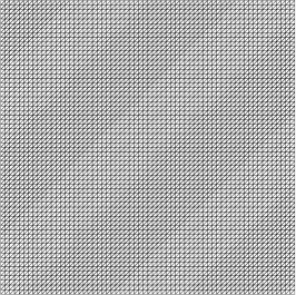
Figure 5. Computational mesh.

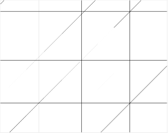
Figure 6. Beam/mesh intersection at the center.

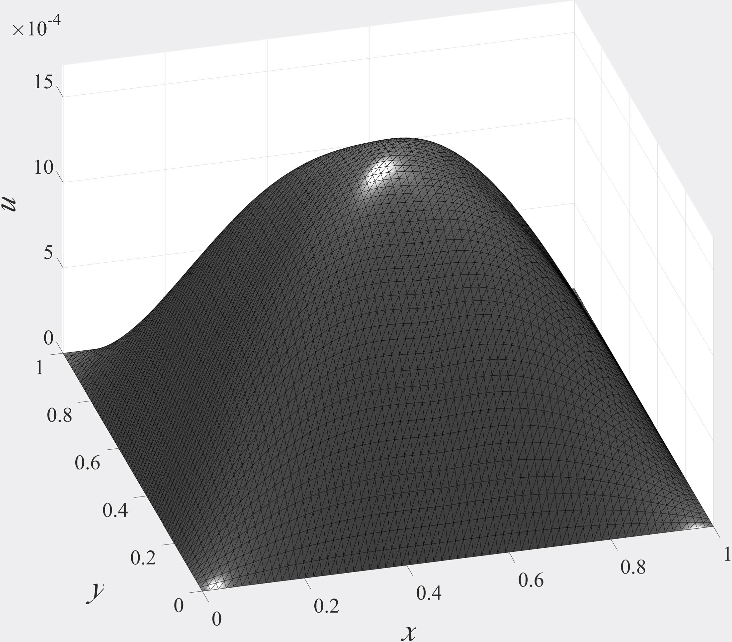
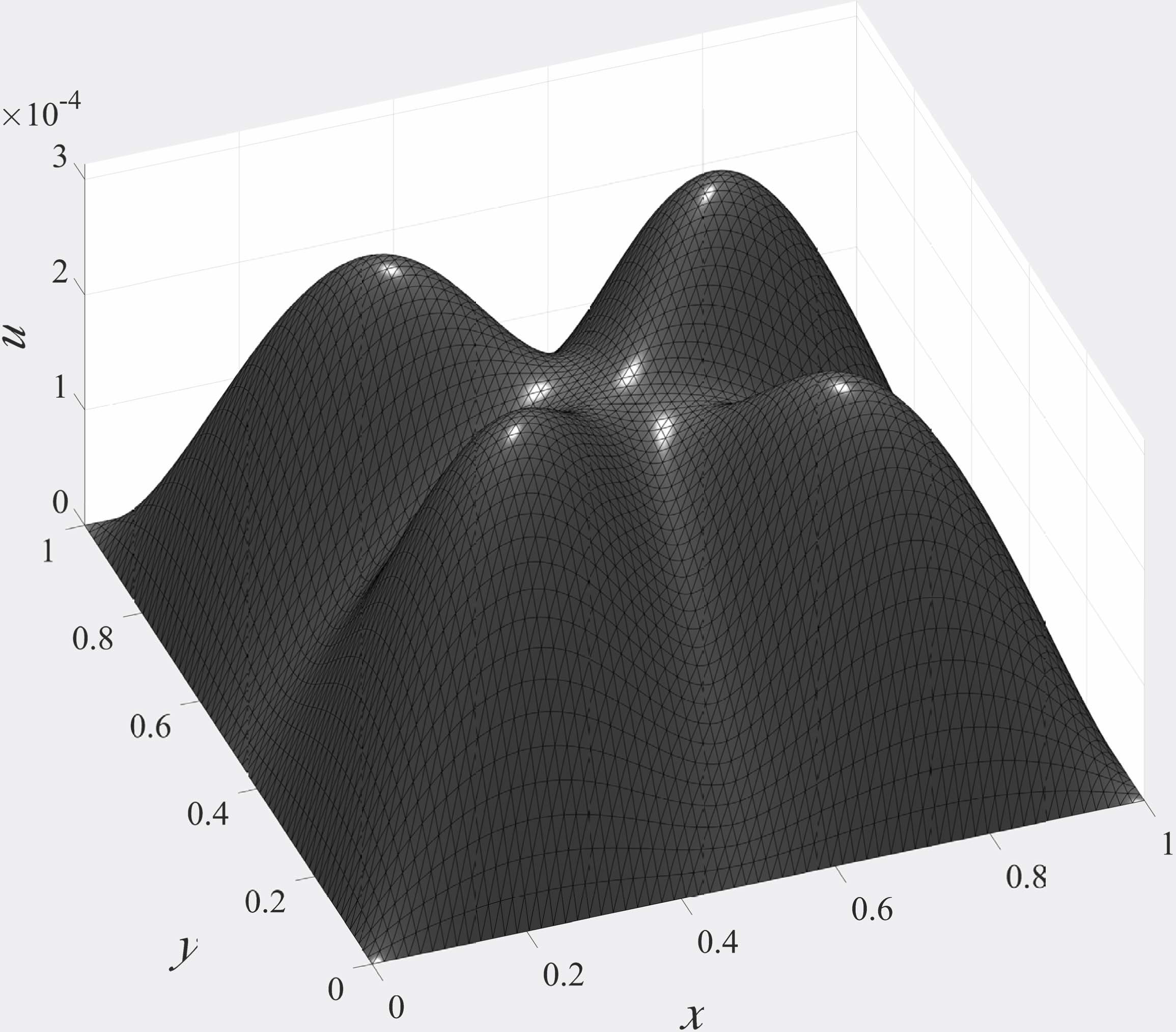
Figure 7. Displacements using simply supported support for the beams, $E_{\Sigma}=100E_{\Omega}$ (left) and $E_{\Sigma}=1000E_{\Omega}$ (right).

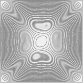
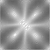
Figure 8. Isolines using simply supported beams, $E_{\Sigma}=100E_{\Omega}$ (left) and $E_{\Sigma}=1000E_{\Omega}$ (right).

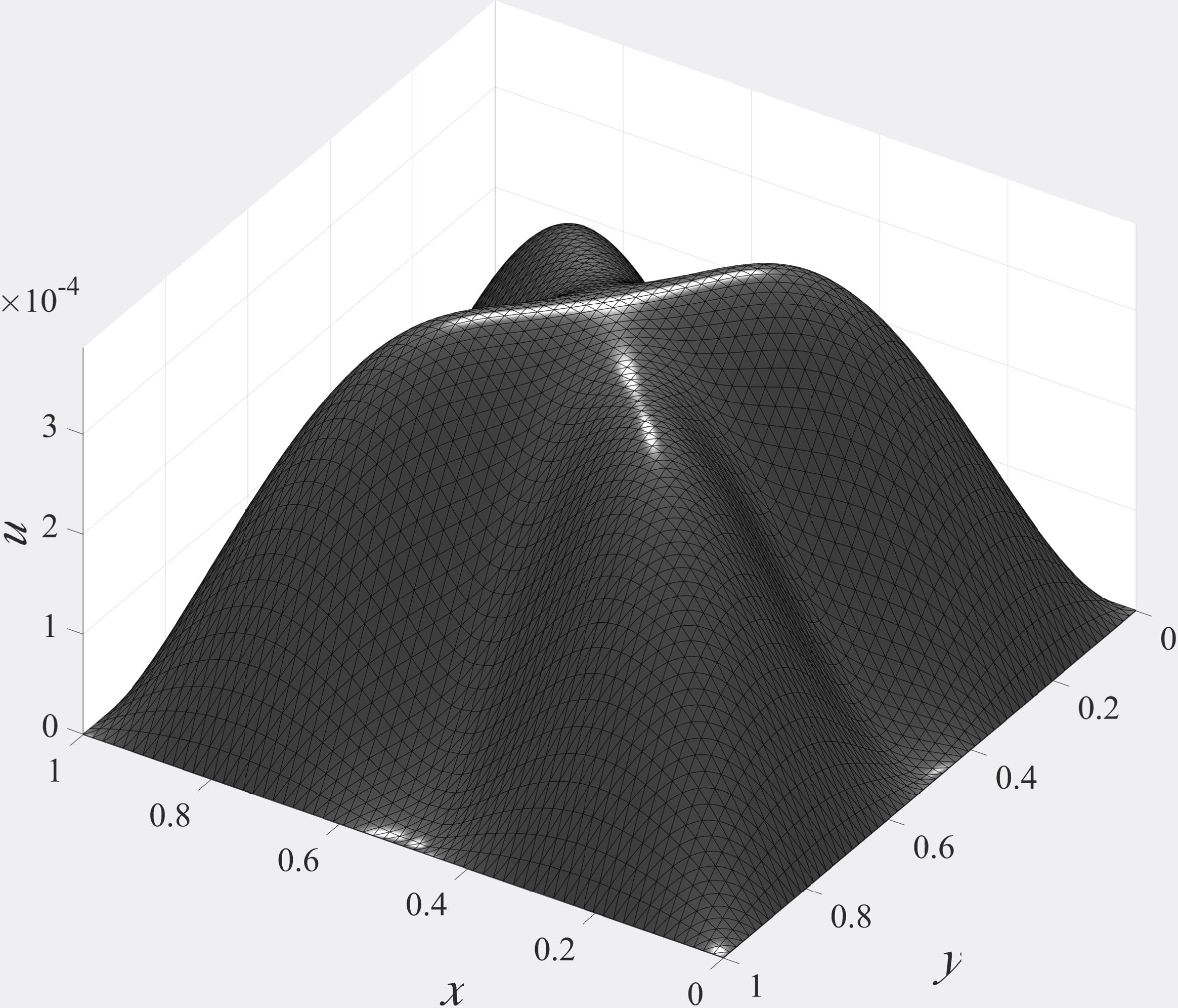
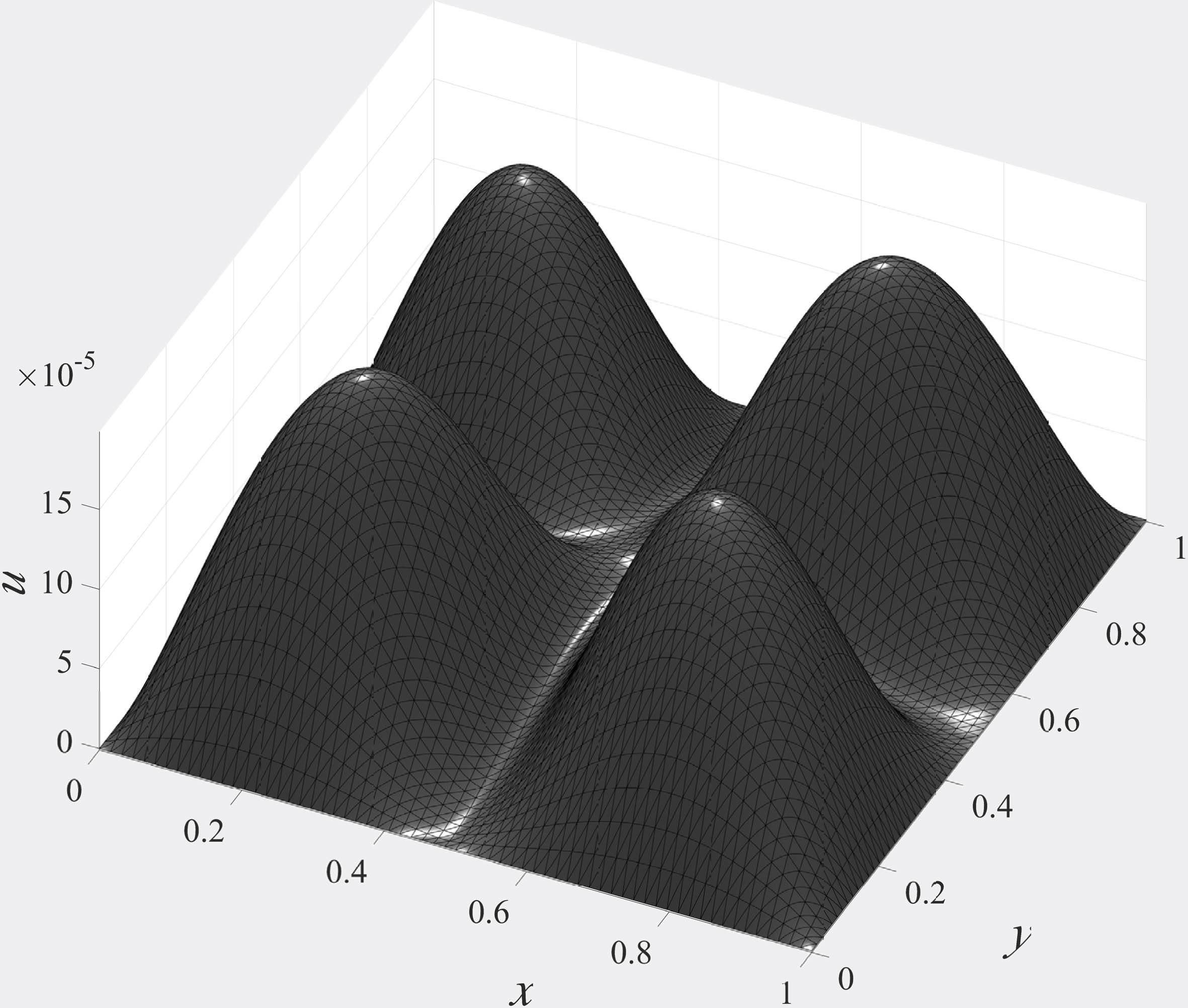
Figure 9. Displacements using fixed support for the beams, $E_{\Sigma}=100E_{\Omega}$ (left) and $E_{\Sigma}=1000E_{\Omega}$ (right).

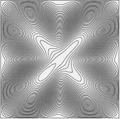
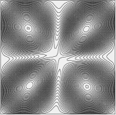
Figure 10. Isolines using fixed support for the beams, $E_{\Sigma}=100E_{\Omega}$ (left) and $E_{\Sigma}=1000E_{\Omega}$ (right).

Figure 11. Beam reinforced plate.

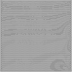
Figure 12. Computational mesh.

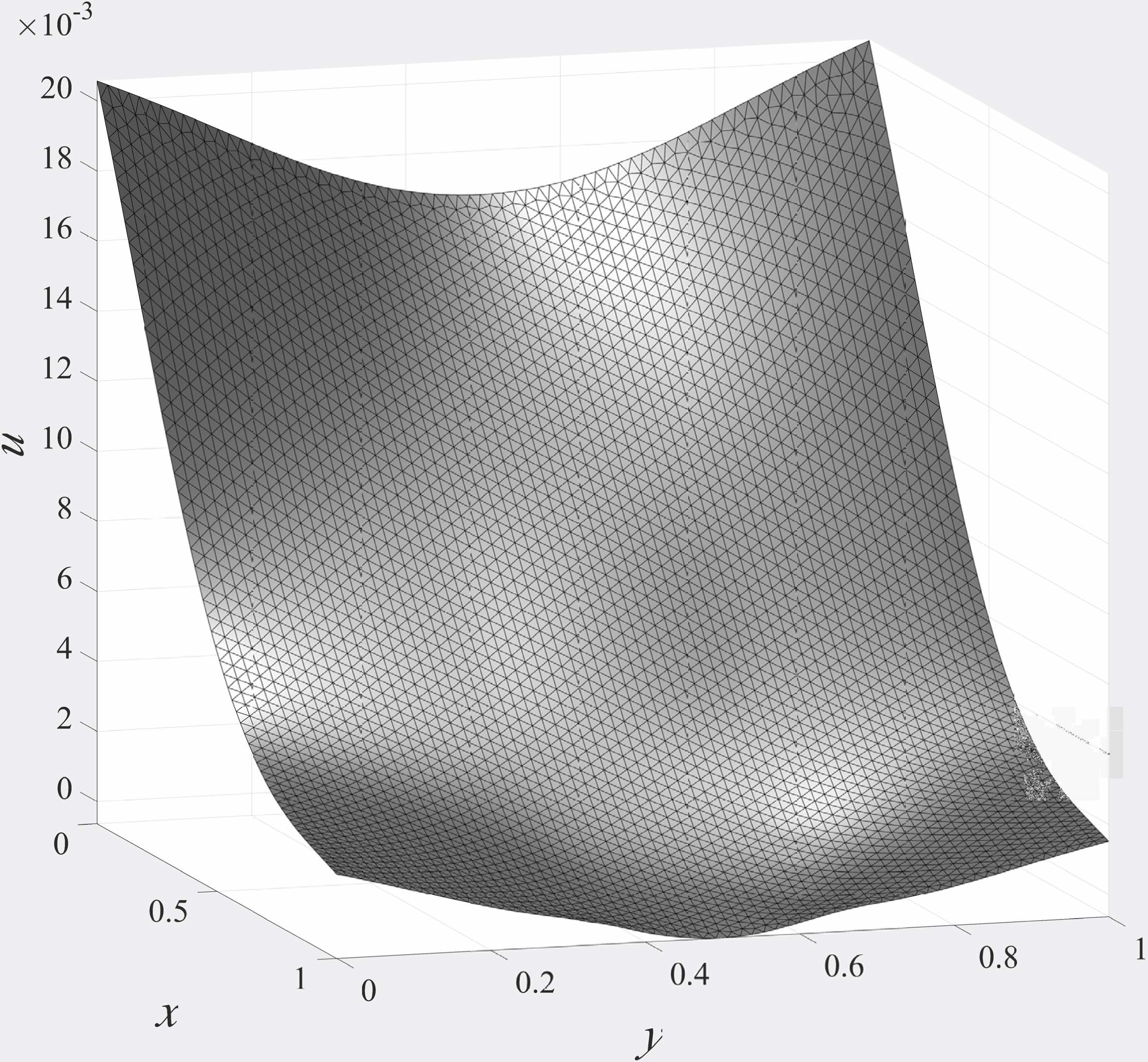
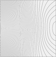
Figure 13. Deformations when the beams are clamped at $x=1$.

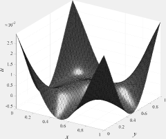
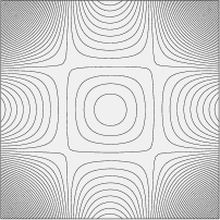
Figure 14. Deformations when all beams are clamped.

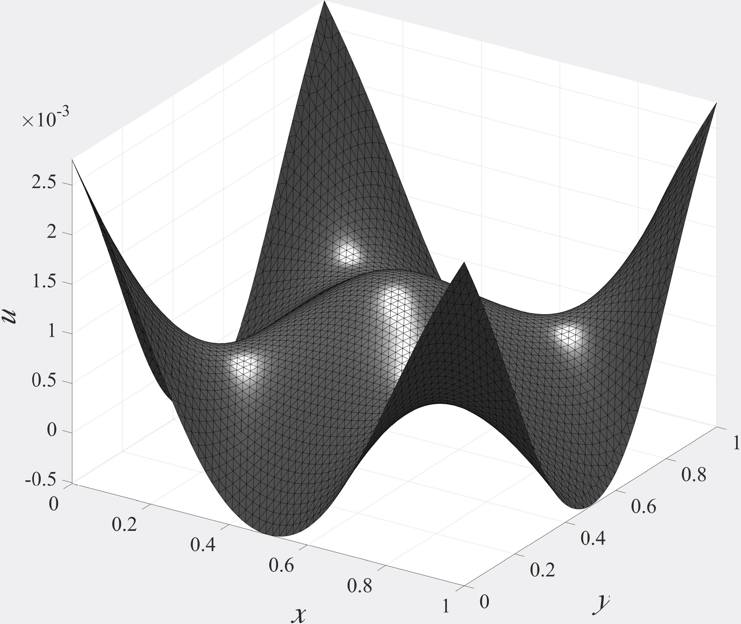
Figure 15. Deformations when all beams are simply supported.

5. Conclusions

We have formulated a continuous/discontinuous Galerkin method for beam reinforced thin plates. The method has the advantage that we can discretize both the beam and plate problem with the same standard finite element spaces of continuous piecewise polynomials defined on triangles (or quadrilaterals).

References

[1]
E. Burman, S. Claus, P. Hansbo, M. G. Larson, and A. Massing.
CutFEM: Discretizing geometry and partial differential equations.
Internat. J. Numer. Methods Engrg., 104(7):472–501, 2015.
[2]
E. Burman, P. Hansbo, and M. G. Larson.
A stabilized cut finite element method for partial differential
equations on surfaces: the Laplace-Beltrami operator.
Comput. Methods Appl. Mech. Engrg., 285:188–207, 2015.
[3]
E. Burman, P. Hansbo, M. G. Larson, and A. Massing.
Cut Finite Element Methods for Partial Differential Equations on
Embedded Manifolds of Arbitrary Codimensions.
ArXiv e-prints, Oct. 2016.
[4]
M. Cenanovic, P. Hansbo, and M. G. Larson.
Cut finite element modeling of linear membranes.
Comput. Methods Appl. Mech. Engrg., 310:98–111, 2016.
[5]
G. Engel, K. Garikipati, T. J. R. Hughes, M. G. Larson, L. Mazzei, and R. L.
Taylor.
Continuous/discontinuous finite element approximations of
fourth-order elliptic problems in structural and continuum mechanics with
applications to thin beams and plates and strain gradient elasticity.
Comput. Methods Appl. Mech. Engrg., 191(34):3669–3750, 2002.
[6]
P. Hansbo, D. Heintz, and M. G. Larson.
A finite element method with discontinuous rotations for the
Mindlin-Reissner plate model.
Comput. Methods Appl. Mech. Engrg., 200(5-8):638–648, 2011.
[7]
P. Hansbo and M. G. Larson.
A discontinuous Galerkin method for the plate equation.
Calcolo, 39(1):41–59, 2002.
[8]
P. Hansbo and M. G. Larson.
A -continuous, -discontinuous finite element method for
the Mindlin-Reissner plate model.
In Numerical mathematics and advanced applications, pages
765–774. Springer Italia, Milan, 2003.
[9]
P. Hansbo and M. G. Larson.
A posteriori error estimates for continuous/discontinuous Galerkin
approximations of the Kirchhoff-Love plate.
Comput. Methods Appl. Mech. Engrg., 200(47–48):3289–3295,
2011.
[10]
P. Hansbo, M. G. Larson, and K. Larsson.
Variational formulation of curved beams in global coordinates.
Comput. Mech., 53(4):611–623, 2014.
[11]
P. Hansbo, M. G. Larson, and K. Larsson.
Cut finite element methods for linear elasticity problems.
ArXiv e-prints, abs/1703.04377, 2017.
[12]
B. Lé, G. Legrain, and N. Moës.
Mixed dimensional modeling of reinforced structures.
Finite Elem. Anal. Des., 128:1–18, 2017.
[13]
R. McCune, C. Armstrong, and D. Robinson.
Mixed-dimensional coupling in finite element models.
Internat. J. Numer. Methods Engrg., 49(6):725–750, 2000.
[14]
M. A. Olshanskii, A. Reusken, and J. Grande.
A finite element method for elliptic equations on surfaces.
SIAM J. Numer. Anal., 47(5):3339–3358, 2009.
[15]
M. Sadek and I. Shahrour.
A three dimensional embedded beam element for reinforced
geomaterials.
Int. J. Numer. Anal. Methods Geomech., 28(9):931–946, 2004.
[16]
G. N. Wells and N. T. Dung.
A discontinuous Galerkin formulation for Kirchhoff
plates.
Comput. Methods Appl. Mech. Engrg., 196(35–36):3370–3380,
2007.