Distant entanglement enhanced in $\mathcal{PT}$-symmetric optomechanics

Abstract

We study steady-state continuous variable entanglement in a three-mode optomechanical system consisting of an active optical cavity (gain) coupled to a passive optical cavity (loss) supporting a mechanical mode. For a driving laser which is blue-detuned, we show that coupling between optical and mechanical modes is enhanced in the unbroken-$\mathcal{PT}$-symmetry regime. We analyze the stability and this shows that steady-state solutions are more stable in the gain and loss systems. We use these stable solutions to generate distant entanglement between the mechanical mode and the optical field inside the gain cavity. It results in a giant enhancement of entanglement compared to what is generated in the single lossy cavity. This work offers the prospect of exploring quantum state engineering and quantum information in such systems. Furthermore, such entanglement opens up an interesting possibility to study spatially separated quantum objects.

I Introduction

Significant advances in the study of light-matter interaction have been carried out through optomechanics [1] . Ground-state cooling of macroscopic objects [2] ; [3] ; [4] , squeezing quantum noises below the quantum standard limit [5] ; [6] , quantum entanglement [7] -[21b] , and macroscopic quantum superposition [22] have been deeply improved. This promotes a wide variety of quantum applications, such as quantum Sensors [23] , quantum informations processing [24] , quantum metrology [25] and quantum computational tasks [26] . However, there are still some limitations to fully handle certain quantum optomechanical applications and so numerous efforts are ongoing. Indeed, quantum entanglement is often limited by various factors such as the stability conditions that place constraints on the magnitude of the effective optomechanical couplings [27] -[29] and the amplification effect in the unstable regime [30] . In particular, thermal noise of the mechanical modes can strongly impair the generation of such nonclassical states.

Very recently, systems described by non-Hermitian Hamiltonians (see [31] and the references therein), have been used to engineer cavity optomechanics (COM) [32] -[36] . This has led to low-power phonon emissions [32] , emergency of chaos at low-power threshold [33] and non-reciprocal topological energy transfer [35] . These three-mode COM systems consist of an active optical cavity (gain) coupled to a passive optical cavity (loss) supporting a mechanical mode [37] -[39] . Taking advantage of the intriguing properties of these systems, we aim to improve the stability and to enhance the magnitude of the effective optomechanical couplings. Two regimes can be identified, i.e., the unbroken-$\mathcal{PT}$-symmetry regime which happens for strong optical tunneling rate and the broken-$\mathcal{PT}$-symmetry regime which happens for weak optical tunneling rate [40] . The transition between these two regimes corresponds to the exceptional point (EP). It has been shown that the intracavity photon number is significantly improved in such systems even at low driving power [32] . This leads to an enhancement of the effective optomechanical couplings. That yields a robust entanglement generation between the mechanical mode and the optical field inside the gain cavity. Furthermore, this entanglement is improved by adding a parametric amplifier (PA) in the loss cavity. It should be noted that the use of a PA for entanglement generation has been considered in [14] ; [14a] .

Our findings can be stated as follows. For a driving laser which is blue-detuned, the effective optomechanical coupling is enhanced and is more stable in the unbroken-$\mathcal{PT}$-symmetry regime. It results in a strong entanglement between the mechanical mode and the optical field inside the gain cavity. Such quantum correlation between distant modes is known as distant entanglement [41] ; [42] , and might present an interesting possibility to study spatially separated quantum objects. Our results are different from those in [41] ; [42] where the cavities that are used are lossy cavities, and therefore do not exhibit $\mathcal{PT}$-symmetry. Owing to the presence of $\mathcal{PT}$-symmetry in our configuration, the generated entanglement is enhanced compared to what is done in [41] ; [42] . Furthermore, the addition of a squeezing element in the loss cavity improves the magnitude of the effective optomechanical coupling that induces some amount of entanglement as well.

The work is organized as follows. In Sec. II, the system and the dynamical equations are described. The stability analysis is presented in Sec. III. Section IV is devoted to the continuous variable (CV) entanglement generation and their robustness against the thermal decoherence. We conclude the work in Sec. V.

II System and dynamical equations

We consider a system of two coupled microresonators (see Fig. 1), one with an optical gain $\kappa$ (active optical cavity) and the other with loss $\gamma$ (passive optical cavity) [37] -[39] . In such system, both the coupling strength $J$ and the gain-to-loss ratio of the resonators can be tuned, as experimentally demonstrated in [39] . The mechanical mode, with frequency $\omega_{m}$ and effective mass $m$, contained in the passive resonator is driven by an external field having a frequency $\omega_{p}$. The Hamiltonian of this system can be written as ($\hbar=1$) [31] ,

$$\begin{cases}H=H_{0}+H_{int},\\ H_{0}=\omega_{m}\beta^{\dagger}\beta-\Delta(\alpha_{1}^{\dagger}\alpha_{1}+\alpha_{2}^{\dagger}\alpha_{2}),\\ H_{int}=J(\alpha_{1}^{\dagger}\alpha_{2}+\alpha_{2}^{\dagger}\alpha_{1})-g\alpha_{2}^{\dagger}\alpha_{2}(\beta^{\dagger}+\beta)+\sqrt{\gamma}\epsilon^{in}(\alpha_{2}^{\dagger}+\alpha_{2}).\end{cases}$$ (1)

The lowering operators $\beta$, $\alpha_{1}$ and $\alpha_{2}$ describe the mechanical resonator, the active optical cavity and the passive optical cavity respectively. The COM coupling coefficient is given by $g$. We choose a driving pump whose frequency is blue-detuned $\Delta=\omega_{p}-\omega_{c}>0$, where $\omega_{c}$ is the cavity frequency. The Hamiltonians representing the optical gain and loss and the mechanical damping are not explicitly shown here.

From the above Hamiltonian, one derives the following set of dynamical equations,

$$\begin{cases}\dot{\alpha}_{1}=\left(i\Delta+\frac{\kappa}{2}\right)\alpha_{1}-iJ\alpha_{2}+\sqrt{\kappa}\alpha_{1}^{in},\\ \dot{\alpha}_{2}=\left[i(\Delta+g(\beta^{\dagger}+\beta))-\frac{\gamma}{2}\right]\alpha_{2}-iJ\alpha_{1}-i\sqrt{\gamma}\epsilon^{in},\\ \dot{\beta}=-(i\omega_{m}+\frac{\gamma_{m}}{2})\beta+ig\alpha_{2}^{\dagger}\alpha_{2}+\sqrt{\gamma_{m}}\beta^{in},\end{cases}$$ (2)

where $\gamma_{m}$ is the mechanical damping and $\beta^{in}$ stands for the thermal driving at finite environmental temperature $T$. The driving field $\epsilon^{in}=\alpha^{in}+\alpha_{2}^{in}$ consists of a coherent amplitude $\alpha^{in}$ and a vacuum noise operator $\alpha_{2}^{in}$. Similarly, the vacuum noise operator associated to the field $\alpha_{1}$ is $\alpha_{1}^{in}$.

In order to gain an insight into the behaviors of the system that we are interested in, namely the unbroken-$\mathcal{PT}$-symmetry and the broken-$\mathcal{PT}$-symmetry regimes, we consider only the optical modes in Eq. (2) and ignore the driving [37] . By diagonalizing these optical modes, we obtain the eigenfrequencies of the two supermodes as well as the associated linewidths as given by the real and imaginary parts, respectively, of the complex frequencies

$$\omega_{\pm}=\frac{1}{4}\left(4i\Delta-(\gamma-\kappa)\pm\sqrt{(\gamma+\kappa)^{2}-16J^{2}}\right).$$ (3)

For a strong optical tunneling rate, i.e., $J>(\gamma+\kappa)/4$, the system exhibits the purely optical unbroken-$\mathcal{PT}$-symmetry regime while the broken-$\mathcal{PT}$-symmetry regime holds for weak optical tunneling rate with $J<(\gamma+\kappa)/4$ [32] ; [40] . The transition between these two regimes, i.e., $J=(\gamma+\kappa)/4$ [32] , corresponds to the exceptional points where the two eigenfrequencies coalesce.

As the aim is to enhance entanglement, we add an additional parametric amplifier (PA) in the loss cavity as indicated in Fig. 1. This squeezing element is described by the Hamiltonian,

$$H_{\chi}=i\chi\left(e^{i\theta}(\alpha_{2}^{\dagger})^{2}-e^{-i\theta}(\alpha_{2})^{2}\right),$$ (4)

where $\chi$ is the gain of the PA while $\theta$ is the phase of the pump driving it. We have set $\theta=0$ in the whole work while the gain $\chi$ can be tuned.

In the next section, we study the stability of the steady-state solutions in order to quantify distant entanglement.

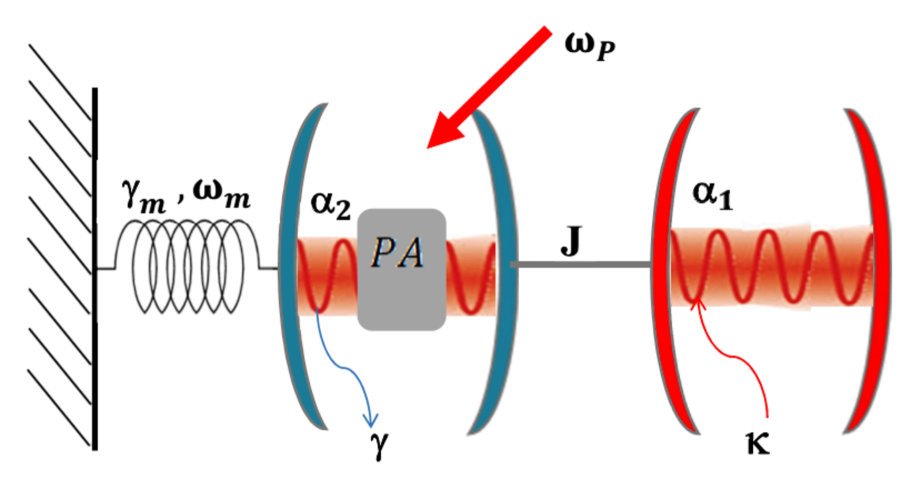
Figure 1: Setup of the gain and loss COM used. An active optical cavity (gain) is coupled to a passive optical cavity (loss) supporting a mechanical mode. A squeezing element (PA) is inserted inside the loss cavity.

III Steady states and stability analysis

For $|\langle\alpha_{2}\rangle|\gg 1$, the operators in Eq. (2) can be expanded as their mean values plus a small amount of fluctuations. This yields the steady states of our system, by linearizing the field operators around their steady-state values $\mathcal{O}(t)=O_{s}+\delta\mathcal{O}(t)$, where $\mathcal{O}\equiv(\alpha_{1}$, $\alpha_{2}$, $\beta)$. The stability analysis of these steady-state solutions should be addressed, since the important feature of these solutions is their stability. Indeed, any steady-state solution is dynamically meaningless unless it is stable. We study this stability through linear stability analysis [43] . Throughout the work, we use the following experimentally achievable parameters [37] -[39] , $\omega_{m}/2\pi=23\operatorname{MHz}$, $\gamma/2\pi=1\operatorname{MHz}$, $g=7.4\times 10^{-5}\gamma$ and $\gamma_{m}=1.63\times 10^{-3}\gamma$. The parameters $\kappa$ and $J$ will be tuned according to [39] . From the linearization, the dynamical fluctuation of the system can be described by the compact equation,

$$\dot{v}(t)=Mv(t)+z(t),$$ (5)

where $v(t)$ is the vector of the fluctuations, $v(t)=\left(\delta\beta(t),\delta\beta^{\dagger}(t),\delta\alpha_{1}(t),\delta\alpha_{1}^{\dagger}(t),\delta\alpha_{2}(t),\delta\alpha_{2}^{\dagger}(t)\right)^{T}$, and its associated noise vector is

$$z(t)=\left(\sqrt{\gamma_{m}}\delta\beta^{in}(t),\sqrt{\gamma_{m}}\delta\beta^{in{\dagger}}(t),\sqrt{\kappa}\delta\alpha_{1}^{in}(t),\sqrt{\kappa}\delta\alpha_{1}^{in{\dagger}}(t),-\sqrt{\gamma}\delta\alpha_{2}^{in}(t),\sqrt{\gamma}\delta\alpha_{2}^{in{\dagger}}(t)\right)^{T}.$$ (6)

The matrix $M$ stands for the Jacobian of the system and is given by,

$$M=\begin{bmatrix}-\Omega_{\beta}&0&0&0&iG_{2}&iG_{2}\\ 0&-\Omega_{\beta}^{\ast}&0&0&-iG_{2}&-iG_{2}\\ 0&0&\Omega_{\alpha_{1}}&0&-iJ&0\\ 0&0&0&\Omega_{\alpha_{1}}^{\ast}&0&iJ\\ iG_{2}&iG_{2}&-iJ&0&\Omega_{\alpha_{2}}&2\chi e^{i\theta}\\ -iG_{2}&-iG_{2}&0&iJ&2\chi e^{-i\theta}&\Omega_{\alpha_{2}}^{\ast}\end{bmatrix},$$ (7)

where $G_{2}=g|\alpha_{2,s}|$ is the direct effective optomechanical coupling strength, and we have defined $\Omega_{\beta}=i\omega_{m}+\frac{\gamma_{m}}{2}$, $\Omega_{\alpha_{1}}=i\Delta+\frac{\kappa}{2}$, and $\Omega_{\alpha_{2}}=i\tilde{\Delta}-\frac{\gamma}{2}$. The stability analysis of the system can be done based on the eigenvalues of the matrix $M$. In fact, a given steady-state solution is stable if all eigenvalues of $M$ have a negative real part. Otherwise, the steady-state will not converge towards a fixed point, and might exhibit a limit cycle or chaotic behavior [33] . These cases are not considered in our analysis. The frequency shift $\delta\Delta=2g\Re(\beta_{s})$ induces the nonlinear detuning $\tilde{\Delta}=\Delta+\delta\Delta$.

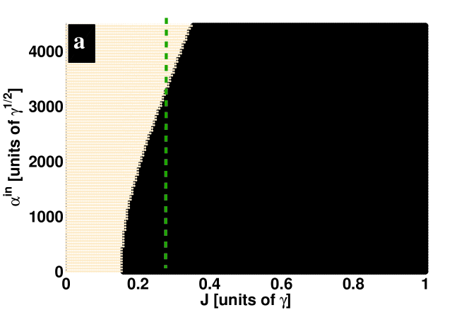
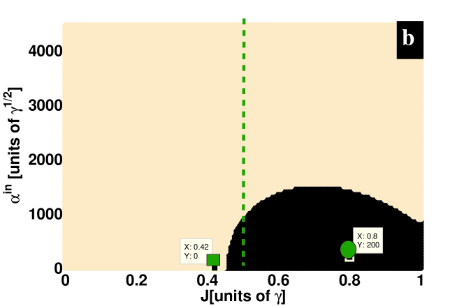
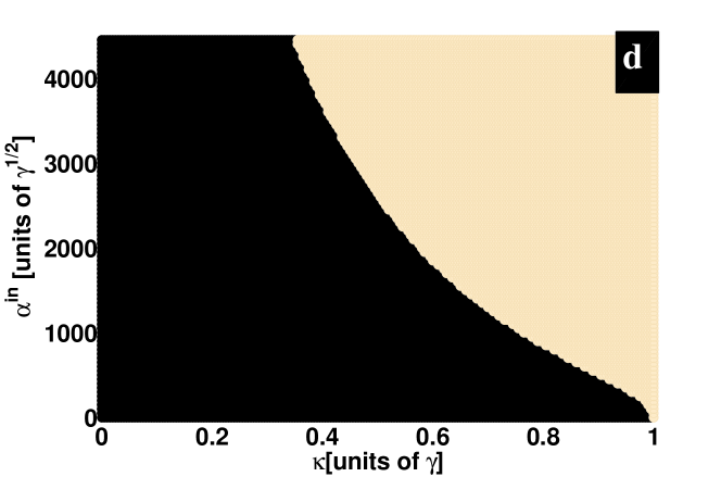
Figure 2: Basins of stability for the steady states. (a),(b). The evolution of stable (dark area) and unstable (light area) zones as the system gets closer to the balanced gain and loss limit. (a) $\kappa=0.1\gamma$; (b) $\kappa=0.8\gamma$. (c),(d) The evolution of stable (dark area) and unstable (light area) zones as the tunneling coupling $J$ increases. (c) $J=0.2\gamma$; (d) $J=\gamma$. These figures are obtained for $\chi=0$.

The linear stability of our system is mapped out through the basins of stability shown in Fig. 2. These figures are obtained in the absence of the PA ($\chi=0$). The steady states are stable for the range of parameters located in the blue space, while the red area corresponds to the parameters leading to unstable fixed points. It follows that the unstable area widens as the system moves towards the balanced gain and loss [compare Figs. 2(a) and 2(b)]. We also remark that the stability of the system is extended to large driving strength compared to the single lossy cavity (compare black and other colors in Fig. 3a). From Fig. 2c and Fig. 2d, it appears that the stability of the system improves as the tunneling coupling $J$ increases. Still, the stable steady states are shifted towards relatively large driving strength. In light of this discussion on the stability in active-passive COM, we conclude that (i) the steady-state solutions are stable for the imbalanced gain and loss system (weak $\kappa$), and (ii) stability can be improved by increasing the tunneling rate $J$, by pushing the system in the unbroken-$\mathcal{PT}$-symmetry regime. Another observed feature is the stability of the fixed points related to the EP. Such points are located along the green dashed lines in Figs. 2(a) and 2(b), for $\kappa=0.1\gamma$ (or $J=0.275\gamma$) and $\kappa=0.8\gamma$ (or $J=0.45\gamma$) respectively. It can be seen that the solutions along the EP lose their stability as the system approaches the gain-loss balance. Indeed, we have observed that at the exact gain-loss balance, the EP is completely in the unstable zone (no represented). From this analysis and in light of Figs. 2(a) and 2(b), it is shown that the stable steady states in active-passive COM are mostly located in the unbroken-$\mathcal{PT}$-symmetry regime.

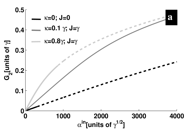
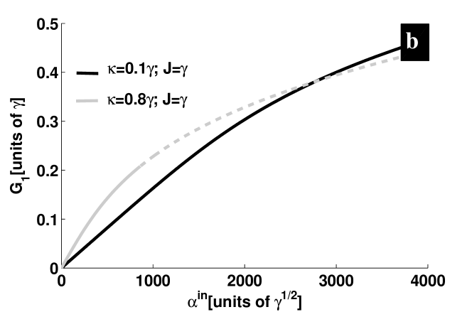
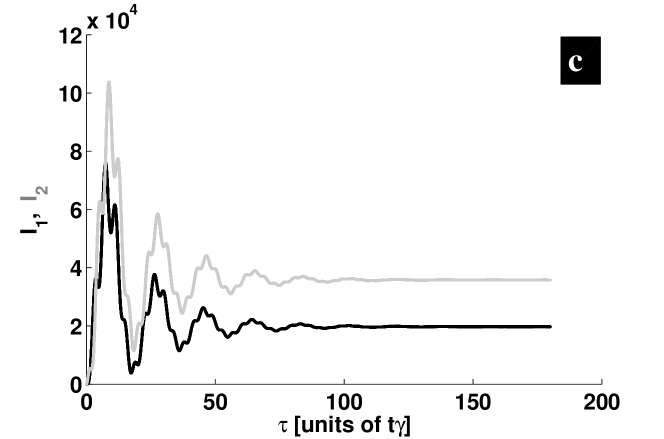
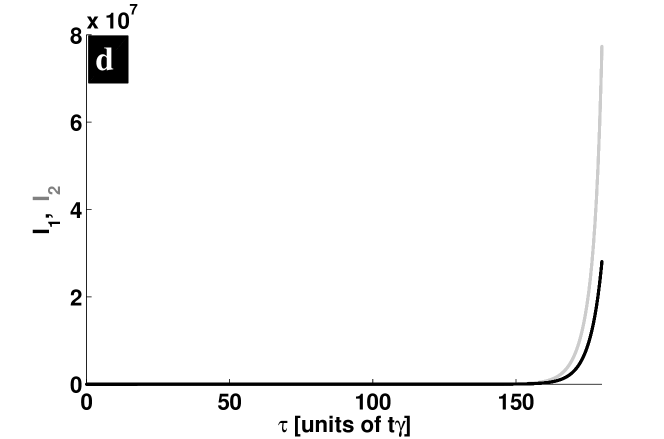
Figure 3: Evolution of steady states accordingly to the stability shown in Fig. 2. (a),(b) $G_{i}=g|\alpha_{i,s}|,\,i=1,2$, are the couplings strength. Solid lines are stable while dashed line are unstable. (c),(d) Time evolution of steady states having stable and unstable dynamics respectively, with $I_{i}=|\alpha^{*}_{i}\alpha_{i}|,\,i=1,2$. The parameters are (c) $\alpha^{in}=10^{2}\sqrt{\gamma}$, $J=0.8\gamma$ and $\kappa=0.8\gamma$, and (d) $\alpha^{in}=10^{-5}\sqrt{\gamma}$, $J=0.42\gamma$ and $\kappa=0.8\gamma$. For all of these figures, $\chi=0$ and the index $i=1$ is related to the lossy cavity whereas the index $i=2$ stands for the gain cavity.

As the gain cavity is coupled to the mechanical resonator through the loss cavity, one can define the resulting (distant) coupling as $G_{1}=g|\alpha_{1,s}|$. This suggests the idea of investigating distant entanglement between the gain cavity and the mechanical resonator. Figures 3(a) and 3(b) show the couplings $G_{2}$ and $G_{1}$ versus the driving pump $\alpha^{in}$, respectively. Full lines are stable while dashed lines are unstable, in accordance with the stability shown in Fig. 2. For $\chi=0$, Figs. 3(a) and 3(b) show the enhancement of the couplings $G_{2}$ and $G_{1}$ as well as the improvement of the system’s stability (gray colors) compared to the conventional COM case [black color in Fig. 3(a)]. As a result, the steady states are more stable in the systems having gain and loss, and this paves a way to use such systems to enhance the quantum effect as for entanglement here. As the system moves from imbalanced gain and loss to the balanced case, the magnitude of the couplings $G_{1,2}$ slightly increases while the stability is impaired [see Figs. 3(a) and 3(b)]. We have remarked that $\chi$ slightly enhances the couplings $G_{1,2}$ (not represented), and this effect will be highlighted through the entanglement later on. It is shown that, (i) stability is improved in the unbroken-$\mathcal{PT}$-symmetry regime and (ii) the couplings $G_{1,2}$ are enhanced when approaching gain and loss balance. Based on this discussion, we have determined which regime to study distant entanglement. But first, we have performed the validity of the above stability analysis through a numerical simulation of Eq. (2). Figure 3(c) corresponds to the stable steady state solution indicated by the green dot in Fig. 2(b). Figure 3(d) shows the dynamical state of the unstable fixed point localized in the vicinity of the green square in Fig. 2(b). We can see that the solution is attracted to a fixed point in Fig. 3(c) while it grows exponentially in Fig. 3(d). This exponential growth is reminiscent of instabilities, and the long-time study of such behavior yields a limit cycle or chaotic dynamics. This numerical investigation ensures the veracity of our stability analysis.

IV Entanglement generation

To measure the CV entanglement between the gain cavity and the mechanical modes, we use the standard ensemble method, which consists of computing the logarithmic negativity through the quantum fluctuations of the system’s quadratures [7] ; [8] . From the set of fluctuation equations given in Eq. (5), we can define the vector of quadratures $u(t)=\left(\delta x(t),\delta p(t),\delta I_{1}(t),\delta\varphi_{1}(t),\delta I_{2}(t),\delta\varphi_{2}(t)\right)^{T}$ and the vectors of noises $n(t)=\left(\delta I_{x}^{in}(t),\delta I_{p}^{in}(t),\delta I_{1}^{in}(t),\delta\varphi_{1}^{in}(t),\delta I_{2}^{in}(t),\delta\varphi_{2}^{in}(t)\right)^{T}$. Thus, the system’s quadratures can be written in the compact form

$$\dot{u}(t)=Au(t)+n(t),$$ (8)

with the correlation matrix

$$A=\begin{bmatrix}-\frac{\gamma_{m}}{2}&\omega_{m}&0&0&0&0\\ -\omega_{m}&-\frac{\gamma_{m}}{2}&0&0&2G_{2}&0\\ 0&0&\frac{\kappa}{2}&-\Delta&0&J\\ 0&0&\Delta&\frac{\kappa}{2}&-J&0\\ 0&0&0&J&(2\chi\cos\theta-\frac{\gamma}{2})&(2\chi\sin\theta-\tilde{\Delta})\\ 2G_{2}&0&-J&0&(2\chi\sin\theta+\Delta)&-(2\chi\cos\theta+\frac{\gamma}{2})\end{bmatrix}.$$ (9)

The above quadrature operators are defined as, $\delta X=(\delta\mathcal{O}^{\dagger}+\delta\mathcal{O})/\sqrt{2}$ and $\delta Y=i(\delta\mathcal{O}^{\dagger}-\delta\mathcal{O})/\sqrt{2}$, with $X\equiv(x,I_{i=1,2})$ and $Y\equiv(p,\varphi_{i=1,2})$. Similarly, the noises quadratures are given by $\delta X^{in}=(\delta\mathcal{O}^{in{\dagger}}+\delta\mathcal{O}^{in})/\sqrt{2}$ and $\delta Y^{in}=i(\delta\mathcal{O}^{in{\dagger}}-\delta\mathcal{O}^{in})/\sqrt{2}$, with $X^{in}\equiv(I_{x}^{in},I_{i=1,2}^{in})$ and $Y^{in}\equiv(I_{p}^{in},\varphi_{i=1,2}^{in})$. The noise operators $\beta^{in},\alpha_{1}^{in}$, and $\alpha_{2}^{in}$ have zero mean, and are characterized by the following auto correlation functions [9] ; [20] :

$$\begin{cases}\langle\delta s^{in}(t)\delta s^{in{\dagger}}(t^{\prime})\rangle=(n_{\sigma}+1)\delta(t-t^{\prime}),\\ \langle\delta s^{in{\dagger}}(t)\delta s^{in}(t^{\prime})\rangle=n_{\sigma}\delta(t-t^{\prime}),\end{cases}$$ (10)

with $\delta s^{in}\equiv(\beta^{in},\alpha_{1}^{in},\alpha_{2}^{in}$) and $n_{\sigma}\equiv(n_{th},n_{a})$, where $n_{th}=\left[\exp\left(\frac{\hbar\omega_{m}}{k_{B}T}\right)-1\right]^{-1}$ and $n_{a}=\langle\alpha_{1,2}^{in{\dagger}}\alpha_{1,2}^{in}\rangle$.

When the system is stable, one gets the following equation for the steady-state covariance matrix (CM) [7] ; [8] :

$$AV+VA^{T}=-D.$$ (11)

Here, the CM is a $6\times 6$ matrix and the elements of the diffusion matrix $D$ are defined by

$$\delta(t-t^{\prime})D_{i,j}=\frac{1}{2}\langle n_{i}(t)n_{j}^{\dagger}(t^{\prime})+n_{j}^{{\dagger}}(t)n_{i}(t^{\prime})\rangle.$$ (12)

Using Eq. (10), one obtains

$$D=diag\left[\frac{\gamma_{m}}{2}(2n_{th}+1),\frac{\gamma_{m}}{2}(2n_{th}+1),\frac{\kappa}{2}(2n_{a}+1),\frac{\kappa}{2}(2n_{a}+1),\frac{\gamma}{2}(2n_{a}+1),\frac{\gamma}{2}(2n_{a}+1)\right].$$ (13)

In order to evaluate the entanglement between two subsystems (bipartite entanglement), the CM should be rewritten as [8]

$$V=\begin{pmatrix}V_{\beta}&V_{\beta,\alpha_{1}}&V_{\beta,\alpha_{2}}\\ V_{\beta,\alpha_{1}}^{T}&V_{\alpha_{1}}&V_{\alpha_{2},\alpha_{1}}\\ V_{\beta,\alpha_{2}}^{T}&V_{\alpha_{2},\alpha_{1}}&V_{\alpha_{2}}\end{pmatrix}$$ (14)

where each block represents a $2\times 2$ matrix. The blocks on the diagonal indicate the variance within each subsystem, while the off-diagonal blocks indicate the covariance across different subsystems, i.e., the correlations between two components that describe their entanglement property. To compute the pairwise entanglement, we reduce the covariance matrix $V$ to a $4\times 4$ submatrix $V_{S}$,

$$V_{S}=\begin{pmatrix}V_{k\equiv(\beta,\alpha_{1},\alpha_{2})}&V_{k,\ell}\\ V_{k,\ell}^{T}&V_{\ell\equiv(\beta,\alpha_{1},\alpha_{2})}\end{pmatrix},$$ (15)

depending on which subsystems we are interested in.

The logarithmic negativity is then defined as [8]

$$E_{N}=\max[0,-\ln 2\eta],$$ (16)

where

$$\eta=\sqrt{\frac{\sum-\sqrt{\sum^{2}-4\det V_{S}}}{2}},$$ (17)

is the lowest symplectic eigenvalue of the partial transpose of the submatrix $V_{S}$ with

$$\sum=\det V_{k}+\det V_{\ell}-2\det V_{k,\ell}.$$ (18)

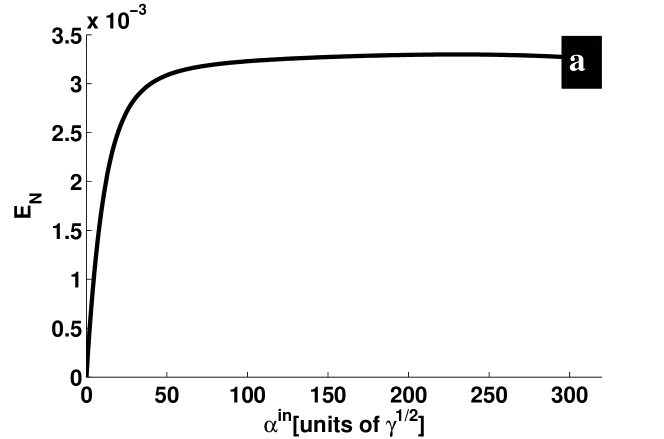
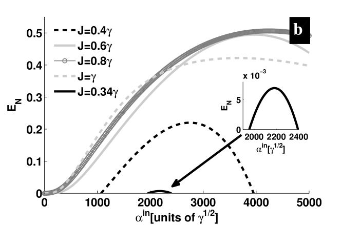
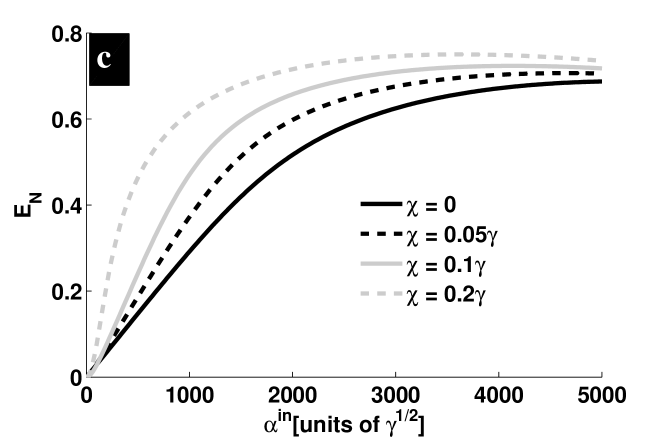
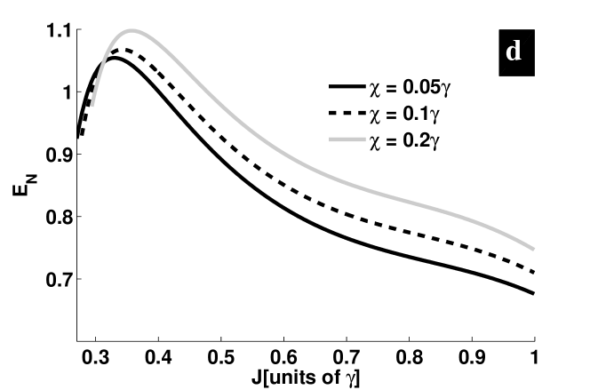
Figure 4: (a) Logarithmic negativity $E_{N}$ vs $\alpha^{in}$ in the conventional COM. (b),(c) The entanglement $E_{N}$ vs $\alpha^{in}$ between the gain cavity and the mechanical modes. (b) $\chi=0$, $\kappa=0.1\gamma$ and different values of $J$. (c) $E_{N}$ vs $\alpha^{in}$, for $\kappa=10^{-5}\gamma$, $J=\gamma$ and different values of $\chi$. (d) $E_{N}$ vs $J$ for $\alpha^{in}=3\times 10^{3}\sqrt{\gamma}$, $\kappa=10^{-5}\gamma$ and different values of $\chi$. These curves are plotted in the absence of noises ($n_{th}=n_{a}=0$).

One can now characterize the entanglement through Eq. (16). Figure 4(a) shows $E_{N}$ versus the driving $\alpha^{in}$ in the single lossy cavity. One remarks that, the mechanical resonator mode $\beta$ and the optical cavity mode $\alpha_{2}$ are entangled ($E_{N}>0$). We note that this entanglement is weak and is limited by stability conditions that put constraints on the magnitude of the couplings $G_{1,2}$ [see black curve in Fig. 3(a)]. This result agrees well with what is predicted in single lossy cavity optomechanics [27] -[29] . In order to enhance entanglement, we consider the gain and loss COM system since it improves the couplings [see gray curves in Figs. 3(a) and 3(b)]. As our interest is on distant entanglement, we expect it to be enhanced in light of Fig. 3(b). Figure 4(b) shows entanglement between the gain cavity and the mechanical modes versus $\alpha^{in}$. We remark the improvement of the entanglement compared to what is generated in the conventional COM [see Fig. 4(a]). This enhancement happens in the unbroken-$\mathcal{PT}$-symmetry regime. Indeed, the EP corresponds to $J=0.275\gamma$ and there is no entanglement there (not represented). Indeed, the entanglement starts at $J=0.34\gamma$, which is beyond the EP [see the black curve in Fig. 4(b)]. One also remarks that, moving from the broken to the unbroken-$\mathcal{PT}$-symmetry regimes, the entanglement is enhanced even for weak driving strength [compare black curves to the others curves in Fig. 4(b)].

Similar distant entanglement has been investigated in [41] ; [42] by coupling two lossy cavities, both supporting a mechanical resonator. Because of the absence of $\mathcal{PT}$-symmetry, the generated entanglement as relatively weak compared to what is obtained here. Indeed, adiabatic approximation was used in [41] and both cavities were driven by blue-detuned lasers. The resulting amount of entanglement was weak compared to what is generated in [42] . However, by driving the cavities by blue- and red-detuned lasers, respectively, it is shown that, the amount of generated entanglement increases [42] . In this work, we point out that $\mathcal{PT}$-symmetry has boosted the generation of entanglement in our system.

The effect of the PA on the entanglement is shown in Fig. 4(c). As the gain $\chi$ of the PA increases, the entanglement enhances, but mostly for relatively weak driving strength $\alpha^{in}$. With the help of the stability studied in Sec. III, the entanglement can be further enhanced as shown in Fig. 4(d).

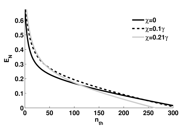
Figure 5: Logarithmic negativity $E_{N}$ versus thermal noise $n_{th}$, for $\alpha^{in}=3\times 10^{3}\sqrt{\gamma}$, $\kappa=10^{-5}\gamma$, $J=0.8\gamma$, and different values of $\chi$.

It is also important to address the effect of noises on the studied entanglement. Such concern addresses the robustness of this kind of entanglement against decoherence. This is investigated in Fig. 5, where entanglement is plotted versus thermal noise for $n_{a}=10^{-3}$. One remarks that the optical mode inside the gain cavity and the mechanical mode are still entangled for thermal noise up to $n_{th}=300$. However, the weakness of the entanglement against thermal noise can be pointed out in the presence of the PA (compare gray and black curves in Fig. 5). It is shown that the entanglement is enhanced in gain and loss COM compared to the conventional case. Furthermore, this entanglement is improved in the presence of the PA as already stated in Refs. [14], and [14a], . The robustness of this entanglement against decoherence is highlighted.

It is noteworthy that the combined effects of PA and the gain cavity lead to instabilities. In order to avoid these instabilities and to investigate the effect of $\chi$, we considered the far imbalanced cavities case by choosing a small value of $\kappa$ [see Figs. 4 (c), (d) and 5].

In order to show enhancement of entanglement in the $\mathcal{PT}$-symmetry system compared to what is generated in a lossy coupled COM, we address a comparative study with lossy coupled COM [41] ; [42] . By choosing a negative value of $\kappa$ ($\kappa<0$), our coupled COM presented in (Fig. 1) becomes a lossy coupled COM [34] ; [41] ; [42] . The amount of distant entanglement is captured by the logarithmic negativity as described before. We first compare the couplings resulting in both configurations, and then conclude regarding the induced entanglement. Figures. 6(a) and 6(b) compare the effective coupling $G_{1}$ for $|\kappa|=0.1\gamma$ and $|\kappa|=0.8\gamma$, respectively. The full lines are stable while the dashed ones are unstable. In both cases, the coupling strength is improved in the gain and loss COM and this is an indication that entanglement will be enhanced accordingly as well. Remarkably, the couplings get closer as $|\kappa|$ decreases. Indeed, the couplings are closer for $|\kappa|=0.1\gamma$ [Fig. 6(a)] than for $|\kappa|=0.8\gamma$ [Fig. 6(b)]. Furthermore, we have checked that for weak value of $\kappa$ ($|\kappa|\approx 5\times 10^{-2}\gamma$), there is no difference (at least on the coupling strength) between the $\mathcal{PT}$-symmetry COM case and the lossy coupled cavities case. Figures 6(c) and 6(d) show distant entanglement generated in both configurations for $|\kappa|=0.1\gamma$ with $J=\gamma$ and $J=0.8\gamma$ respectively. The entanglement captured in Fig. 6(c) corresponds to the coupling shown in Fig. 6(a). As expected, the generated entanglement in the $\mathcal{PT}$-symmetry configuration is slightly enhanced compared to what is obtained in the lossy coupled COM case [see Fig. 6(c)]. Let us keep in mind that, weak coupling rate $J$ can be related to a large distance between cavities while strong coupling rate $J$ means a tiny separation between them. In this sense, one deduces from Fig. 4(d) that, as the separation between the cavities increases, the distant entanglement decreases. As $J=0.8\gamma$ in Fig. 6(d), we deduce that the $\mathcal{PT}$-symmetry COM is the best configuration to enhance distant entanglement. Indeed, by decreasing the coupling rate $J$ (increasing the separation) one gets a net enhancement of distant entanglement in the $\mathcal{PT}$-symmetry case compared to what is generated in the lossy coupled COM (Fig. 6d). Thus, $\mathcal{PT}$-symmetry COM is a good candidate to enhance distant entanglement.

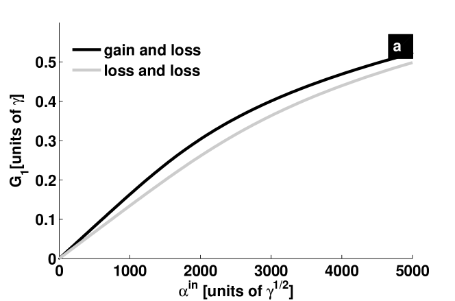
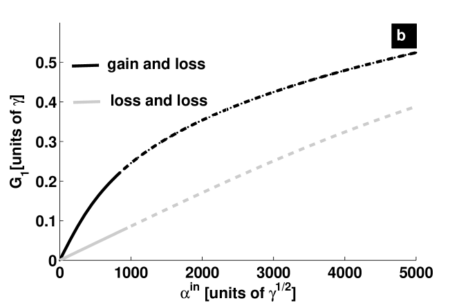
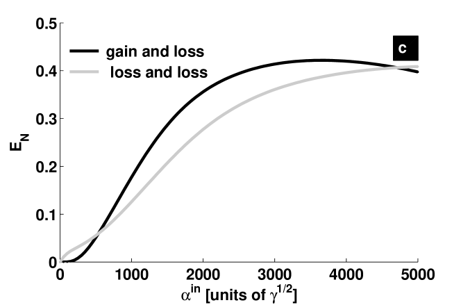
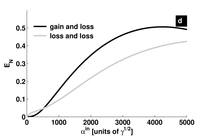
Figure 6: (a),(b) The effective optomechanical coupling $G_{1}$ versus the driving $\alpha^{in}$ for $J=\gamma$, with (a)$\kappa=0.1\gamma$ and (b) $\kappa=0.8\gamma$. (c),(d) The distant entanglement vs the driving $\alpha^{in}$ for $\kappa=0.1\gamma$ with (c) $J=\gamma$ and (d) $J=0.8\gamma$. Black lines are for the gain and loss coupled cavities while the blue lines are for the loss and loss coupled cavities. Full lines are stable and the dashed lines are unstable.

V Conclusion

We have studied a system of coupled active and passive resonators with the focus on steady states stability analysis and the possible generation of distant CV entanglement. We have shown through linear stability analysis that, the steady-state solutions are generally unstable in the broken-$\mathcal{PT}$-symmetry regime and are more stable in the unbroken-$\mathcal{PT}$-symmetry phase. The general statement follows that, the system is more stable (unstable) for large (small) tunneling coupling rate $J$. Conversely, the system is stable (unstable) for small (large) gain-loss parameter. We found that the stable solutions correspond to relatively large driving strength, compared to the single loss cavity case. Consequently, this increases the optomechanical coupling between the mechanical mode and the optical field inside the gain cavity. It results in an enhancement of steady-state CV entanglement between these modes. It also appears from a comparative study with lossy coupled COM that, for weak values of $\kappa$, there is no difference between the two cases, regarding the coupling and the entanglement; and for large $\kappa$, there is a net enhancement of both coupling and entanglement in the gain-loss case compared to what is obtained in the loss-loss cavities case. For more entanglement generation, this work suggests exploitation the presence of a squeezing element inside the active-passive COM. Such nonclassical states can represent an ideal playground for investigating and comparing decoherence theories and modifications of quantum theory at the macroscopic level.

- (1) M. Aspelmeyer, T. J. Kippenberg, and F. Marquardt, Rev. Mod. Phys. 86, 1391 (2014).
- (2) A. D. O’Connell, M. Hofheinz, M. Ansmann, R. C. Bialczak, M. Lenander, E. Lucero, M. Neeley, D. Sank, H. Wang, M. Weides, J. Wenner, J. M. Martinis, and A. N. Cleland, Nature (London) 464, 697 (2010).
- (3) J. D. Teufel, T. Donner, D. Li, J. W. Harlow, M. S. Allman, K. Cicak, A. J. Sirois, J. D. Whittaker, K. W. Lehnert, and R. W. Simmonds, Nature (London) 475, 359 (2011); J. Chan, T. P. M. Alegre, A. H. Safavi-Naeini, J. T. Hill, A. Krause, S. Gröblacher, M. Aspelmeyer, and O. Painter, Nature (London) 478, 89 (2011).
- (4) A. Jöckel, A. Faber, T. Kampschulte, M. Korppi, M. T. Rakher, and P. Treutlein, Nat. Nanotechnol. 10, 55 (2015).
- (5) E. E. Wollman, C. U. Lei, A. J. Weinstein, J. Suh, A. Kronwald, F. Marquardt, A. A. Clerk, and K. C. Schwab, Science 349, 952 (2015).
- (6) F. Lecocq, J. B. Clark, R. W. Simmonds, J. Aumentado, and J. D. Teufel, Phys. Rev. X 5, 041037 (2015).
- (7) D. Vitali, S. Gigan, A. Ferreira, H. R. Böhm, P. Tombesi, A. Guerreiro, V. Vedral, A. Zeilinger, and M. Aspelmeyer, Phys. Rev. Lett. 98, 030405 (2007).
- (8) P. Djorwe, S. G. Nana Engo, and P. Woafo, Phys. Rev. A 90, 024303 (2014).
- (9) R.-X. Chen, L.-T. Shen, Z.-B. Yang, H.-Z. Wu, and S.-B. Zheng, Phys. Rev. A 89, 023843 (2014).
- (10) T. Huan, R. Zhou, and H. Ian, Phys. Rev. A 92, 022301 (2015).
- (11) G. Wang, L. Huang, Y.-C. Lai, and C. Grebogi, Phys. Rev.Lett. 112, 110406 (2014).
- (12) M. Tsang, Phys. Rev. A 81, 063837 (2010).
- (13) M. Paternostro, D. Vitali, S. Gigan, M.S. Kim, C. Brukner, J. Eisert, and M. Aspelmeyer, Phys. Rev. Lett. 99, 250401 (2007).
- (14) A Mari and J. Eisert, Phys. Rev. Lett. 103, 213603 (2009).
- (15) M. Abdi and M. J. Hartmann, New J. Phys. 17 013056 (2015); P. Degenfeld-Schonburg, M. Abdi, M. J. Hartmann, and Carlos Navarrete-Benlloch, Phys. Rev. A 93, 023819 (2016).
- (16) M. Ludwig, K. Hammerer, and F. Marquardt, Phys. Rev. A 82, 012333 (2010).
- (17) C. A. Muschik, E. S. Polzik, and J. I. Cirac, Phys. Rev. A 83, 052312 (2011).
- (18) H. Krauter, C. A. Muschik, K. Jensen, W. Wasilewski, J. M. Petersen, J. I. Cirac, and E. S. Polzik, Phys.Rev.Lett. 107, 080503 (2011).
- (19) K. Borkje, A. Nunnenkamp, and S. M. Girvin, Phys. Rev.Lett. 107, 123601 (2011).
- (20) H. T. Tan and G. X. Li, Phys. Rev. A 84, 024301 (2011).
- (21) L. Tian, Phys. Rev.Lett. 110, 233602 (2013).
- (22) J. Li, I. M. Haghighi, N. Malossi, S. Zippilli, and D. Vitali, New J. Phys. 17, 103037 (2015).
- (23) M. Asjad, S. Zippilli, and D. Vitali, Phys. Rev. A 93, 062307 (2016).
- (24) A. Mari and J. Eisert, Phys. Rev. Lett. 108, 120602 (2012) and references therein.
- (25) M. J. Hartmann and M. B. Plenio, Phys. Rev. Lett. 101, 200503 (2008); Phys. Rev. A 89, 014302 (2014); Phys. Rev. A 91, 013807 (2015); Phys. Rev. Lett. 114, 173602 (2015) or New J. Phys. 18 (2016) 063022.
- (26) J.-Q. Liao and L. Tian, Phys. Rev.Lett. 116, 163602 (2016).
- (27) S. Forstner, J. Knittel, E. Sheridan, J. D. Swaim, H. R. Dunlop, and W. P. Bowen, Photonic Sensors 2, 259 (2012).
- (28) S. Rips, and M.J. Hartmann, Phys. Rev. Lett. 110, 120503 (2013).
- (29) K. Stannigel, P. Komar, S. J. M. Habraken, S. D. Bennett, M. D. Lukin, P. Zoller, and P. Rabl, Phys. Rev. Lett. 109, 013603 (2012).
- (30) S. L. Braunstein, and P. van Loock, Rev. Mod. Phys. 77, 513 (2005).
- (31) C. A. Muschik, K. Hammerer, E. S. Polzik, and I. J. Cirac, Phys. Rev. Lett. 111, 020501 (2013).
- (32) S. Barzanjeh, S. Pirandola, and C. Weedbrook, Phys. Rev. A 88, 042331 (2013).
- (33) J. Stolze and D. Suter, Quantum Computing: A Short Course from Theory to Experiment (Wiley-VCH, Dortmund, 2004).
- (34) D. Stucki, M. Legré, F. Buntschu, B. Clausen, N. Felber, N. Gisin, L. Henzen, P. Junod, G. Litzistorf, P. Monbaron, L. Monat, J.-B. Page, D. Perroud, G. Ribordy, A. Rochas, S. Robyr, J Tavares, R. Thew, P. Trinkler, S. Ventura, R. Voirol, N. Walenta1, and H Zbinden, New J. Phys. 13, 123001 (2011).
- (35) H. Jing, S. K. , H. L, F. Nori, arXiv:1609.01845.
- (36) H. Jing, S. K. Ozdemir, X.-Y. Lu, J. Zhang, L. Yang, and F. Nori, Phys. Rev. Lett.113, 053604 (2014).
- (37) X.-Y. Lu, H. Jing, J.-Y. Ma, and Y. Wu, Phys. Rev. Lett. 114, 253601 (2015).
- (38) D.W. Schönleber, A. Eisfeld, and R. El-Ganainy, New J.Phys. 18, 045014 (2016).
- (39) H. Xu, D. Mason, L. Jiang, and J.G.E. Harris, Nature (London) 537, 80 (2016).
- (40) X.-W. Xu, Y.-X. Liu, C.-P. Sun, and Y. Li, Phys.Rev. A 92, 013852 (2015).
- (41) B. Peng, Ş. K. Özdemir, F. Lei, F. Monifi, M. Gianfreda, G. L. Long, S. Fan, F. Nori, C. M. Bender, and L. Yang, Nat. Phys. 10, 394 (2014); B. Peng, Ş. K. Özdemir, S. Rotter, H. Yilmaz, M. Liertzer, F. Monifi, C. M. Bender, F. Nori, and L. Yang, Science 346, 328 (2014).
- (42) L. Chang, X. Jiang, S. Hua, C. Yang, J. Wen, L. Jiang, G. Li, G. Wang, and M. Xiao, Nat. Photon. 8, 524 (2014).
- (43) J. Fan and L. Zhu, Opt. Express 20, 20790 (2012).
- (44) C. M. Bender, M. Gianfreda, S. K. Ozdemir, B. Peng, and L. Yang, Phys. Rev. A 88, 062111 (2013).
- (45) C. Joshi, J. Larson, M. Jonson, E. Andersson, and P. Ohberg, Phys. Rev. A 85, 033805 (2012).
- (46) Uzma Akram, William Munro, Kae Nemoto, and G. J. Milburn, Phys. Rev. A 86, 042306 (2012).
- (47) S. Strogatz, Nonlinear Dynamics and Chaos: With Applications to Physics, Biology, Chemistry, and Engineering (Studies in Nonlinearity) (Boulder, CO: Westview Press, 2014).