The Hi-GAL compact source catalogue.
I. The physical properties of the clumps in the inner Galaxy ($-71.0^{\circ}<\ell<67.0^{\circ}$)

Abstract

Hi-GAL is a large-scale survey of the Galactic plane, performed with Herschel in five infrared continuum bands between 70 and 500 $\mu$m. We present a band-merged catalogue of spatially matched sources and their properties derived from fits to the spectral energy distributions (SEDs) and heliocentric distances, based on the photometric catalogs presented in Molinari et al. (2016a), covering the portion of Galactic plane $-71.0^{\circ}<\ell<67.0^{\circ}$. The band-merged catalogue contains 100922 sources with a regular SED, 24584 of which show a 70 $\mu$m counterpart and are thus considered proto-stellar, while the remainder are considered starless. Thanks to this huge number of sources, we are able to carry out a preliminary analysis of early stages of star formation, identifying the conditions that characterise different evolutionary phases on a statistically significant basis. We calculate surface densities to investigate the gravitational stability of clumps and their potential to form massive stars. We also explore evolutionary status metrics such as the dust temperature, luminosity and bolometric temperature, finding that these are higher in proto-stellar sources compared to pre-stellar ones. The surface density of sources follows an increasing trend as they evolve from pre-stellar to proto-stellar, but then it is found to decrease again in the majority of the most evolved clumps. Finally, we study the physical parameters of sources with respect to Galactic longitude and the association with spiral arms, finding only minor or no differences between the average evolutionary status of sources in the fourth and first Galactic quadrants, or between “on-arm” and “inter-arm” positions.

1 Introduction

The formation of stars remains one of the most important unsolved problems in modern astrophysics. In particular, it is not clear how massive stars ($M>8$ M_⊙) form, despite their importance in the evolution of the Galactic ecosystem (e.g., Ferrière, 2001; Bally & Zinnecker, 2005). The formation of high-mass stars is not as well-understood as that of low-mass stars, mainly because of a lack of observational facts upon which models can be built. High-mass stars are intrinsically difficult to observe because of their low number in the Galaxy, their large distance from the Sun and their rapid evolution. Numerous observational surveys have been undertaken in recent years in different wavebands to obtain a better statistics on massive pre- and proto-stellar objects. (Jackson et al., 2006; Stil et al., 2006; Lawrence et al., 2007; Churchwell et al., 2009; Carey et al., 2009; Schuller et al., 2009; Rosolowsky et al., 2010; Hoare et al., 2012; Urquhart et al., 2014a; Moore et al., 2015). Among these, Hi-GAL is the only complete far-infrared (FIR) survey of the Galactic plane.

Hi-GAL (Herschel InfraRed Galactic Plane Survey, Molinari et al., 2010a) is an Open Time Key Project that was granted about 1000 hours of observing time using the Herschel Space Observatory (Pilbratt et al., 2010). It delivers a complete and homogeneous survey of the Galactic plane in five continuum FIR bands between 70 and 500 $\mu$m. This wavelength coverage allows us to trace the peak of emission of most of the cold ($T<20$ K) dust in the Milky Way at high resolution for the first time, material that is expected to trace the early stages of the formation of stars across the mass spectrum. Hi-GAL data were taken using in parallel two of the three instruments aboard Herschel, PACS (70 and 160 $\mu$m bands, Poglitsch et al., 2010) and SPIRE (250, 350 and 500 $\mu$m bands, Griffin et al., 2010).

The present paper is meant to complete the discussions presented in Molinari et al. (2016a) on the construction of the photometric catalogue for the portion of Galaxy in the range -71.0${}^{\circ}\lesssim\ell\lesssim$ 67.0^∘, $|b|<1.0^{\circ}$, an area corresponding to the first Hi-GAL proposal (subsequently extended to the whole Galactic plane). In particular here we explain how we went from the photometric catalogue to the physical one, introducing band-merging, searching for counterparts, assigning distances as well as constructing and fitting spectral energy distributions (SEDs). In the last part of the paper, in which the distribution of sources with respect to their position in the Galactic plane is analysed in detail, we focus on two regions, i.e. 289.0${}^{\circ}<\ell<$ 340.0^∘ and 33.0${}^{\circ}<\ell<$ 67.0^∘. The innermost part of the Galactic plane, including the Galactic centre, where kinematic distance estimate is particularly problematic, will be discussed in a separated paper (Bally et al, in prep.), while the two longitude ranges containing the two tips of the Galactic bar ($340.0^{\circ}<\ell<350.0^{\circ}$ and $19.0^{\circ}<\ell<33.0^{\circ}$) have been presented in Veneziani et al. (2017).

1.1 Brief presentation of the surveyed regions

1.1.1 Fourth Galactic quadrant

In the longitude range investigated in more detail in this paper, three spiral arms are in view (see, in the following, Figure 1), according to a four-armed spiral model of the Milky Way (Urquhart et al., 2014a, and references therein). Moving towards the Galactic centre, for $289^{\circ}\lesssim\ell\lesssim 310^{\circ}$ the Carina-Sagittarius arm is observed, while at $\ell\sim 310^{\circ}$ the tangent point of the Scutum-Crux arm is encountered (García et al., 2014). The emission from this latter arm is expected to dominate up to the tangent point of the Norma arm at $\ell\sim 330^{\circ}$. Around this longitude, the main peak of the OB star formation distribution across the Galaxy is found (Bronfman et al., 2000). Finally, the tangent point of the subsequent arm, the so-called 3-kpc arm, is located at $\ell\sim 338^{\circ}$ (García et al., 2014), i.e. very close to the inner limit of the investigated zone.

Significant star formation activity is found in the surveyed region, as testified by the presence of 103 out of 481 star forming complexes in the list of Russeil (2003), and of 393 star forming regions out of 1735 in the Avedisova (2000) overall catalogue, 29 of which are H$\alpha$-emission regions of the RCW catalogue (Rodgers et al., 1960). Furthermore, 337 out of 1449 regions with embedded OB stars of the Bronfman et al. (1996); Bronfman et al. (2000) list are found in this region of the sky.

Hi-GAL observations of the fourth Galactic quadrant have been already used for studying InfraRed Dark Clouds (IRDCs, Egan et al., 1998) in the $300^{\circ}\lesssim\ell\lesssim 30^{\circ}$, $|b|\leq 1^{\circ}$ range (Wilcock et al., 2012a, b), highlighting the fundamental role of the Herschel FIR data for exploring the internal structure of these candidate sites for massive star formation. Furthermore, Veneziani et al. (2017) used the catalogue presented here to study the compact source population in the far tip of the long Galactic bar. These data will be exploited, if needed, in this article as well, for instance for comparison between the fields studied in this paper and inner regions of the Galaxy.

Finally, the nearby Coalsack nebula ($d=100-200$ pc, see references in Beuther et al., 2011) is also seen in the foreground of our field ($300^{\circ}\lesssim\ell\lesssim 307^{\circ}$, Wang et al., 2013). It is one of the most prominent dark clouds in the southern Milky Way but shows no evidence of recent star formation (e.g., Kato et al., 1999; Kainulainen et al., 2009).

1.1.2 First Galactic quadrant

In the first quadrant portion investigated in more detail in this paper ($33^{\circ}\lesssim\ell\lesssim 67^{\circ}$), two spiral arms are in view, namely the Carina-Sagittarius and the Perseus arms. The Carina-Sagittarius tangent point is found at $\ell\simeq 51^{\circ}$ (Vallée, 2008) near the W51 star forming region. From here to the endpoint of the region we are considering, only the Perseus arm is expected.

This area is smaller than that surveyed in the fourth quadrant and has a lower rate of star formation activity per unit area. Russeil (2003) finds 33 star-forming region in this area, and Avedisova (2000) finds just 97.

Hi-GAL studies of this portion of the Galactic plane mainly focused so far on one of the two Herschel Science Demonstration Phase fields, namely the one centered around $\ell=59^{\circ}$, regarding compact source physical properties obtained from earlier attempts of photometry of Hi-GAL maps (Elia et al., 2010; Veneziani et al., 2013; Beltrán et al., 2013; Olmi et al., 2013), structure of IRDCs (Peretto et al., 2010; Battersby et al., 2011), source and filament large-scale disposition (Billot et al., 2011; Molinari et al., 2010b; Bally et al., 2010), and diffuse emission morphology (Martin et al., 2010). As in the case of the fourth quadrant, the catalogue presented here has been already used by Veneziani et al. (2017) for studying the clump population at the near tip of the Galactic bar. Finally, a recent paper of Eden et al. (2015) focused on two lines of sight centred towards $\ell=30^{\circ}$ and $40^{\circ}$, studying arm/interarm differences in luminosity distribution of Hi-GAL sources.

1.2 Structure of the paper

The present paper is organised as follows: in Section 2, the data reduction, source detection and photometry strategy is briefly presented, referring to Molinari et al. (2010a) for further detail. In Section 3 SED building, filtering, complementing with ancillary photometry and distances are described. In Section 4 the use of a simple radiative model to derive the physical parameters of the Hi-GAL SEDs is illustrated, while the extraction of such properties from the photometry is summarised in Section 5. The statistics of the physical properties is discussed in Section 6, and the implications on the estimate of the evolutionary stage of sources are reported in Section 7. Finally, in Section 8, source properties are correlated with their Galactic positions: a comparison between sources in the IV and I Galactic quadrants is provided and, after positional matching of the sources and the locations of Galactic spiral arms, the behaviour of arm vs inter-arm sources is briefly discussed. Further details on how the catalogue is organised, and on possible biases affecting the listed quantities, are provided in the appendices at the end of the paper.

2 Data: map making and compact source extraction

The technical features of the Hi-GAL survey are presented in Molinari et al. (2010a), therefore here we limit ourselves to a summary of only the most relevant aspects. The Galactic plane was divided into $2^{\circ}\times 2^{\circ}$ sections, called “tiles” that were observed with Herschel at a scan speed of 60″s^-1 in two orthogonal directions. PACS and SPIRE were used in “Parallel mode” i.e. data were taken simultaneously with both instruments (and therefore at all five bands). Note that when used in Parallel mode, PACS and SPIRE observe a slightly different region of sky. A more complete coverage is nevertheless recovered when considering contiguous tiles; remaining areas of the sky covered only by either one of the two are not considered for science in this paper. Single maps of the Hi-GAL tiles were obtained from PACS/SPIRE detector timelines using a pipeline specifically developed for Hi-GAL and containing the ROMAGAL map making algorithm (Traficante et al. 2011) and the WGLS post-processing (Piazzo et al., 2012) for removing artefacts in the maps.

Astrometric consistency with Spitzer MIPSGAL 24 $\mu$m data (Carey et al., 2009, http://mipsgal.ipac.caltech.edu/) is obtained by applying a rigid shift to the entire mosaic. This is obtained as the mean shift measured on a number of bright and isolated sources common to Spitzer 24 $\mu$m and Hi-GAL PACS 70 $\mu$m data.

The further astrometric registration of SPIRE maps is then carried out by repeating the same procedure, but comparing counterparts of the same source at 160 and 250 $\mu$m.

Compact sources were detected and extracted using the algorithm CuTEx (Molinari et al. 2011) which is based on the study of the curvature of the images. This is done by calculating the second derivative at any pixel of the Hi-GAL images, efficiently damping all emission varying on intermediate to large spatial scales, and amplifying emission concentrated in small scales. This principle is particularly advantageous when extracting sources that appear within a bright and highly variable background emission. The final integrated fluxes are then estimated by CuTEx through a bi-dimensional Gaussian fit to the source profile. All details of the photometric catalogue are presented by Molinari et al. (2016a), who also report estimates of the completeness limits in flux in each band, measured by extracting a controlled 90% sample of sources artificially spread on a representative sample of real images. Such limits in the regions investigated in the present paper are discussed in Appendix C.2 for their implications on the estimate of source mass completeness limits as a function of the heliocentric distance.

The final version of the single-band catalogues of the portion of Hi-GAL data presented here contain 123210, 308509, 280685, 160972, and 85460 entries in the 70, 160, 250, 350 and 500 $\mu$m bands, respectively.

3 From photometry to physics

The present paper focuses on the study of compact cold objects extracted from Herschel data. Within this framework a final catalogue of objects for scientific studies has been obtained by merging the Hi-GAL single-band photometric catalogues and filtering the resulting five-band catalogue, applying specific constraints to the source SEDs. In the following sections the steps of these processes are explained in detail: band-merging, search for counterparts beyond the Herschel frequency coverage, assigning distances, SED filtering and fitting.

3.1 Band-merging and source selection

The first step for creating a multi-wavelength catalogue consists of assigning counterparts of a given source across Herschel bands. This operation based on iterating a positional matching (cf. Elia et al., 2010, 2013) between source lists obtained at two adjacent bands. In the present paper, however, instead of assuming a fixed matching radius as done in previous works, the matching region consisted of the ellipse describing the source at the longer of the two wavelengths. In other words, a source has a counterpart at shorter wavelength if the centroid of the latter falls within the ellipse fitted to the former. In this way it is possible that more than one counterparts falls into the longer-wavelength ellipse. In such multiplicity cases, the association is established only with the short-wavelength counterpart closest to the long-wavelength ellipse centroid. The remaining ones are reported as independent catalogue entries, and considered for further possible counterpart search at shorter wavelengths. At the end of the five band-merging, a catalogue is produced, in which each entry can contain from one to five detections in as many bands.

The subsequent step is to filter the obtained five-band catalogue in order to identify SEDs that are eligible for the modified black body (hereafter grey body) fit, hence to derive the physical properties of the objects. This selection is based on considerations of the regularity of the SEDs in the range 160-500 $\mu$m, since the 70 $\mu$m band generally is expected to depart from the grey body behaviour (e.g., Bontemps et al., 2010; Schneider et al., 2012).

First of all, as done in Elia et al. (2013), only sources belonging to the common PACS+SPIRE area and detected at least in three consecutive Herschel bands (i.e. the combinations 160-250-350 $\mu$m or 250-350-500 $\mu$m or, obviously, 160-250-350-500 $\mu$m) were selected.

Secondly, fluxes at 350 and 500 $\mu$m were scaled according to the ratio of deconvolved source linear sizes, taking as a reference the size at 250 $\mu$m (cf. Motte et al., 2010a; Nguyen Luong et al., 2011). This choice is supported by the fact that cold dust is expected to have significant emission around 250 $\mu$m; also, according to the adopted constraints to filter the SEDs, this is the shortest wavelength in common for all the selected SEDs. Finally, we searched for further irregularities in the SEDs such as dips in the middle, or peaks at 500 $\mu$m.

At the end of the filtering pipeline, we remain with 100922 sources. For each of these sources, we estimate physical parameters such as dust temperature, surface density and, when distance is available, linear size, mass, and luminosity, by fitting a single-temperature grey body to the SED. The details of this procedure are described in Section 4. Clearly, the determination of source physical quantities such as temperature and mass is more reliable when a better coverage of the SED is available. Based on the selection criteria listed above, sources in our catalogue can be confirmed, even considering the 70 $\mu$m flux, with detections at only three bands: this is the case for combinations 160-250-350 $\mu$m (with no detection at 70 $\mu$m) and 250-350-500 $\mu$m (that we call “SPIRE-only” sources), which we consider as genuine SEDs, although more affected by a less reliable fit (especially the SPIRE-only case, in which it might be difficult to constrain the SED peak, and consequently the temperature). For this reason, after the SED filtering procedure, we further split our SEDs in two sub-catalogues: “high reliability” (62438 sources) and “low reliability” (38484 sources). Notice that, according to the definitions that will be provided in Section 3.5, all the sources in the latter list belong to the class of “starless” compact sources.

In Table 1 the source number statistics for the band-merged catalogue is provided, divided in ranges of longitude (identified by the two intervals studied by Veneziani et al., 2017) and in evolutionary stages introduced in Section 3.5.

3.2 Caveats on SED building and selection

Building a five-band catalogue and selecting reliable sources for scientific analysis require a set of choices and assumptions which have been described in the previous sections. Here we collect and explicitly recall all of them to focus the reader’s attention on the limitations that must be kept in mind when using the Hi-GAL physical catalogue:

1. The concept of “compact source” used for this catalogue refers to unresolved or poorly resolved structures, whose size, therefore, does not exceed a few instrumental PSFs ($\lesssim 3$, Molinari et al., 2016a). Structures with larger angular sizes - such as bright diffuse interstellar medium (ISM), filaments, or bubbles - escape from this definition and are not considered in the present catalogue.

2. The appearance of the sky varies strongly throughout the wavelength range covered by Herschel. The lack of a detection in a given band may be ascribed to a detection error, or to the physical conditions of the source as, for instance, the case of a warm source seen by PACS but undetectable at the SPIRE wavelengths. In this respect, the present catalogue does not aim to describe all star formation activity within the survey area, but rather to provide a census of the coldest compact structures, corresponding to early evolutionary stages in which internal star formation activity has not yet been able to dissipate the dust envelope, or has not started at all. Detections at 70 $\mu$m only, or at 70/160 $\mu$m, or at 70/160/250 $\mu$m, are expected to have counterparts in the mid-infrared (MIR); such cases, corresponding to more evolved objects, surely deserve to be further studied, but this lies out of the aims of the present paper and is reserved for future works.

3. The band-merging procedure works fine in the ideal case of a source detected at all wavelengths as a bright and isolated peak. Possible multiplicities, however, can produce multiple branches in the counterpart association, so that, for instance, the flux at a given wavelength might result from the contributions of two or more counterparts detected separately at shorter wavelengths. This can also introduce inconsistent fluxes in the SEDs and produce irregularities such that several bright sources present in the Hi-GAL maps might be ruled out from the final catalogue according to the constraints described in Section 3.1.

4. Very bright sources might be ruled out by the filtering algorithm due to saturation occurring at one or more bands, which produces unrecoverable gaps in the SEDs.

5. The physical properties derived from Herschel SED analysis (see next sections) are global (e.g., mass, luminosity) or average (e.g. temperature) quantities for sources that, depending on their distance, can be characterised by a certain degree of internal but unresolved structure (see Section 6.1), as will be discussed in Appendix C.

3.3 Counterparts at non-Herschel wavelengths

For every entry in the band-merged filtered catalogue we searched for counterparts at 24 $\mu$m (MIPSGAL, Gutermuth & Heyer, 2015) as well as at 21 $\mu$m (MSX, Egan et al., 2003) and 22 $\mu$m (WISE, Wright et al., 2010). The fluxes of these counterparts, typically associated with a warm internal component of the clump, are not considered for subsequent grey-body fitting of the portion of the SED associated cold dust emission, but only for estimating the source bolometric luminosity.

In particular, we notice that the choice of sources in the catalogue of Gutermuth & Heyer (2015) is rather conservative, and only a small fraction has $F_{24}<0.005$ Jy. For this reason we performed an additional search of sources in the MIPSGAL maps, using APEX source extractor (Makovoz & Marleau, 2005) in order to recover those sources that, from a visual inspection of the maps, appear to be real although for some reason were not included in the original catalogue. Furthermore, as a cross-check, a similar procedure has been performed also with DAOFIND (Stetson, 1987), and only sources confirmed by this have been added to the photometry list of Gutermuth & Heyer (2015). Following this procedure, approximately 2000 additional SEDs have been complemented with a flux at 24 $\mu$m, mostly having fluxes in the 0.0001 Jy $<F_{24}<$ 0.001 Jy range. The risk of adding poorly reliable sources with low signal-to-noise ratio is mitigated by the fact that 24 $\mu$m counterparts of our Herschel sources are considered for scientific analysis only if they are confirmed by a detection at 70 $\mu$m (see Section 3.5 and Appendix B.

To assign counterparts to the Hi-GAL sources at 21, 22 and 24 $\mu$m, the ellipse representing the source at 250 $\mu$m was used as the matching region, and the flux of all counterparts at a given wavelength within this region was summed up into one value. Indeed, possible occurrences of multiplicity can induce a relevant contribution at MIR wavelengths in the calculation of bolometric luminosity of Hi-GAL sources.

On the long wavelength side of the SED we cross-matched our bandmerged and filtered catalogue with those of Csengeri et al. (2014) from the ATLASGAL survey (870 $\mu$m, Schuller et al., 2009) and of Ginsburg et al. (2013) from the BOLOCAM Galactic Plane Survey (BGPS, 1.1 mm Rosolowsky et al., 2010; Aguirre et al., 2011). The adopted searching radius was 19″ for the former and 33″ for the latter, corresponding to the full width at half maximum of the instruments at the observed wavelengths. Out of 10861 entries in the ATLASGAL catalogue, 10517 of them lie inside the PACS+SPIRE common science area considered in this paper, 6136 of which are found to be associated with a source of our catalogue through this 1:1 matching strategy. Similarly, 6020 out of 8594 entries of the BGPS catalogue lie in the common science area, 4618 of which turn out to be associated with an entry of our catalogue. Finally, access to ATLASGAL images allowed us to extract further counterparts, not reported in the list of Csengeri et al. (2014), by using CuTEx. In cases in which the deconvolved size of the ATLASGAL and/or BGPS counterpart is larger than the one measured at 250 $\mu$m, fluxes were re-scaled according to the procedure described in Section 3.1.

3.4 Distance determination

Assigning distances to sources is a crucial step in the process of giving physical significance to the information extracted from Hi-GAL data. While reliable distance estimates are available for a limited number of known objects, as for example H ii regions (e.g., Fish et al., 2003) or masers (e.g., Green & McClure-Griffiths, 2011), this information does not exist for the majority of Hi-GAL sources. Therefore we adopted the scheme presented in Russeil et al. (2011), based on the Galactic rotation model of Brand & Blitz (1993), to assign kinematic distances to a large proportion of sources: a ¹²CO (or ¹³CO) spectrum is extracted at the line of sight of every Hi-GAL source and the Velocity of the Local Standard of Rest $V_{\mathrm{LSR}}$ of the brightest spectral component is assigned to it, allowing the calculation of a kinematic distance. To determine the $V_{\mathrm{LSR}}$, the ¹³CO data from the Five College Radio Astronomy Observatory (FCRAO) Galactic Ring Survey (GRS, Jackson et al., 2006), and ¹²CO and ¹³CO data from the Exeter-FCRAO Survey (Brunt et al., in prep.; Mottram et al., in prep.) were used for the portion of Hi-GAL covering the first Galactic quadrant for $\ell<55^{\circ}$ and for $\ell>55^{\circ}$, respectively. The pixel size of those CO cubes is 22.5″, corresponding to Nyquist sampling of the FCRAO beam. NANTEN ¹²CO data (Onishi et al., 2005) were used to assign velocities to Hi-GAL sources in the fourth quadrant. The pixel size of these data is $4^{\prime}$ (against an angular resolution of $2^{\prime}.6$), so that more than one Hi-GAL source might fall onto the same CO line of sight, and the same distance is assigned to them. The spectral resolutions of the two data sets were 0.15 km s^-1 and 1.0 km s^-1, respectively.

Once the $V_{\mathrm{LSR}}$ is determined, the near/far distance ambiguity is solved by matching the source positions with a catalogue of sources with known distances (H ii regions, masers and others) or, alternatively, with features in extinction maps (in this case, the near distance is assigned). In cases for which none of the aforementioned data can be used, the ambiguity is always arbitrarily solved in favour of the far distance, and a “bad quality” flag is given to that assignment.

The additional use of extinction maps to solve for distance ambiguity (Russeil et al., 2011) (where applicable) can be a source of error, whose magnitude typically increases with increasing difference between the near and far heliocentric distance solutions. For the present paper, we rely on the use of extinction maps for practical reasons and also because, for most of the sources, no spectral line emission has yet been observed other than what can be extracted from the two CO surveys.

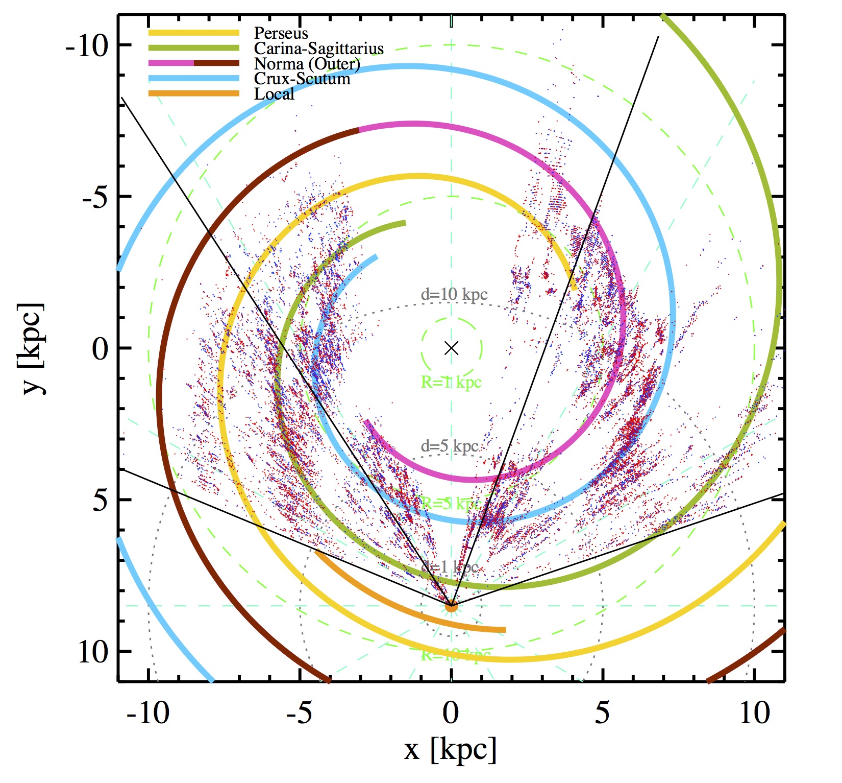
Figure 1: Plot of the position in the Galactic plane of the pre- (red dots) and proto-stellar (blue dots) Hi-GAL objects provided with a distance estimate. Unbound objects are not shown to reduce the crowding of the plot. For definitions of pre-stellar, proto-stellar and unbound objects, see Section 3.5. Two pairs of black solid lines delimit the longitude ranges analyzed in this paper. Further sources are found closer to the Galactic centre, most of which are analyzed in Veneziani et al. (2017) (see their Figure 1). In the inner zone devoid of points, distances were not estimated (see text), thus only distance-independent source properties were derived. The Galactic centre is indicated with a $\times$ symbol at coordinates $[x,y]=[0,0]$, the Sun with an orange dot at coordinates [0,8.5], at the bottom of the plot. Cyan dashed lines indicate Galactic longitude in steps of $30^{\circ}$. $R$ are Galactocentric distances (light green dashed circles), $d$ heliocentric ones (grey dotted circles), respectively, with the following steps: 1, 5 and 10 kpc. Spiral arms, from the four-arm Milky Way prescription of Hou et al. (2009), are plotted with different colours, with the arc-colour correspondence reported in the upper-left corner of the plot. In particular, the Norma arm is represented using two colours: magenta for the inner part of the arm, and brown for the portion of it generally designated as Outer arm, which starting point is established by comparison with Momany et al. (2006). Finally the Local arm, not included in the model of Hou et al. (2009), is drawn, taken from Xu et al. (2016).

Finally, at present, no distance estimates have been obtained in the longitude range $-10.2^{\circ}<\ell<14.0^{\circ}$, due to the difficulty in estimating the kinematic distances of sources in the direction of the Galactic centre. We were able to assign a heliocentric distance to 57065 sources out of the 100922 of the band-merged filtered catalogue, i.e. 56% (see also Table 1). However, for 35904 of these, the near/far ambiguity has not been solved, since the extinction information is not available, and the far distance is assigned by default (see above).

The distribution of sources in the Galactic plane is shown in Figure 1. It can be seen that the available distances do not produce a clear segregation between high-source density regions corresponding to spiral arm locations and less populated inter-arm regions, as will be discussed in more detail in Section 8.2. On the one hand, massive star-forming clumps are expected to be organized along spiral arms (e.g., CH₃OH and H₂O masers observed by Xu et al., 2016). On the other hand, the large number of sources present in our catalogue, corresponding to a large variety of physical and evolutionary conditions probed with Herschel, makes it likely to include also clumps located outside the arms. Any consideration of this aspect is subject to a more correct estimate of heliocentric distances: the work of assigning distances to Hi-GAL sources is still in progress within the VIALACTEA project, and a more refined set of distances (and for an increased number of sources) will be delivered in Russeil et al. (in prep.).

3.5 Starless and proto-stellar objects

One of the most important steps in the determination of the evolutionary stages of Hi-GAL sources is discriminating between pre- and proto-stellar sources, namely starless but gravitationally bound objects and objects showing signatures of ongoing star formation, respectively. Here we follow the approach already described in Elia et al. (2013). If a 70 $\mu$m counterpart is available, that object can with a high degree of confidence be labelled as proto-stellar (Dunham et al., 2008; Ragan et al., 2013; Svoboda et al., 2016). This criterion works well for relatively nearby objects, but as soon as we extend our studies to regions farther away than say 4-5 kpc, two competing effects concur in confusing the source counts (see also Baldeschi et al., 2017), both affecting the estimates of the star formation rate (SFR). First, at large distances 70 $\mu$m counterparts of relatively low-mass sources might be missed (and sources mislabelled) because of limits in sensitivity . Second, since the proto-stellar label is given on the basis of the detection of a 70 $\mu$m counterpart, starless and proto-stellar cores close together and far away could be seen and labelled as a single proto-stellar clump due to lack of resolution. We address this issue in Appendix C.1.

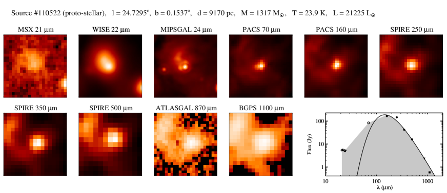
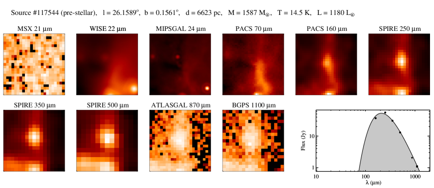
Figure 2: Multi-wavelength $2\arcmin\times 2\arcmin$ images of two sources listed in our catalogue, to provide an example of a proto-stellar (upper 11 panels) and a pre-stellar source (lower 11 panels). The source coordinates and physical properties are reported above each set of panels. For each source position ten images at 21, 22, 24, 70, 160, 250, 350, 500, 870, and 1100 $\mu$m, taken from the survey indicated in the title, are shown (the colour scale is logarithmic, in arbitrary units). Finally, the SED of each of the two sources is shown: filled and open symbols indicate fluxes which are taken into account or not, respectively, for the grey body fit (solid line, see Section 4). The grey-shaded area is a geometric representation of the integral calculated to estimate the source bolometric luminosity (see Sections 3.3 and 4).

To mitigate the first effect, we performed deeper, targeted extractions at PACS wavelengths towards two types of sources. One type consisted of “SPIRE-only” sources, i.e. sources clearly detected only at 250, 350 and 500 $\mu$m. Since SED fitting for such sources is poorly constrained, a further extraction at 160 $\mu$m, deeper than that of Molinari et al. (2016a), was required in order to set at least an upper limit for the flux shortwards of what could be the peak of the SED. In this way, 9705 further detections and 9992 upper limits at 160 $\mu$m were recovered.

The second type of sources consists of those showing a 160 $\mu$m counterpart (original or found after deeper search) but no detection at 70 $\mu$m. To ascertain that the starless nature of these objects is not assigned simply due to a failure of the source detection process, we performed a deeper search for a 70 $\mu$m counterpart toward those targets: in this way, a possible clear counterpart not originally listed in the single band catalogues would allow us to label the object as proto-stellar. Adopting this strategy, 912 further detections and 76215 upper limits at 70 $\mu$m were recovered.

Whereas the proto-stellar objects are expected to host ongoing star formation, the relation between starless objects and star formation processes must be further examined, since only gravitationally bound sources fulfil the conditions for a possible future collapse. Here we use the so-called “Larson’s third relation” to assess if an object can be considered bound: the condition we impose involves the source mass, $M$, and radius, $r$ (see Sections 4 and 6), and is formulated as $M(r)>460M_{\odot}(\mathrm{r}/\mathrm{pc})^{1.9}$ (Larson, 1981). Masses above this threshold identify bound objects, i.e. genuine pre-stellar aggregates.

In Table 1 the statistics of the sources of the catalogue, divided into proto-stellar, pre-stellar and starless unbound, is reported, while in Figure 2 the SEDs and the corresponding grey-body fits are shown for one proto-stellar and one pre-stellar source, for the sake of example. More details and a discussion about the proto- to pre-stellar source ratio are given in Section 8.1.

One of the aims of this paper is to show the amount of information that can be extracted simply from continuum observations in the FIR/sub-mm, combining Hi-GAL data with other surveys in adjacent wavelength bands and using spectroscopic data only to obtain kinematic distances. On the one hand, for many sources, these data can be complemented with line observations to obtain a more detailed picture. On the other hand, Hi-GAL produced an unprecedentedly large and unbiased catalogue containing many thousands of newly detected cold clumps, for which it is important to provide a first classification. The criteria we provide to separate different populations, although somewhat conventional in the Herschel literature, remain probably too clear-cut and surely affected by biases we introduced in this section and discuss also in the following sections of this paper. Reciprocal contamination of the samples certainly increases overlap of the physical property distributions obtained separately for the different populations, as will be seen in Sections 6 and 7.

Table 1: Number of sources in the Hi-GAL catalog, in ranges of longitude.

Longitude range	Proto-stellar		Highly-reliable Starless (Pre-stellar)		Poorly-reliable Starless (Pre-stellar)		Total
	w/ distance	w/o distance	w/ distance	w/o distance	w/ distance	w/o distance
$-71^{\circ}\leq\ell<-20^{\circ}$	8227	1425	10384 (9598)	2978 (2265)	10696 (7531)	3321 (1519)	37031
$-20^{\circ}\leq\ell<-10^{\circ}$	1752	273	2667 (2506)	611 (537)	2548 (1855)	591 (345)	8442
$-10^{\circ}\leq\ell<0^{\circ}$	0	2154	0 (0)	3357 (3139)	0 (0)	3417 (2544)	8928
$0^{\circ}\leq\ell<19^{\circ}$	505	3165	398 (380)	5689 (5271)	318 (249)	5488 (4053)	15563
$19^{\circ}\leq\ell<33^{\circ}$	2646	549	3172 (2893)	1260 (1068)	3045 (2200)	1312 (832)	11984
$33^{\circ}\leq\ell<67^{\circ}$	2704	1184	4189 (3818)	3149 (2548)	3814 (2520)	3934 (2000)	18974
Total	15834	8750	20810 (19195)	17044 (14828)	20421 (14355)	18063 (11293)	100922

4 SED fitting

Once the SEDs of all entries in the filtered catalogue are built by assembling the photometric information as explained above, it is possible to fit a single grey body function to its $\lambda\geq 160$ $\mu$m portion, and therefore derive the mass $M$ and the temperature $T$ of the cold dust in those objects.

Many details on the use of the grey body to model FIR SEDs have been provided and discussed by Elia & Pezzuto (2016). Here we report only concepts and analytic expressions which are appropriate for the present paper. The most complete expression for the grey body explicitly contains the optical depth:

$$F_{\nu}=(1-\mathrm{e}^{-\tau_{\nu}})B_{\nu}(T_{d})\Omega~{},$$ (1)

recently used, e.g., in Giannini et al. (2012), where $F_{\nu}$ is the observed flux density at the frequency $\nu$, $B_{\nu}(T_{d})$ is the Planck function at the dust temperature $T_{d}$ and $\Omega$ is the source solid angle in the sky. The optical depth can be parametrised in turn as

$$\tau_{\nu}=(\nu/\nu_{0})^{\beta}~{},$$ (2)

where the cut-off frequency $\nu_{0}=c/\lambda_{0}$ is such that $\tau_{\nu_{0}}=1$, and $\beta$ is the exponent of the power-law dust emissivity at large wavelengths. After constraining $\beta=2$, as typically adopted also in the Gould Belt (e.g., Könyves et al., 2015) and HOBYS (e.g., Giannini et al., 2012) consortia, and as recommended by Sadavoy et al. (2013), and $\Omega$ to be equal to the source area as measured by CuTEx at the reference wavelength of 250 $\mu$m (cf. Elia et al., 2013), the free parameters of the fit remain $T$ and $\lambda_{0}$. For these parameters we explored the ranges 5 K $\leq T\leq$ 40 K and $5~{}\mu$m $\leq\lambda_{0}\leq~{}350~{}\mu$m, respectively.

The clump mass does not appear explicitly in Equation 1 but can be derived from

$$M=(d^{2}\Omega/\kappa_{\mathrm{ref}})\tau_{\mathrm{ref}}~{},$$ (3)

as shown by Pezzuto et al. (2012), where $\kappa_{\mathrm{ref}}$ and $\tau_{\mathrm{ref}}$ are the opacity and the optical depth, respectively, estimated at a given reference wavelength $\lambda_{\mathrm{ref}}$. To preserve the compatibility with previous works based on other Herschel key-projects (e.g. Könyves et al., 2010; Giannini et al., 2012) here we decided to adopt $\kappa_{\mathrm{ref}}=0.1$ cm² g^-1 at $\lambda_{\mathrm{ref}}=300~{}\mu$m (Beckwith et al., 1990, already accounting for a gas-to-dust ratio of 100), while $\tau_{\mathrm{ref}}$ can be derived from Equation 2. The choice of $\kappa_{\mathrm{ref}}$ constitutes a critical point (Martin et al., 2012; Deharveng et al., 2012), thus it is interesting to show how much the mass would change if another estimate of $\kappa_{\mathrm{ref}}$ were adopted. The dust opacity at $300~{}\mu$m from the widely used OH5 model (Ossenkopf & Henning, 1994) is $\kappa_{300}=0.13$ cm² g^-1, which would produce a 30% underestimation of masses with respect to our case. Preibisch et al. (1993) quote $\kappa_{1300}=0.005$ cm² g^-1 which, for $\beta=2$, would correspond to $\kappa_{300}=0.094$ cm² g^-1, implying a $\sim 6\%$ larger mass. Similarly, the value of Netterfield et al. (2009), $\kappa_{250}=0.16$ cm² g^-1, would translate to $\kappa_{300}=0.11$ cm² g^-1, practically consistent with the value adopted here. However, further literature values of $\kappa_{250}$ quoted by Netterfield et al. (2009) in their Table 3, span an order of magnitude, from $\kappa_{250}=0.024$ cm² g^-1(Draine & Li, 2007) to $\kappa_{250}=0.22-0.25$ cm² g^-1(Ossenkopf & Henning, 1994), which would lead to a factor from 6 to 0.6 on the masses calculated in this paper.

For very low values of $\lambda_{0}$ (i.e. much shorter than the minimum of the range we consider for the fit, namely $160~{}\mu$m) the grey body has a negligible optical depth at the considered wavelengths, so that Equation 1 can be simplified as follows:

$$F_{\nu}=\frac{M\kappa_{\mathrm{ref}}}{d^{2}}\left(\dfrac{\nu}{\nu_{\mathrm{ref}}}\right)^{\beta}B_{\nu}(T_{d})~{}.$$ (4)

(cf. Elia et al., 2010). We note that the estimate of $\lambda_{0}$ does not affect our results significantly when it implies $\tau\leq 0.1$ at $160~{}\mu$m. According to Equation 2 and for $\beta=2$, we find that the critical value is encountered for $\lambda_{0}\sim 50.6~{}\mu$m. If the fit procedure using Equation 1 provides a $\lambda_{0}$ value shorter than that, the fit is repeated based on Equation 4, and the mass and temperature computed in this alternative way are considered as the definitive estimates of these quantities for that source. In Figure 3 we show how the temperature and mass values obtained through Equations 1 ($T_{\mathrm{tk}},M_{\mathrm{tk}}$) and 4 ($T_{\mathrm{tn}},M_{\mathrm{tn}}$) appear generally equivalent as long as $\lambda_{0}$ (obtained through the former) is much shorter than $160~{}\mu$m (say $\lambda<100~{}\mu$m), since both models have extremely low (or zero) opacities at the wavelengths involved in the fit. Quantitatively speaking, the average and standard deviation of the $T_{tk}/T_{tn}$ ratio for $\lambda<160~{}\mu$m are 1.01 and 0.02, respectively. However, an increasing discrepancy is visible at increasing $\lambda_{0}$, highlighting the tendency of Equation 4 to underestimate the temperature and to overestimate the mass.

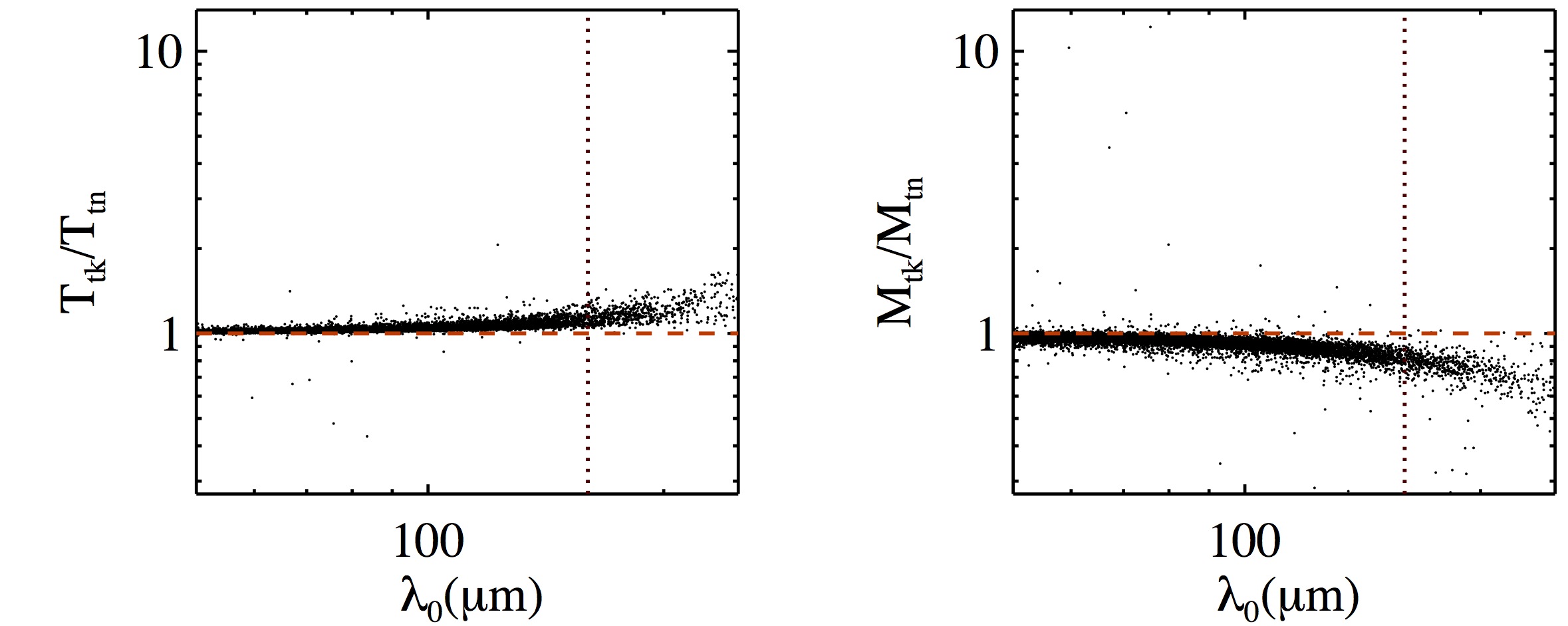
Figure 3: Left: Ratio of the dust temperatures derived by fitting Equations 1 and 4 to SEDs (and denoted here with $T_{\mathrm{tk}}$ and $T_{\mathrm{tn}}$, to indicate an optically “thick” and thin regime, respectively) vs the corresponding $\lambda_{0}$ obtained through Equation 1. The $x$-axis starts from $50.6~{}\mu$m, corresponding to the minimum value for which this comparison makes sense (see text). The $\lambda_{0}=160~{}\mu$m value is highlighted as a reference with a vertical dotted line. The red dashed line represents the $T_{\mathrm{tk}}=T_{\mathrm{tn}}$ condition. Right: the same as left panel, but for the masses $M_{\mathrm{tk}}$ and $M_{\mathrm{tn}}$ derived through Equations 3 and 4, respectively.

SED fitting is performed by $\chi^{2}$ optimization of a grey body model on a grid that is refined in successive iterations to converge on the final result. The strategy of generating a SED grid to be compared with data also gives us the advantage of applying PACS colour corrections directly to the model SEDs (since its temperature is known for each of them), rather than correcting the data iteratively (cf. Giannini et al., 2012).

For sources with no assigned distance, a virtual value of 1 kpc was assumed, to allow the fit anyway and distance-independent quantities (such as $T$) to be derived, and also distance-independent combinations of single distance-dependent quantities (as $L_{\mathrm{bol}}/M$, see Section 6.5).

The luminosity of the starless objects was estimated using the area under the best fitting grey body. For proto-stellar objects, however, the luminosity was calculated by summing two contributions: the area under the best fitting grey body starting from 160 $\mu$m and longward, plus the area of the observed SED between 21 and 160 $\mu$m counterparts (if any) to account for MIR emission contribution exceeding the grey body.

5 Summary of the creation of the scientific catalogue

The generation of the catalogue used for the scientific analysis presented in this paper can be summarised as follows:

1. Select the sources located in regions observed with both PACS and SPIRE.

2. Perform positional band-merging of single band catalogues. At the first step, the single-band catalogue at 500 $\mu$m is taken, and the closest counterpart in the 350 $\mu$m image, if available, is assigned. The same is repeatedly done for shorter wavelengths, up to 70 $\mu$m. The ellipse describing the object at the longer wavelength is chosen as the matching region.

3. Select sources in the band-merged catalogue that have counterparts in at least three contiguous Herschel bands (except the 70 $\mu$m) and show a “regular” SED (with no cavities and not increasing toward longer wavelengths).

4. Find counterparts at MIR and mm wavelengths for all entries in the band-merged and filtered catalogue. Shortwards of 70 $\mu$m catalogues at 21, 22, and 24 $\mu$m were searched and the corresponding flux reported is the sum of all objects falling in the ellipse at 250 $\mu$m. Longwards of 500 $\mu$m counterparts where searched by mining 870 $\mu$m ATLASGAL public data, or extracting sources through CuTEx, as well as 1.1 mm BGPS data.

5. Fill the catalogue where fluxes at 160 and/or at 70 $\mu$m were missing, to improve the the quality of labelling sources as starless or proto-stellar (see next step).

6. Move the selected SEDs which remain with only three fluxes in the five Hi-GAL bands to a list of sources with, on average, barely-reliable physical parameter estimation.

7. Classify sources as proto-stellar or starless, depending on presence or lack of a detection at 70 $\mu$m, respectively.

8. Assign a distance to all sources using the method described in Russeil et al. (2011).

9. Fit a grey body to the SED at $\lambda\geq 160~{}\mu$m to derive the envelope average temperature, and, for sources provided with a distance estimate, the mass and the luminosity.

10. Make a further classification, among starless sources, between gravitationally unbound or bound (pre-stellar) sources, based on the mass threshold suggested by the Larson’s third law.

The catalogue, generated as described above and constituted by two lists (“high reliability” and “low reliability”, respectively), is available for download at http://vialactea.iaps.inaf.it/vialactea/public/HiGAL_clump_catalogue_v1.tar.gz.

The description of the columns is reported in Appendix A.

6 Results

6.1 Physical size

For a source population distributed throughout the Galactic plane at an extremely wide range of heliocentric distances, as in our case, it is fundamental to consider the effective size of these compact objects (i.e. detected within a limited range of angular sizes) in order to assess their nature.

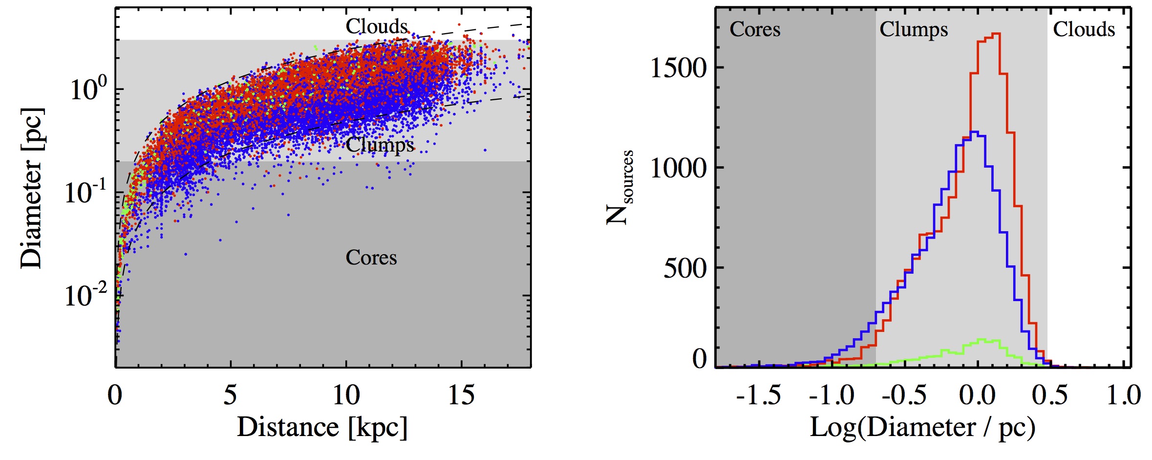
Figure 4: Left: Hi-GAL clump linear diameters, estimated at 250 $\mu$m, vs distances (blue: proto-stellar; red: pre-stellar; green: starless unbound). Different background levels of grey indicate size ranges corresponding to different object typologies (see text). The upper and lower dashed lines represent an angular size of 50$\arcsec$ and 10$\arcsec$, respectively. Right: Distribution of source diameters for proto-stellar, pre-stellar, and starless unbound sources. Line and background colours are the same as in the left panel.

Sure enough, we can derive the linear sizes only for objects with a distance estimate, starting from the angular size estimated at the reference wavelength of 250 $\mu$m as the circularised and deconvolved size of the ellipse estimated by CuTEx. In Figure 4, left panel, we show the relation between the physical diameter and the distance for these sources, highlighting how this quantity is given by the combination of the source angular size and its distance. Given the large spread in distance, a wide range of linear sizes is found, corresponding to very different classes of ISM structures.

In Figure 4, right panel, we provide the histogram of the diameter $D$ separately for the proto-stellar, pre-stellar and starless unbound sources, using the subdivision scheme proposed by Bergin & Tafalla (2007) (cores for $D<0.2$ pc, clumps for $0.2\geq D\leq 3$ pc, and clouds for $D>3$ pc, although the natural transition between two adjacent classes is far from being so sharp) to highlight how only a small portion of the Hi-GAL compact sources is compatible with a core classification, while most of them are actually clumps. A very small fraction of sources, corresponding to the most distant cases, can be considered as entire clouds. However, given the dominance of the clump-sized sources, is practical to refer to the sources of the present catalogue with the general term “clumps”. The underlying, generally inhomogeneous substructure of these clumps is not resolved in our observations, but it can reasonably supposed that they are composed by a certain number of cores and by inter-core diffuse medium (e.g., Merello et al., 2015) so that, in the proto-stellar cases, we generally should not expect to observe the formation process of a single protostar, but rather of a proto-cluster.

We note that the histograms in Figure 4, right panel, should not be taken as a coherent size distribution of our source sample, due to the underlying spread in distance. It is not possible, therefore, to make global comparisons between the different classes as, for example, in Giannini et al. (2012) who considered objects from a single region, all located at the same heliocentric distance. The same consideration applies to the distribution of other distance-dependent quantities.

6.2 Dust temperature

The distributions of grey body temperatures of the sources are shown in Figure 5. As already found by Giannini et al. (2012), Elia et al. (2013), Giannetti et al. (2013), Veneziani et al. (2017) through Hi-GAL observations but also by Olmi et al. (2009) through BLAST observations, the distributions of pre- and proto-stellar sources show some relevant differences, the latter being found towards warmer temperatures with respect to the former. A quantitative argument is represented by the average values $\bar{T}_{\mathrm{pre}}=12.0$ K and $\bar{T}_{\mathrm{prt}}=16.0$ K for pre- and proto-stellar sources, and the median values $\tilde{T}_{\mathrm{pre}}=11.7$ K and $\tilde{T}_{\mathrm{prt}}=15.1$ K, respectively.

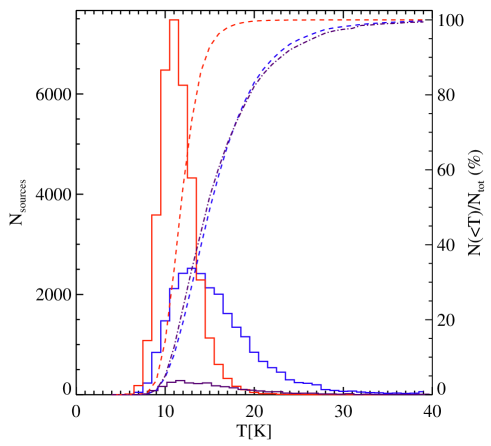
Figure 5: Grey body temperature distributions for the pre- (red histogram) and proto-stellar (blue histogram) sources considered for science analysis in this paper. Cumulative curves of the same distributions are also plotted as dashed lines (and the same colours), according to the $y$-axis on the right side of the plot. Finally, the temperature distribution of the sub-sample of MIR-dark proto-stellar sources is plotted in dark purple, and the corresponding cumulative as a dotted-dashed dark purple line.

Furthermore, both the temperature distributions seem quite asymmetric, with a prominent high-temperature tail. This can be seen by means of the skewness indicator (defined as $\gamma=\mu_{3}/\sigma^{3}$, where $\mu_{3}$ is the third central moment and $\sigma$ the standard deviation) of the two distributions: $\gamma_{\mathrm{pre}}=1.06$ and $\gamma_{\mathrm{prt}}=1.40$, respectively. The positive skew, in this case, indicates that the right tail is longer ($\gamma=0$ for a normal distribution), and quantifies that. On the other hand, the pre-stellar distribution appears more peaked than the proto-stellar one. The kurtosis of a distribution, defined as $\delta=\mu_{4}/\sigma^{4}$ (where $\mu_{4}$ is the fourth central moment), is useful to quantify the level of peakedness (for a normal distribution, $\delta=3$). In these two cases the kurtosis values are found to be quite different for the two distributions ($\delta_{\mathrm{pre}}=3.67$ and $\delta_{\mathrm{prt}}=3.04$, respectively). Finally, we also plot the cumulative distributions of the temperatures, which is another way to highlight the behaviours examined so far. We find that $99\%$ of the pre-stellar (proto-stellar) sources have dust temperatures lower than $18.1$ K (33.1 K), and the temperature range widths required to go from 1% to 99% levels are 9.9 K and 24.2 K, respectively.

The differences found between the two distributions are even more meaningful from the point of view of the separation between the two classes of sources, if one keeps in mind that the temperature is estimated from data at wavelengths longer than $160~{}\mu$m, hence independently from the existence of a measurement at $70~{}\mu$m, which discriminates between proto-stellar and starless sources in our case.

These findings can be regarded from the evolutionary point of view: while pre-stellar sources represent the very early stage (or “zero” stage) of star formation and, as such, are characterised by very similar temperatures, proto-stellar sources are increasingly warmer as the star formation progresses in their interior (e.g., Battersby et al., 2010; Svoboda et al., 2016), so that the spanned temperature range is larger and skewed towards higher values. A prominent high-temperature tail should be regarded, in this sense, as a signature of a more evolved stage of star formation activity.

To corroborate this view, we consider the temperatures of the sub-sample of proto-stellar sources of our catalogue lacking a detection in the MIR (i.e. at 21 and/or 22 and/or 24 $\mu$m, hereafter MIR-dark sources, as opposed to MIR-bright), whose distribution is also shown in Figure 5. They represent 10% of the total proto-stellar sources (therefore dominated by MIR-bright cases). The average and median temperature for this class of objects are $\bar{T}_{\mathrm{Md}}=16.0$ K and $\tilde{T}_{\mathrm{Md}}=14.8$ K, respectively, i.e. halfway between the values found for pre-stellar sources and those for the whole sample of proto-stellar ones, which is dominated by MIR-bright sources.

The reader should be aware that the dust temperature discussed here is simply derived from the grey-body fit of the SED at $\lambda\geq 160~{}\mu$m and represents an estimate of the average temperature of the cold dust in the clump. Using line tracers it is possible to probe the kinetic temperature of warmer environments, such as the inner part of proto-stellar clumps, which is typically warmer ($T>20$ K, e.g. Molinari et al., 2016b; Svoboda et al., 2016) than the median temperature found here for this class of sources. Despite of this, as seen in this section, the grey body temperature can help to infer the source evolutionary stage, and turns out to be particularly efficient in combination with other parameters, as further discussed in Section 7.

6.2.1 Herschel colours and temperature

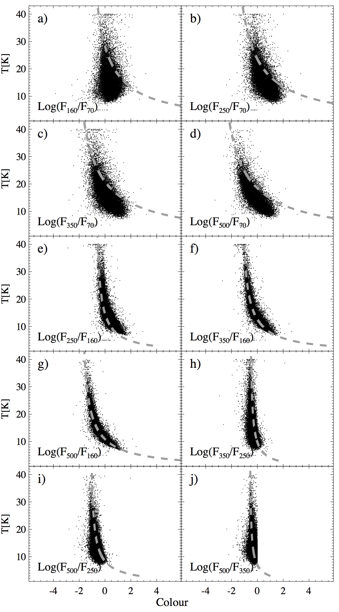
Figure 6: Panels $a$-$j$: plots of source temperature (as derived through the grey body fit) vs all colours obtainable from possible pair combinations of the five Hi-GAL wavebands. Each plot is obtained using all sources provided with fluxes at the two involved wavelengths, specified at the bottom of the panel. The unnatural vertical cut of the point distribution in panel $j$ is an artefact due to one of the filters adopted for source selection, ruling out sources with $F_{350}<F_{500}$ (rescaled fluxed are considered, see Section 3.1). The grey dashed line represents the temperature of a grey body with $\beta=2$.

The availability of dust temperatures derived from grey body fits makes it possible to directly compare with Herschel colours (cf. Elia et al., 2010; Spezzi et al., 2013), to ascertain which ones are better representative of the temperature. In Figure 6 the source temperature is plotted vs the ten possible colour pairs that can be obtained by combining the five Herschel bands (for each combination, only sources detected at both wavelengths are displayed). We designate as colour the decimal logarithm of the ratio of fluxes at two different wavelengths. Since the 70 $\mu$m band is not involved in the temperature determination, the colours built from it (plots $a$ to $d$) do not show any tight correlation with temperature, while for the remaining six colours such correlation appears more evident, especially for those colours involving the 160 $\mu$m band. The best combination of spread of colour values (which decreases the level of temperature degeneracy, mostly at low temperatures) and agreement with the analytic behaviour expected for a grey body is found for colours involving the flux at $160~{}\mu$m (panels $e$, $f$, and $g$). In particular, for the $F_{500}/F_{160}$ colour the grey body curve has the shallowest slope, so that we propose this colour as the most suitable diagnostics of the average temperature in the absence of a complete grey body fit. For the case of SPIRE-only sources, lacking a counterpart at 160 $\mu$m, only three colours are available but their relation with dust temperature (cf. panels from $h$ to $j$) appears to be affected by a high degree of degeneracy, making these colours unreliable temperature indicators.

6.3 Mass and surface density

Once source masses are obtained, it would be straightforward to show and analyse the resulting distribution (clump mass function, hereafter ClumpMF). However, since such discussion implies considerations about the clump mass-size relation and, somehow equivalently, the surface density, we postpone the analysis of the ClumpMF until the end of this section, after having dealt with those preparatory aspects.

A meaningful combination of source properties is represented by the mass $M$ vs radius $r$ diagram, which has been shown to be a powerful tool for investigating gravitational stability of Herschel compact sources, and their potential ability to form massive stars (André et al., 2010; Giannini et al., 2012; Elia et al., 2013). In both cases, in fact, requirements expressed in terms of surface density threshold can be translated into a simple mass-radius relation. Figure 7 shows the mass vs radius distribution for the sources analyzed in the present study. In the top left panel the starless sources are shown while, to avoid confusion, the proto-stellar ones are reported in the top-right panel: the Larson’s relation mentioned in Section 3.5 is plotted to separate the starless bound (pre-stellar) and unbound sources.

From this plot it is possible to determine if a given source satisfies the condition for massive star formation to occur, where such condition is expressed as surface density, $\Sigma$, threshold. Krumholz & McKee (2008) established a critical value of $\Sigma_{\mathrm{crit}}=1$ g cm^-2 based on theoretical arguments. However López-Sepulcre et al. (2010) and Butler & Tan (2012), based on observational evidences, suggest the less severe values of $\Sigma_{\mathrm{crit}}=0.3$ and $0.2$ g cm^-2, respectively. Also, Kauffmann & Pillai (2010), based on empirical arguments, propose the threshold $M(r)>870~{}M_{\odot}(\mathrm{r}/\mathrm{pc})^{1.33}$ as minimum condition for massive star formation. Finally, the recent analysis by Baldeschi et al. (2017) of the distance bias affecting the source classification according to the two aforementioned thresholds, produced the further criterion $M(r)>1282~{}M_{\odot}(\mathrm{r}/\mathrm{pc})^{1.42}$. In the upper side we represent the most (Krumholz & McKee, 2008) and the least (Kauffmann & Pillai, 2010) demanding thresholds, respectively, to allow comparison with the behaviour of our catalogue sources.

As reported in Table 2, a remarkable fraction of sources appears to be compatible with massive star formation based on the three thresholds (defined as $\Sigma_{\mathrm{KM}}$, $\Sigma_{\mathrm{B}}$, and $\Sigma_{\mathrm{KP}}$, respectively), especially the last. This is further highlighted by the bottom-left panel of Figure 7, which summarises the previous two panels reporting the source densities for both the pre- and the proto-stellar source populations. The peak of the proto-stellar source concentration lies well inside the area delineated by the Kauffmann & Pillai (2010) relation, while the pre-stellar distribution peaks at smaller densities. Rigorously speaking, however, such considerations on the initial conditions for star formation should be applied only to the pre-stellar clumps, since in the proto-stellar ones part of the initial clump mass has been already transferred onto the forming star(s) or dissipated under the action of stellar radiation pressure or through jet ejection. In any case, the presence of a significant number of very dense pre-stellar sources translates into an interestingly large sample of targets for subsequent study of the initial conditions for massive star formation throughout the Galactic plane (see Section 8.1). For such sources, due to contamination between the two classes described in Section 3.5, a further and deeper analysis is requested to ascertain their real starless status, independently from the lack of a Herschel detection at $70~{}\mu$m.

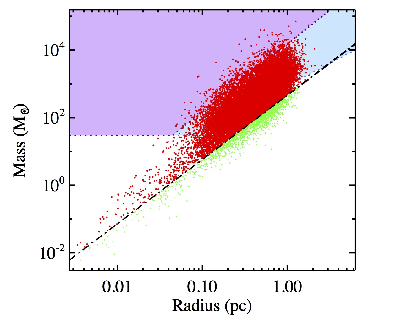
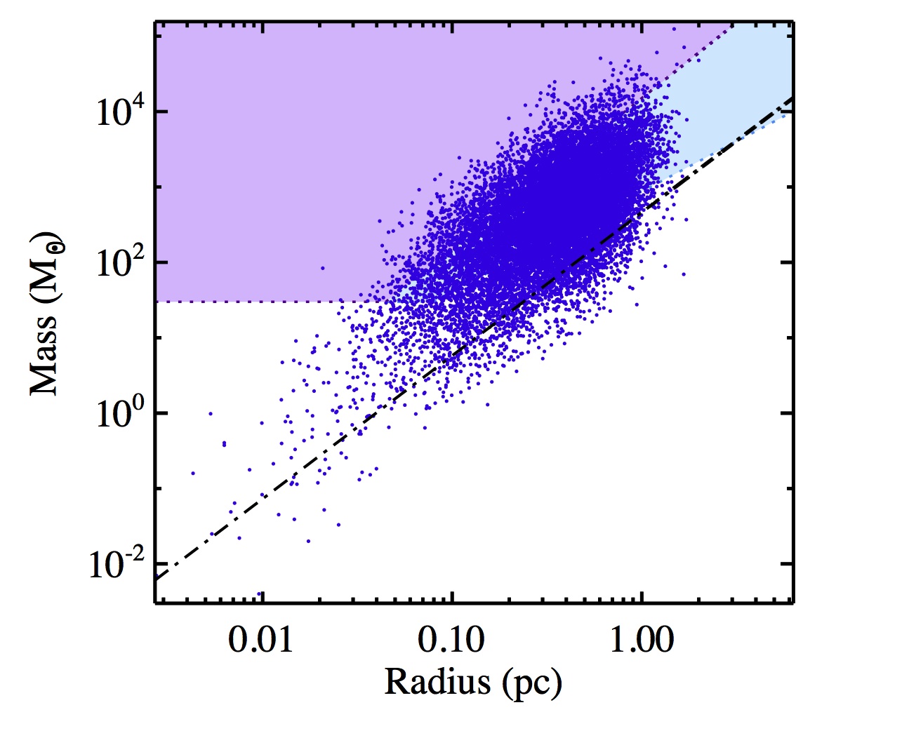
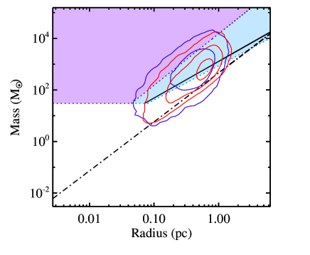
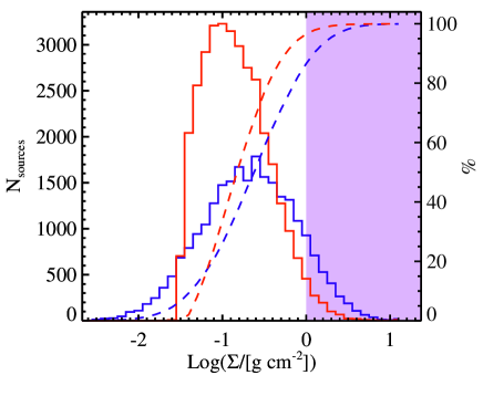
Figure 7: Top left: Mass vs radius plot for starless sources. Pre-stellar (red) and starless (green) sources are separated by the line $M(r)=460~{}M_{\odot}~{}(r/\mathrm{pc})^{1.9}$ (Larson, 1981) (dotted dashed black line), see Section 3.5. The areas of the mass-radius plane corresponding to combinations fulfilling the Kauffmann & Pillai (2010) and the Krumholz & McKee (2008) thresholds for compatibility with high-mass star formation are filled with light blue and purple, respectively, the latter being contained in the former, and both delimited by a darker dotted line. Notice that, adopting a lower limit of $10~{}M_{\odot}$ for the definition of massive star, and a star formation efficiency factor of $1/3$ for the core-to-star mass transfer as in Elia et al. (2013), these zones can not extend below $30~{}M_{\odot}$. Top right: the same as in top left panel, but for proto-stellar sources. Bottom left: source density isocontours representing the pre- and proto-stellar distributions displayed in the two upper panels of this figure. Densities have been computed subdividing the area of the plot in a grid of $70\times 70$ cells; once the global maxima for both distributions have been found, the plotted contours represent the 2%, 20% and 70% of the largest of those two peak values, so that the considered levels correspond to the same values for both distributions, to be directly comparable. The black solid line crossing the bottom part of the light blue area represents the threshold of Baldeschi et al. (2017). Bottom right: surface density distributions (solid histograms) for pre- (red) and proto-stellar (blue) sources. Because surface density is a distance-independent quantity, all sources (with and without distance estimates) are taken into account to build these distributions. The cumulative curves are plotted with dashed lines, normalised to the $y$-axis scale on the right. The zone corresponding to densities surpassing the Krumholz & McKee (2008) threshold is filled with purple colour.

Notice that the fractions corresponding to the threshold of Kauffmann & Pillai (2010) reported in Table 2 appear remarkably lower than the same quantity estimated by Wienen et al. (2015) for the ATLASGAL catalogue, namely 92%. This discrepancy cannot be simply explained by the better sensitivity of Hi-GAL: taking the sensitivity curve in the mass vs radius of Wienen et al. (2015, their Figure 23), we find that the majority of our sources lie above that curve. The main reason, instead, resides in the analytic form itself of the adopted threshold. As mentioned above, Baldeschi et al. (2017) shown that, even in presence of dilution effects due to distance, sources in the mass vs radius plot are found to follow a slope steeper than the exponent 1.33, so that large physical radii, typically associated to sources observed at very far distances, correspond to masses larger than the Kauffmann & Pillai (2010) power law. This is not particularly evident in our Figure 7 since the largest probed radii are around 1 pc, and the large spread of temperatures makes the plot quite scattered. Instead, Figure 23 of Wienen et al. (2015) contains a narrower distribution of points (since masses were derived in correspondence with only two temperatures, both higher than 20 K), extending up to $r\simeq 6$ pc: at $r\gtrsim 1$ pc almost the totality of sources satisfy the Kauffmann & Pillai (2010) relation. Clearly, another contribution to this discrepancy can be given by the scatter produced by possible inaccurate assignment of the far kinematic distance solution in cases of unsolved ambiguity (see Section 3.4).

Table 2: Hi-GAL sources with mass-radius relation compatible with massive star formation according to surface density thresholds $\Sigma_{\mathrm{KP}}$, $\Sigma_{\mathrm{B}}$, and $\Sigma_{\mathrm{KM}}$ (see text).

	$\Sigma>\Sigma_{\mathrm{KP}}$		$\Sigma>\Sigma_{\mathrm{B}}$		$\Sigma>\Sigma_{\mathrm{KM}}$
	counts	%	counts	%	counts	%
Proto-stellar	11210	71.3	10012	63.7	2062	13.1
Pre-stellar	12431	64.8	9973	52.0	546	2.8

The information contained in the mass-radius plot can be rearranged in a histogram of the surface density $\Sigma$ such as that in Figure 7, bottom right. The pre-stellar source distribution presents a sharp artificial drop at small densities due to the removal of the unbound sources which is operated along $M\propto r^{1.9}$, i.e. at an almost constant surface density ($M\propto r^{2}$). Instead, despite the considered pre-stellar population being globally more numerous than the proto-stellar one, at high densities ($\Sigma\gtrsim 1$ g cm^-2) the latter prevails over the former. The proto-stellar distribution, in general, appears shifted towards larger densities, compared with the pre-stellar one, as can be seen in the different behaviour of the cumulative curves, also shown in figure. This evidence is in agreement with the result of He et al. (2015), based on the MALT90 survey. Further evolutionary implications will be discussed in Section 7.3.

We note, as discussed in Section 6.1, that the compact sources we consider may correspond, depending on their heliocentric distance, to large and in-homogeneous clumps with a complex underlying morphology not resolved with Herschel. On the one hand, this implies that the global properties we assign to each source do not remain necessarily constant throughout its internal structure, thus a source fulfilling a given threshold on the surface density might, in fact, contain sub-critical regions. On the other hand, in a source with a global sub-critical density, super-critical portions might actually be present, leading to mis-classifications; for this reason the numbers reported in Table 2 should be taken as lower limits.

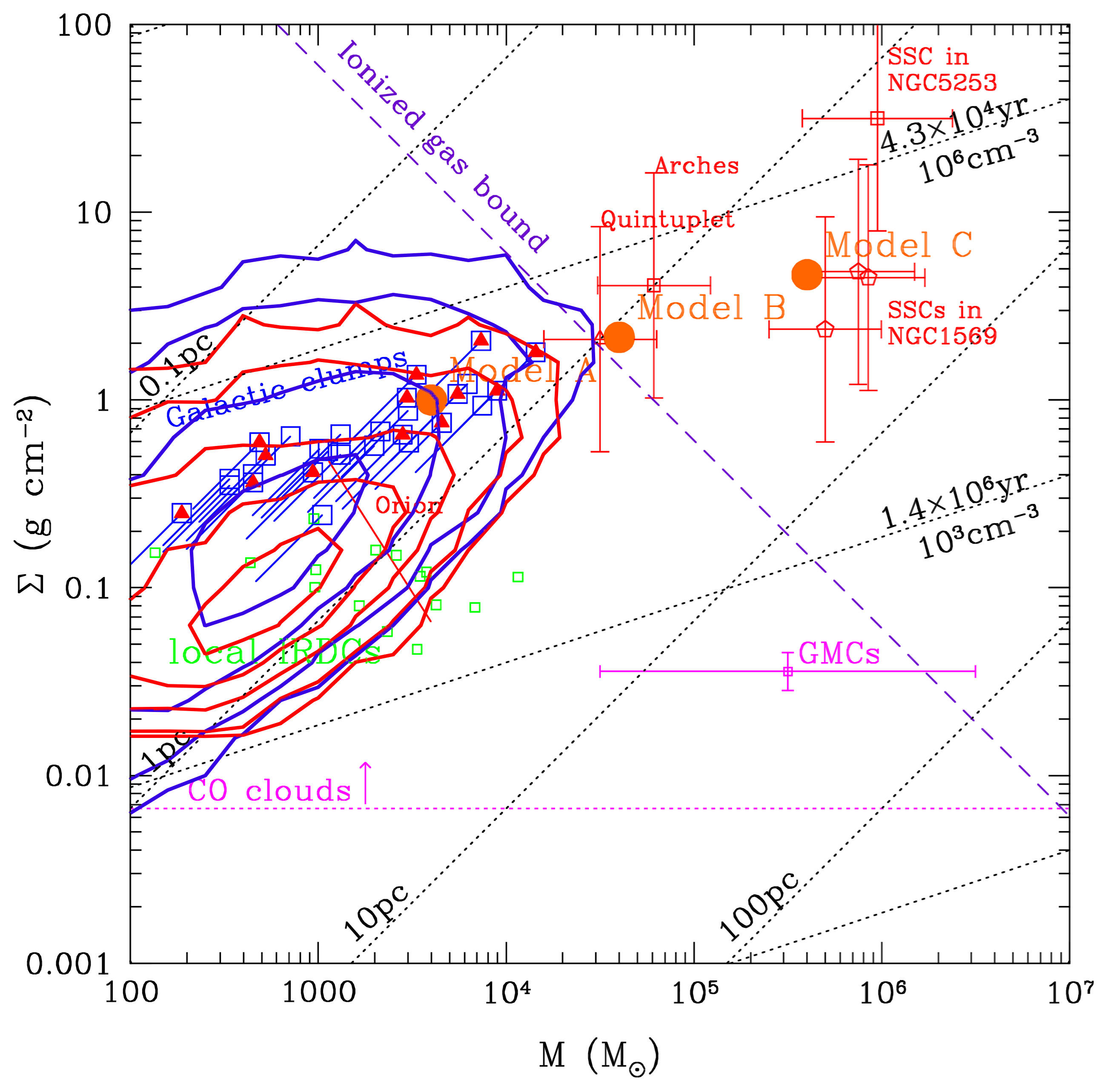
Figure 8: Plot of surface density vs mass of Tan (2005, his Figure 1), with overplotted number density contours of pre- (red) and proto-stellar (blue) sources of our catalogue. The source density is computed in bins of 0.2 in decimal logarithm, and contour levels are 5, 20, 100, 250, and 500 sources per bin. The horizontal cut at lowest densities for red contours is due to the removal of starless unbound sources. The diagonal dotted lines represent the locii of given radii and number densities (and corresponding free-fall times). Typical ranges for molecular clouds are indicated with magenta lines, while the condition for the ionised gas to remain bound is indicated by the blue dashed line. Finally, locations for a selection of IRDCs (green squares), dense star-forming clumps (blue squares), massive clusters (red symbols) and cluster models of Tan (2005) (filled orange circles). More details about additional information reported in this diagram are provided in Tan (2005) and Molinari et al. (2014, their Figure 11).

We use the collected information about source masses and surface densities to place them in the $\Sigma$ vs $M$ plot of Tan (2005), in which different classes of structures populate different regions. Our Figure 8 is analogous to Figure 11 of Molinari et al. (2014), but the “temporary” data set used for that plot is replaced here with the values from the final Hi-GAL physical catalogue. The Hi-GAL sources are found to lie in the regions quoted by Tan (2005) for Galactic clumps and local IRDCs. In the upper-right part of their distribution they graze the line representing the condition for ionised gas to remain bound. This plot summarises the nature of the sources in our catalogue: clumps spanning a wide range of mass/surface density combinations, with many of them found to be compatible with the formation of massive Galactic clusters.

6.4 The ClumpMF

The ClumpMF is an observable that has been extensively studied for understanding the connection between star formation and parental cloud conditions. Although formulations are quite similar, the ClumpMF should not be confused with the core mass function (hereafter CoreMF), typically studied in nearby star forming regions ($d\lesssim 1$ kpc). Differences between these two distributions will be discussed later in this section.

Large infra-red/sub-mm surveys generated numerous estimates of the ClumpMF (e.g., Reid & Wilson, 2005, 2006; Eden et al., 2012; Tackenberg et al., 2012; Urquhart et al., 2014a; Moore et al., 2015). Likewise, data from Hi-GAL have been used for building the ClumpMF in selected regions of the Galactic plane (Olmi et al., 2013; Elia et al., 2013).

Building the mass function of a given sample of sources (Hi-GAL clumps in the present case) requires a sample to be defined in a consistent way. A clump mass function built from a sample of sources spanning a wide range of distances (as in our case) would be meaningless, since at large distances low-mass objects might not be detected or might be confused within larger, unresolved structures (see Appendix C), therefore it makes little sense to discuss it. Therefore, we first subdivide our source sample into bins of heliocentric distance, and then build the corresponding mass functions separately. In addition, as pointed out e.g. by Elia et al. (2013), it is more appropriate to build separate ClumpMFs for pre- and proto-stellar sources. Strictly speaking, only the mass distributions of pre-stellar sources is intrinsically coherent, as the mass of the proto-stellar sources does not represent the initial core mass, but rather a lower limit which depends on the current evolutionary stage of each source.

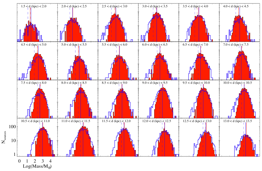
Figure 9: Clump mass function for pre-stellar (red filled histogram) and proto-stellar (blue histogram) sources, obtained in 0.5 kpc-wide heliocentric distance ranges. Each panel corresponds to the range which is reported in the upper part. Dashed red and blue line indicate the completeness limits, and solid red and blue vertical line indicate the lower limit used to fit the curves in Figure 10, for the pre- and proto-stellar case, respectively.

In Figure 9 the clump mass functions are shown. They have been calculated using sources provided with a distance estimate, from 1.5 to 13.5 kpc in distance bins of 0.5 kpc, in logarithmic mass bins, and separately for pre- and proto-stellar clumps.

It can be immediately noticed that, for any distance range, the proto-stellar ClumpMF is wider than the pre-stellar one, so that a deficit of pre-stellar clumps with respect to proto-stellar ones is seen both at lowest and highest masses in each bin of distance. The former effect is mostly due to sensitivity: sure enough, thanks to higher temperature, a proto-stellar source can be detected more easily than a pre-stellar source of the same mass. For example, according to Equation 7 in Appendix C.2, applied to a given mass, the flux of a source at $T=15$ K (i.e. $\sim\bar{T}_{\mathrm{prt}}$) is nearly twice that of a source at $T=12$ K (i.e. $\sim\bar{T}_{\mathrm{pre}}$ K). The latter effect can be in part explained with the pre-/proto-stellar possible blending and misclassification at increasing distance discussed in Appendix C, which leads to artificially overestimating the fraction of proto-stellar sources. However, from the quantitative point of view, this effect seems not sufficient to entirely account for the complete lack of pre-stellar sources as massive as the most massive proto-stellar ones. A further contribution is surely given as well by the more rapid evolution of massive pre-stellar sources towards the proto-stellar status (see, e.g., Motte et al., 2010b; Ragan et al., 2013). To correctly examine this point, sub-samples which are consistent in terms of heliocentric distance must be isolated, as we do in fact building Figure 9. Indeed, the structure of two clumps of, say, $200~{}M_{\odot}$ detected at $d=10$ kpc and $d=2$ kpc would be strongly different: the former would be expected to be likely composed of an underlying population of low-mass cores (Baldeschi et al., 2017), whereas the second, being better resolved by Herschel, would be denser and less fragmented than the former, therefore representing a more reliable candidate for hosting massive star formation and having shorter evolutionary time scales. This scenario is confirmed in most panels of Figure 9 where, given a range of heliocentric distances, a lack of pre-stellar clumps with respect to the proto-stellar ones is generally found in the bins corresponding to the highest masses present. Importantly, this indicates that it is not sufficient to simply claim that massive clumps have very short lifetimes (Ginsburg et al., 2012; Tackenberg et al., 2012; Csengeri et al., 2014): indeed, a large clump mass might also result from an associated large heliocentric distance, which implies multiple source confusion and inclusion of diffuse emission contaminating source photometry (see also Baldeschi et al., 2017). In this respect, clump density has to be taken into account as well, since only high densities ensure conditions for massive star formation and, therefore, for a faster evolution of a clump.

The differences observed between pre- and proto-stellar ClumpMFs are expected to be reflected on the slope of the power-law fit of high-mass end of these distributions, i.e. the usual way to extract information from the ClumpMF and compare it with the stellar initial mass function. The estimate of this slope is generally plagued by uncertainties due to arbitrary choice of mass bins and of the lower limit of the range to be involved in the fit. Olmi et al. (2013) have presented an efficient way, based on application of Bayesian statistics, to overcome such issues. Here we adopt a simpler approach:

• The slope of the ClumpMF is derived indirectly, by estimating the slope of the corresponding cumulative function defined, as a function of $M$, as the fraction of sources having mass larger than $M$. If a ClumpMF is calculated in logarithmic bins and is expected to have a power-law behaviour above a certain value $M_{\mathrm{fit}}$, so that $\mathrm{d}N(M)/\mathrm{d}\log_{10}(M)\propto M^{\alpha}$, then the corresponding cumulative function (hereafter CClumpMF) has the same exponent $\alpha$ (e.g., Shirley et al., 2003), and the estimate of such slope is independent from the bin used to sample the ClumpMF.

• The portion of the ClumpMF used in the fit should be delimited at bottom by the turn-over point of the ClumpMF $M_{\mathrm{peak}}$, namely the peak of a log-normal best fit (Chabrier, 2003). One has to ensure that this mass limit is larger than the completeness limit of the distribution. The estimation of the mass completeness limit $M_{\mathrm{compl}}$ is not trivial in our case, since multiple bands and variable temperature and distance concur in the mass determination, as discussed in Appendix C.2. Equation 7 can be applied to compute the limit, assuming the central distance of each bin, the median temperatures of pre- and proto-stellar sources, and a flux completeness limit at $350~{}\mu$m $F_{\mathrm{compl,350}}$ as estimated by Molinari et al. (2016a). This completeness limit, quoted by these authors as a function of Galactic longitude (their Figure 9), reaches a maximum of 13.08 Jy around $\ell=0^{\circ}$ (a region which does not provide sources for this analysis, given the lack of distance information), and a minimum of 0.65 Jy in the eastmost tile of the first quadrant. In intermediate regions, which provide the biggest contribution in building our ClumpMFs, in general $F_{\mathrm{compl,350}}\lesssim 4$ Jy, which we adopt here. In a few cases in which $M_{\mathrm{peak}}<M_{\mathrm{compl}}$, the latter is taken as the lower limit of the fit range.

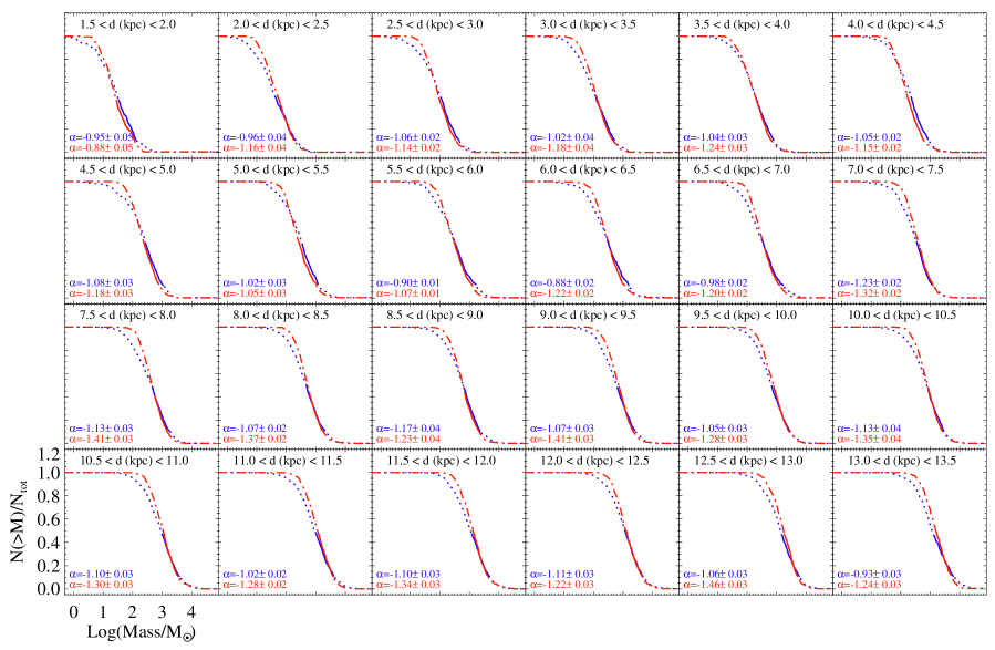
Figure 10: CClumpMFs for pre-stellar (red dotted-dashed line) and proto-stellar (blue dotted line), obtained in the same distance ranges used for Figure 9. The power-law (linear in bi-logarithmic scale) portion is highlighted with solid lines, and the corresponding slope is reported in the panel with the same colour coding.

In each panel of Figure 9 the peak of the ClumpMF and the completeness limit are shown for both pre- and proto-stellar distributions, while in Figure 10 the corresponding CClumpMFs are shown. The slopes obtained through the power-law fit range from -0.88 to -1.46 for the pre-stellar sources and from -0.88 to -1.23 for the proto-stellar ones. As expected from the discussion above, slopes of proto-stellar ClumpMFs are systematically shallower than the pre-stellar ones (cf. also di Francesco et al., 2010), being the former strongly biased by the lack of clumps at the highest mass bins compared with proto-stellar ones. In some cases, slopes of pre-stellar ClumpMFs can take values even steeper than the stellar Initial Mass Function (IMF, $\alpha_{\mathrm{IMF}}=-1.35$ Salpeter, 1955), as testified also by Tackenberg et al. (2012). On the contrary, the slopes of proto-stellar ClumpMFs remain always shallower than $\alpha_{\mathrm{IMF}}$, thus confirming the typical expectation for a generic mass distribution of unresolved clumps (Ragan et al., 2009; di Francesco et al., 2010; Peretto & Fuller, 2010; Eden et al., 2012; Pekruhl et al., 2013), while for the CoreMF a slope compatible with $\alpha_{\mathrm{IMF}}$ is typically found (e.g., Giannini et al., 2012; Polychroni et al., 2013; Könyves et al., 2015). On the one hand, this confirms, across a wide range of heliocentric distances and based on unprecedentedly large statistics, a behaviour of the ClumpMF already known from literature. On the other hand we caution the reader that $i$) the behaviour of the pre-stellar ClumpMFs has to be better investigated in the future (for example by means of higher-resolution observations of high-density pre-stellar cores, as suggested by Figure 8), and $ii$) the ClumpMFs discussed here are obtained regardless Galactic longitude, but simply grouping sources by heliocentric distance. More focused studies on selected ranges of Galactic longitude will enable the generation of mass distributions for even more coherent data sets, while also making it possible to explore environmental variations when looking at, e.g., individual spiral arms, tangent points, and star forming complexes. This, in turn, will allow assessment of similarities and differences among different Galactic locations.

Finally, ClumpMF slopes at different distances allow us to test the possible effects of gradual lack of spatial resolution on the ClumpMF slope. This problem has been already investigated by Reid et al. (2010) by means of simulations. Despite a depletion of sources in low-mass bins is expected at increasing heliocentric distance, together with an increase in high-mass bins due to blending, Reid et al. (2010) did not find a progressive shallowing of the ClumpMF. Here we can confirm, based on observational arguments, that the slopes reported across various panels of Figure 10 do not show any particular trend with distance. Therefore, whereas a clear distinction is found between the mass spectrum of cores (typically resolved by Herschel if located at $d\lesssim 1$ kpc, Giannini et al., 2012; Baldeschi et al., 2017), and that of clumps, with the former being steeper than the latter, no further systematic steepening is found for clumps observed at increasing distances. This might be also regarded as an indirect evidence of the self-similarity of molecular clouds (Stutzki et al., 1998; Smith et al., 2008; Elia et al., 2014) over the investigated range of physical scales, which, in this case, is the range of the linear sizes of compact sources located between $d=1.5$ and 13.5 kpc.

6.5 Bolometric luminosity and temperature

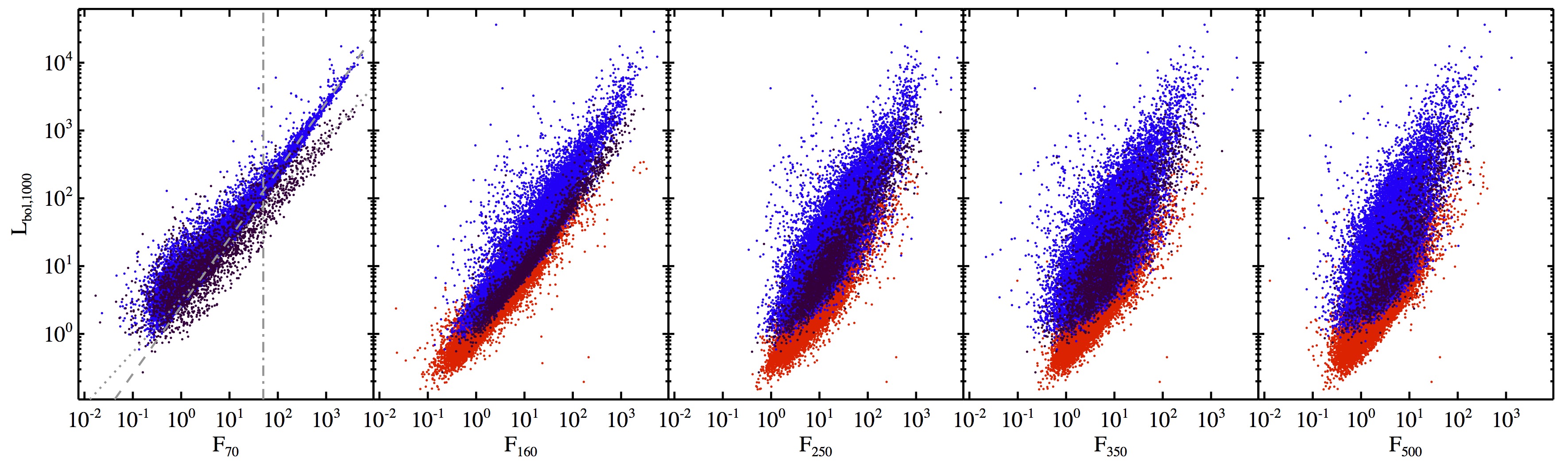
Figure 11: From left to right: source bolometric luminosity re-scaled to the virtual distance $d_{v}=1$ kpc vs Herschel monochromatic flux at 70, 160, 250, 350, and 500 $\mu$m, respectively. For clarity purposes, symbols of sources belonging to the same evolutionary class have been plotted all together: proto-stellar sources (blue) are overlaid on the pre-stellar sources (red), and MIR-dark proto-stellar sources (dark purple) are overlaid in turn on proto-stellar sources. In the leftmost panel (corresponding to the 70 $\mu$m case) the power-law fit is shown for sources with large fluxes ($F_{70}\gtrsim 50$ Jy, grey dotted-dashed vertical line), separately for the MIR-bright sub-sample (dashed line) and for the MIR-dark one (dotted-line).

Before discussing the use of bolometric luminosity, estimated as described in Section 4, to infer the evolutionary stage of a clump, we show how this quantity correlates with monochromatic Herschel fluxes. Indeed, Dunham et al. (2008) already suggested the Spitzer flux at 70 $\mu$m as a reliable proxy of the total proto-stellar core luminosity, and Ragan et al. (2012) confirmed an evident correlation between fluxes measured at all the three PACS bands (70, 100, and 160 $\mu$m) and bolometric luminosity of Herschel clumps. In the five panels of Figure 11 the bolometric luminosity, conveniently re-scaled to a common virtual distance $d_{v}=1$ kpc, is plotted vs the Herschel flux at different bands. The tightest correlation is found at PACS wavelengths, especially at 70 $\mu$m (left panel), where an overall power-law behaviour for MIR-bright sources can be identified at large fluxes ($F_{70}\gtrsim 50$ Jy). At lower fluxes one observes a departure of luminosity (observed also in Ragan et al., 2012) from the trend, which in this case represents the lower limit of the distribution. Interestingly, a secondary trend, similar to the main one but at a lower luminosity level and essentially due to MIR-dark proto-stellar sources, is observed $F_{70}\gtrsim 50$ Jy. The power-law best fit yields the expressions $L_{\mathrm{bol,MIR-bright}}[L_{\odot}]=2.56~{}F_{\mathrm{70}}[\mathrm{Jy}]^{1.00}$ (corresponding to linear behaviour, as in Ragan et al., 2012) and $L_{\mathrm{bol,MIR-dark}}[L_{\odot}]=3.29~{}F_{\mathrm{70}}[\mathrm{Jy}]^{0.79}$ for the two sub-samples in the considered range of fluxes, respectively.

The relation between bolometric luminosity and the envelope mass is particularly interesting as an indicator of the evolutionary status of a core/clump. The $L_{\mathrm{bol}}$ vs $M_{\mathrm{env}}$ diagram is a widely used tool (Saraceno et al., 1996; Molinari et al., 2008; André et al., 2008; Giannini et al., 2012; Ragan et al., 2013; Giannetti et al., 2013; Elia et al., 2013) in which evolutionary tracks, essentially composed by an accretion phase and a clean-up phase (Molinari et al., 2008; Smith, 2014), can be plotted and compared with data. In the earliest stages of star formation, as protostar gains mass from the surrounding envelope, these tracks are nearly vertical, while, after the central star has reached the Zero Age Main Sequence (ZAMS), they assume a nearly horizontal behaviour corresponding to dispersal of the residual clump material.

In Figure 12, left, we built the $L_{\mathrm{bol}}$ vs $M_{\mathrm{env}}$ plot using the bolometric luminosity obtained as described in Section 4, while the envelope mass is the source mass $M$ we derived through the grey body fit. For proto-stellar objects, $M_{\mathrm{env}}$ represents the residual mass of the parental clump/cloud still surrounding the embedded protostars, while for the starless sources it is the whole clump mass itself. Hereafter we will adopt $M_{\mathrm{env}}=M$. The right panel of the figure clarifies, by means of density contours, how proto-stellar sources are spread in a large area corresponding to a variety of ages, encompassing even evolutionary stages closer to the transition between clump collapse and envelope dissolution (ZAMS). However, since the bolometric luminosities are computed starting from the MIR ($\sim 20~{}\mu$m) or from longer wavelengths, while the most evolved Hi-GAL sources are expected to have also counterparts at shorter wavelengths (e.g., Li et al., 2012; Tapia et al., 2014; Strafella et al., 2015; Yun et al., 2015), it is likely that for a fraction of proto-stellar sources the evolutionary stage is underestimated, and the actual spread in age of this population is larger than represented here.

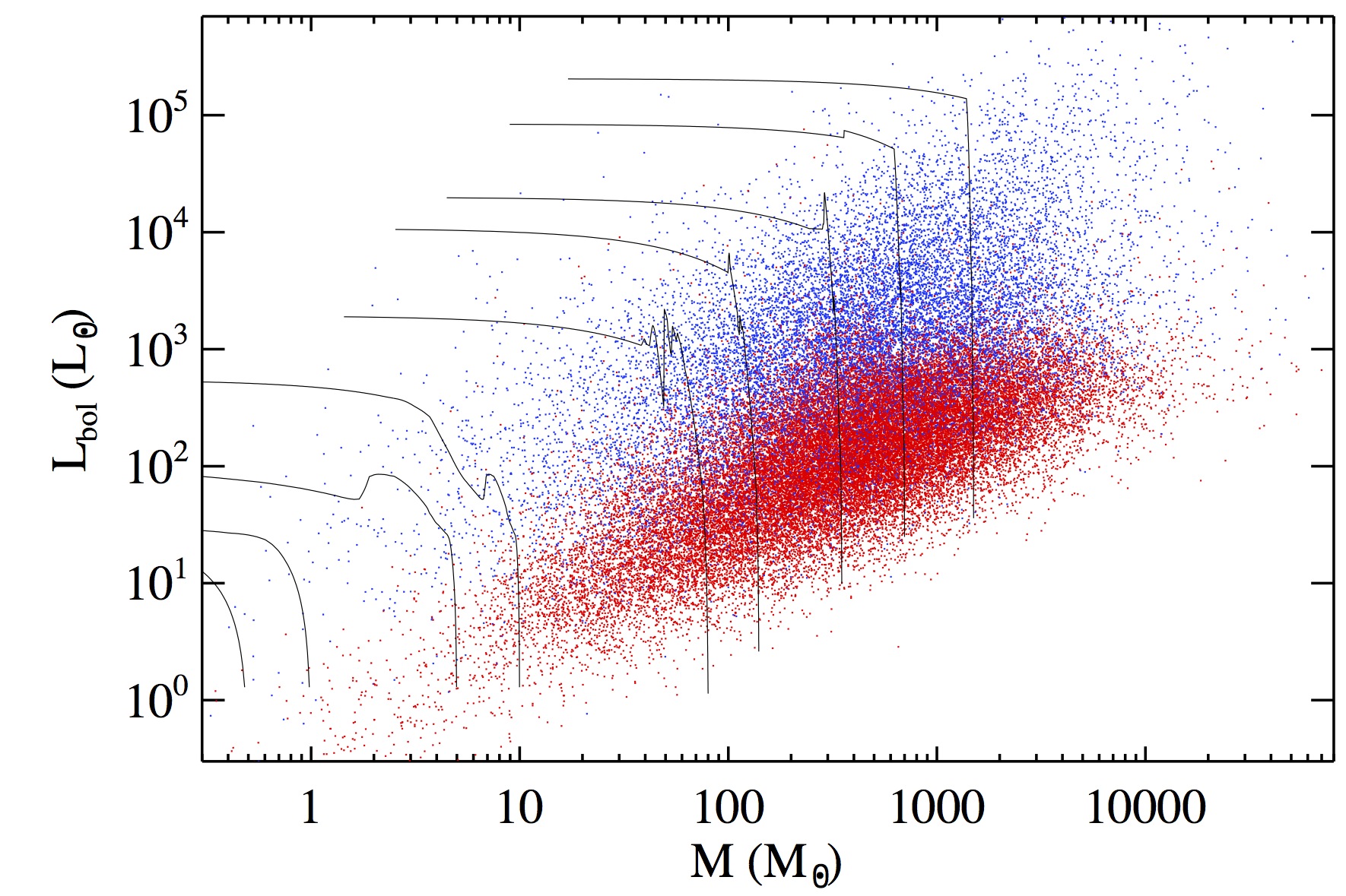
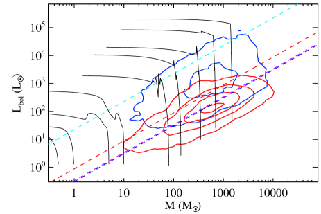
Figure 12: Left: $L_{\mathrm{bol}}$ vs $M_{\mathrm{env}}$ plot for all the sources considered in this paper. The black lines represent evolutionary tracks from Molinari et al. (2008). Right: The same as in the left panel, but with source density contours plotted instead of single sources. Contours are determined as in the bottom left panel of Figure 7, using levels of 5%, 25%, 50%, and 75% of the maximum density found in the plot. Dashed lines correspond to some relevant percentiles of the $L_{\mathrm{bol}}/M_{\mathrm{env}}$ ratio for different source populations (cf. Figure 13): in the area of the diagram below the red line, the 90% of pre-stellar sources are located, while above the blue, the dark purple and the light blue lines the 90% of all proto-stellar, MIR-dark proto-stellar and H ii-region-compatible sources are located, respectively.

As better highlighted by source density contours displayed in the right panel of Figure 12, pre-stellar sources are generally confined in a relatively narrower region corresponding to absence of collapse, or to the earliest clump collapse phases. This result can be compared with recent Hi-GAL works focused on smaller portions of the Galactic plane. In Veneziani et al. (2017), the clump populations at the tips of the Galactic bar, extracted from the entire catalogue presented here, show a similar behaviour. On the contrary, a comparison with the analysis of a portion of the third Galactic quadrant of Elia et al. (2013), as well as the larger number of sources considered and the spread over heliocentric distances (resulting in a wider range of masses and luminosities), highlights two points. First, the barycentre of the mass distribution is located towards higher values as a consequence of larger source distances involved in our sample. Second, a higher degree of overlap is seen between the pre- and proto-stellar source populationsthe former being found, at $M>10~{}M_{\odot}$, to be overlapped with the accretion portion of the evolutionary tracks, also populated by the proto-stellar sources. This does not mean necessarily that in the outer Galaxy a clearer segregation of the pre- vs proto-stellar clump populations is seen through this diagnostic tool (see also Giannini et al., 2012, for another example of analysis of an outer Galaxy region, namely Vela-C), since distance effects must also be taken into account. On average, the sources of Giannini et al. (2012) and Elia et al. (2013) are much closer ($d=700$ pc and $d\lesssim 2200$ pc, respectively) than most sources of our sample, and larger distances might introduce ambiguities in the pre- vs proto-stellar classification (see Appendix C). Further extension of the clump property analysis to other regions of the outer Galaxy (Merello et al., in prep.), and a systematic treatment of possible biases introduced by distance (Baldeschi et al., 2017) will make it possible to confirm this interpretation.

To express the relation between $L_{\mathrm{bol}}$ and $M$ through a single indicator one can use their ratio $L_{\mathrm{bol}}/M$ (cf., e.g., Ma et al., 2013; Molinari et al., 2016b), which has the advantage of being a distance-independent observable, allowing the use of the evolutionary analysis for catalogue entries devoid of a distance estimate. Figure 13 shows the histograms of this quantity for pre- and proto-stellar Hi-GAL sources, separately. Also here it can be seen that the distributions of $L_{\mathrm{bol}}/M$ ratios for pre-stellar and proto-stellar sources appear very different: in general, pre-stellar objects show a more confined distribution around 0.3 $L_{\odot}/M_{\odot}$, while proto-stellar sources are widely distributed with a peak around 2.5 $L_{\odot}/M_{\odot}$. A significant overlap of the two histograms is found in any case: notice, for instance, that 90% of pre-stellar sources are found at $L_{\mathrm{bol}}/M<0.9~{}L_{\odot}/M_{\odot}$, while 90% of proto-stellar sources are found at $L_{\mathrm{bol}}/M>0.3~{}L_{\odot}/M_{\odot}$ (Figure 12, right).

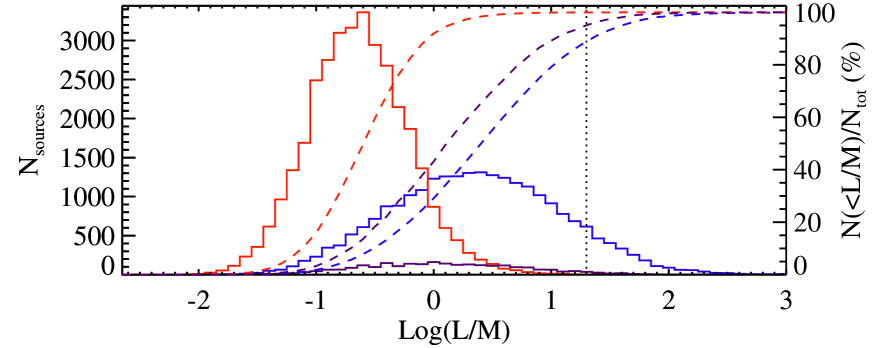
Figure 13: The same as in Figure 5, but for the $L_{\mathrm{bol}}/M$ ratio. The vertical dotted line represents the peak of the distribution of Cesaroni et al. (2015) (see text).

The larger width of the proto-stellar source distribution suggests that they are transition objects in an evolutionary phase between pure (yet starless) collapse and “naked” young stars without a dust envelope: the protostar(s) responsible for the increase in bolometric luminosity can be still embedded in a large cold dust envelope, responsible for keeping the mass of the entire proto-stellar clump high enough to reduce the $L_{\mathrm{bol}}/M$ ratio. Furthermore, one should keep in mind that conditions favourable to the formation of stars might be met only in a fraction of the entire volume of a distant proto-stellar clump. The observed $L_{\mathrm{bol}}/M$ ratio of a proto-stellar object is a single observable computed from the global emission of an envelope containing unresolved young stellar objects (YSOs) not necessarily coeval, but more generally at mixed stages of evolution (Yun et al., 2015).

From the analysis of the dust temperature distribution (Section 6.2) we could infer that MIR-dark proto-stellar sources are at an intermediate evolutionary stage between pre-stellar and MIR-bright proto-stellar sources. However, the $L_{\mathrm{bol}}/M$ metric indicates (see Figure 13) that this population spans a wide range of values, instead of being confined to the tail of the overall proto-stellar distribution. The cumulative distribution is only slightly different from that of the overall proto-stellar sample, and very different from that of the pre-stellar sample. Furthermore, the 10% percentile of this distribution (Figure 12, right panel) is indistinguishable from the same percentile computed for the proto-stellar population. In summary, the $L_{\mathrm{bol}}/M$ ratio for MIR-dark proto-stellar sources is not significantly different from that of the other proto-stellar sources.

To identify possible additional sub-classes within the proto-stellar population, the correlation with external evolutionary tracers can be used (as we intend to do in future papers based on this catalogue). For example, in the RMS survey (Lumsden et al., 2013) an effort has been made to identify massive YSOs and ultra-compact H ii regions by means of multi-wavelength ancillary data, both photometric and spectroscopic (e.g. Urquhart et al., 2009, and references therein). Similarly, for Hi-GAL Cesaroni et al. (2015) studied, in the longitude range $10^{\circ}<\ell<65^{\circ}$, the counterparts of CORNISH (Hoare et al., 2012; Purcell et al., 2013) sources, treated as bona-fide young H ii regions, and distributed across the range $2~{}L_{\odot}/M_{\odot}<L_{\mathrm{bol}}/M<270~{}L_{\odot}/M_{\odot}$. From the data of Cesaroni et al. (2015) we estimate the peak of this distribution to lie around $(L/M)_{\mathrm{P}}\equiv 22.4~{}L_{\odot}/M_{\odot}$. At values larger than this peak, in principle, even more evolved sources are expected, so the fact that the distribution decreases beyond this peak is mostly due to completeness: indeed the SED filtering we apply, mostly based on availability of detections at 250 and 350 $\mu$m, causes the removal of a large number of evolved sources from our physical catalogue.

The locus corresponding to $(L/M)_{\mathrm{P}}$ is reported also in Figure 12, right panel, as a light blue dashed line: if we compare it with a similar diagram in Molinari et al. (2008), we notice that their “IR sources”, namely the SEDs fitted with an embedded ZAMS envelope (many of which compatible with the presence of an ultra-compact H ii region), lie in the region of the diagram above this threshold.

Since our catalogue covers an area of the sky larger than that observed by the CORNISH survey to date, it would be useful to develop a Herschel-based method - verified by means of independent tracers - able to identify possible H ii-region candidates in other parts of the Galactic plane, such as the the fourth quadrant. For this reason the sources with $L_{\mathrm{bol}}/M\geq(L/M)_{\mathrm{P}}$ will henceforth be treated as “H ii-region candidates”.

Additional information can be obtained from the study of the source luminosity. For example, the $L_{\mathrm{smm}}/L_{\mathrm{bol}}$ ratio is a distance-independent evolutionary indicator frequently discussed in the study of the low-mass star formation. André et al. (2000) characterised Class 0 objects (Andre et al., 1993) through the ratio of their sub-millimeter luminosity, calculated for $\lambda\geq 350\mu$m, and their bolometric luminosity, establishing a minimum threshold of 0.005 for identifying an object of this class. Subsequently, Maury et al. (2011) refined this value to 0.01, which, if one prefers to use the inverse of this ratio (as, e.g., Beuther et al., 2010, and in this paper), translates into the condition $L_{\mathrm{bol}}/L_{\mathrm{smm}}<100$. Obviously, the Class 0/I/II/III is meaningful only for single low-mass protostars, while in our study we address sources which do not correspond to single YSOs and, furthermore, in a relevant fraction of cases these might host massive star formation. Therefore in our case the $L_{\mathrm{bol}}/L_{\mathrm{smm}}$ ratio cannot be used to identify Class 0 sources (see also Fallscheer et al., 2013), rather we can only safely state that sources whose SEDs have a significant contribution of emission at sub-millimetric wavelengths are at an early stage of star formation.

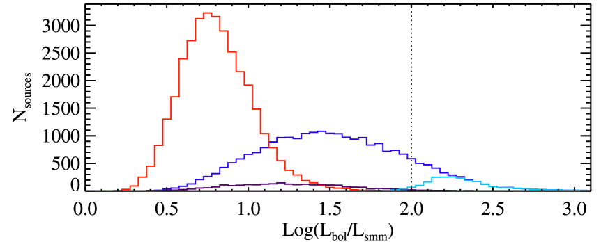
Figure 14: Distributions of $L_{\mathrm{bol}}/L_{\mathrm{smm}}$ ratio for science analysis in this paper: pre- and proto-stellar ones are represented with a red and blue histogram, while the MIR-dark and H ii-region candidate sub-samples of the proto-stellar ones are represented with a dark purple and a light blue histogram, respectively. The dotted vertical line represents the threshold for identifying Class 0 YSO in the low-mass regime of star formation (Maury et al., 2011).

In Figure 14 the distributions of $L_{\mathrm{bol}}/L_{\mathrm{smm}}$ for pre- and proto-stellar sources are shown, again exhibiting a different behaviour of the two: the former (having about 99.96% of sources below the critical value of 100) peaks at a value smaller than the latter, which, in turn, has only 86% below the threshold. Since many of the sources of our catalogue belong to well-known star forming regions where the presence of sources more evolved than Class 0 has been assessed, these results clearly indicate that an evolutionary classification based only on Herschel photometry (even extended to shorter wavelengths down to $\sim 20~{}\mu$m), generally leads to a biased classification of most sources as Class 0 (or, more precisely, as their high-mass equivalents), as already pointed out by Giannini et al. (2012) and Elia et al. (2013). Looking in more detail at the two sub-classes of proto-stellar sources introduced above, the MIR-dark sources how a spread similar to that encountered in Figure 13, while the H ii-region candidates constitute the right tail of the proto-stellar distribution, with most bins located above the threshold value of 100.

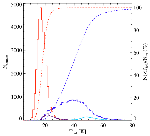
Figure 15: The same as in Figure 5, but for the bolometric temperature.

An even higher degree of segregation between pre- and proto-stellar sources can be found in the bolometric temperature distribution shown in Figure 15, being defined by Myers & Ladd (1993) as:

$$T_{\mathrm{bol}}=1.25\times 10^{-11}~{}\mathrm{K}\times\frac{\int_{0}^{\infty}\nu~{}F_{\nu}~{}d\nu}{\int_{0}^{\infty}~{}F_{\nu}~{}d\nu}\;.$$ (5)

This diagnostic has been used recently by Strafella et al. (2015) by using Hi-GAL data, but building SEDs with a wider range of photometric data points, going from Spitzer-IRAC bands, which can lead to a shift of bolometric temperatures towards values as $T_{\mathrm{bol}}\sim 100-1000$ K, much larger than those found here ($T_{\mathrm{bol}}\lesssim 100$ K). In fact, similarly to the $L_{\mathrm{smm}}/L_{\mathrm{bol}}$ ratio, bolometric temperatures cannot be used to infer the Class 0/I/II/III source classification (Lada & Wilking, 1984; Lada, 1987; Andre et al., 1993), according to which almost all sources of our catalogue would fall in the Class 0 range ($T_{\mathrm{bol}}<70$ K, Chen et al., 1995). At the same time, by revealing a net separation between pre- and proto-stellar clumps and a pronounced spread inside the distribution of the latter, bolometric temperatures can still be used to highlight the variety in evolutionary stage of the Hi-GAL sources.

Looking at the histogram of the MIR-dark proto-stellar sources in Figure 15, it is evident that these sources represent the low-$T_{\mathrm{bol}}$ tail of the overall proto-stellar distribution. This is expected, given the $T_{\mathrm{bol}}$ definition (see Equation 5), since small MIR fluxes correspond to low $T_{\mathrm{bol}}$ values. On the contrary, the H ii-region candidates are located towards the highest probed bolometric temperatures, although they do not constitute the totality of proto-stellar sources at these temperatures. This suggests that bolometric temperature and $L_{\mathrm{bol}}/M$ are not perfectly coupled, as it will be discussed in Section 7.2.

In general, typical bolometric temperatures are found to range from $\sim 10$ K (pre-stellar sources) to $\sim 80$ K, a range incompatible with average values for the clump populations of Mueller et al. (2002), 78 K, and Ma et al. (2013), 113 K. A direct comparison with these two works, however, is not appropriate due to the different spectral ranges covered, with the MIR range dominated, in those cases, by IRAS fluxes (see Appendix D for a more detailed comparison between the clump properties derived by Ma et al., 2013, and those in the present work).

7 An evolutionary scenario

In this section we synthesize the physical quantities described above with the aim to formulate an evolutionary classification scheme for proto-stellar sources.

7.1 Herschel colours

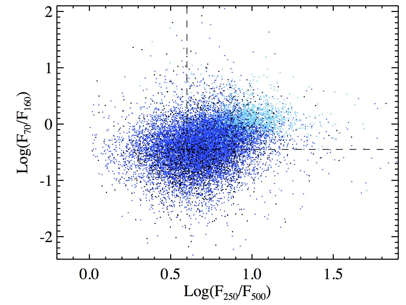
Figure 16: Plot of the $F_{70}/F_{160}$ vs $F_{250}/F_{500}$ colours for the sub-sample of proto-stellar sources (blue dots) provided with fluxes at these four bands. The positions of sources with no detection in the MIR are overplotted as black dots, while sources identified as H ii regions (see the text), are overplotted as light blue dots. The dashed lines delimit the area identified by Paladini et al. (2012) to contain H ii regions.

Examples of Herschel-based colour-colour diagrams are found in literature as tools to perform source evolutionary classification. While here we can not apply the prescriptions such as those given in Ali et al. (2010) or Spezzi et al. (2013), intended for classifying single low-mass YSOs in nearby star forming regions, it is however interesting to consider and extend the analysis of Paladini et al. (2012) of a sample of 16 H ii regions observed in Hi-GAL around $\ell=30^{\circ}$. In Figure 16, following these authors, we build the $F_{70}/F_{160}$ vs $F_{250}/F_{500}$ diagram for the proto-stellar sources of our sample with fluxes at these four wavelengths. Paladini et al. (2012) identify a region at the top-right of the diagram, in which Herschel fluxes of analysed H ii regions are found to lie (despite some contamination by non H ii regions). We find that 8034 of the considered sources (i.e. 48% of the total) are located in this area of the diagram. We highlight with a different colour the positions of sources fulfilling the condition $L_{\mathrm{bol}}/M\geq(L/M)_{\mathrm{P}}$, that we assume to be H ii region candidates. We find that the great majority of such sources (1297 out of 1391, i.e. the 93%) lie well inside the region defined by Paladini et al. (2012).

It is interesting to explore also the behaviour of the sub-sample of proto-stellar MIR-dark sources, which are expected to correspond to an earlier evolutionary phase. These appear not to be confined to the H ii-region locus and are generally more spread out. This indicates that this choice of Herschel colours does not appear to be correlated with the presence of one or more MSX/WISE/Spitzer counterparts.

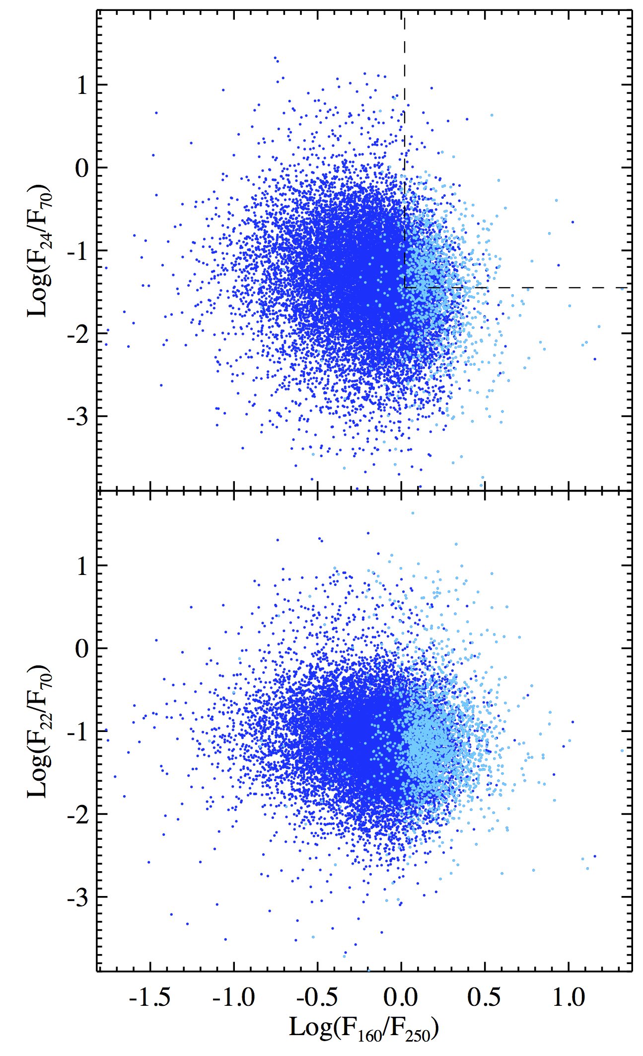
Figure 17: The same as Figure 16, but for the colours $F_{24}/F_{70}$ (top) and $F_{22}/F_{70}$ (bottom) vs $F_{70}/F_{160}$. Each of the two plots is based on the sub-sample of proto-stellar sources provided with the four fluxes requested to build it. In the top panel, the dashed lines delimit the area occupied by H ii regions in the analogous colour-colour diagram of Paladini et al. (2012).

Another diagnostic used by Paladini et al. (2012) is $F_{24}/F_{70}$ vs $F_{160}/F_{250}$ diagram, thus involving the Spitzer-MIPS flux at $24~{}\mu$m, which is shown in Figure 17, top panel. As sources with $F_{24}\gtrsim 2$ Jy tend to be saturated in MIPS (Carey et al., 2008), we also construct a $F_{22}/F_{70}$ vs $F_{160}/F_{250}$ diagram using WISE $22~{}\mu$m data (Figure 17, bottom panel). In both panels, data appear highly scattered, though the sub-sample of sources identified as H ii-region candidates still occupy a smaller area of this space, where Log$(F_{160}/F_{250})>0$, similarly to Paladini et al. (2012). The large scatter in the $y$ direction, however, demonstrates that a MIR counterpart does not provide leverage to separate out early-stage sources from a more evolved population in these diagrams.

7.2 Bolometric quantities

Here we explore the relations between the parameters and attempt to use these to better define the evolutionary sequence of proto-stellar sources.

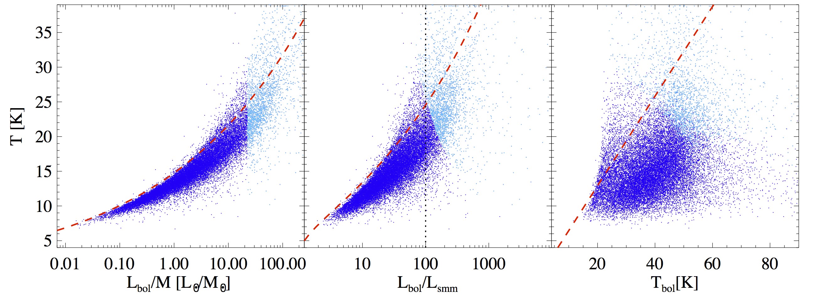
Figure 18: Plot of temperature $T$ of proto-stellar sources (blue dots) vs the $L_{\mathrm{bol}}/M$ ratio (left), the $L_{\mathrm{smm}}/L_{\mathrm{bol}}$ ratio (centre), and the bolometric temperature $T_{\mathrm{bol}}$ (right), respectively. The sub-sample of sources compatible with a H ii region is plotted in cyan. Red dashed lines represent, in each panel, the expected behaviour of an optically thin grey body (Equation 4) with $\beta=2$, as derived by Elia & Pezzuto (2016). In the centre panel, the vertical dotted line is the same as in Figure 14.

In Section 6.2 a mild segregation between pre- and proto-stellar clump grey-body temperatures was found. In Figure 18, we directly compare the dust temperature with evolutionary indicators such as $L_{\mathrm{bol}}/M$, $L_{\mathrm{bol}}/L_{\mathrm{smm}}$, and $T_{\mathrm{bol}}$, introduced in Section 6.5. As expected, all three quantities increase as a function of $T$. Also, at a given temperature most of proto-stellar clumps show an excess of these quantities with respect to the theoretical behaviour of a grey body with $\beta=2$.

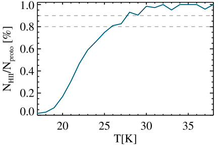
Figure 19: Fraction of proto-stellar sources classified as H ii-region candidates ($L_{\mathrm{bol}}/M\geq(L/M)_{\mathrm{P}}$) over the total number of the proto-stellar ones vs temperature. The two horizontal dashed lines indicate the 80% and 90% levels.

Two general considerations emerge from the three panels of this figure: since the average temperature estimated for proto-stellar sources is dominated by the cold envelope modelled as a grey body, it subtends a certain degree of degeneracy of evolutionary stages, which can be resolved thanks to indicators (reported on the $x$-axes of the three panels), which are derived by including emission at wavelengths shorter than $70~{}\mu$m. On the other hand, at the behaviour of some of the more evolved sources in our sample, such as those compatible with a H ii region based on their $L_{\mathrm{bol}}/M$ (see Section 6.5), their temperature is definitely high. In Figure 19, the fraction of proto-stellar sources classified as H ii-region candidates out of the total number of proto-stellar sources per bins of temperature is shown: at $T\gtrsim 26$ K, 80% of the proto-stellar sources have a $L_{\mathrm{bol}}/M$ greater than the threshold required for classifying it as a H ii-region candidate, while 90% level is achieved at $T\gtrsim 28$ K. This is in good agreement with the estimate of $T=25$ K by Hofner et al. (2000) for clumps hosting ultra-compact H ii regions.

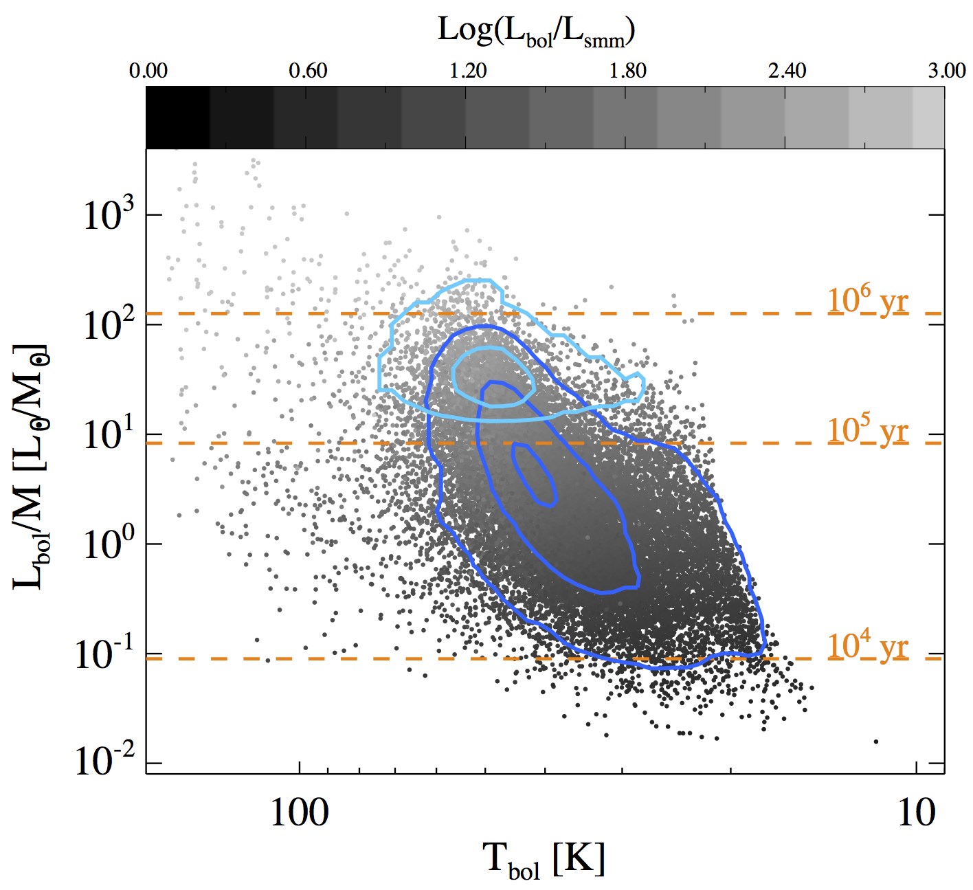
Figure 20: Plot of $L_{\mathrm{bol}}/M$ vs $T_{\mathrm{bol}}$ for proto-stellar sources. The dot colour depends on the $L_{\mathrm{smm}}/L_{\mathrm{bol}}$ ratio of the source, ranging logarithmically from 1 to 1000 (from the darkest to the lightest level of grey present in the plot, respectively; for values outside this range the colour scale saturates). Blue and light blue contours represent the areas enclosing, from the innermost to the outermost contour, the 10%, 50%, and 90% of all the proto-stellar sources, and of the H ii-region candidates, respectively. Dashed orange lines correspond to $L_{\mathrm{bol}}/M$ achieved after $10^{4}$, $10^{5}$, and $10^{6}$ yr along the rightmost evolutionary track of Figure 12.

To show more directly the mutual connections among $L_{\mathrm{bol}}/M$, $L_{\mathrm{bol}}/L_{\mathrm{smm}}$, and $T_{\mathrm{bol}}$, in Figure 20 we plot $L_{\mathrm{bol}}/M$ vs $T_{\mathrm{bol}}$ for proto-stellar sources, while also showing $L_{\mathrm{bol}}/L_{\mathrm{smm}}$ by means of a colour scale. The source density contours, both for the entire sample of proto-stellar sources and for the H ii-region candidates, guide the reader through the most crowded areas of the plot.

The evolutionary tracks of Molinari et al. (2008), reported in Figure 12, can be used for providing a rough estimate of the time elapsed since the beginning of the collapse given a value of the $L_{\mathrm{bol}}/M$ ratio. In Figure 20 $L_{\mathrm{bol}}/M$ values of $10^{4}$, $10^{5}$, and $10^{6}$ yr corresponding to the highest mass track, i.e. the one starting at an initial mass $M_{0}=1500~{}M_{\odot}$, are displayed as horizontal lines. According to this rough timescale, the figure suggests that a large fraction of proto-stellar sources ($18482$ objects) would correspond to an age of $t<10^{5}$ yr, while H ii-region candidates are found to be well above that value. Comparing with proto-stellar (Class 0 + I) phase lifetimes of a few $10^{5}$ yr quoted by Dunham et al. (2014) for cores in the Gould Belt, we find that the majority of proto-stellar sources present in Figure 20 correspond to a shorter evolutionary time: this indicates a faster evolution for clumps hosting formation of more massive stars, as a significant part of Hi-GAL clumps are generally supposed to be (cf. Section 6.3).

Recently (Molinari et al., 2016b) calibrated the $L_{\mathrm{bol}}/M$ through CH₃C₂H(12-11) line observations, finding that $i$) this line is detected at $L_{\mathrm{bol}}/M>1L_{\odot}/M_{\odot}$ (which should correspond to a temperature $T<30$ K in the inner part of the clump), and $ii$) the temperature indicated by this tracer starts to increase at $L_{\mathrm{bol}}/M>10L_{\odot}/M_{\odot}$, where this threshold is interpreted as the first appearance of ZAMS star(s) in the clump. Comparing this scenario with our statistics, we find that 50% of our proto-stellar clumps have $L_{\mathrm{bol}}/M$ between 1 and 10 $L_{\odot}/M_{\odot}$, with an average bolometric temperature of 40 K. Only 20% of proto-stellar clumps, however, have $L_{\mathrm{bol}}/M>10L_{\odot}/M_{\odot}$, while - as we expect (since $(L/M)_{\mathrm{P}}>10L_{\odot}/M_{\odot}$) - all of the H ii-region candidates, are above this threshold, having an average bolometric temperature of 55 K.

The $L_{\mathrm{bol}}$ vs $T_{\mathrm{bol}}$ is a diagnostic used to characterise the YSOs from the evolutionary point of view (Myers et al., 1998). Recently, Strafella et al. (2015) applied it to a population of Hi-GAL sources all belonging to the same region (Vela-D), assumed to be located at the same heliocentric distance. On the one hand, it is possible to remove the dependence on distance by taking into account $L_{\mathrm{bol}}/M$ instead of $L_{\mathrm{bol}}$. The $L_{\mathrm{bol}}/M$ vs $T_{\mathrm{bol}}$ source behaviour in Figure 20 is qualitatively similar to Figure 9 of Strafella et al. (2015), given the strongly different amount of sources and the different quantity reported on the $y$-axis, as explained above. A similar range of $T_{\mathrm{bol}}$ is found, as well as some spread in $L_{\mathrm{bol}}/M$. This spread becomes remarkably large at high $T_{\mathrm{bol}}$, highlighting that these two indicators can, in a few cases mostly concentrated at high bolometric temperatures, give conflicting information about the evolutionary stage of a source.

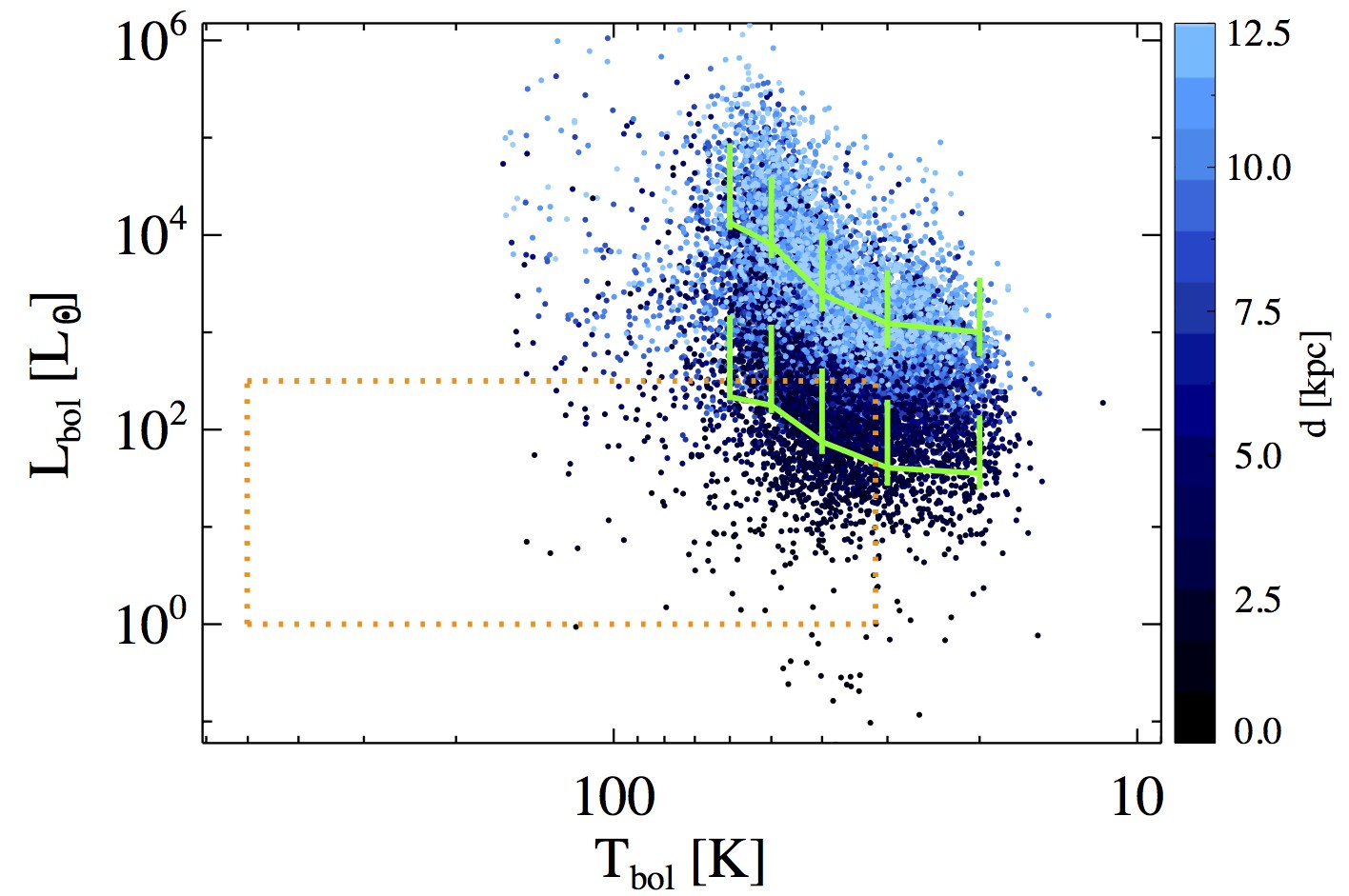
Figure 21: Plot of $L_{\mathrm{bol}}$ vs $T_{\mathrm{bol}}$ for proto-stellar sources. The dot colour, described by the colour bar on the right, scales with the source heliocentric distance (the scale saturates at 12.5 kpc). The orange dashed box corresponds to the region occupied in this diagram by the Herschel+Spitzer proto-stellar sources studied in Vela-C by Strafella et al. (2015). As an example, median values of the luminosity calculated over six bins of $T_{\mathrm{bol}}$ (starting from 20 K and in steps of 10 K) for sources at $d>10$ kpc (upper green broken line) and at $d<3$ kpc (lower green broken line), respectively, are shown. The typical distribution of luminosities being strongly skewed, with a longer tail at high luminosities, it does not make sense to show, as error bars, the values of the standard deviation; therefore here we use bars defined by the 15th (bottom of the bar) and the 85th percentile (top), enclosing 70% of luminosity values present in the considered bin of $T_{\mathrm{bol}}$.

On the other hand, a direct comparison with the plot of Strafella et al. (2015) can be performed binning sources with respect to distance, which is rendered in Figure 21 through a colour scale. The box enclosing the positions of the proto-stellar cores in the analogous plot reported in that paper ($30$ K $\lesssim T_{\mathrm{bol}}\lesssim 500$ K, $1~{}L_{\odot}~{}\lesssim L_{\mathrm{bol}}\lesssim 300~{}L_{\odot}$) still contains a relevant number of sources (2470) from our sample. Nevertheless, a significant fraction of the sources of Strafella et al. (2015) are found to have $T_{\mathrm{bol}}>100$ K, while most of our sources lie below that value. This is essentially due to the wider wavelength range considered by these authors to compute $T_{\mathrm{bol}}$, starting from $3.6~{}\mu$m, which inevitably leads $T_{\mathrm{bol}}$ to increase according to Equation 5.

Grouping sources with comparable distances, a general trend of the luminosity to strongly increase at increasing bolometric temperature is seen in the range $15~{}$K $\lesssim T_{\mathrm{bol}}\lesssim 65$ K in which sample is large enough to reconstruct such a behaviour. This can be seen through two examples we give in Figure 21, considering sources in the two very different distance ranges, namely $d<3$ kpc and $d<10$ kpc. However, in such examples, the log-log slope of $L_{\mathrm{bol}}$ vs $T_{\mathrm{bol}}$ is everywhere shallower than 6, which is the value expected for a perfect grey body with $\beta=2$ (cf. Equations 35 and 44 of Elia & Pezzuto, 2016). This means that, although the departure from a cold grey body behaviour observed in proto-stellar envelopes at $\lambda<160~{}\mu$m introduces an excess both in $L_{\mathrm{bol}}$ and $T_{\mathrm{bol}}$, the latter is more sensitive than the former to the extension of the SED towards shorter wavelengths. Notice that this qualitative consideration is given neglecting the further effect of the spread in distance underlying the two samples used to draw the curves in Figure 21.

7.3 Surface density

Here we search for possible correlations between the main source evolutionary indicators and the source surface density introduced in Section 6.3. Notice that this parameter is not derived from only photometric measurements, but also from the source linear size.

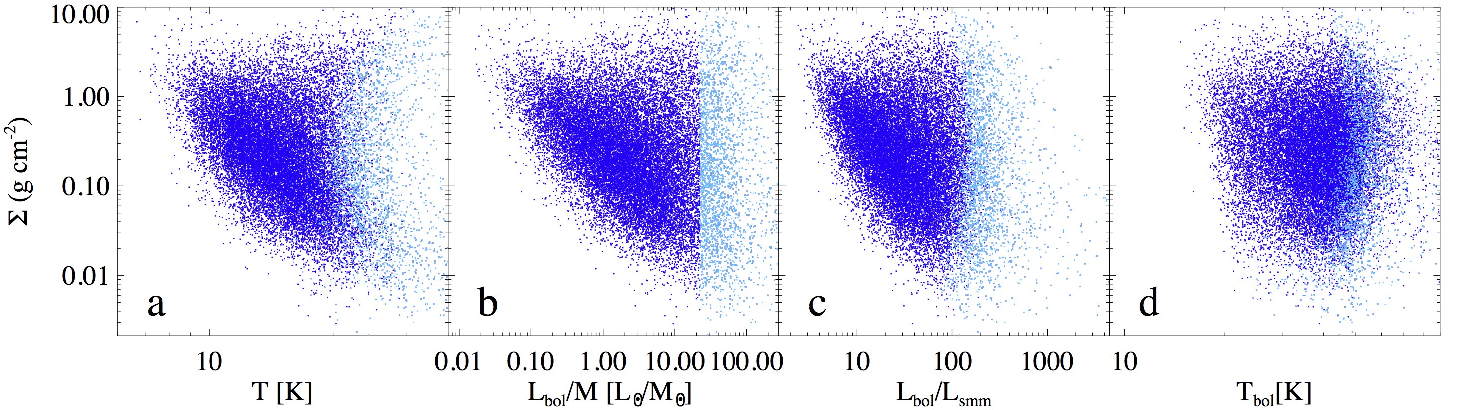
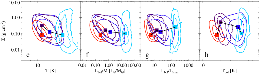
Figure 22: Upper panels: relation between clump surface density and, from panel a to d, dust temperature, $L_{\mathrm{bol}}/M$, $L_{\mathrm{bol}}/L_{\mathrm{smm}}$, and bolometric temperature, respectively. Blue dots represent proto-stellar clumps, except for the sub-sample of sources compatible with a H ii region, plotted in cyan. Lower panels (e-h): the same diagrams as in the upper panels, but with source density contours enclosing the 90% and the 20% of sources, respectively. Contours describing the sample of pre-stellar sources and the sub-sample of MIR-dark proto-stellar sources are also plotted in red and dark purple, respectively. In absolute terms, hence, the contours drawn for different populations correspond to different values: for example, 34021 being the total number of pre-stellar sources considered for building this plot, the external contour is drawn in order to contain 6804 sources, and the internal one to contain 30618 sources; the total numbers of proto-stellar, candidate H ii regions, and MIR-dark sources are 24397, 2377, and 2535, respectively (notice that the second and third population are sub-samples of the first one), from which the values corresponding to the source density contours can be easily derived as in the example above. Finally, in each panel the peaks of the source distributions of the four aforementioned evolutionary classes are reported with filled circles of same colours of the contours, and connected by a black line.

In Section 6.3 we have shown that proto-stellar sources are found to be, on average, slightly smaller and denser than starless ones (Figures 4 and 7). A the same time, clump column density is observed to decrease with increasing temperature (e.g. IRDCs, Peretto et al., 2010), in such a way that the combination of these two opposing effects contribute to the overlap between the surface density distributions of the starless and proto-stellar populations seen in Figure 7. In Figure 22, panel $a$, surface density vs dust temperature relation is plotted for proto-stellar sources. The bulk of sources show the aforementioned trend, but with increasing temperatures the spread in surface density increases, so that a remarkable fraction of sources which appear to be, at the same time, dense and warm is found: for instance, considering proto-stellar sources with $T>25$ K, 673 have $\Sigma\leq 0.1$ g cm² and 611 have $\Sigma>0.1$ g cm² (52% and 48% of the total, respectively). In particular, candidate H ii regions are found at the highest temperatures, but the position in the plot is not indicative of any particular trend, spanning the entire range of surface densities, from 0.01 to 10 g cm^-2.

Not surprisingly, a similar behaviour is found for $\Sigma$ vs the $L_{\mathrm{bol}}/M$ ratio (Figure 22, panel $b$), given the tight correlation between $T$ and $L_{\mathrm{bol}}/M$ seen in Figure 18. The plot in panel $c$ of $\Sigma$ vs $L_{\mathrm{bol}}/L_{\mathrm{smm}}$ is very similar to the previous one, as expected. Finally, a larger spread with respect to previous panels is found in the $\Sigma$ vs the $T_{\mathrm{bol}}$ plot. To highlight a possible evolutionary sequence emerging from these diagrams we report them in the bottom panels of Figure 22, showing the source density contours not only for the populations of in panels $a$-$d$, but also for pre-stellar and MIR-dark proto-stellar sources. The pre-stellar population occupies a relatively small region in the left part of the diagrams, while apparently no large differences are found between contours of MIR-dark and overall proto-stellar sources. This confirms the impression obtained in previous sections, namely that the MIR-dark sources do not necessarily constitute the “earliest-stage tail” of the proto-stellar population. Some degree of segregation is found only with respect to the bolometric temperature (panel $d$), as already suggested by Figure 15. Finally, the H ii region candidates occupy the right portion of all plots, showing the largest scatter in surface density. Despite the large scatter and partial overlap among different classes of objects, if we consider - in each plot - only the peaks of the source density contours, an evolutionary sequence through various classes might be identified: MIR-dark sources are typically denser than pre-stellar but also generic proto-stellar ones, and H ii region candidates are normally found at lower densities than the generic proto-stellar sources. On average proto-stellar sources are denser than the starless ones, and characterised by a wide range of densities, often showing a surface density increase in the early stages of star formation, followed by a drop with increasing age (corroborating the results of Giannetti et al., 2013; Guzmán et al., 2015), although cases of evolved sources with large surface densities are also found.

7.4 A tool for source classification

Having examined the clump physical parameters as evolutionary diagnostics, we show a “radar-plot” visualization of these, which allows a powerful and compact way to show multivariate data. In particular, we chose five distance-independent quantities, namely $T$, $L_{\mathrm{bol}}/M$, $L_{\mathrm{bol}}/L_{\mathrm{smm}}$, $T_{\mathrm{bol}}$, and $\Sigma$.

Figure 23: Radar plot for the median of five physical parameters (see text) for the classes of pre- and proto-stellar clumps (red and blue lines, respectively). Solid lines represent the statistics of the entire populations, whereas separate statistics for the fourth and the first Galactic quadrants (see Section 8.1) are represented with dashed and dotted lines, respectively. Scales on each axis are linear, ranging from 0 to the value specified at the end.

In Figure 23 the medians of the five indicators for the whole classes of pre- and proto-stellar clumps are reported on the five axes of the radar plot, and points are connected through a polygonal line to form a pentagon. One can notice that the pentagon corresponding to the proto-stellar sources includes the pentagon representing the pre-stellar ones, since the values of the considered age indicators are typically larger for the former class of objects. Such a behaviour is also estimated, independently, for the fourth and the first Galactic quadrant, as we will discuss in Section 8.1.

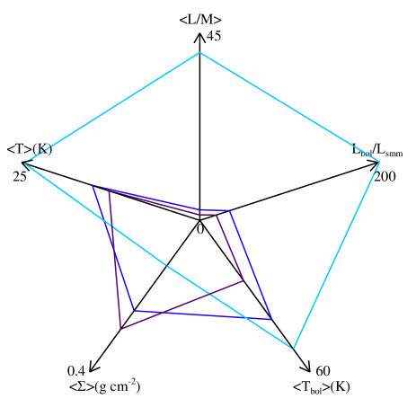
Figure 24: As in Figure 23, but for proto-stellar sources (blue line) and for the two extracted populations of MIR-dark sources (dark purple line) and H ii-region candidates (light blue line), respectively.

The radar plot of the proto-stellar sources can be further compared with that of the two sub-samples we discussed in previous sections as possible extremes of their age distribution: the MIR-dark and the candidate H ii regions, respectively. In Figure 24 all evolutionary indicators appear decreased for the MIR-dark sample, and enhanced for the candidate H ii regions, with respect to the overall proto-stellar population, except for the surface density which, as seen in Section 7.3, exhibits the opposite global trend.

The metric described above could be used in future, for instance, to characterise the properties of clump populations associated with IRDCs (e.g., Traficante et al., 2015), lying on (vs off) filaments (e.g., Schisano et al., 2014), located in the outer (vs inner) Galaxy, etc. Moreover, this representation of the median (or mean) properties of a sample can be applied to a single source, allowing one to to immediately assess if and how this approaches or deviates from the global behaviour of a certain class of sources it, in principle, belongs to.

8 Source spatial distribution along the Galactic Plane

8.1 First vs fourth Galactic quadrant

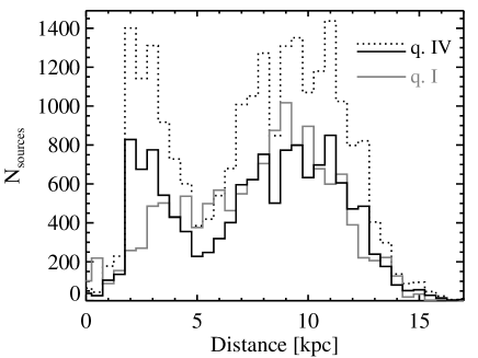
Figure 25: Source heliocentric distance distributions (cf. Figure 4, left), obtained separately for the fourth (black) and the first (grey) quadrant, respectively. To better compare the two distributions, the original fourth quadrant histogram (dotted line) has been normalized (solid line) by the ratio of the total source counts in the two quadrants.

So far we considered the global statistics of the Hi-GAL sources regardless of their position in the Galactic plane. In this section the statistics of Hi-GAL source properties is presented in bins of Galactic longitude, and discussed in view of a comparison between the fourth and first quadrant. To introduce this analysis, with particular respect to the discussion of distance-dependent observables, first of all we show the heliocentric distance distribution in the fourth and the first Galactic quadrants, separately (Figure 25). The main differences, i.e. those extending over more than two bins, are seen around 3-4 kpc, where fourth-quadrant sources are predominant in number, and around 4.5-7 kpc, where the opposite case is found. However, the overall behaviour of the two distributions is similar, thus making a comparison between the two quadrants feasible for distance-dependent properties such as mass, linear size and luminosity (see below).

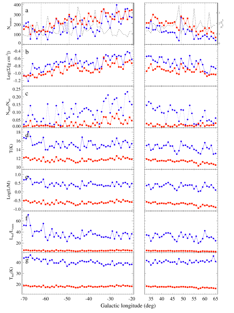
Figure 26: Distribution of relevant quantities obtained in this paper for pre- (red filled squares) and proto-stellar (blue filled circles) sources as a function of the Galactic longitude, averaged over bins of width $1^{\circ}$, in the longitude range of the fourth (left panels) and the first (right panels) Galactic quadrants considered in this work: ($a$) source number (where the where the dotted black line represents the pre- over proto-stellar source number ratio reported on the right axis); ($b$) median of decimal logarithm of surface density; ($c$) fractional number of dense clumps fulfilling conditions for massive star formation (according to Krumholz & McKee, 2008) ; ($d$) median temperature; ($e$) median of decimal logarithm of $L_{\mathrm{bol}}/M$; ($f$) median of the $L_{\mathrm{bol}}/L_{\mathrm{smm}}$ ratio; ($g$) median of bolometric temperature.

Figure 26 presents the starting points for discussing the distribution of sources and their properties in the plane. Panel $a$ shows how sources are distributed in longitude. A relation with the trends found in single-band catalogues by Molinari et al. (2016a) is expected despite the SED filtering carried out in this work. In fact, for each physical quantity we have considered, $i$) a positive correlation is found moving towards the inner Galaxy, and $ii$) as shown by Molinari et al. (2016a), for both pre- and proto-stellar sources localized excesses are found at positions corresponding to spiral arm tangent points or star forming complexes.

Enoch et al. (2008) used the number ratio between starless and proto-stellar cores to roughly estimate, through a proportionality factor, the lifetime of the cores they detected in nearby low-mass star forming regions. Because, in our case, we are dealing with clumps instead of cores, we cannot apply a similar prescription directly, although useful considerations can be made concerning clumps. Our clump statistics gives a ratio of $\sim 1$ which, as found by Svoboda et al. (2016) on their sample of 4683 clumps identified at 1.1 mm in the first quadrant, would be suggestive of comparable lifetimes for the two classes (see also Motte et al., 2010b; Ragan et al., 2013). Here, thanks to large statistics, we are able to describe this quantity, $N_{\mathrm{pre}}/N_{\mathrm{prt}}$ as a function of Galactic longitude (Figure 26, panel $a$). Pre-stellar sources are in excess with respect to proto-stellar ones almost everywhere, except for a few cases where $N_{\mathrm{pre}}/N_{\mathrm{prt}}<1$ in the fourth quadrant. In general, this ratio is lower in the fourth quadrant, i.e. 1.25 vs 1.63 for the first quadrant.

To infer relative clump lifetimes from this number ratio is not trivial, since time scales can also depend on the mass. Indeed the deficit of pre-stellar sources with respect to proto-stellar ones at both the lowest and the highest masses found at a given heliocentric distance was extensively discussed in Section 6.4, concluding that in particular, it should be due to rapid evolution of the most massive, but also densest pre-stellar clumps from the quiescent phase to star forming activity. A synoptic look at panels $a$ and $b$ (the latter showing the median surface density) of Figure 26 seems not to confirm such a scenario, since no evident correlation is seen between $N_{\mathrm{pre}}/N_{\mathrm{prt}}$ and density. However, plotting the former against the latter (Figure 27, top panel), values of $N_{\mathrm{pre}}/N_{\mathrm{prt}}>2$ are found only for lower median surface densities of pre-stellar sources ($\Sigma\lesssim 0.15$ g cm²). Furthermore, at higher densities ($\Sigma\gtrsim 0.2$ g cm²), only cases with $N_{\mathrm{pre}}/N_{\mathrm{prt}}<1.3$ are found. Unfortunately we can not consider this as a strong argument, since the inverse of these statements is not found to be true in general. Future studies, focused on a more accurate identification and analysis of specific regions characterised by a very high or a very low $N_{\mathrm{pre}}/N_{\mathrm{prt}}$, will better assess the relation with pre-stellar clump density.

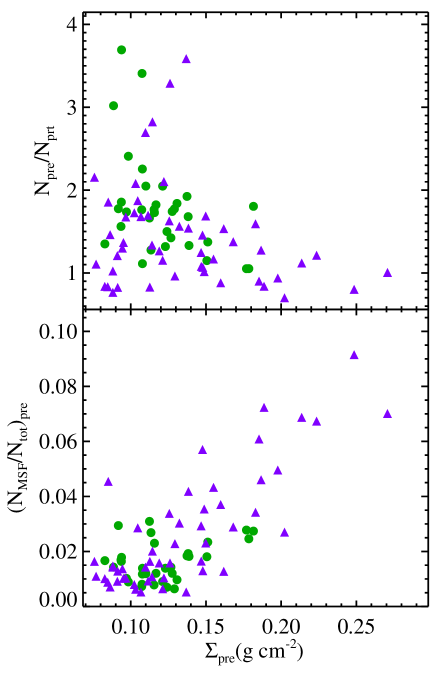
Figure 27: Number ratio of pre-stellar on proto-stellar sources (top), and of sources compatible with massive star formation on the total (bottom), as a function of median surface density of pre-stellar sources, estimated in the same 1-degree bin of Galactic longitude. Data are taken from Figure 26, panels $a$, $b$, and $c$. Data from the fourth and first Galactic quadrants are represented with purple triangles and green circles, respectively.

The fraction of sources exceeding the threshold necessary for massive star formation ($N_{\mathrm{MSF}}/N_{\mathrm{tot}}$) according to the prescription of Krumholz & McKee (2008) (see Section 6.3) is shown in panel $c$ of Figure 26, again separately for pre- and proto-stellar sources. As explained in Section 6.3, only starless sources are suitable for this analysis, and this fact is highlighted in the plot by connecting the proto-stellar distribution through a dashed line instead of a solid one. A few remarks can be made about this plot:

• The fraction of pre-stellar clumps potentially able to form massive stars $(N_{\mathrm{MSF}}/N_{\mathrm{tot}})_{\mathrm{pre}}$ is generally higher in the fourth rather than in the first quadrant. This can be seen also by plotting the mass vs radius diagram for the two quadrants separately, as in Figure 28: both quadrants denote, with respect to the two adopted density thresholds, a similar ability to form high-mass stars, but the fraction of pre-stellar sources in the fourth quadrant populating the Krumholz & McKee (2008) area is slightly larger.

• In the first quadrant, a relevant amount of pre-stellar sources which are massive and dense enough to give rise to possible high-mass star formation are found. In particular while Ginsburg et al. (2012), based on BGPS data, claim that no quiescent clumps with $M>10^{4}~{}M_{\odot}$ and $r<2.5$ pc are found between $6^{\circ}<\ell<90^{\circ}$ (confirmed by Svoboda et al., 2016, after an accurate analysis in the range $10^{\circ}<\ell<65^{\circ}$), in our catalogue we find 22 sources, located in the range $67^{\circ}<\ell<16^{\circ}$, that fulfil these criteria. To explain such a discrepancy, one should perform a dedicated analysis, which is beyond the scope of the present paper. Here we limit ourselves to emphasising two aspects. First, for all sources of this group the ambiguity about the heliocentric distance has been solved in favour of the “far” solution (the minimum distance in the group being $d=5979$ kpc, and 11 sources out of 22 have a distance in the catalogue $d>10$ kpc. A different distance estimate has a linear effect on radius, but a quadratic effect on the mass, and these in turn could potentially affect source classification. Second, the masses of Ginsburg et al. (2012) are estimated for a constant temperature of $T=20$ K (a value which is far from being representative of a starless clump, as seen in this paper), while in our case they are derived from a grey-body fit simultaneously with temperature: for the 22 sources in question, the derived temperatures are significantly lower than 20 K (with an average of 16.4 K), therefore leading to much higher values of mass. Indeed, at 1.1 mm (the wavelength used by Ginsburg et al., 2012), assuming a grey body temperature of 20 K instead of 13 K underestimates the mass by a factor $\sim 2$, independently from the choice of $\beta$. Svoboda et al. (2016) used a more accurate estimate of temperature, derived from NH₃ line observations of each source, which, in global terms, is still higher for pre-stellar sources (a median of 13.96 K against 11.7 K in our case, see Section 6.2). In addition to this, in the particular case of our 22 sources, grey body temperatures are found to be generally lower, with 16 of them having $T<10~{}K$. Such a temperature can be genuine but could be also attributed to a SED affected by problems in the original photometry or by relevant deficit of flux at the shortest wavelengths involved in the fit, due to multiplicity (see Section 3.1). A dedicated analysis is required for this group of sources to better define their physical conditions and confirm whether they might be genuine progenitors of massive proto-clusters, or simply statistical fluctuations in a huge catalogue.

• In the fourth quadrant, $(N_{\mathrm{MSF}}/N_{\mathrm{tot}})_{\mathrm{pre}}$ is found to increase towards inner longitudes ($\ell\gtrsim-35^{\circ}$).

• As expected, in general there is a direct relation between $N_{\mathrm{MSF}}/N_{\mathrm{tot}}$ for pre-stellar sources and the corresponding median surface density (for pre-stellar sources), shown in Figure 27, bottom panel .

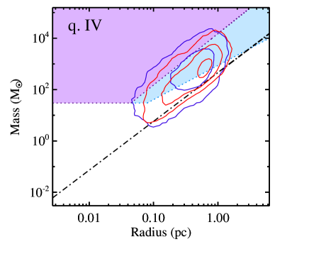
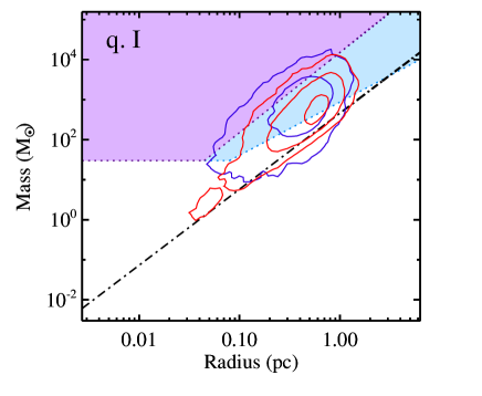
Figure 28: The same contour plots as in bottom left panel of Figure 7, but obtained separately for sources in the fourth (top) and in the first (bottom) Galactic quadrant, respectively.

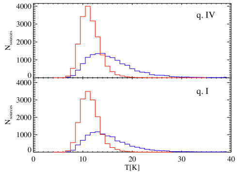
Figure 29: The same histogram as in Figure 5, but obtained separately for sources in the fourth (top) and in the first (bottom) Galactic quadrant, respectively.

We can now start analysing the behaviour of the evolutionary diagnostics. We begin with dust temperature, whose distribution is shown in Figure 26, panel $d$. We notice that the two Galactic quadrants do not present significant differences, as can also be seen in Figure 29, similar to Figure 5 but with the temperature distributions given separately for the fourth and first quadrant. If we compare the top and bottom panels of this figure, the distribution of proto-stellar sources in the fourth quadrant peaks at slightly higher temperatures with respect to the equivalent population in the first quadrant, with the average and median temperatures of $\bar{T}_{\mathrm{prt,IV}}=$16.2 K and $\tilde{T}_{\mathrm{prt,IV}}=15.3$ K in the fourth quadrant, and $\bar{T}_{\mathrm{prt,I}}=15.8$ K and $\tilde{T}_{\mathrm{prt,I}}=14.8$ K in the first quadrant, respectively. Notice, however, that the associated standard deviations of  5 K in all cases make this difference poorly significant from the statistical point of view. In the following, however, further slight differences between source properties in the two quadrants, globally indicating a more evolved stage of sources in the fourth quadrant, will be discussed.

No significant differences are found for the pre-stellar sources in the two quadrants ($\bar{T}_{\mathrm{pre,IV}}=12.0$ K vs $\bar{T}_{\mathrm{pre,I}}=11.9$ K, and $\tilde{T}_{\mathrm{pre,IV}}=11.8$ K vs $\tilde{T}_{\mathrm{pre,I}}=11.7$ K, respectively).

Figure 26, panel $d$ shows the median temperature as a function of the Galactic longitude. It can be seen that three strong local peaks ($\tilde{T}\geq 17$ K) at $-68^{\circ}$, $-61^{\circ}$, $-43^{\circ}$ are found in the fourth quadrant, while two dips ($\tilde{T}\leq 13$ K) at 47^∘, 57^∘ are found in the first one. However, these do not correspond to large source counts (Figure 26, panel $a$), indicating that they should not be considered as the main cause of the overall discrepancy between the two quadrants which, therefore is more indicative of a general trend.

Peaks and dips in the temperature distribution are found in the same longitude bins for $L_{\mathrm{bol}/M}$ and $L_{\mathrm{bol}}/L_{\mathrm{smm}}$ (Figure 26, panels $e$ and $f$, respectively). This is not surprising, given the tight relation between the temperature and these two indicators as suggested by Figure 18. A weaker correlation is seen with bolometric temperature (Figure 26, panel $g$).

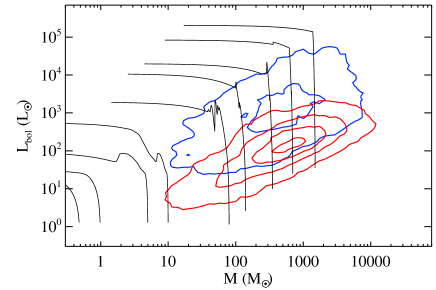
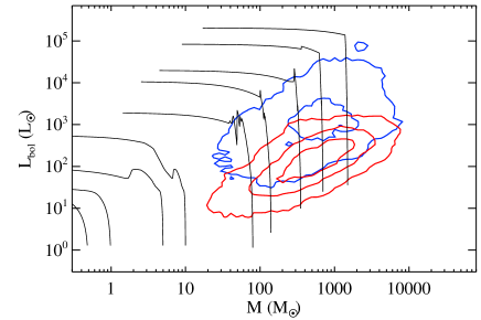
Figure 30: The same plot of $L_{\mathrm{bol}}/M$ as in Figure 12, but obtained separately for sources in the fourth (top) and in the first (bottom) Galactic quadrant, respectively.

Except for the features mentioned above, the global $L_{\mathrm{bol}}/M$ behaviour in the two quadrants does not appear very different, as corroborated by two observational facts:

• In Figure 30, in which the $L_{\mathrm{bol}}$ vs $M$, in form of density contours, is plotted separately for the two quadrants: the overall source distribution appears to be concentrated in the same region of the diagram, with respect to the evolutionary tracks of Molinari et al. (2008).

• The mean and median values of this ratio for proto-tellar objects, namely $[(L_{\mathrm{bol}}/M)_{\mathrm{prt,IV}}]_{\mathrm{med}}=2.7~{}L_{\mathrm{\odot}}/M_{\mathrm{\odot}}$ and $[(L_{\mathrm{bol}}/M)_{\mathrm{prt,I}}]_{\mathrm{med}}=2.3~{}L_{\mathrm{\odot}}/M_{\mathrm{\odot}}$, respectively, are very similar. They are reported also in Figure 23, together with other evolutionary indicators. The charts corresponding to the proto-stellar population of the two quadrants show only slight differences although, interestingly, these appear to be systematic: the fourth quadrant has larger $T$, $L_{\mathrm{bol}}/M$, $L_{\mathrm{bol}}/L_{\mathrm{smm}}$, and $T_{\mathrm{bol}}$, and lower $\Sigma$, which unequivocally indicate a (slightly) more advanced stage of evolution.

8.2 Spiral arms and star formation

The physical properties discussed in the previous section provided a first “1-dimensional” picture of how the sources of the Hi-GAL catalogue are distributed across the Milky Way. A more complete analysis also has to incorporate source distances to investigate their position in the Galactic plane, with respect to spiral arm topology, as already suggested by Figure 1. In the interest of completeness, we briefly touch here on this topic, while for more details and and an extensive discussion we refer the reader to Ragan et al. (2016).

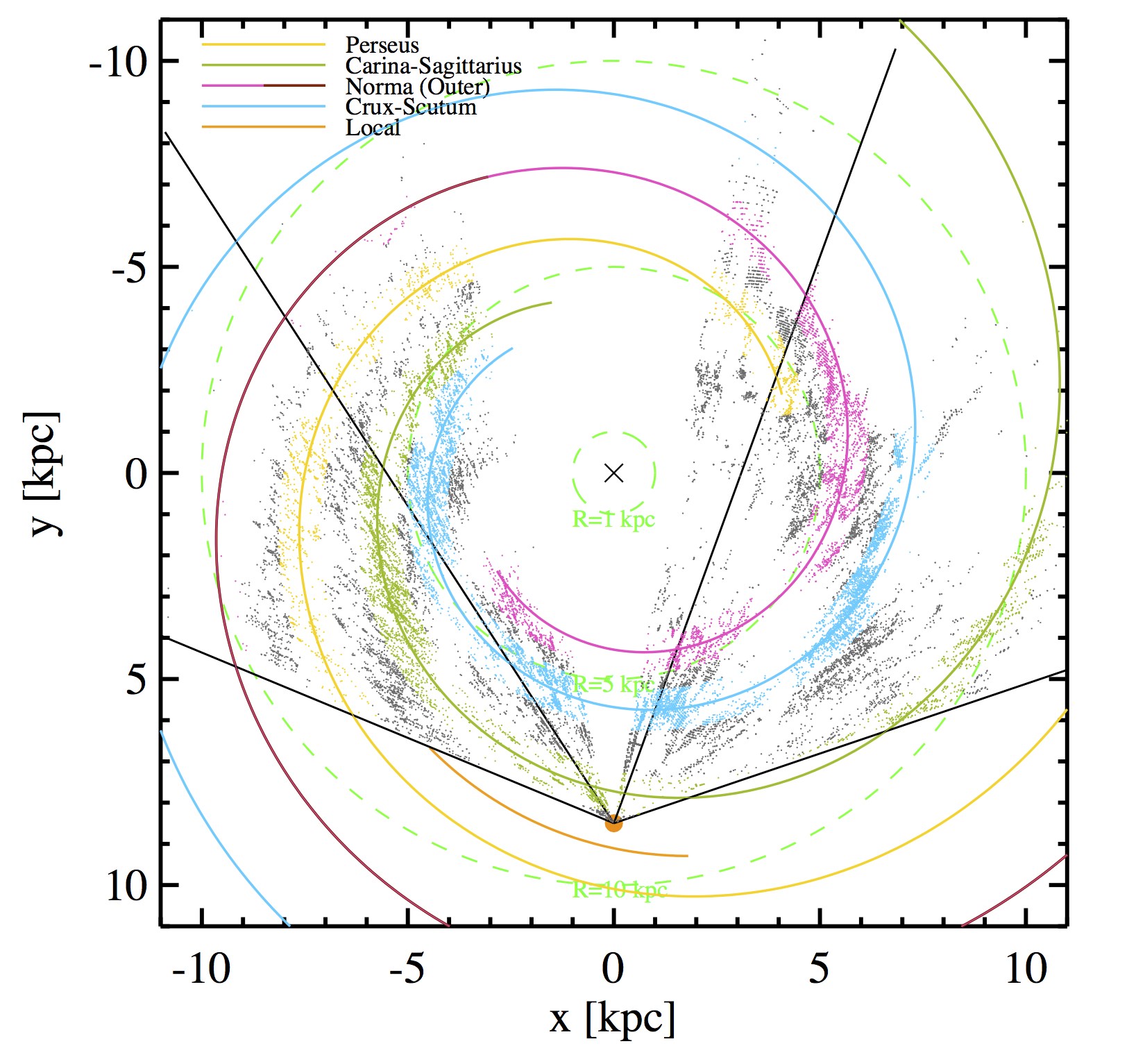
Figure 31: The same as Figure 1, but with different colours for dots representing sources: positions within a distance 0.5 pc from the theoretical position of an arm are assigned to it and displayed with the same colour (with no reference to the starless vs proto-stellar classification). The remaining sources, found at “inter-arm” locations, are displayed in grey.

In Figure 31, as in Figure 1, we show the overall distribution of the Hi-GAL clumps along the Galactic plane as well as the location of the spiral arms according to the model of Hou et al. (2009). In this new figure, however, we also make an attempt to associate clumps with spiral arms. To this end, we use an arm width of 1 kpc, then a source-to-arm association distance of 0.5 kpc (cf. Eden et al., 2013). According to this criterion, 21996 sources out of 36535 considered for this analysis (i.e., those provided with a heliocentric distance estimate) are associated with the arms. In addition, 14539 are classified as “inter-arm”, thus a $\sim 2:3$ ratio, significantly different from the 1:7 expected by simulations of Dobbs & Bonnell (2007), but in better agreement with the observational evidence of Eden et al. (2013), namely 21:38 for BGPS sources between $\ell=37^{\circ}.8$ and $42^{\circ}.5$. However, we should make the reader aware that this association between sources and arms and the consequent results are strongly affected by heliocentric distance determination, which is still a critical point in our analysis. While a new set of Hi-GAL source distances based on an improved algorithm is expected (Russeil et al., in preparation), cross-checks can be carried out (although on a relatively small number of cases) with distances quoted for objects in common with surveys such as ATLASGAL (Wienen et al., 2015) or BGPS (Ellsworth-Bowers et al., 2015) (see Appendix D). In this way a distance estimate external to our catalogue and considered more reliable can be assumed to easily re-scale the distance-dependent source properties quoted in our catalogue.

As already evident from Figure 1, overdensities of source counts do not always correspond to arm locations. This certainly also depends on the spiral arm model of choice (see, e.g., Ragan et al., 2016) but, even more, is primarily inherent to the set of estimated distances. As a matter of fact, different spiral arm models will provide different solutions so, for a certain model, a source will result being “on-arm” while, for another, it might turn out to be “off-arm”. Moreover, the on-off location of clumps with respect to spiral arms will also strongly depend on kinematic distances, which are notoriously limited - by their intrinsic uncertainties - in their ability of delineating the morphology of the arms. Therefore, the prescription we adopted to associate Hi-GAL clumps to spiral arms produces sharp and unnatural separations between on-arm and off-arm populations (see Figure 31), which affects a possible comparison of the two, as well as the remaining analysis. This aspect was already evident in Roman-Duval et al. (2009), who examined the same spectroscopic survey, namely GRS, that we use here to determine distances in the first Galactic quadrant: they found that only 63% of ¹³CO emission can be associated to spiral arms, while several bright and large structures fall in “inter-arm” gaps.

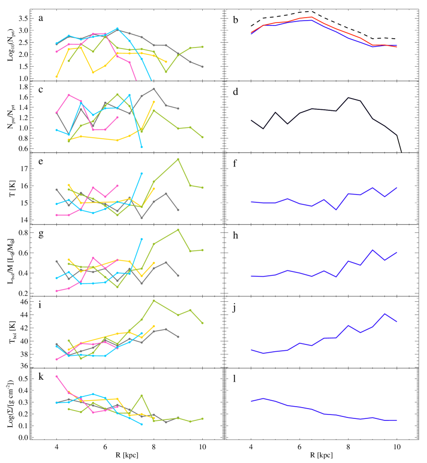
Figure 32: Number and physical properties of proto-stellar clumps with a distance estimate, in bins of Galactocentric radius (bin width is 0.5 kpc). In left panels, different quantities are plotted separately by spiral arms (see Figures 1 and 31 for colour coding) with the addition of “inter-arm” sources (in grey). In right panels the overall sample of proto-stellar sources is considered. In detail, panel $a$ shows the logarithm of the number of proto-stellar sources, while panel $b$ shows the sum of them (blue solid line); the counts of pre-stellar and the sum of pre-+proto-stellar are also reported as red solid and black dashed lines, respectively. In panel $c$ the number ratio of pre- over proto-stellar sources is reported, while in panel $d$ the same quantity is computed and reported for the entire source population (black line). Panels $e$, $g$, $i$, and $k$ are similar to panel $c$, but for dust temperature, logarithm of the luminosity/mass ratio, bolometric temperature, ad logarithm of surface density respectively. Correspondingly, panels $f$, $h$, $j$, and $l$ report the same distributions, but calculated over the entire population of proto-stellar sources.

With these caveats in mind, we present some statistics based on grouping sources belonging to the same arm, and distributed at a different Galactocentric radius $R$. In Figure 32, panel $a$, first of all we show the number statistics of proto-stellar objects, which the other panels are based on. This information is useful to understand the reliability of statistics presented in the other panels: clumps are counted in bins of 0.5 kpc of Galactocentric radius, and bins poorly populated (i.e. $<50$ sources) are ignored in the following. The overall number of proto-stellar sources as a function of $R$ is reported in panel $b$, together with the same curve for pre-stellar sources (used to build the plot in panel $d$) and for the sum of the two classes. A direct comparison of the latter with the Galactocentric radius distribution of ATLASGAL sources presented by Wienen et al. (2015) is not straightforward. This is because, in that case, the plot is split between the first and fourth Galactic quadrants, and because counts are expressed in surface density, therefore normalised by the area. As in Wienen et al. (2015), a peak is found around 4.5 kpc, corresponding to the peak of the light blue line in panel $a$, so that we agree with those authors that this enhancement corresponds to the intersection of the Crux-Scutum arm and the Galactic bar in the first quadrant (see also Nguyen Luong et al., 2011; Motte et al., 2014). Another peak (the largest we find) is encountered around 6.5 kpc, and again it is mostly due to the Crux-Scutum arm, but in particular to its portion in the fourth quadrant. In both cases, the curve of “inter-arm” clumps closely follows that of the Crux-Scutum arm and strongly contributes to the aforementioned peaks, corroborating the fact that, in many locations, the distinction between “on-arm” and “inter-arm” locations is quite artificial due to the method we used to identify them. Finally, at $R\sim 10$ kpc (this distance is not probed by Wienen et al., 2015), sources of the Carina-Sagittarius arm produce a peak which is mirrored in the overall source distribution as a plateau interrupting a decreasing trend found over a range of 2.5 kpc.

In panel $c$ the ratio between pre-stellar and proto-stellar clumps $N_{\mathrm{pre}}/N_{\mathrm{prt}}$ (discussed in Section 8.1 as a function of Galactic longitude) is shown in bins of $R$ for different arms and for the “inter-arm” sources. Values range from 0.7 to 1.8, but no specific trends are found either for the behaviour of individual arms or in the comparison between “on-arm” and “inter-arm” sources. Therefore, no suggestions come from this plot about a possible role of spiral arms in triggering or regulating star formation, confirming the conclusions of Eden et al. (2013) and Ragan et al. (2016). Analogously, the distributions of three evolutionary indicators such as median dust temperature, bolometric luminosity/mass ratio, and bolometric temperature of proto-stellar sources (panels $e$, $g$, and $i$, respectively) show a high degree of scatter and no substantial differences between arm and “inter-arm” sources. A recognizable trend is present in the distribution of median bolometric temperatures, which generally increases at increasing $R$ for all arms and for the inter-arm component as well. This is more evident in the overall behaviour shown in panel $j$, even ignoring bins at $R>8$ kpc, which are dominated by the Carina-Sagittarius arm in the fourth quadrant, and which are generally characterised by high values for the evolutionary indicators as seen also in panels $e$, $g$, $f$ and $h$, although based on relatively poor statistics (see panel $a$). Finally, the distributions of surface densities reported in panel $k$ show a slightly decreasing trend with $R$, as recognised in all curves and in the overall distribution (panel $l$). A linear fit to the overall distribution between 4.5 and 9 kpc to the latter gives the relation $\log_{10}(\Sigma/(\mathrm{g~{}cm^{-2}}))=0.50-0.04~{}(R/\mathrm{kpc})$. A much stronger decrease of clump surface peak is claimed by Zahorecz et al. (2016), who found a drop of three orders of magnitude over the range 0-13 kpc, but this quantity cannot be directly compared with our average surface density. More generally, encountering less dense clumps at farther distances from the Galactic centre is in agreement with the result of Ragan et al. (2016): these authors define a “star forming fraction” as the number ratio (based on the present catalogue) between proto-stellar and all clumps, and find a general trend decreasing with increasing $R$ (with a slope of -0.025). In other words, a correlation between the gradual decrease of star formation activity at large Galactocentric radii and the decrease of the clump densities (i.e. of material available for gravitational collapse) can be hypothesised.

9 Summary

We presented the physical catalogue of Hi-GAL compact sources extracted in the inner Galaxy (in the longitude range between $\ell=-71^{\circ}$ and $\ell=67^{\circ}$). First we described how sources were selected from the Hi-GAL five-band photometric catalogue and how their physical properties were estimated. To this aim we illustrated how:

1. Five single-band photometric catalogs of Molinari et al. (2016a) were merged, based on simple positional associations. A total of 100922 SEDs eligible for grey body fit were selected and considered for subsequent analysis, 57065 of which included a heliocentric distance estimate (no distances are available in the central part of the Galaxy $-10.2^{\circ}<\ell<14.0^{\circ}$).

2. A targeted flux extraction at 160 and 70 $\mu$m has been performed for sources missing a flux at these bands. Sources remained with only three Hi-GAL fluxes have been reported in a “lower-reliability” list. Furthermore, the MSX, WISE, MIPSGAL, ATLASGAL, and BGPS catalogues have been searched for possible geometric counterparts, to extend the spectral coverage of the SEDs.

3. After SED building and filtering, the 24584 sources containing a flux at 70 $\mu$m have been classified as proto-stellar, while the remaining 76338 sources as starless. Furthermore, based on subsequent SED fitting and mass computation, starless sources have been classified as gravitationally bound (pre-stellar) or unbound (16667 and 59671, respectively). Both these criteria are applied directly and uniquely on photometric data, and for this reason are prone to be refined in future using other observational evidence. Furthermore, they can not remove completely a certain degree of contamination among different evolutionary classes.

4. A grey body spectrum has been fitted to SEDs, to obtain the average temperature and the total mass of a clump (in case of available distance, otherwise at least the clump surface density has been derived, taking the source diameter at 250 $\mu$m as a reference size). The bolometric luminosity has been derived for sources provided with a distance estimate, while the bolometric temperature has been obtained for all sources.

Once the physical properties of the sources were derived, we explored the distributions of these observables, their mutual relations with a possible evolutionary scenario, and their possible connection with the Galactic large scale structure. Main results are summarised below:

1. Based on their size, the sources in this catalogue are in most cases classifiable as clumps. For a given distance, proto-stellar clumps are found to be on average more compact than starless ones. Consequently, the former are found to be generally denser than the latter.

2. A significant amount of sources, both pre- and proto-stellar, is found to fulfil one or more criteria for compatibility with high-mass star formation. This sample can be extracted for large programs of follow-up observations aimed to clarify the internal structure of dense clumps and put observational constraints on models of high-mass star formation.

3. The mass function of proto-stellar sources falling in a relatively narrow ($\Delta d=0.5$ kpc) distance range appears generally wider than that of pre-stellar sources, due to completeness effects at low masses, and to relative deficit of pre-stellar clumps at high masses (in turn likely due to evolutionary effects). As a consequence of this, the power-law slope of the pre-stellar function is systematically steeper than that of the proto-stellar one. Finally, no systematic bias seems to affect the mass function slope at increasing heliocentric distance.

4. The clump average temperature, estimated over the range $160~{}\mu$m$\leq\lambda\leq 500~{}\mu$m (so with no reference to the presence of counterparts at shorter wavelengths) and representing the physical conditions of the outer part of the clump structure, acts as an evolutionary indicator: the median temperature for pre-stellar clumps is 11.7 K, while for proto-stellar sources is 15.1 K. However a high degree of overlap between the two populations remains and the combined use of further evolutionary indicators is then recommended to reduce such degeneracy.

5. We used the bolometric luminosity and its ratios with the clump mass and the sub-millimetre luminosity, together with the bolometric temperature, as further evolutionary indicators. An acceptable degree of separation between pre- and proto-stellar populations is found by analysing the distributions of these observables. Since the proto-stellar sources span a wide range of evolutionary stages, we tried to identify possible candidates to represent both the earliest and the latest stages that we are able to probe with Hi-GAL. On the one hand, we found that sources dark in the MIR may play the former role only in part, while, on the other hand, sources with $L_{\mathrm{bol}}/M>22.4L_{\odot}/M_{\odot}$ represent the right tail in the distribution of all evolutionary indicators, and are compatible, for temperature and colours, with the stage of H ii regions, although this requires further observational evidences to be gathered.

6. The behaviour of surface density with respect to clump evolution shows, in general, an increase from the pre- to the proto-stellar phase, and a decrease (but with a large spread of values) in the most evolved proto-stellar objects, corresponding to the envelope clean-up phase.

7. Regarding the source distributions with Galactic longitude, local excesses of sources are encountered in correspondence with spiral arm tangent points or star forming complexes. A low number ratio between pre- and proto-stellar sources, evaluated in bins of longitude, found in correspondence with high median surface density in the same bins ($\Sigma>0.2$ g cm^-2) may suggest a short lifetime of high-density clumps in the pre-stellar stage. Despite of this, we find a conspicuous number of pre-stellar cores compatible with high-mass star formation, especially in the fourth quadrant.

8. No large differences are found between medians of clump evolutionary indicators in the fourth and in the first quadrant. However, although differences are quite small, median temperature, luminosity over mass ratio, bolometric over sub-mm luminosity ratio, and bolometric temperature are larger in the fourth than in the first quadrant.

9. Although the set of distances we adopt does not produce, in some regions of the Galactic plane, a source pattern showing well definite spiral arms, we made a tentative assignment of sources to spiral arms modelled by Hou et al. (2009). “On-arm” and “inter-arm” populations show no relevant differences either in the pre- over proto-stellar number ratio or in the median values of the evolutionary indicators. This result could suggest a negligible impact of spiral arms in triggering star formation. However, this result is biased by the uncertainties affecting source distance estimations and consequently association with spiral arms.

10. While temperature and luminosity over mass ratio do not show clear trends as a function of the increasing Galactocentric radius, a slightly increasing trend is found for median bolometric temperature, and a slightly decreasing one for the median surface density.

In conclusion, the aim of this paper is to give a first look at the huge amount of information contained in the Hi-GAL physical catalogue of the inner Galaxy. Papers based on data taken from this catalogue have been already published (Ragan et al., 2016; Persi et al., 2016), as well as observational programs submitted for (and also partially observed with) ALMA. A number of papers exploiting this catalogue, or aiming at completing it in the outer Galaxy, are in preparation at present, and will contribute to deepen and refine the conclusions of this work.

Appendix A Description of physical catalogue

The HI-GAL physical catalogue for the inner Galaxy is hosted in the VIALACTEA knowledge base (VLKB, Molinaro et al., 2016), and is arranged in two tables (high- and low-reliability SEDs) both containing the same columns, defined as follows:

• Column [1], ID: running number (starting from 1 in the high-reliability table and continuing in the low-reliability one).

• Column [2], DESIGNATION: string composed by “HIGAL”, “BM” (which stays for “band-merged”) and Galactic coordinates of the sources, chosen as the coordinates of the shortest-wavelength available Hi-GAL counterpart.

• Columns [3], GLON, and [4] GLAT: Galactic longitude and latitude, respectively, assigned to the source, chosen as the coordinates of the shortest-wavelength available Hi-GAL counterpart.

• Columns [5], RA, and [6], DEC: the same as in columns [3] and [4], respectively, but for source Equatorial coordinates.

• Column [7], DESIGNATION_70: designation of the PACS $70~{}\mu$m counterpart (if available), as defined in the catalogue of Molinari et al. (2016a). The null string (in case of a missing counterpart at this band) is “-”.

• Column [8], F70: flux density (hereafter flux) of the PACS $70~{}\mu$m counterpart (if available), in Jy, as quoted by Molinari et al. (2016a). The null value is 0.

• Column [9], DF70: uncertainty associated to the flux in column [8] as quoted by Molinari et al. (2016a). The null value is 0.

• Column [10], F70_TOT: sum of fluxes of all PACS $70~{}\mu$m counterparts (if available) lying inside the half-maximum ellipse of the source detected by CuTEx in the SPIRE $250~{}\mu$m maps. By definition, $F_{\mathrm{70,tot}}\geq F_{\mathrm{70}}$. The null value is 0. This is the flux at $70~{}\mu$m actually used to estimate the source bolometric luminosity (Section 4) and temperature (Section 7.2).

• Column [11], DF70_TOT: uncertainty associated to the flux in column [10], obtained as the quadratic sum of uncertainties on single fluxes. The null value is 0.

• Column [12] F70_ADD: flux of the closest PACS $70~{}\mu$m counterpart (if available) found through targeted source extraction at a detection threshold lower than in Molinari et al. (2016a) where $F_{\mathrm{70,tot}}=0$ (column[11]), as described in Section 3.5. The null value is 0.

• Column [13], DF70_ADD: uncertainty associated to the flux in column [12]. The null value is 0.

• Column [14], F70_ADD_TOT: sum of fluxes of all PACS $70~{}\mu$m counterparts (if available) found through targeted source extraction at a detection threshold lower than in Molinari et al. (2016a) where $F_{\mathrm{70,tot}}=0$, and lying inside the ellipse at $250~{}\mu$m (as for column [10]). The null value is 0. This is the flux at $70~{}\mu$m actually used to estimate the source bolometric luminosity and temperature where $F_{\mathrm{70,tot}}=0$.

• Column [15], DF70_ADD_TOT: uncertainty associated to the flux in column [14], estimated as for column [11]. The null value is 0.

• Column [16], ULIM_70: 5-$\sigma$ upper limit in the PACS $70~{}\mu$m band, estimated where both $F_{\mathrm{70,tot}}=0$ (column [10]) and $F_{\mathrm{70add,tot}}=0$ (column[14]).

• Columns [17], DESIGNATION_160, [18], F160, and [19], DF160: the same as columns [7], [8], and [9], respectively, but for the PACS $160~{}\mu$m band.

• Columns [20], F160_ADD, and [21], DF160_ADD: the same as columns [12], and [13], respectively, but for the PACS $160~{}\mu$m band.

• Column [21], ULIM_160: 5-$\sigma$ upper limit in the PACS $160~{}\mu$m band, estimated where both $F_{\mathrm{160}}=0$ (column [18]) and $F_{\mathrm{160add}}=0$ (column [20]).

• Columns [22], DESIGNATION_250, [23], F250, and [24], DF250: the same as columns [7], [8], and [9], respectively, but for the SPIRE $250~{}\mu$m band.

• Columns [25], DESIGNATION_350, [26], F350, and [27], DF350 : the same as columns [7], [8], and [9], respectively, but for the SPIRE $350~{}\mu$m band.

• Column [28], FSC350: SPIRE $350~{}\mu$m flux “scaled” as mentioned in Section 3.1. Further details on the method are provided, e.g., in Giannini et al. (2012). Scaling is not performed when the source size differs by less than a factor $\sqrt{2}$ from the instrumental beam size at this wavelength.

• Column [29], DFSC350: uncertainty associated to the flux in column [28].

• Columns [30], DESIGNATION_500, [31], F500, [32], DF500, [33], FSC500, and [34], DFSC500: the same as columns [25], [26], [27], [28], and [29], respectively, but for the SPIRE $500~{}\mu$m band.

• Column [35], DESIGNATION_21: designation of the MSX $21~{}\mu$m counterpart (if available), as defined in the MSX point source catalogue. The null string (in case of a missing counterpart at this band) is “-”

• Column [36], F21: flux of the closest MXS $21~{}\mu$m counterpart (if available within the adopted matching radius), in Jy. The null value is 0.

• Column [37], DF21: uncertainty associated to the flux in column [36]. The null value is 0.

• Column [38], F21_TOT: sum of fluxes of all MXS $21~{}\mu$m counterparts (if available) lying inside the ellipse at $250~{}\mu$m (as done for column [10]). The null value is 0.

• Column [39], DF21_TOT: uncertainty associated to the flux in column [38], computed as for column [11]. The null value is 0.

• Columns [40], DESIGNATION_22, [41], F22, [42], DF22, [43], F22_TOT, and [44], DF22_TOT: the same as columns [35], [36], [37], [38], and [39], but for the WISE $22~{}\mu$m band.

• Column [45], DESIGNATION_24: designation of the MSX $24~{}\mu$m counterpart (if available). A string beginning with “MG” identifies a source taken from the catalog of (Gutermuth & Heyer, 2015), while a string beginning with “D” identifies a source specifically detected in this work, (cf. Section 3.3). Furthermore, lack of a source due to saturation is identified with the “satutared” string.

• Columns [46], F24, [47], DF24, [48], F24_TOT, and [49], DF24_TOT: the same as columns [36], [37], [38], and [39], respectively, but for the MIPSGAL $24~{}\mu$m band. In column [46], in case of saturation (see column [45]) a null value -999 is quoted.

• Column [50], DESIGNATION_870: designation of the ATLASGAL $870~{}\mu$m counterpart (if available). A string beginning with “G” identifies a source taken from the catalog of Csengeri et al. (2014) while the string "CuTEx" identifies a source specifically detected for this work, as explained in Section 3.3. The null string (in case of a missing counterpart at this band) is “-”.

• Columns [51], F870, and [52], DF870: the same as columns [46] and [47], respectively, but for the ATLASGAL $870~{}\mu$m band.

• Column [52], DESIGNATION_1100: designation of the BGPS $1100~{}\mu$m counterpart (if available), as defined in the BGPS catalogue (Ginsburg et al., 2013). The null string (in case of a missing counterpart at this band) is “-”.

• Columns [53], F1100, and [54], DF1100: the same as columns [46] and [47], respectively, but for the BOLOCAM $1100~{}\mu$m band.

• Columns [54], DFWHM250: circularised and (if the circularised size exceeds the instrumental beam size of a factor $\sqrt{2}$) beam-deconvolved size of the sources as estimated by CuTEx in the $250~{}\mu$m band, in arcseconds.

• Columns [55], DIST: kinematic distance of the source, in pc (Russeil et al., 2011). In case of distance ambiguity, it represents the final choice between the “near” and the “far” estimates, reported in the two next columns. The null value, in case of unavailable distance estimate, is 0.

• Columns [56], NEAR_DIST, and [57], FAR_DIST: “near” and “far” kinematic distance estimates of the source, in pc. The null value is 0.

• Column [58], DIST_FLAG: flag indicating the quality of the distance “near”/“far” ambiguity solution. If an external indicator is used to take the decision, the flag is “G”, otherwise it is “B”, and the “far” distance is assigned to the source by default (see Section 3.4). The null value, in case of unavailable distance estimate, is “-”.

• Column [59], DIAM: source linear diameter, in pc, obtained combining columns [54] and [55].

• Column [60], M_LARS: Larson’s mass, in Solar masses, evaluated as described in Section 3.5. The null value, in case of unavailable distance, is 0.

• Column [61], FIT_TYPE: flag indicating if the expression of the grey body fitted to the source SED is given by Equation 1 (“thick” case, “Tk” flag) or Equation 4 (“thin” case, “Tn” flag).

• Column [62], EVOL_FLAG: flag indicating the evolutionary classification of the source (0: starless unbound; 1: pre-stellar; 2: proto-stellar).

• Column [63], MASS: clump total mass, in units of Solar masses, derived fitting a grey body to the source SED. In case of unavailable distance, the fit is performed anyway assuming a virtual distance of 1 kpc, and the corresponding mass is quoted as a negative value.

• Column [64], DMASS: uncertainty associated to the mass in column [63].

• Column [65], TEMP: dust temperature of the clump, in K, derived from the grey-body fit.

• Column [66], DTEMP: uncertainty associated to the temperature in column [65].

• Column [67], LAM_0_TK: value of $\lambda_{0}$ (see Equation 1), in $\mu$m, derived from the grey-body fit. The null value, corresponding to the value “Tn” of the flag FIT_TYPE, is 0.

• Column [68], L_BOL: bolometric luminosity, in units of solar luminosity, estimated as described in Section 4. As in the case of the mass, for sources devoid of distance estimate a luminosity corresponding to the virtual distance of 1 kpc is calculated and quoted as a negative value.

• Column [69], LRATIO: ratio between bolometric luminosity in Column [67] and its fraction computed over the range $\lambda\geq 350\mu$m.

• Column [70], T_BOL: bolometric temperature, in K, calculated based on Equation 5.

• Column [71], SURF_DENS: surface density, in g cm^-2, calculated dividing the mass in Column [63] by the area of the circle with the diameter in Column [59]. Where the distance is unavailable, this quantity can be evaluated anyway, assuming a whatever virtual distance for intermediate calculations, and starting from Column [54] instead of [59].

Appendix B Possible Mid-infrared associations of starless Hi-GAL sources

In Section 3.5 we defined the classification of Hi-GAL sources in starless and proto-stellar, based on the absence or the presence of a detection at 70 $\mu$m, respectively. For the former ones, possible associations with MIR point sources are considered spurious, and are not taken into account for deriving the bolometric luminosity and temperature. To ascertain how reliable is this assumption, we performed two different tests.

The first test consisted in checking the impact of possible foreground MIR point sources on the incidence of chance associations with Hi-GAL sources. We chose eight Hi-GAL $4^{\circ}\times 1.4^{\circ}$ fields, centered on longitudes $\ell=-60^{\circ},-40^{\circ},-20^{\circ},-10^{\circ},10^{\circ},20^{\circ},40^{\circ},60^{\circ}$, respectively, and latitude $b=0^{\circ}$, so well inside the PACS-SPIRE common science area. First, we identified all sources having a detection at 160 $\mu$m and at 21 and/or 22 and/or 24 $\mu$m, but with no detection at 70 $\mu$m, i.e. the sub-sample of the entire starless population which might be misclassified in case of a too faint flux at 70 $\mu$m. We further restricted the investigated box area to the limits given by the maximum and minimum of longitude and latitude of the selected sources, and counted the total amount $N_{\mathrm{MIR}}$ of MSX, WISE, and MIPSGAL sources falling within such area. Then we randomly dispersed $N_{\mathrm{MIR}}$ points across the area, and performed the association with the selected starless Hi-GAL sources as described in Section 3.3. Finally, for each field we compared the number of associations $N_{\mathrm{rnd}}$ found with that of the actual associations between the selected Hi-GAL starless sources and MIR catalogue sources ($N_{\mathrm{cat}}$); in Figure 33, red circles represent the obtained statistics, with $N_{\mathrm{rnd}}/N_{\mathrm{cat}}$ being $>75\%$ in all cases. This suggests that most of the associations found between starless Hi-GAL sources and MIR catalogues can be explained as a chance alignment along the line of sight.

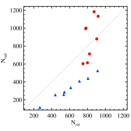
Figure 33: Comparison between the number $N_{\mathrm{cat}}$ of Hi-GAL sources (in each of eight different test fields, see text) found to be associated to MIR counterparts (being the total number of MIR sources $N_{\mathrm{MIR}}>N_{\mathrm{cat}}$) and the number $N_{\mathrm{rnd}}$ of associations established between the same Hi-GAL sources and $N_{\mathrm{MIR}}$ positions randomly dispersed in the same field. Red circles represent the statistics of starless sources detected at 160 $\mu$m, while blue triangles represent proto-stellar sources.

On the other hand, MIR counterparts found for proto-stellar sources should be considered as a more genuine effect. In fact, repeating the procedure described above on proto-stellar sources found in the test fields, we find an association rate smaller than $60\%$ in all cases, suggesting that, unlike the starless case, the real spatial disposition of MIR sources follows more closely the one of Hi-GAL proto-stellar objects, so cases of chance associations are expected to be less frequent.

The second test directly involves the photometry of the sources. The question arises whether the failed detection at 70 $\mu$m is caused by the fact that the SED is in the Wien regime of the grey body at this wavelength, emitting a too small flux to be detected with PACS, or it is due to lack of sensitivity, such that the emission at 70 $\mu$m is in excess of that expected from a grey body at given temperature, albeit remaining below the flux threshold of the instrument.

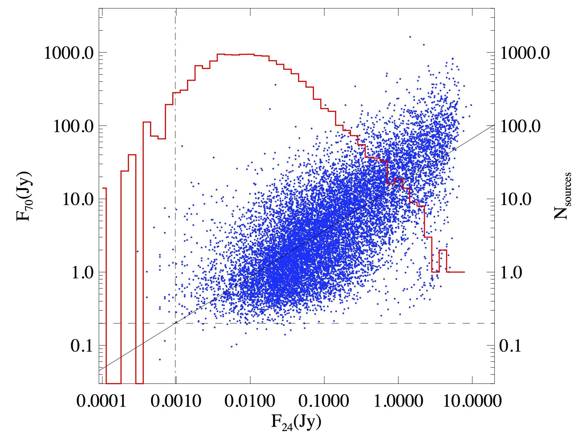
Figure 34: Scatter plot of flux at $70~{}\mu$m vs flux at $24~{}\mu$m for proto-stellar sources of the Hi-GAL catalogue provided with both these fluxes (blue dots). The solid line represents the power-law fit to the displayed points (see text). The horizontal black line represents the limit flux of 0.2 Jy at $70~{}\mu$m, while the vertical dotted-dashed line corresponds to the abscissa of the intersection of the previous line with the power-law fit. The red line is the histogram of flux at $24~{}\mu$m of sources with detection at $160~{}\mu$m and no detection at $70~{}\mu$m, plotted with respect to the $y$ axis reported on the right side of the box.

To investigate this issue, first we plot $F_{70}$ vs $F_{24}$ for proto-stellar sources (Figure 34). An overall correlation between the two fluxes is seen (cf with Spitzer literature, e.g. Young et al., 2005; Strafella et al., 2010), so that for this class of objects low PACS fluxes are expected in correspondence of low MIPS fluxes. Fitting a power law $F_{70}=a\,(F_{24})^{b}$ to the plotted data gives $a=15.7\pm 0.01$ and $b=0.63\pm 0.01$. Most of our sources have $F_{70}>0.2$ Jy, so that the corresponding $F_{24}$ suggested by the fit would be 0.001 Jy. This implies that, in principle, a source with $F_{24}>0.001$ Jy should be observable with PACS at 70 $\mu$m as well. Nevertheless, only the 3% of sources detected at 24 $\mu$m and 160 $\mu$m and not detected at 70 $\mu$m (histogram in Figure 34) has $F_{24}<0.001$ Jy, while for the rest a counterpart at 70 $\mu$m, according with the general trend of the other sources, should be detectable. Even increasing, to be more conservative, the threshold on $F_{70}$ to the 90% completeness limit for this band quoted by Molinari et al. (2016a), namely $\sim 0.5$ Jy, only 25% of MIPS sources would be fainter than the corresponding limit flux $F_{24}=0.004$ Jy, leaving the remaining ones to be likely chance associations.

We conclude that both tests discourage to consider a positional match between a Hi-GAL source undetected at 70 $\mu$m and a MIR source as a genuine physical association in most cases. It is noteworthy that in literature, before the release of Herschel catalogues, the pre- vs proto-stellar nature of sub-mm sources was ascertained just through simple spatial association with MIR counterparts, hence suffering of possible chance alignment contamination (e.g., Csengeri et al., 2014), all the more considering the large gap in wavelength between the two bands associated ($\lambda\sim 20~{}\mu$m to $\lambda\geq 870~{}\mu$m).

Appendix C Distance bias on source property estimation and interpretation

Whereas studying a single star forming region or complex it is possible to assume a single global distance estimate for its compact source population, a Galactic plane survey as Hi-GAL inevitably contains an extraordinary variety of distances superposed along the same line of sight. In Section 6.1 we already illustrated how such a variety produces a large spread of source physical sizes corresponding to the angular extent of the compact sources, in turn implying substantial consequences on their structural classification. Other source physical properties, however, may turn out to be strongly biased by distance effects. A systematic study of these effects will be published in Baldeschi et al. (2017). Here we limit ourselves to a few considerations related to this issue.

C.1 Source confusion and classification

The first issue originates from the simple concept of perspective confusion of two (or more) sources with a given physical separation, as their heliocentric distance increase, so that their angular separation decreases accordingly. Keeping in mind the classification of proto-stellar vs. starless sources introduced in Section 3.5, one can imagine the basic case in which two sources, quite close each other in the sky and belonging to these two different classes, are virtually placed at an increasing heliocentric distance and “re-observed”, until they get confused at the Herschel resolution. The 70 $\mu$m flux determining the proto-stellar classification of the former source would be, in this case, assigned to the new unresolved source including also the original starless companion, making it globally flagged as proto-stellar. On the one hand, this classification would remain true in principle, as such a structure, in fact, would have a proto-stellar content. On the other hand, the mass actually involved in the star formation activity would be (even significantly) smaller than the value quoted for the entire clump mass. This would result, at large distances, in an overestimate of the mass assigned to proto-stellar structures (see also Hatchell & Fuller, 2008).

To try to quantify this effect, we performed a simple test, considering all the sources of our Hi-GAL catalogue located at $d<4$ kpc, and ideally moved all of them at a larger distance $d\textsf{'}$, estimating the corresponding decrease of their mutual angular separations. Given a pair of sources $i$ and $j$, located at their original distances $d_{i}$ and $d_{j}$ and separated in the sky by an angle $\varphi_{0}$, if they are virtually moved away to a distance $d\textsf{'}>\max(d_{i},d_{j})$, the new simulated angular separation would become

$$\varphi\textsf{'}=\varphi_{0}\frac{\left(d_{1}+d_{2}\right)}{2d\textsf{'}}\;.$$ (6)

Probing virtual distances in steps of 1 kpc, starting from $d\textsf{'}=5$ kpc, and assuming that two (or more) sources get confused when their mutual angular separation becomes smaller than the SPIRE beam at $250~{}\mu$m (i.e. for $\varphi\textsf{'}<18\arcsec$), a trend for the ratio (both in number and in total mass) of sources classified as proto-stellar over the whole source sample has been estimated.

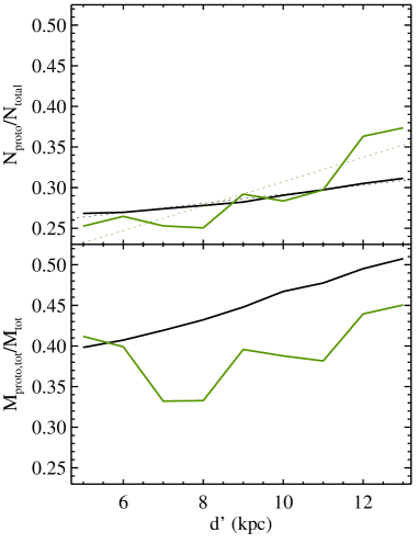
Figure 35: Distance bias affecting the estimate of the global fraction of proto-stellar sources, both in number (top) and mass (bottom). All the Hi-GAL sources located within $d=4$ kpc have been virtually moved to larger distances, starting from $d\textsf{'}=5$ kpc, and their mutual separation reevaluated accordingly. Sources getting confused after this operation define a new unresolved source which assumes a proto-stellar character if at least one of its original components was proto-stellar; the new mass is simply calculated as the sum of the masses of the original sources. Top: black solid line, fraction of proto-stellar sources over the total amount of sources, as a function of the new simulated distance. Black dotted line: linear best fit of the previous one. Green solid line: the same quantity calculated for the real Hi-GAL sources encountered at the considered distances (in bins 1 kpc-wide, centered at multiples of 1 kpc). Green dotted line: linear best fit to the previous one. Bottom: the solid lines are the same as in the top panel, but for the proto-stellar fraction in mass.

An increment of such fractions is clearly visible in both panels of Figure 35 (top for the number ratio, and bottom for the mass ratio, respectively). A linear best-fit suggests a slope of $0.005$ kpc^-1 for the proto-stellar fraction in number. This trend can be used to correct global properties (as for instance the SFR) which sensitively depend on the estimate of the proto-stellar population. Indeed, in Figure 35, we displayed the same quantity also for the real population of sources, i.e. the proto-stellar fraction for sources of our catalogue encountered at the probed distances (i.e. located within bins of width 1 kpc, centered on the various values of $d\textsf{'}$). The observed behaviour in this case is not as smooth as in the simulated case, since it depends on peculiar environments encountered throughout the plane in the considered distance bin. However, a generally increasing trend is found, as expected, for the number ratio.

The observed trend of the mass fraction with the distance, instead, is not clearly increasing (Figure 35, bottom panel), suggesting that it can not be simply treated adding up the masses of the single sources that are going to be merged, since the SED shape (determined by the peak position) of the single sources and the one of the resulting merged source can differ remarkably. Indeed, the resulting mass of the merged source would be the sum of the original masses only if all the original SEDs corresponded to the same temperature.

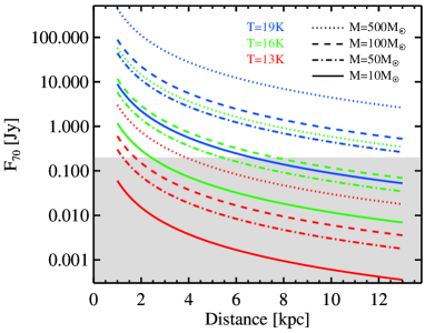
Figure 36: Decrease of the grey-body flux at 70 $\mu$m (Equation 4) for a set of masses and temperatures (dust opacity parameters are those used in this paper), as a function of heliocentric distance. The correspondence between the three probed temperatures and line colours, and the one between the four probed masses and the line style are shown in the legends in the upper part of the plot. The grey shaded area, bordered on the top on the assumed PACS sensitivity limit of 0.2 Jy at 70 $\mu$m, corresponds to the condition in which the grey body source is not expected to be detected with Herschel in Hi-GAL. Considering, for example, a real proto-stellar source emitting a flux 10 times larger than the one expected from the grey body which best fits the SED at $\lambda\geq 160~{}\mu$m, the curves plotted for 100 and $500~{}M_{\odot}$ would assume in this case the role of those plotted for 10 and $50~{}M_{\odot}$, respectively, to assess the detectabilityof such source.

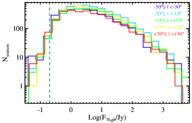
Figure 37: Distributions of 70 $\mu$m fluxes used in this paper, obtained separately over Galactic longitude bins of width $20^{\circ}$ (the bins are reported at the top right of the plot, together with the bin-colour correspondence.). The assumed PACS sensitivity limit of 0.2 Jy at 70 $\mu$m is reported as a vertical grey dashed line.

As already mentioned in Section 3.5, the confusion effect discussed above is in competition with the possible inability of detecting emission at 70 $\mu$m from distant and relatively small proto-stellar clumps, leading to their misclassification as starless sources. In Figure 36 we propose a simple exercise to show how the grey-body flux at 70 $\mu$m, obtained with Equation 4 exploring a grid of values of mass and temperature and using the same dust parameters reported in Section 4, decreases as a function of source heliocentric distance. We compare these trends with the typical PACS sensitivity limit at this band found in our catalogue, which mildly depends on the line of sight and we assume to be 0.2 Jy, as indicated by Figure 34. To better investigate a possible dependence of this limit on the Galactic longitude (although Molinari et al., 2016a, have already shown that the PACS 70 $\mu$m band is the least affected by this effect among the Herschel bands) in Figure 37 we plot the distributions of the 70 $\mu$m fluxes used in this paper, built for five $20^{\circ}$-wide different chunks of longitude. For all the five histograms, the bin containing the 0.2 Jy flux is the smallest containing a statistically significant ($N>10$) number of sources. With respect to this value, in Figure 36 one sees that a grey body with $M\leq 50~{}M_{\odot}$ and $T\leq 16~{}$K could not be detected at $d\gtrsim 5$ kpc, while only more favourable parameter combinations (such as, for example, $M\geq 500~{}M_{\odot}$ and $T\geq 16~{}K$, or $M\geq 50~{}M_{\odot}$ and $T>19$ K) can remain detectable up to $d=13$ kpc, a value which is representative of very far objects in our catalogue. Clearly, in the approach followed in this paper, consisting of modeling the portion of the SED at $\lambda\geq 160~{}\mu$m with a grey body and the flux observed at 70 $\mu$m ($F_{\mathrm{70,obs}}$) as a simple upper limit to better constrain the fit, this flux is expected to in excess with respect to the grey body ($F_{\mathrm{70,gb}}$) best-fitting the SED at the longer wavelengths. Obviously, this adds a further degree of freedom, so that, for example, one can review the curves plotted in Figure 36 for the case $M=500~{}M_{\odot}$ as those of a source with $M=50~{}M_{\odot}$ and $F_{\mathrm{70,obs}}/F_{\mathrm{70,gb}}=10$, and so on (we estimate that, for sources present in our catalogue, $F_{\mathrm{70,obs}}/F_{\mathrm{70,gb}}<10$ is found in around half of the cases in which $F_{\mathrm{70,obs}}$ is available). In conclusion, due to the difficulty in describing $F_{\mathrm{70,obs}}$ through a simple model, it is not possible to predict accurately its value starting from the rest of the SED, nevertheless we expect that a minor but significant fraction of relatively low-mass (and/or low-temperature) clumps observed at large distances and flagged as starless sources are actually misclassified due a selection effect un the flux at 70 $\mu$m.

C.2 Mass completeness limits

A discussion of the mass completeness limits for the Hi-GAL sources requires as a first step to identify the most suitable band for estimating masses. Intuitively, wavelengths at which the emission is optically thin so that the integrated flux can be considered proportional to the amount of matter in the clump, should be taken into account. The 500 $\mu$m band might be the preferred one, but according to the constraints stated in Section 3.1, the flux at this band may be not present in all the considered SEDs, while fluxes at 250 and 350 $\mu$m are always present by construction. In Figure 38 we show the relation between the masses of the catalogue sources and their fluxes at these two bands; to remove the dependence on the distance, the masses have been scaled to the same “virtual” distance $d_{v}=1$ kpc, through a factor $(d_{v}/d)^{2}$ (or, for sources having no kinematic distance estimate, imposing their distance to be just $d_{v}$). Of course, from the analytic point of view such relation is expected to depend on the temperature, so that also lines corresponding to grey bodies at different temperatures and $\beta=2$ are overplotted. As expected, the level of spread is smaller (than a tighter correlation is found) in the mass vs $F_{350}$ plot, which we adopt hereafter for the following analysis of the completeness limit.

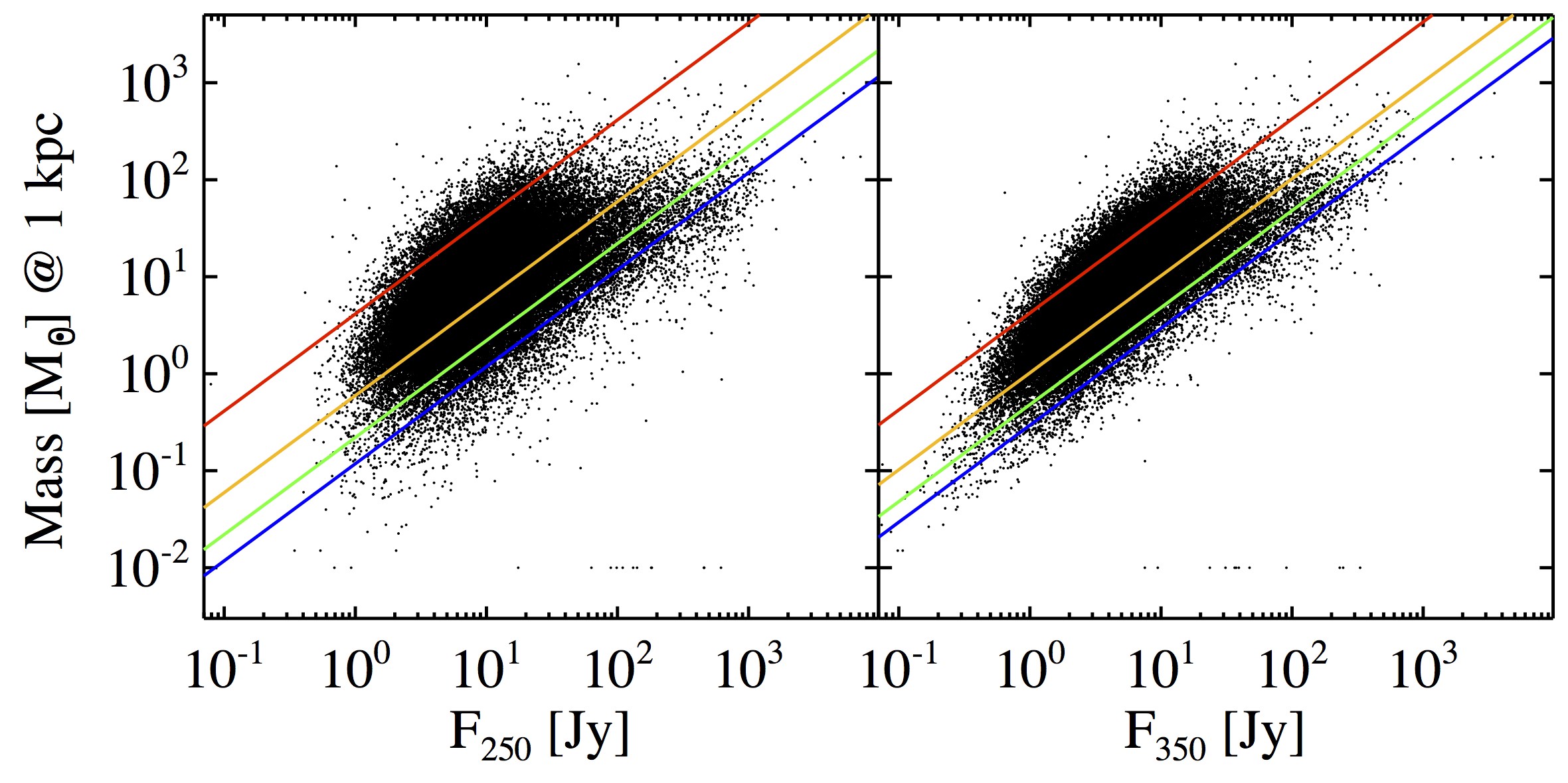
Figure 38: Left: relation grey body mass vs flux at $250~{}\mu$m for all the sources included in the Hi-GAL physical catalogue. The same relation for a grey body is represented with solid lines for four different temperatures: 10 (red), 15 (orange), 20 (green), and 25 K (blue), respectively. Right: the same as in the left panel, but for the flux at $350~{}\mu$m.

Molinari et al. (2016a) provided 90% completeness limits for their photometric catalogues at all the five Hi-GAL bands, subdivided by tile. Thus, given a completeness limit $F{{}_{\mathrm{compl,350}}}$ at 350 $\mu$m (as a function of the considered tile, so, roughly, of the Galactic longitude), the 90% mass completeness limit will depend on the source temperature (according to the grey body law) and on its distance (being $M_{\mathrm{compl}}$ proportional to $d^{2}$). Collapsing all the involved constants and unit conversion factors, such dependency can be condensed as

$$\frac{M_{\mathrm{compl}}(T,d)}{\mathrm{M_{\odot}}}=0.0705\>\left(\frac{F{{}_{\mathrm{compl,350}}}}{\mathrm{Jy}}\right)\>\left(\frac{d}{\mathrm{kpc}}\right)^{2}\>\left(\exp{\left(\frac{41.1094}{\left(T/\mathrm{K}\right)}\right)-1}\right)\;.$$ (7)

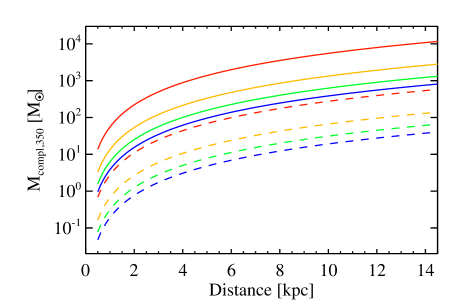
Figure 39: Curves of the 90% mass completeness limit based on the photometry at 350 $\mu$m, as a function of the source distance, according to Equation 7. Two values of $F{{}_{\mathrm{compl,350}}}$ are probed (see text): solid and dashed curves correspond, to 13.08 and 0.65 Jy, respectively. Finally, four values of the temperature parameters are probed, namely the same as in Figure 38, represented using the same colour encoding.

In Figure 39, the behaviour of the mass completeness limit based on Equation 7 is reported, showing how it varies as a function of the distance for two values of $F{{}_{\mathrm{compl,350}}}$, namely the maximum and the minimum ones found by Molinari et al. (2016a) in their Hi-GAL completeness analysis (13.08 and 0.65 Jy, respectively), and for four temperatures between 10 and 25 K. Using the Hi-GAL physical catalogue, therefore, will require to take into account such mass completeness limits.

Appendix D Clump property consistency with respect to previous surveys

A blind comparison between our clump property catalogue with the results of previous surveys of the Galactic ISM can turn out to be misleading if no attention is paid to the assumptions such catalogues are built on. The main one is the definition itself of the source typology, in turn depending on the characteristics of the exploited observations (wavelength domain, tracer, resolution, sensitivity, etc.).

We reaffirm here that this paper deals with the properties of Herschel compact sources (i.e. with an angular extent no larger than a few tens of arcsecs) whose SEDs are eligible for modified black body fit at $\lambda\geq 160~{}\mu$m. Depending on the distance, these sources can correspond to pre- or proto-stellar cores, or (in the most likely case) to larger clumps, or even to entire clouds (Section 6.1). The wavelength range we consider for the grey-body fit allows us to obtain global/average properties of the cold envelope component of the sources. Instead, for obtaining the bolometric luminosity we consider also fluxes at shorter wavelengths, to take into account the emission from the possible proto-stellar content of the Hi-GAL source. We finally recall that, through appropriate assumptions and operations (flux scaling), we estimate the source properties as referred to a volume corresponding to the deconvolved source size observed at $250~{}\mu$m.

An interesting comparison can be carried out with the data coming from the Census of High- and Medium-mass Protostars (CHaMP) survey (Barnes et al., 2011; Ma et al., 2013). The 303 CHaMP sources were identified in HCO⁺(1-0) Mopra observations in the coordinate range $280^{\circ}<\ell<300^{\circ}$, $-4^{\circ}<b<2^{\circ}$ (Barnes et al., 2011). Masses were estimated from HCO⁺(1-0), while collecting MSX, IRAS, and SIMBA-SEST photometry SEDs were built to estimate the bolometric luminosity and, at $\lambda\geq 60~{}\mu$m, the temperature of the cold envelope (Ma et al., 2013).

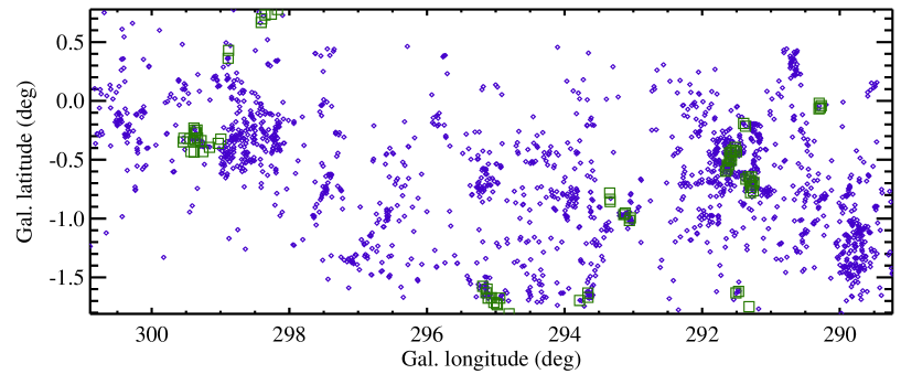
Figure 40: Spatial dispposition of Hi-GAL proto-stellar sources (blue diamonds) and CHaMP ones (green squares), respectively, in the common surveyed area.

The most striking difference between the CHaMP and Hi-GAL source global behaviour lies in the statistics of $L_{\mathrm{bol}}/M$ (Ma et al., 2013, their Figure 2, $d$, and our Figure 13, respectively). In their case, $L_{\mathrm{bol}}/M$ distribution peaks at few tens $L_{\odot}/M_{\odot}$, while in our case, for the proto-stellar population, the peak position is found to be smaller of about one order of magnitude. To check this discrepancy, we searched for the Hi-GAL proto-stellar sources having a positional match with the ones of the CHaMP catalogue. In the common surveyed area, we found 6513 and 77 sources for Hi-GAL and CHaMP, respectively, with 69 matches within a searching radius of $2\arcmin$. Cases of multiple associations were resolved keeping only the Hi-GAL closest counterpart of each CHaMP source. In this way, distance-independent quantities such as $T$ and $L_{\mathrm{bol}}/M$ can be directly compared. Instead $M$ and $L_{\mathrm{bol}}$ depend on the distance adopted in the two different surveys, so that the best way to compare them is to rescale these quantities to report them to the same virtual distance $d_{v}$, similarly to the procedure adopted in the previous section.

Figure 41: Comparison of physical properties derived for Hi-GAL and CHaMP compact sources. Top, left: comparison of masses for sources found in both surveys; masses are scaled to a common distance of 1 kpc to allow unbiased comparison. Top, right: the same as in the previous panel, but for bolometric luminosities. Bottom, left: comparison of $L_{\mathrm{bol}}/M$ ratios (distance-independent) for the sources of the two previous panels. Bottom, right: the same as in the previous panel, but for temperatures. In all panels the bisector corresponding to the 1:1 relation is represented as a dotted line.

Figures 40 and 41 illustrate a comparison of the two surveys, in the overlap area. In the former, the angular disposition of the sources is shown, while in the latter masses and luminosities, scaled at $d_{v}=1$ kpc, are compared (top left and right panels, respectively). Both quantities show a wide spread around the 1:1 relation. While masses were determined using different methods, the differences in luminosity can be deduced from the different way the SEDs were built: on the one hand CHaMP uses IRAS fluxes, which are expected to come from an area in the sky remarkably larger than that of the typical Hi-GAL sources (so the resulting luminosity tends to be significantly larger), on the other hand such CHaMP SEDs do not cover the crucial range $100-500~{}\mu$m in which emission from cold dust peaks, thus potentially neglecting part of the clump FIR luminosity. The first effect seems to be prevailing in the majority of cases, being the median of the $L_{\mathrm{bol,CH}}/L_{\mathrm{bol,HG}}\sim 16$. Furthermore, since the FIR portion of the CHaMP SEDs generally peaks at shorter wavelengths than Hi-GAL SEDs, also the envelope temperatures are systematically found to be higher in the former case, as clearly shown in the right lower panel of Figure 41. All these contributions lead to shift the CHaMP distribution of $L_{\mathrm{bol}}/M$ compared with Hi-GAL (left lower panel), so that the median value for the ratio between $L_{\mathrm{bol}}/M$ of CHaMP and Hi-GAL is $\sim 4$.

A more direct comparison can be carried out with first results of the Herschel key-program The Earliest Phases of Star formation (EPoS, Ragan et al., 2012). This program consisted in a PACS and SPIRE photometric mapping survey of objects known to be in the cold early phases of star formation. 60 targets were observed, 45 of which corresponding to high-mass star forming regions, in which Ragan et al. (2012) found 496 compact sources. Out of these, 90 lie in the portion of the Galactic plane considered in this paper, (43 in the first quadrant and 47 in the fourth one, Figure 42 $a$ and $b$, respectively). The sources were detected only in PACS images at 70, 100, and 160 $\mu$m, respectively. SPIRE maps were not used either for detecting counterparts or, even more so, for extracting photometry at these wavelengths. This prevents an exact match between the 90 EPoS objects and the entries of our Hi-GAL physical catalogue: first, in several cases clusters of PACS EPoS sources might correspond to a single SPIRE counterpart due to different resolution and, second, possible Hi-GAL equivalents of EPoS sources might not survive the selection process described in 3.1 and based on SED regularity between 160 and 500 $\mu$m. In the end, we found 50 matches between the list of Ragan et al. (2012) and our Hi-GAL physical catalogue, within a searching radius of 1$\arcmin$.

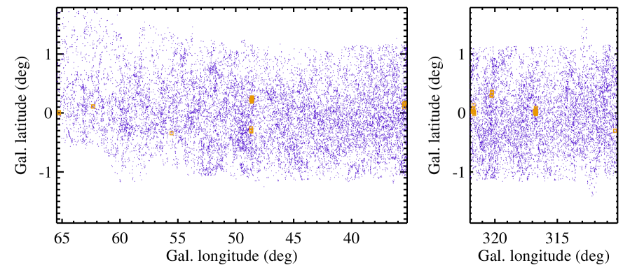
Figure 42: Spatial disposition of Hi-GAL (blue dots) and EPoS (gold squares) sources, respectively, in the common surveyed areas in the first (left) and the fourth (right) Galactic quadrant, respectively.

For these sources, the fluxes at 70 and 160 $\mu$m can be directly compared, (Figure 43, left and right, respectively). In both cases, the Hi-GAL ones appear generally overestimated with respect to the EPoS ones. The most general reason of this discrepancy has to be searched in the different way the fluxes were extracted in the two cases. Ragan et al. (2012) carried out PSF photometry, implicitly assuming a point-like appearance of the sources, while in this work compact sources were extracted with CuTEx, thus considering that source sizes can extend up to a few PSFs and consequently measuring larger total fluxes over larger areas. This aspect is emphasised in Figure 43, using different colours for denoting the different source sizes of the Hi-GAL sources; as a general trend the photometric data of the two surveys depart from equality as the source size estimates in Hi-GAL depart from the PSF extent.

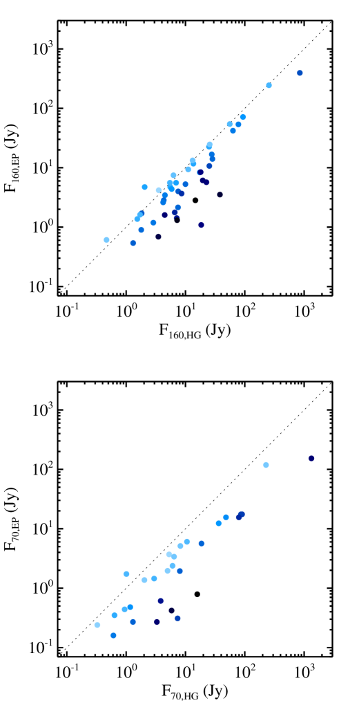
Figure 43: Comparison of EPoS vs Hi-GAL integrated fluxes at 70 (left) and 160 $\mu$m (right), respectively. Different shades of blue are used to represent the size of the Hi-GAL source (estimated as the average FWHM of 2-D Gaussian resulting from the fit performed by CuTEX), to highlight that larger flux discrepancies correspond to larger estimates of the Hi-GAL source sizes: the lightest blue level corresponds to the smallest sizes found at 70 and 160 $\mu$m (9$\arcsec$ and 12.4$\arcsec$, respectively), while black correspond to the largest sizes (23.7$\arcsec$ and 40.8$\arcsec$, respectively).

Photometric discrepancies are among possible explanations of further differences found comparing physical properties of the two source lists, analyzed in Figure 44. EPoS source temperatures are found to be overestimated compared with those in Hi-GAL (top left panel). This is expected due to the different wavelength range explored and considered for the grey body fit, being the latter more suited to trace the peak of the cold dust (see a similar discussion in Fontani et al., 2005). This is also the main reason of generally finding lower mass estimates in EPoS than in Hi-GAL (after rescaling both at a virtual distance $d_{v}=1$ kpc), as shown in Figure 44, top right panel: as a general trend, the larger is the temperature discrepancy, the larger is consequently the mass discrepancy. EPoS bolometric luminosities are generally smaller than Hi-GAL ones (bottom left panel), being the median ratio of the two equal to $\sim 0.26$. This is due to the wider spectral coverage of the SEDs in this paper, potentially going from 21 $\mu$m to 1.1 mm, and also to the lower fluxes measured in EPoS at 70 and 160 $\mu$m, as described above. Finally, combining the information contained in the two previous panels, in the bottom right panel we show the comparison of the $L_{\mathrm{bol}}/M$ ratio for the two surveys: this ratio is generally larger for EPoS despite the larger luminosities found in Hi-GAL since masses at the denominator overcompensate for that. Furthermore, largest discrepancies correspond to largest temperature discrepancies.

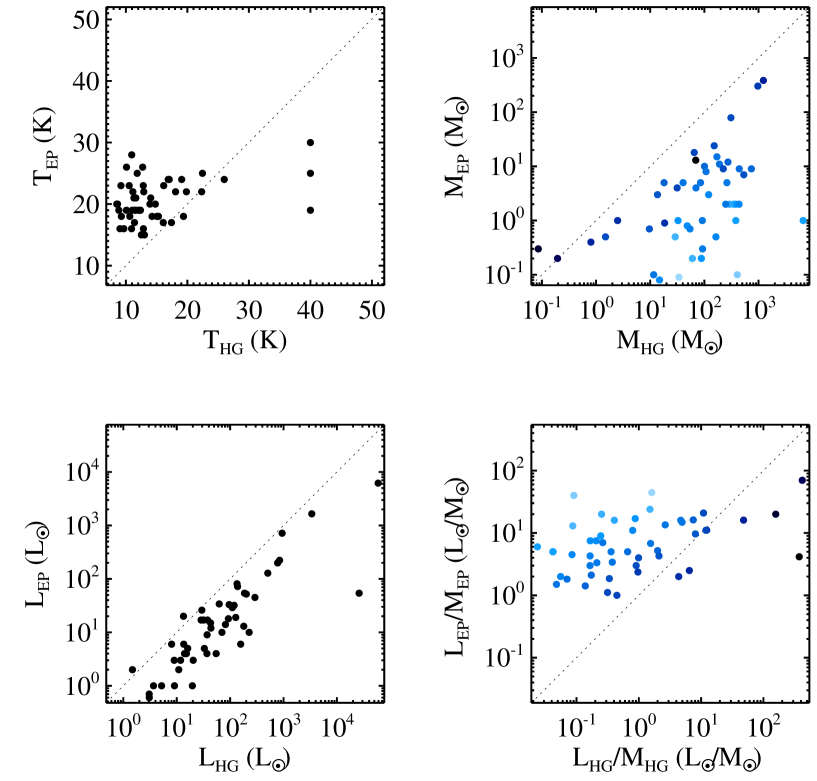
Figure 44: Comparison of physical properties derived for Hi-GAL and EPoS (Ragan et al., 2012) compact sources. Top, left: comparison of temperatures for sources found in both surveys. Top, right: the same as in the previous panel, but for masses scaled to a common virtual distance of 1 kpc to allow unbiased comparison. Different shades of blue are used for the symbols to represent the $\Delta T=T_{\mathrm{HG}}-T_{\mathrm{EP}}$ temperature discrepancy between Hi-GAL and EPoS for each source, going from 21 K (black) to -17 K (light blue). Bottom, left: The same as in top left panel, but for bolometric luminosities scaled to a common virtual distance of 1 kpc. Bottom, right: comparison of $L_{\mathrm{bol}}/M$ ratios for the sources of the previous panels. Different shades of blue are used as in the top right panel. Finally, in all panels the bisector corresponding to the 1:1 relation is represented as a dotted line.

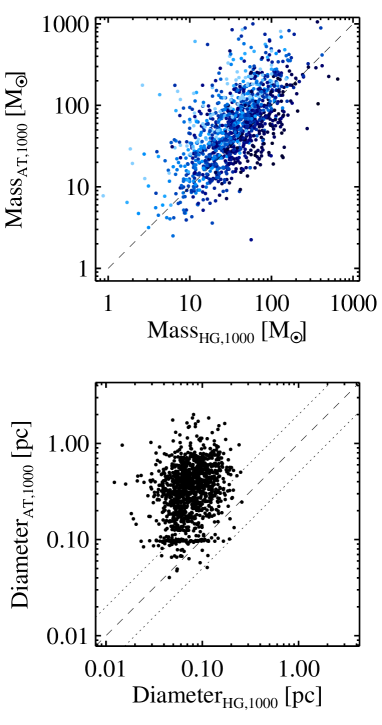
Figure 45: Comparison of physical properties derived for Hi-GAL and ATLASGAL (Wienen et al., 2015) compact sources, re-scaled to a common virtual distance $d_{v}=1$ kpc. Top: comparison of masses for sources found in both surveys. Different shades of blue are used for the symbols to represent the Hi-GAL temperature going from 5 K (black) to 30 K (light blue). The grey dashed line represents the 1:1 relation. Bottom: comparison of diameters, re-scaled to $d_{v}$. The grey dashed line represents the 1:1 relation, while the dotted lines correspond to the ratios 2 and 0.5, respectively.

The above comparison shows that both the considered spectral range and adopted photometry strategy can lead to quite different interpretation of the physical and evolutionary status of the same source. This must be kept in mind in discussing the results presented in this paper as well as in comparing the present Hi-GAL catalogue with other catalogues of similar sources. Particular care, for instance, has to be taken comparing Hi-GAL clump properties with those derived for two single-band sub-millimetre surveys, namely ATLASGAL and BGPS, whose data have been also used in this work. Starting with the former, we compare Hi-GAL clump masses derived in this work with those derived using only the ATLASGAL flux at 870 $\mu$m (Wienen et al., 2015) Notice that in this last work the masses are based on the fluxes of Contreras et al. (2013) and Urquhart et al. (2014b) typically much larger than those in the catalogue of Csengeri et al. (2014), due to different estimate of the source size. As a consequence of this, we could not establish an immediate association between Hi-GAL and ATLASGAL sources of Wienen et al. (2015) simply exploiting the ATLASGAL counterparts already quoted in our catalogue (which instead are taken from Csengeri et al., 2014), but we had to search for positional matching within a searching radius of 36″, i.e. the centroid position accuracy provided by Wienen et al. (2015). In Figure 45, top panel, the comparison of masses is shown; to make it meaningful, the masses of both lists have been re-scaled to a virtual distance of 1 kpc, as also done in the previous comparisons with other surveys. Two main aspects are evident in the plot: $i$) a certain degree of spread around a linear relation is present, mostly due to the spread in Hi-GAL temperature, as opposed to the fact that masses of Wienen et al. (2015) are obtained for a fixed temperature (namely 23.1 and 20.8 K for the fourth and the first Galactic quadrant, respectively), as highlighted by the colour scale adopted to represent the Hi-GAL temperature; $ii$) a remarkable departure of this trend from a 1:1 behaviour, in which the masses of Wienen et al. (2015) are larger than the Hi-GAL ones. This is essentially related to the aforementioned discrepancy between source sizes. In Figure 45, bottom panel, it can be seen how re-scaled diameters (or, equivalently, angular sizes) of sources determined by Wienen et al. (2015) are systematically and significantly larger than those observed for Hi-GAL sources, so that the fluxes (and, correspondingly the masses) are evaluated over larger areas of the sky.

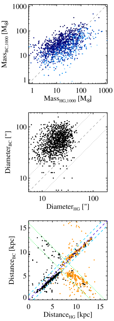
Figure 46: Top, centre: the same as top and bottom panels of Figure 45, respectively, but for BGPS sources (Svoboda et al., 2016). In the top panel angular beam-deconvolved diameters are compared, instead of linear sizes, this information being directly available in the catalogue of Svoboda et al. (2016). Bottom: Comparison of heliocentric BGPS and Hi-GAL distances: black dots are sources for which the far/near Hi-GAL distance ambiguity has been fully solved in this work, orange dots for the less reliable cases in which the far distance has been assumed as final decision due to lack of other indicators. The bisector corresponding to the 1:1 relation is represented as a dark blue dashed line; two further light blue dashed lines are plotted 1 kpc above and beolow it, respectively. Two green dotted lines represent the region populated by sources for which the near/far distance ambiguity has been solved in opposite ways in the two catalogues.

In a similar way it is possible to make a comparison of masses derived in this paper and those of of a sample of massive BGPS sources studied in Svoboda et al. (2016). In this case, the BGPS source designation used is the same as in the BGPS catalogue (i.e. Ginsburg et al., 2013). Similarly to the ATLASGAL case, the majority of BGPS masses appear in excess compared to Hi-GAL (Figure 46, top), typically as a consequence of a larger angular size assigned to the source (Figure 46, center). Again, the spread in mass differences appears mostly due to the spread of Hi-GAL source grey body temperatures.

This comparative analysis with BGPS parameters offers us the opportunity of testing the heliocentric distances used in our catalogue ($d_{\mathrm{HG}}$). The comparison with BGPS distances ($d_{\mathrm{BC}}$), derived by Ellsworth-Bowers et al. (2013, 2015), is shown in the bottom panel of Figure 46. A significant number of points is located close to the bisector (459 within $\lvert d_{\mathrm{BC}}-d_{\mathrm{HG}}\rvert<1$ kpc, out of 816 plotted points), demonstrating a good agreement between the two methods in these cases. Using a different colour for sources of our catalogue for which the near/far distance ambiguity is not solved (so that the far distance is chosen by default and a bad quality flag is assigned, see Section 3.4), it can be seen that in several cases the validity of such choice is supported by a good agreement with a BGPS distance. Departures from the 1:1 behaviour, following peculiar trends (e.g. the one at 5 kpc$\lesssim d_{\mathrm{HG}}\lesssim$ 7 kpc) are ascribable to different Galactic rotation models adopted. Another trend is clearly visible along the “orthogonal” direction, easily explainable with cases in which the near distance estimate has been assigned in one of the two catalogues, and the far distance in the other. This trend is not as tight as the one around the bisector: delimiting by eye the region populated by sources following this trend (see figure), and neglecting the area corresponding to the intersection with the $\pm 1$ kpc-belt around the bisector, we find 226 sources characterised by this discrepancy. Noticeably, in the lower part of this area, corresponding to sources with an assigned far distance in our catalogue, such assignment is flagged in most cases as “bad quality”. Finally, a total of 131 sources (i.e. the 16% of the sources considered for this test) remain out of these two main trends, and correspond to distances that can not be reconciled simply changing the near/far decision.

Author afilliations
¹INAF-IAPS, via del Fosso del Cavaliere 100, 00133 Roma, Italy
²Space Telescope Science Institute, 3700 San Martin Dr., Baltimore, MD, 21218, USA
³Astrophysics Research Institute, Liverpool John Moores University, Liverpool Science Park Ic2, 146 Brownlow Hill, Liverpool, L3 5RF, UK
⁴Aix Marseille Univ., CNRS, LAM, Laboratoire d’Astrophysique de Marseille, Marseille, France
⁵Max-Planck Institute for Astronomy, Königstuhl 17, D-69117 Heidelberg, Germany
⁶Infrared Processing Analysis Center, California Institute of Technology, 770 South Wilson Ave., Pasadena, CA 91125, USA
⁷Dipartimento di Matematica e Fisica, Università del Salento, 73100, Lecce, Italy
⁸CNRS, IRAP, 9 Av. colonel Roche, BP 44346, F-31028 Toulouse cedex 4, France
⁹Université de Toulouse, UPS-OMP, IRAP, F-31028 Toulouse cedex 4, France
¹⁰Department of Physics, Nagoya University, Chikusa-ku, Nagoya, Aichi 464-8601, Japan
¹¹Department of Physics & Astronomy, University of Calgary, AB, T2N 1N4, Canada
¹²Center for Astrophysics and Space Astronomy, University of Colorado, Boulder, CO, 80309, USA
¹³Canadian Institute for Theoretical Astrophysics, University of Toronto, McLennan Physical Laboratories, 60 St. George Street, Toronto, Ontario, Canada
¹⁴School of Physics and Astronomy, University of Leeds, Leeds LS2 9JT, UK
¹⁵School of Physics and Astronomy, Cardiff University, Cardiff CF24 3AA, Wales, UK
¹⁶IPAG, University Grenoble Alpes, 38000, Grenoble, France
¹⁷AIM Paris-Saclay, CEA/IRFU - CNRS/INSU - Univ. Paris Diderot, Service d’Astrophysique, CEA-Saclay, 91191 Gif-sur-Yvette Cedex, France
¹⁸INAF, Osservatorio Astrofisico di Arcetri, Largo E. Fermi 5, 50125, Firenze, Italy
¹⁹I. Physik. Institut, University of Cologne, Zülpicher Strasse, 50937, Köln, Germany
²⁰European Southern Observatory, Karl Schwarzschild str. 2, 85748, Garching, Germany
²¹Max-Planck-Institut für Radioastronomie, Auf dem Hügel 69, 53121 Bonn, Germany
²²ASI Science Data centre, 00044 Frascati, Roma, Italy
²³ESA/ESAC, PO Box 78, Villanueva de la Cañada, 28691, Madrid, Spain
²⁴Dipartimento di Fisica e Scienze della Terra, Università degli Studi di Ferrara e Sezione INFN di Ferrara, via Saragat 1, 44100, Ferrara, Italy
²⁵Instituto de Astrofísica e Ciências do Espaço, Universidade do Porto, CAUP, Rua das Estrelas, PT4150-762 Porto, Portugal
²⁶Dipartimento di Fisica, Università di Roma “La Sapienza”, P.le Aldo Moro 2, 00138, Roma, Italy
²⁷DIET, Università di Roma “La Sapienza”, 00185, Roma, Italy
²⁸ESA, Directorate of Science, Science Support Office, ESTEC/SCI-S, Keplerlaan 1, NL-2201 AZ Noordwijk, The Netherlands
²⁹Departamento de Fisica, Universidad de Atacama, Copayapu 485, Copiapó, Chile
³¹Observatoire Astronomique de Strasbourg, Université de Strasbourg, CNRS, UMR 7550, 11 rue de l’Université, 67000, Strasbourg, France
³⁰Observatoire de l’Université de Genève, 51 chemin des Maillettes, 1290, Sauverny, Switzerland
³²CAS Key Laboratory of Space Astronomy and Technology, National Astronomical Observatories, Chinese Academy of Sciences, Beijing 100012, China
³³Département de physique, de génie physique et d’optique and Centre de recherche en Astrophysique du Québec, Université Laval, 1045 avenue de la médecine, Québec, G1V 0A6, Canada
³⁴Italian ALMA Regional Centre, INAF-IRA, Via P. Gobetti 101, 40129 Bologna, Italy
³⁵Centre for Astrophysics Research, School of Physics Astronomy & Mathematics, University of Hertfordshire, College Lane, Hatfield, AL10 9AB, UK
³⁶INAF - Astrophysical Observatory of Catania, Via Santa Sofia 78, 95123, Catania, Italy
³⁷Jeremiah Horrocks Institute, University of Central Lancashire, Preston PR1 2HE, UK
³⁸CERN, 385 Route de Meyrin, 1217 Meyrin, Switzerland
³⁹INAF - Astronomical Observatory of Capodimonte, via Moiariello 16, I-80131 Napoli, Italy
⁴⁰INAF - Osservatorio Astronomico di Trieste, via G.B. Tiepolo 11, Trieste, Italy
⁴¹Department of Physics “E.Pancini”, University Federico II, via Cinthia 6, I-80126 Napoli, Italy
⁴²Institute for Computer Science and Control (MTA SZTAKI), Laboratory of Parallel and Distributed Systems, Victor Hugo u. 18-22., Budapest 1132, Hungary
⁴³Department of Physics and Astronomy, University College London, London, WC1E 6BT, UK
⁴⁴STFC, Rutherford Appleton Labs, Didcot, OX11QX, UK
⁴⁵Nobeyama Radio Observatory, 462-2 Nobeyama Minamimaki-mura, Minamisaku-gun, Nagano 384-1305, Japan

References

- Aguirre et al. (2011) Aguirre J. E., et al., 2011, ApJS, 192, 4
- Ali et al. (2010) Ali B., et al., 2010, A&A, 518, L119
- Andre et al. (1993) Andre P., Ward-Thompson D., Barsony M., 1993, ApJ, 406, 122
- André et al. (2000) André P., Ward-Thompson D., Barsony M., 2000, Protostars and Planets IV, p. 59
- André et al. (2008) André P., et al., 2008, A&A, 490, L27
- André et al. (2010) André P., et al., 2010, A&A, 518, L102
- Avedisova (2000) Avedisova V., 2000, Baltic Astronomy, 9, 569
- Baldeschi et al. (2017) Baldeschi A., et al., 2017, MNRAS, 466, 3682
- Bally & Zinnecker (2005) Bally J., Zinnecker H., 2005, AJ, 129, 2281
- Bally et al. (2010) Bally J., et al., 2010, A&A, 518, L90
- Barnes et al. (2011) Barnes P. J., et al., 2011, ApJS, 196, 12
- Battersby et al. (2010) Battersby C., Bally J., Jackson J. M., Ginsburg A., Shirley Y. L., Schlingman W., Glenn J., 2010, ApJ, 721, 222
- Battersby et al. (2011) Battersby C., et al., 2011, A&A, 535, A128
- Beckwith et al. (1990) Beckwith S. V. W., Sargent A. I., Chini R. S., Guesten R., 1990, AJ, 99, 924
- Beltrán et al. (2013) Beltrán M. T., et al., 2013, A&A, 552, A123
- Bergin & Tafalla (2007) Bergin E. A., Tafalla M., 2007, ARA&A, 45, 339
- Beuther et al. (2010) Beuther H., Henning T., Linz H., Krause O., Nielbock M., Steinacker J., 2010, A&A, 518, L78
- Beuther et al. (2011) Beuther H., Kainulainen J., Henning T., Plume R., Heitsch F., 2011, A&A, 533, A17
- Billot et al. (2011) Billot N., et al., 2011, ApJ, 735, 28
- Bontemps et al. (2010) Bontemps S., et al., 2010, A&A, 518, L85
- Brand & Blitz (1993) Brand J., Blitz L., 1993, A&A, 275, 67
- Bronfman et al. (1996) Bronfman L., Nyman L.-A., May J., 1996, A&AS, 115, 81
- Bronfman et al. (2000) Bronfman L., Casassus S., May J., Nyman L.-Å., 2000, A&A, 358, 521
- Butler & Tan (2012) Butler M. J., Tan J. C., 2012, ApJ, 754, 5
- Carey et al. (2008) Carey S. J., Mizuno D. R., Kraemer K. E., Shenoy S., Noriega-Crespo A., Price S. D., Paladini R., Kuchar T. A., 2008, MIPSGAL v3.0 Data Delivery Description Document (29 August 2008)
- Carey et al. (2009) Carey S. J., et al., 2009, PASP, 121, 76
- Cesaroni et al. (2015) Cesaroni R., et al., 2015, A&A, 579, A71
- Chabrier (2003) Chabrier G., 2003, PASP, 115, 763
- Chen et al. (1995) Chen H., Myers P. C., Ladd E. F., Wood D. O. S., 1995, ApJ, 445, 377
- Churchwell et al. (2009) Churchwell E., et al., 2009, PASP, 121, 213
- Contreras et al. (2013) Contreras Y., et al., 2013, A&A, 549, A45
- Csengeri et al. (2014) Csengeri T., et al., 2014, A&A, 565, A75
- Deharveng et al. (2012) Deharveng L., et al., 2012, A&A, 546, A74
- Dobbs & Bonnell (2007) Dobbs C. L., Bonnell I. A., 2007, MNRAS, 376, 1747
- Draine & Li (2007) Draine B. T., Li A., 2007, ApJ, 657, 810
- Dunham et al. (2008) Dunham M. M., Crapsi A., Evans II N. J., Bourke T. L., Huard T. L., Myers P. C., Kauffmann J., 2008, ApJS, 179, 249
- Dunham et al. (2014) Dunham M. M., et al., 2014, Protostars and Planets VI, pp 195–218
- Eden et al. (2012) Eden D. J., Moore T. J. T., Plume R., Morgan L. K., 2012, MNRAS, 422, 3178
- Eden et al. (2013) Eden D. J., Moore T. J. T., Morgan L. K., Thompson M. A., Urquhart J. S., 2013, MNRAS, 431, 1587
- Eden et al. (2015) Eden D. J., Moore T. J. T., Urquhart J. S., Elia D., Plume R., Rigby A. J., Thompson M. A., 2015, MNRAS, 452, 289
- Egan et al. (1998) Egan M. P., Shipman R. F., Price S. D., Carey S. J., Clark F. O., Cohen M., 1998, ApJ, 494, L199
- Egan et al. (2003) Egan M. P., et al., 2003, VizieR Online Data Catalog, 5114, 0
- Elia & Pezzuto (2016) Elia D., Pezzuto S., 2016, MNRAS, 461, 1328
- Elia et al. (2010) Elia D., et al., 2010, A&A, 518, L97
- Elia et al. (2013) Elia D., et al., 2013, ApJ, 772, 45
- Elia et al. (2014) Elia D., et al., 2014, ApJ, 788, 3
- Ellsworth-Bowers et al. (2013) Ellsworth-Bowers T. P., et al., 2013, ApJ, 770, 39
- Ellsworth-Bowers et al. (2015) Ellsworth-Bowers T. P., Rosolowsky E., Glenn J., Ginsburg A., Evans II N. J., Battersby C., Shirley Y. L., Svoboda B., 2015, ApJ, 799, 29
- Enoch et al. (2008) Enoch M. L., Evans II N. J., Sargent A. I., Glenn J., Rosolowsky E., Myers P., 2008, ApJ, 684, 1240
- Fallscheer et al. (2013) Fallscheer C., et al., 2013, ApJ, 773, 102
- Ferrière (2001) Ferrière K. M., 2001, Reviews of Modern Physics, 73, 1031
- Fish et al. (2003) Fish V. L., Reid M. J., Wilner D. J., Churchwell E., 2003, ApJ, 587, 701
- Fontani et al. (2005) Fontani F., Beltrán M. T., Brand J., Cesaroni R., Testi L., Molinari S., Walmsley C. M., 2005, A&A, 432, 921
- García et al. (2014) García P., Bronfman L., Nyman L.-Å., Dame T. M., Luna A., 2014, ApJS, 212, 2
- Giannetti et al. (2013) Giannetti A., et al., 2013, A&A, 556, A16
- Giannini et al. (2012) Giannini T., et al., 2012, A&A, 539, A156
- Ginsburg et al. (2012) Ginsburg A., Bressert E., Bally J., Battersby C., 2012, ApJ, 758, L29
- Ginsburg et al. (2013) Ginsburg A., et al., 2013, ApJS, 208, 14
- Green & McClure-Griffiths (2011) Green J. A., McClure-Griffiths N. M., 2011, MNRAS, 417, 2500
- Griffin et al. (2010) Griffin M. J., et al., 2010, A&A, 518, L3
- Gutermuth & Heyer (2015) Gutermuth R. A., Heyer M., 2015, AJ, 149, 64
- Guzmán et al. (2015) Guzmán A. E., Sanhueza P., Contreras Y., Smith H. A., Jackson J. M., Hoq S., Rathborne J. M., 2015, ApJ, 815, 130
- Hatchell & Fuller (2008) Hatchell J., Fuller G. A., 2008, A&A, 482, 855
- He et al. (2015) He Y.-X., et al., 2015, MNRAS, 450, 1926
- Hoare et al. (2012) Hoare M. G., et al., 2012, PASP, 124, 939
- Hofner et al. (2000) Hofner P., Wyrowski F., Walmsley C. M., Churchwell E., 2000, ApJ, 536, 393
- Hou et al. (2009) Hou L. G., Han J. L., Shi W. B., 2009, A&A, 499, 473
- Jackson et al. (2006) Jackson J. M., et al., 2006, ApJS, 163, 145
- Kainulainen et al. (2009) Kainulainen J., Beuther H., Henning T., Plume R., 2009, A&A, 508, L35
- Kato et al. (1999) Kato S., Mizuno N., Asayama S.-i., Mizuno A., Ogawa H., Fukui Y., 1999, PASJ, 51, 883
- Kauffmann & Pillai (2010) Kauffmann J., Pillai T., 2010, ApJ, 723, L7
- Könyves et al. (2010) Könyves V., et al., 2010, A&A, 518, L106
- Könyves et al. (2015) Könyves V., et al., 2015, A&A, 584, A91
- Krumholz & McKee (2008) Krumholz M. R., McKee C. F., 2008, Nature, 451, 1082
- Lada (1987) Lada C. J., 1987, in Peimbert M., Jugaku J., eds, IAU Symposium Vol. 115, Star Forming Regions. pp 1–17
- Lada & Wilking (1984) Lada C. J., Wilking B. A., 1984, ApJ, 287, 610
- Larson (1981) Larson R. B., 1981, MNRAS, 194, 809
- Lawrence et al. (2007) Lawrence A., et al., 2007, MNRAS, 379, 1599
- Li et al. (2012) Li J. J., et al., 2012, ApJ, 749, 47
- López-Sepulcre et al. (2010) López-Sepulcre A., Cesaroni R., Walmsley C. M., 2010, A&A, 517, A66
- Lumsden et al. (2013) Lumsden S. L., Hoare M. G., Urquhart J. S., Oudmaijer R. D., Davies B., Mottram J. C., Cooper H. D. B., Moore T. J. T., 2013, ApJS, 208, 11
- Ma et al. (2013) Ma B., Tan J. C., Barnes P. J., 2013, ApJ, 779, 79
- Makovoz & Marleau (2005) Makovoz D., Marleau F. R., 2005, PASP, 117, 1113
- Martin et al. (2010) Martin P. G., et al., 2010, A&A, 518, L105
- Martin et al. (2012) Martin P. G., et al., 2012, ApJ, 751, 28
- Maury et al. (2011) Maury A. J., André P., Men’shchikov A., Könyves V., Bontemps S., 2011, A&A, 535, A77
- Merello et al. (2015) Merello M., Evans II N. J., Shirley Y. L., Rosolowsky E., Ginsburg A., Bally J., Battersby C., Dunham M. M., 2015, ApJS, 218, 1
- Molinari et al. (2008) Molinari S., Pezzuto S., Cesaroni R., Brand J., Faustini F., Testi L., 2008, A&A, 481, 345
- Molinari et al. (2010a) Molinari S., et al., 2010a, PASP, 122, 314
- Molinari et al. (2010b) Molinari S., et al., 2010b, A&A, 518, L100
- Molinari et al. (2011) Molinari S., Schisano E., Faustini F., Pestalozzi M., di Giorgio A. M., Liu S., 2011, A&A, 530, A133
- Molinari et al. (2014) Molinari S., et al., 2014, Protostars and Planets VI, pp 125–148
- Molinari et al. (2016a) Molinari S., et al., 2016a, A&A, 591, A149
- Molinari et al. (2016b) Molinari S., Merello M., Elia D., Cesaroni R., Testi L., Robitaille T., 2016b, ApJ, 826, L8
- Molinaro et al. (2016) Molinaro M., et al., 2016, ] 10.1117/12.2231674, 9913, 99130H
- Momany et al. (2006) Momany Y., Zaggia S., Gilmore G., Piotto G., Carraro G., Bedin L. R., de Angeli F., 2006, A&A, 451, 515
- Moore et al. (2015) Moore T. J. T., et al., 2015, MNRAS, 453, 4264
- Motte et al. (2010a) Motte F., et al., 2010a, A&A, 518, L77
- Motte et al. (2010b) Motte F., et al., 2010b, A&A, 518, L77
- Motte et al. (2014) Motte F., et al., 2014, A&A, 571, A32
- Mueller et al. (2002) Mueller K. E., Shirley Y. L., Evans II N. J., Jacobson H. R., 2002, ApJS, 143, 469
- Myers & Ladd (1993) Myers P. C., Ladd E. F., 1993, ApJ, 413, L47
- Myers et al. (1998) Myers P. C., Adams F. C., Chen H., Schaff E., 1998, ApJ, 492, 703
- Netterfield et al. (2009) Netterfield C. B., et al., 2009, ApJ, 707, 1824
- Nguyen Luong et al. (2011) Nguyen Luong Q., et al., 2011, A&A, 529, A41
- Olmi et al. (2009) Olmi L., et al., 2009, ApJ, 707, 1836
- Olmi et al. (2013) Olmi L., et al., 2013, A&A, 551, A111
- Onishi et al. (2005) Onishi T., Mizuno N., Mizuno A., Fukui Y., Nanten Team 2005, in Protostars and Planets V Posters. p. 8301
- Ossenkopf & Henning (1994) Ossenkopf V., Henning T., 1994, A&A, 291, 943
- Paladini et al. (2012) Paladini R., et al., 2012, ApJ, 760, 149
- Pekruhl et al. (2013) Pekruhl S., Preibisch T., Schuller F., Menten K., 2013, A&A, 550, A29
- Peretto & Fuller (2010) Peretto N., Fuller G. A., 2010, ApJ, 723, 555
- Peretto et al. (2010) Peretto N., et al., 2010, A&A, 518, L98
- Persi et al. (2016) Persi P., Tapia M., Roth M., Elia D., López-Vázquez J. A., 2016, MNRAS, 459, 1946
- Pezzuto et al. (2012) Pezzuto S., et al., 2012, A&A, 547, A54
- Piazzo et al. (2012) Piazzo L., Ikhenaode D., Natoli P., Pestalozzi M., Piacentini F., Traficante A., 2012, IEEE Transactions on Image Processing, 21, 3687
- Pilbratt et al. (2010) Pilbratt G. L., et al., 2010, A&A, 518, L1
- Poglitsch et al. (2010) Poglitsch A., et al., 2010, A&A, 518, L2
- Polychroni et al. (2013) Polychroni D., et al., 2013, ApJ, 777, L33
- Preibisch et al. (1993) Preibisch T., Ossenkopf V., Yorke H. W., Henning T., 1993, A&A, 279, 577
- Purcell et al. (2013) Purcell C. R., et al., 2013, ApJS, 205, 1
- Ragan et al. (2009) Ragan S. E., Bergin E. A., Gutermuth R. A., 2009, ApJ, 698, 324
- Ragan et al. (2012) Ragan S., et al., 2012, A&A, 547, A49
- Ragan et al. (2013) Ragan S. E., Henning T., Beuther H., 2013, A&A, 559, A79
- Ragan et al. (2016) Ragan S. E., Moore T. J. T., Eden D. J., Hoare M. G., Elia D., Molinari S., 2016, MNRAS, 462, 3123
- Reid & Wilson (2005) Reid M. A., Wilson C. D., 2005, ApJ, 625, 891
- Reid & Wilson (2006) Reid M. A., Wilson C. D., 2006, ApJ, 644, 990
- Reid et al. (2010) Reid M. A., Wadsley J., Petitclerc N., Sills A., 2010, ApJ, 719, 561
- Rodgers et al. (1960) Rodgers A. W., Campbell C. T., Whiteoak J. B., 1960, MNRAS, 121, 103
- Roman-Duval et al. (2009) Roman-Duval J., Jackson J. M., Heyer M., Johnson A., Rathborne J., Shah R., Simon R., 2009, ApJ, 699, 1153
- Rosolowsky et al. (2010) Rosolowsky E., et al., 2010, ApJS, 188, 123
- Russeil (2003) Russeil D., 2003, A&A, 397, 133
- Russeil et al. (2011) Russeil D., et al., 2011, A&A, 526, A151
- Sadavoy et al. (2013) Sadavoy S. I., et al., 2013, ApJ, 767, 126
- Salpeter (1955) Salpeter E. E., 1955, ApJ, 121, 161
- Saraceno et al. (1996) Saraceno P., Andre P., Ceccarelli C., Griffin M., Molinari S., 1996, A&A, 309, 827
- Schisano et al. (2014) Schisano E., et al., 2014, ApJ, 791, 27
- Schneider et al. (2012) Schneider N., et al., 2012, A&A, 540, L11
- Schuller et al. (2009) Schuller F., et al., 2009, A&A, 504, 415
- Shirley et al. (2003) Shirley Y. L., Evans II N. J., Young K. E., Knez C., Jaffe D. T., 2003, ApJS, 149, 375
- Smith (2014) Smith M. D., 2014, MNRAS, 438, 1051
- Smith et al. (2008) Smith R. J., Clark P. C., Bonnell I. A., 2008, MNRAS, 391, 1091
- Spezzi et al. (2013) Spezzi L., et al., 2013, A&A, 555, A71
- Stetson (1987) Stetson P. B., 1987, PASP, 99, 191
- Stil et al. (2006) Stil J. M., et al., 2006, AJ, 132, 1158
- Strafella et al. (2010) Strafella F., et al., 2010, ApJ, 719, 9
- Strafella et al. (2015) Strafella F., et al., 2015, ApJ, 798, 104
- Stutzki et al. (1998) Stutzki J., Bensch F., Heithausen A., Ossenkopf V., Zielinsky M., 1998, A&A, 336, 697
- Svoboda et al. (2016) Svoboda B. E., et al., 2016, ApJ, 822, 59
- Tackenberg et al. (2012) Tackenberg J., et al., 2012, A&A, 540, A113
- Tan (2005) Tan J. C., 2005, in Kumar M. S. N., Tafalla M., Caselli P., eds, Cores to Clusters: Star Formation with Next Generation Telescopes. p. 87 (arXiv:astro-ph/0504256)
- Tapia et al. (2014) Tapia M., Persi P., Roth M., Elia D., Molinari S., Saldaño H. P., Gómez M., 2014, MNRAS, 437, 606
- Traficante et al. (2011) Traficante A., et al., 2011, MNRAS, 416, 2932
- Traficante et al. (2015) Traficante A., Fuller G. A., Peretto N., Pineda J. E., Molinari S., 2015, MNRAS, 451, 3089
- Urquhart et al. (2009) Urquhart J. S., et al., 2009, A&A, 507, 795
- Urquhart et al. (2014a) Urquhart J. S., Figura C. C., Moore T. J. T., Hoare M. G., Lumsden S. L., Mottram J. C., Thompson M. A., Oudmaijer R. D., 2014a, MNRAS, 437, 1791
- Urquhart et al. (2014b) Urquhart J. S., et al., 2014b, A&A, 568, A41
- Vallée (2008) Vallée J. P., 2008, AJ, 135, 1301
- Veneziani et al. (2013) Veneziani M., et al., 2013, A&A, 549, A130
- Veneziani et al. (2017) Veneziani M., et al., 2017, A&A, 599, A7
- Wang et al. (2013) Wang S., Gao J., Jiang B. W., Li A., Chen Y., 2013, ApJ, 773, 30
- Wienen et al. (2015) Wienen M., et al., 2015, A&A, 579, A91
- Wilcock et al. (2012a) Wilcock L. A., et al., 2012a, MNRAS, 422, 1071
- Wilcock et al. (2012b) Wilcock L. A., et al., 2012b, MNRAS, 424, 716
- Wright et al. (2010) Wright E. L., et al., 2010, AJ, 140, 1868
- Xu et al. (2016) Xu Y., et al., 2016, Science Advances, 2, e1600878
- Young et al. (2005) Young K. E., et al., 2005, ApJ, 628, 283
- Yun et al. (2015) Yun J. L., Elia D., Djupvik A. A., Torrelles J. M., Molinari S., 2015, MNRAS, 452, 1523
- Zahorecz et al. (2016) Zahorecz S., Jimenez-Serra I., Wang K., Testi L., Tóth L. V., Molinari S., 2016, A&A, 591, A105
- di Francesco et al. (2010) di Francesco J., et al., 2010, A&A, 518, L91