An Effective Model for the Electronic and Optical Properties of Stanene

Abstract

The existence of several 2D materials with heavy atoms has recently been demonstrated. The electronic and optical properties of these materials can be accurately computed with numerically intensive density functional theory methods. However, it is desirable to have simple effective models that can accurately describe these properties at low energies. Here we present an effective model for stanene that is reliable for electronic and optical properties for photon energies up to $1.1$ $e$V. For this material, we find that a quadratic model with respect to the lattice momentum is the best suited for calculations based on the bandstructure, even with respect to band warping. We also find that splitting the two spin-$\hat{{\bf z}}$ subsectors is a good approximation, which indicates that the lattice buckling can be neglected in calculations based on the bandstructure. We illustrate the applicability of the model by computing the linear optical injection rates of carrier and spin densities in stanene. Our calculations indicate that an incident circularly polarized optical field only excites electrons with spin that matches its helicity.

I Introduction

The experimental isolation of single layers of graphene nearly a decade ago has inspired a search for new 2D materialsMiro et al. (2014); Gupta et al. (2015). Among those that have been studied are silicene, germanene and stanene Ezawa (2015); Ezawa and Lay (2015); Zhao et al. (2016), zinc-oxide Sahoo et al. (2016), and the transition metal dichalcogenidesWang et al. (2012); Xu et al. (2014). There is also substantial research on other elemental 2D materials, including the remaining elemental crystallogens Houssa et al. (2014); Bianco et al. (2013); Acun et al. (2015), elemental pnictogens, such as nitrogene Özçelik et al. (2015), phosphorene Pereira and Katsnelson (2015), arsenene Kamal and Ezawa (2015), antimonene Üzengi Aktürk et al. (2015); Pizzi et al. (2016), and bismuthene Aktürk et al. (2016), as well as members from other families Mannix et al. (2015); Fregoso et al. (2016). One of the most interesting materials in this group is stanene, a monolayer of Sn atoms arranged in a buckled honeycomb lattice. Due to the heavy Sn atoms, the spin-orbit coupling (SOC) is expected to be strong and to lead to nontrivial topological properties of the bands that make stanene a 2D topological insulator Xu et al. (2013). The strong SOC is predicted to open band gaps of $88$ m$e$V at the $\mathbf{K}$ and $\mathbf{K^{\prime}}$ points of the Brillouin zone Xu et al. (2013); van den Broek et al. (2014), and thus the quantum spin Hall effect, with its characteristic spin polarized edge modes free of backscattering from non-magnetic impurities, could in principle be observed at room temperature. Recently, monolayers of stanene have been epitaxially grownZhu et al. (2015), and phase-change laser ablation techniquesSaxena et al. (2016) have been used to produce few-layer stanene. Experiments probing high photon energy absorption properties of few-layered stanene have also been reported Chaudhary et al. (2016).

While the electronic and optical properties of crystalline materials can be studied with modern ab initio methods, the numerical task can be challenging. It is thus desirable to have simple effective models that reliably reproduce the basic properties of materials, at least over energy ranges of interest. In order to compute electronic and optical properties from an effective model, it is necessary to know the Hamiltonian and the Lax connection, which gives important geometric information about the basis of the quantum statesWillatzen and Yan Voon (2009) in the model. Two of the most common types of effective models for crystals are tight-binding and ${\bf k}\cdot{\bf p}$ models.

In tight-binding models, the basis of states is defined in terms of a set of Wannier functions that are exponentially localized in space; it is always possible to obtain such a set of functions for a block of electronic bands with vanishing total Chern number that do not cross others Marzari and Vanderbilt (1997); Marzari et al. (2012). The Hamiltonian and the Lax connection are respectively expressed in terms of hopping parameters and dipole matrix elements. The hopping parameters can be inferred from bandstructure properties, obtained either from experiments or from first-principle calculations. In contrast, the Lax connection parameters are harder to deduce since they are usually obtained from electronic and optical properties. When the Wannier functions are well localized, the overlap between them – and consequently the matrix elements for any operator – can be restricted to only nearest neighbor atomic sites; the model is then usually simple and has relatively few parameters that need to be inferred. However, if the Wannier functions at sites further apart have a considerable overlap, the number of free parameters increases significantly. While this is not a major problem for determining hopping parameters, it leads to a large number of dipole parameters that are hard to fit.

In $\mathbf{k}\cdot\mathbf{p}$ models, the basis of states consists of the periodic parts $u_{\ell{\bf q}}\left({\bf r}\right)$ of Bloch wavefunctions $\psi_{\ell\mathbf{q}}\left(\mathbf{r}\right)=e^{i\mathbf{q}\cdot\mathbf{r}}u_{\ell\mathbf{q}}\left(\mathbf{r}\right)/\sqrt{\left(2\pi\right)^{D}}$ for a set of bands $\ell$ at a reference point $\mathbf{q}$ in the Brillouin zone (BZ) of dimension $D$. Since the basis is independent of the lattice momentum $\mathbf{k}$, the Lax connection is null for a ${\bf k}\cdot{\bf p}$ model, which simplifies the calculation of electronic and optical properties. However, ${\bf k}\cdot{\bf p}$ models also have drawbacks. For instance, the Hamiltonian has a fixed form that is quadratic in the lattice momentum $\mathbf{k}$, but its free parameters are only associated with the linear terms in $\mathbf{k}$, as the quadratic term is related to the electron bare mass. Because of that, the only way to introduce more parameters in the Hamiltonian is to increase the number of bands in the model, even if the additional bands are irrelevant except for aiding in the fitting of the band energies of interest. Also, since the periodic functions depend on $\mathbf{k}$, the basis needs to include the states of several bands at the reference $\mathbf{q}$ point in order to span the state of a single band at other $\mathbf{k}$ points in the BZ. Thus ${\bf k}\cdot{\bf p}$ models for the whole Brillouin zone usually include several bands, but describe only a few of them accurately, a fact that increases the number of parameters to be inferred. Moreover, the accuracy of the statesCardona and Pollak (1966); Richard et al. (2004); Willatzen and Yan Voon (2009) at a point $\mathbf{k}$ in the BZ decreases with the distance from the reference point $\mathbf{q}$, and since results are usually reported without a standard measure of the error, it is not possible to know exactly where the approximation becomes unacceptable.

In this article, we develop an effective model for stanene that is similar to a $\mathbf{k}\cdot\mathbf{p}$ model but that is free of the drawbacks pointed out in the previous paragraph. We keep track of the accuracy of the eigenstates, and the free parameters of the Hamiltonian are not restricted to the linear terms in the lattice momentum $\mathbf{k}$. Starting from an ab initio set of wavefunctions, we expand the eigenstates at a region of the BZ in terms of the states at a reference point $\mathbf{q}$ in that region. For a finite set of bands, this expansion is not unitary, as the basis set is incomplete. In order to preserve unitarity, we approximate this expansion by a unitary transformationCheng et al. (2013) using a singular value decomposition (SVD), the singular values of which provide a measure of the accuracy of the eigenstates. This transformation allows the same basis to be used for a region of the BZ, so the Lax connection is null as desired. A Taylor expansion of the Hamiltonian matrix written in this basis with respect to the lattice momentum $\mathbf{k}$ then gives the free parameters of our model. For stanene we use three regions in the BZ, around the points $\mathbf{K}$, $\mathbf{K^{\prime}}$, and $\bm{\Gamma}$. We obtain an effective model that is accurate for transition energies up to $1.1$ eV, with a quadratic expansion for each reference point. We find that the band warping is well accounted for by a quadratic model, and that a cubic model does not improve upon it significantly. We also find that neglecting some small parameters leads to the separation of the spin sectors in our model; such approximation is accurate within a tolerance corresponding to the room temperature energy.

To illustrate the applicability of our model, we compute the one-photon injection rate coefficients for carrier and spin densities in stanene. We predict that an incident circularly polarized optical field with photon energy close to the gap only excites electrons with spins that match the helicity of the optical field. This result suggests the possibility of employing stanene in optically-controlled spin pump applications.

The outline of this article is as follows: In Sec. II we present the procedure to obtain the effective model; in Sec. III.1 we apply it to stanene and analyze the accuracy of the eigenstates and the eigenenergies, including the band warping. In Sec. IV we use our model to compute linear optical absorption rates of stanene. We end with a discussion of our results in Sec. V.

II Method for deriving effective models

Bloch’s theorem asserts that the eigenstates $\psi_{\ell\mathbf{k}}\left(\mathbf{r}\right)$ of a periodic Hamiltonian function ${\cal H}\left(\mathbf{r},-i\hbar\bm{\nabla}\right)={\cal H}\left(\mathbf{r}+\mathbf{R},-i\hbar\bm{\nabla}\right)$, where $\mathbf{R}$ is a lattice vector, can be written as

$$\psi_{\ell\mathbf{k}}\left(\mathbf{r}\right)=\frac{1}{\sqrt{\left(2\pi\right)^{D}}}e^{i\mathbf{k}\cdot\mathbf{r}}u_{\ell\mathbf{k}}\left(\mathbf{r}\right),$$ (1)

where $u_{\ell\mathbf{k}}\left(\mathbf{r}\right)=u_{\ell\mathbf{k}}\left(\mathbf{r}+\mathbf{R}\right)$ are periodic functions. In typical ab initio calculations, a very large number of basis functions $\tilde{u}_{a\mathbf{k}}\left(\mathbf{r}\right)$, which usually consist of plane waves or atomic orbitals, are used to specify the Bloch Hamiltonian ${\cal H}\left(\mathbf{r},-i\hbar\bm{\nabla}+\hbar\mathbf{k}\right)$ by the matrix elements

$$\tilde{H}_{ab\mathbf{k}} =\langle\tilde{u}_{a\mathbf{k}}|{\cal H}_{\mathbf{k}}|\tilde{u}_{b\mathbf{k}}\rangle$$

$$\equiv\Omega_{\mathrm{uc}}^{-1}\int_{\mathrm{uc}}d\mathbf{r}\,\tilde{u}_{a\mathbf{k}}^{\ast}\left(\mathbf{r}\right){\cal H}\left(\mathbf{r},-i\hbar\bm{\nabla}+\hbar\mathbf{k}\right)\tilde{u}_{b\mathbf{k}}\left(\mathbf{r}\right),$$ (2)

where $\Omega_{\mathrm{uc}}$ is the volume of the unit cell. The Hamiltonian matrix $\tilde{H}_{\mathbf{k}}$ consisting of these elements is then diagonalized, and provides the eigenstates and eigenenergies corresponding to each electronic band $\ell$ at the lattice momentum $\mathbf{k}$. We denote the diagonalized matrix by $H_{\mathbf{k}}$. If the large set of basis functions in the ab initio calculation are taken to be the same for different lattice momenta, say ${\bf q}$ and $\mathbf{k}$, we can compute the overlap matrix between states, ${\cal W}_{\mathbf{k};\mathbf{q}}$, with matrix elements

$${\cal W}_{m\ell\mathbf{k};\mathbf{q}}=\langle u_{m\mathbf{q}}|u_{\ell\mathbf{k}}\rangle=\Omega_{\mathrm{uc}}^{-1}\int_{\mathrm{uc}}d\mathbf{r}\ u_{m\mathbf{q}}^{\ast}\left(\mathbf{r}\right)u_{\ell\mathbf{k}}\left(\mathbf{r}\right).$$ (3)

The overlap matrix allows us to decompose the states $u_{\ell{\bf k}}\left({\bf r}\right)$ at $\mathbf{k}$ in terms of those at the reference point ${\bf q}$ in the BZ and to use the states $\{u_{m{\bf q}}\left({\bf r}\right)\}$ as a basis for any $\mathbf{k}$ point in the region of the BZ around $\mathbf{q}$. In order to have a simple effective model, it is desirable to include only a small number of bands in the basis set. However, if only a few functions $u_{m{\bf q}}\left({\bf r}\right)=\langle{\bf r}\,|\,u_{m{\bf q}}\rangle$ are included in the basis, even the states $u_{m{\bf k}}\left({\bf r}\right)=\langle{\bf r}\,|\,u_{m{\bf k}}\rangle$ corresponding to the same block of bands at other $\mathbf{k}$ point in the BZ neighborhood might not be completely spanned by them. This means that the overlap matrix ${\cal W}_{\mathbf{k};\mathbf{q}}$ might not be unitary when restricted to a small set of bands. Here we ensure the unitarity of the model by replacing ${\cal W}_{\mathbf{k};\mathbf{q}}$ with a unitary matrix based on its singular value decomposition (SVD). In the remaining of this discussion we drop the subindex indicating the reference $\mathbf{q}$ point in the BZ where it does not lead to confusion. In its singular form, the overlap matrix ${\cal W}_{\mathbf{k}}$ is written as

$${\cal W}_{\mathbf{k}}=U_{\mathbf{k}}\Sigma_{\mathbf{k}}V_{\mathbf{k}}^{\dagger},$$ (4)

where $U_{\mathbf{k}}$ and $V_{\mathbf{k}}$ are unitary matrices, and $\Sigma_{\mathbf{k}}$ is a diagonal matrix with its elements as the singular values. If ${\cal W}_{\mathbf{k}}$ were a unitary matrix, $\Sigma_{\mathbf{k}}$ would be the identity matrix $I$, thus a simple “unitary approximation” to ${\cal W}_{\mathbf{k}}$ is to replace $\Sigma_{\mathbf{k}}$ with the identity matrix as

$${\cal W}_{\mathbf{k}}\to W_{\mathbf{k}}\equiv U_{\mathbf{k}}V_{\mathbf{k}}^{\dagger}.$$ (5)

An obvious measure for the accuracy of this approximation is the difference $\mathbf{I}-\Sigma_{\mathbf{k}}$. For each $\mathbf{k}$ in a region around the reference $\mathbf{q}$ point in the BZ, the approximate unitary overlap matrix $W_{\mathbf{k}}$ allows the expansion of the states $|u_{\ell\mathbf{k}}\rangle$ in terms of the basis $|u_{m\mathbf{q}}\rangle$ as

$$\left|u_{\ell\mathbf{k}}\right\rangle=\sum_{m}W_{m\ell\mathbf{k}}\left|u_{m\mathbf{q}}\right\rangle.$$ (6)

The next step is to use the above equation to write the Hamiltonian matrix $H_{\mathbf{k}}$ for each $\mathbf{k}$ in terms of the states $\left|u_{m\mathbf{q}}\right\rangle$ at the reference $\mathbf{q}$ point in the BZ. Note that the $\left|u_{\ell\mathbf{k}}\right\rangle$ are the eigenstates of the Hamiltonian matrix $H_{\mathbf{k}}$, at lattice momentum $\mathbf{k}$ is

$$\begin{array}[]{rl}H_{m\ell\mathbf{k}}&=\left\langle u_{m\mathbf{k}}\right|{\cal H}_{\mathbf{k}}\left|u_{\ell\mathbf{k}}\right\rangle=\delta_{m\ell}E_{\ell\mathbf{k}}.\end{array}$$ (7)

We write the elements of the Hamiltonian matrix for lattice momentum $\mathbf{k}$ expressed in the $\left|u_{\ell\mathbf{q}}\right\rangle$ basis as

$$\begin{array}[]{r}\bar{H}_{m\ell\mathbf{k}}=\left\langle u_{m\mathbf{q}}\right|{\cal H}_{\mathbf{k}}\left|u_{\ell\mathbf{q}}\right\rangle\end{array},$$ (8)

and using Eq. (6), the matrix $\bar{H}_{\mathbf{k}}$ is related to $H_{\mathbf{k}}$ through the unitary matrix $W_{\mathbf{k}}$ that performs the change of basis

$$\bar{H}_{\mathbf{k}}=W_{\mathbf{k}}E_{\mathbf{k}}W_{\mathbf{k}}^{\dagger},$$ (9)

where $E_{\mathbf{k}}$ is a diagonal matrix with diagonal elements $E_{\ell\mathbf{k}}$. Since the basis of states $\left\{\left|u_{m\mathbf{q}}\right\rangle\right\}$ is independent of $\mathbf{k}$, its Lax connection vanishes, $\bar{\bm{\xi}}_{m\ell\mathbf{k}}\equiv i\left\langle u_{m\mathbf{q}}\right|\bm{\nabla}_{\mathbf{k}}\left|u_{\ell\mathbf{q}}\right\rangle=\mathbf{0}$. Consequently, such a basis is suitable for expanding the Hamiltonian matrix $\bar{H}_{\mathbf{k}}$ around $\mathbf{q}$ simply as

$$\bar{H}_{\mathbf{k}}=\bar{H}_{\mathbf{q}}+\bm{\kappa}\cdot\left.\bm{\nabla}_{\mathbf{k}}\bar{H}_{\mathbf{k}}\right|_{\mathbf{k}=\mathbf{q}}+{\cal O}\left(\kappa^{2}\right)+{\cal O}\left(\kappa^{3}\right)\dots,$$ (10)

where $\bm{\kappa}=\mathbf{k}-\mathbf{q}$. If the basis were dependent on the lattice momentum $\mathbf{k}$, the expansion would include a correction given by the Lax connection.

In summary, the overlap matrix ${\cal W}_{\mathbf{k}}$ from an ab initio calculation is replaced by its unitary approximation $W_{\mathbf{k}}$, the diagonalized Hamiltonian is written in a basis that is independent of the lattice momentum $\mathbf{k}$, and a Taylor expansion of its matrix elements gives the free parameters in our model. We now turn to the application of this procedure to stanene.

III Effective model for stanene

We start by obtaining the electronic wavefunctions from a first-principles calculation, in the framework of Density Functional Theory (DFT) and the Local Density Approximation (LDA), using the freely available ABINIT codeGonze et al. (2009, 2016). The wavefunctions are expanded in a basis of planewaves; the size of the basis is determined by a kinetic-energy cutoff of $653$ $e$V, corresponding to 6166 planewaves. The crystal (ionic) potential is modeled using the Optimized Norm-Conserving Vanderbilt Pseudopotentials (ONCVP) Hamann (2013); we take 14 out of the 50 Sn electrons as valence electrons, and the others are assumed clamped. We converge the ground-state total energy up to $2.7$ m$e$V, leading to a $12\times 12$ ${\bf k}$-point mesh. Since we simulate the Sn monolayer with a supercell model, we introduce an interlayer vacuum space of $11.42$ Å, such that spurious inter-layer interactions are negligible; with this amount of vacuum space, the total energy remains unchanged within $2.7$ m$e$V if the vacuum space is incremented. Relaxing the atomic positions leaves the atoms at the $\left(x,y\right)$ coordinates of a honeycomb lattice, i.e., one Sn atom at $\left(0,0\right)$ and another at $\left(\bm{a}_{1}+\bm{a}_{2}\right)/3$. The lattice vectors are $\bm{a}_{1}=a\left(3\hat{\bm{x}}+\sqrt{3}\hat{\bm{y}}\right)/2$ and $\bm{a}_{2}=a\left(3\hat{\bm{x}}-\sqrt{3}\hat{\bm{y}}\right)/2$, where $a=2.66$ Å is the interatomic distance projected on the plane. The relaxation of the $z$-coordinates leads to out-of-plane coordinates $\pm 0.418$ Å, giving rise to a “buckling distance” of $b=0.836$ Å, such that the interatomic distance is $\sqrt{a^{2}+b^{2}}$. This low buckling has been shown to enhance the overlap between $\pi$ and $\sigma$ orbitals, leading to an equilibrium configuration in materials where the $\pi$-$\pi$ bonding is relatively weakCahangirov et al. (2009); Xu et al. (2013). The first nearest neighbour vectors are $\bm{\delta}_{1}=\tfrac{a}{2}(\hat{\bm{x}}+\sqrt{3}\hat{\bm{y}})+b\hat{{\bf z}}$, $\bm{\delta}_{2}=\tfrac{a}{2}(\hat{\bm{x}}-\sqrt{3}\hat{\bm{y}})+b\hat{{\bf z}}$ and $\bm{\delta}_{3}=-a\hat{\bm{x}}+b\hat{{\bf z}}$. In Fig. 1, we show the crystal lattice of stanene.

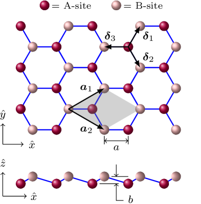
Figure 1: (Color online) Hexagonal lattice of stanene with Sn atoms at A and B sites. The lattice vectors are denoted by $\bm{a}_{1}$ and $\bm{a}_{2}$, and we show the unit cell with a gray rhombus. The interatomic distance projected on the plane is $a$, and along the vertical direction it is $b$, so the interatomic distance is $\sqrt{a^{2}+b^{2}}$.

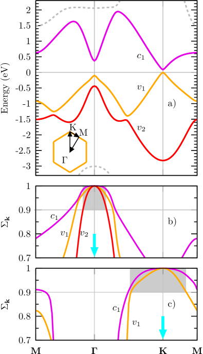
Figure 2: (Color online) a) The ab initio bandstructure of stanene with the bands included in our effective model highlighted. The band gaps at $\mathbf{K}$ and $\mathbf{K}^{\prime}$ have a value of 88 meV. At $\Gamma$, the minimal transition is at 0.472 eV and the second is at 0.808 eV. All bands are doubly (spin) degenerate. The dashed (gray) bands are not described by our model. b) The singular values (the elements of the diagonal matrix $\Sigma_{\mathbf{k}}$, Eq. (4)) with $\mathbf{q}=\mathbf{\Gamma}$ as the reference point. The shaded area indicates the region where the singular values are all greater than $0.9$, and the unitary approximation $\Sigma_{\mathbf{k}}\to\bm{I}$ is acceptable. c) Same as b), but for $\mathbf{q}=\mathbf{K}$ as the reference point.

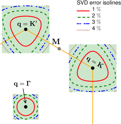
Figure 3: (Color online) Figure of merit of the unitary approximation $\Sigma_{\mathbf{k}}\to\bm{I}$, as defined by Eq. (11), for the three regions of the BZ centered at the reference points $\mathbf{q}=\{\bm{\Gamma},\mathbf{K},\mathbf{K}^{\prime}\}$; each $\mathbf{q}$ is marked with black dots. The yellow lines connecting all contiguous pairs of $\mathbf{K}$ and $\mathbf{K^{\prime}}$ points indicate boundaries of the first Brillouin zone (cf. inset of Fig. 2, a)).

With these structural parameters we proceed to obtain the bandstructure along the typical $\mathbf{M}\bm{\Gamma}\mathbf{K}\mathbf{M}$ path (Fig. 2) in the BZ. All the bands are spin degenerate since stanene has both time-reversal and inversion symmetries. As shown in Fig. 2, the bandstructure of stanene has gaped Dirac cones at the $\mathbf{K}$ and $\mathbf{K}^{\prime}$ points with a gap of $0.088\ e$V. At $\bm{\Gamma}$, the first transition occurs at $0.472\ e$V  and the next one at $0.808\ e$V. At $\mathbf{M}$ the first transition is at $1.55\ e$V; hence we ignore that region of the BZ in our model, as we are focusing on energies up to $1.1\ e$V in this paper. Our effective model contains only states with lattice momentum around the $\mathbf{K}$, $\mathbf{K}^{\prime}$, and $\bm{\Gamma}$ points; it includes 6 bands around the $\bm{\Gamma}$ point and only 4 bands around $\mathbf{K}$ and $\mathbf{K}^{\prime}$ points.

III.1 Accuracy of the approximation for the states

Once the ab initio wavefunctions are computed, we proceed to obtain the overlap matrix (Eq. (3)) between the periodic functions at the reference point $\mathbf{q}$ and the other points in its neighborhood in the BZ; this is done for each of the regions of interest in the BZ, namely the regions around the reference points $\mathbf{K}$, $\mathbf{K}^{\prime}$, and $\bm{\Gamma}$. The overlap matrices of the ab initio wavefunctions can be approximated by unitary matrices based on singular value decompositions according to Eq. (5). In order to determine the region of the BZ where this approximation is accurate, in Fig. 2 we plot the elements of the diagonal matrix $\Sigma_{\mathbf{k}}$ (the singular values) for the reference points $\mathbf{K}$ and $\bm{\Gamma}$; the results for the $\mathbf{K}^{\prime}$ point are similar to those of $\mathbf{K}$. In Fig. 2, we also highlight the regions where each element of $\Sigma_{\mathbf{k}}$ is greater than 0.9, which is taken as our tolerance for the approximation in Eq. (5). Notice that the highlighted regions encompass every point on the BZ where optical transitions with photon energies below $1.1\ e$V are possible.

In order to have a measure of the accuracy of the states that is easier to be visualized, we define a figure of merit

$$\delta_{\Sigma}\left(\mathbf{k}\right)=n^{-1}\,\sqrt{\mathrm{Tr}\left(\Sigma_{\mathbf{k}}-\bm{I}\right)^{2}},$$ (11)

where $n$ is the number of bands included in the model. In Fig. 3 we present the figure of merit $\delta_{\Sigma}\left(\mathbf{k}\right)$ for the three regions of interest in the BZ. We notice that the error indicated by $\delta_{\Sigma}\left(\mathbf{k}\right)$ is lower than 5% for large neighborhoods around the reference points.

III.2 Hamiltonian matrices

Having established the regions where the approximation of the states is valid, we now turn to the approximation of the Hamiltonian matrix. We expand the matrix elements of the Hamiltonian $\bar{H}_{{\bf k}}$ directly as in Eq. (10), and report the results below. Since we use a basis independent of the lattice momentum for the neighborhood of the BZ around each reference point, the Lax connection is null for each of these neighborhoods, $\bar{\bm{\xi}}_{ab\mathbf{k}}=0$.

III.2.1 $\mathbf{K}$ and $\mathbf{K}^{\prime}$ points

The valleys around the $\mathbf{K}$ and $\mathbf{K}^{\prime}$ points are similar in our model, so we present the matrices associated with each of them together, and use the valley parameter $\tau=1$ to refer to $\mathbf{K}$ and $\tau=-1$ to refer to ${\bf K}^{\prime}$. At the $\mathbf{K}$ and $\mathbf{K}^{\prime}$ points, the wavefunctions have a predominant character of $p_{z}$ orbitals located at an atom in the unit cell. We use $s_{i}$ and $\sigma_{i}$ to respectively denote the Pauli matrices in the spin and sublattice sectors; here $i=\left\{0,x,y,z\right\}$, as we adopt the convention of denoting the identity as the zeroth Pauli matrix. In this notation, the Hamiltonian is written in terms of the matrices $s_{i}\otimes\sigma_{j}$.

Up to linear order in the lattice momentum $\bm{\kappa}=\mathbf{k}-\mathbf{q}$, where $\mathbf{q}=\left\{\mathbf{K},\mathbf{K}^{\prime}\right\}$, we find

$$\bar{H}_{\tau\bm{\kappa}}^{\left(1\right)}= \Delta_{K}\left(-\tau s_{z}\otimes\sigma_{z}+s_{0}\otimes\sigma_{0}\right)+\zeta_{K}^{\left(1\right)}as_{0}\otimes\left(\kappa_{x}\sigma_{x}+\tau\kappa_{y}\sigma_{y}\right)$$

$$-\lambda_{K}^{\left(1\right)}a\left(\kappa_{y}s_{x}-\kappa_{x}s_{y}\right)\otimes\sigma_{z},$$ (12)

where in the first term we add an energy shift $\Delta_{K}$ such that the top of the valence band is at zero energy. The quadratic terms in $\bm{\kappa}$ are

$$\bar{H}_{\tau\bm{\kappa}}^{\left(2\right)}= -\zeta_{K}^{\left(2\right)}a^{2}s_{0}\otimes\left[\tau\kappa_{x}\kappa_{y}\sigma_{x}+\frac{1}{2}\left(\kappa_{x}^{2}-\kappa_{y}^{2}\right)\sigma_{y}\right]$$

$$-v_{K}^{\left(2\right)}a^{2}\left|\kappa\right|^{2}s_{0}\otimes\sigma_{0}+\vartheta_{K}^{\left(2\right)}a^{2}\tau\left|\kappa\right|^{2}s_{z}\otimes\sigma_{z}$$ (13)

$$+\eta_{K}^{\left(2\right)}a^{2}\tau\left[\left(\kappa_{x}^{2}-\kappa_{y}^{2}\right)s_{x}-2\kappa_{x}\kappa_{y}s_{y}\right]\otimes\sigma_{z},$$

where the values of the parameters are shown in Table 1. Neglecting the relatively small parameters $\lambda_{K}^{\left(1\right)}$ and $\eta_{K}^{(2)}$ leads to a separation of the spin subsectors, since without them $\bar{H}_{\tau{\bf k}}^{\left(1\right)}$ and $\bar{H}_{\tau{\bf k}}^{\left(2\right)}$ do not have terms with $s_{x}$ and $s_{y}$, the only matrices with cross-spin elements. The spin separation is expected for lattices without buckling, and it indicates that the lattice buckling can be neglected in calculations involving $\mathbf{k}$ close to the expansion point $\mathbf{q}$.

The parameters $v_{K}^{\left(2\right)}$ and $\vartheta_{K}^{\left(2\right)}$ can also be neglected, and the three parameters $\Delta_{K}$, $\zeta_{K}^{\left(1\right)}$ and $\zeta_{K}^{\left(2\right)}$ are the only ones needed for our model to give band energies that match those from DFT within a tolerance of room temperature energy. We nevertheless report the negligible parameters $\lambda_{K}^{\left(1\right)}$, $\eta_{K}^{(2)}$, $v_{K}^{\left(2\right)}$ and $\vartheta_{K}^{\left(2\right)}$, because their physical significance can be identified with the help of a $p_{z}$-orbital tight-binding model, as we discuss in the Appendix. Finally, we provide an analytical expression for the band energies around the $\mathbf{K}$ and $\mathbf{K}^{\prime}$ points obtained from our effective model. Neglecting the small parameters mentioned in the previous paragraph, we have

$$E_{\tau\bm{\kappa}}^{\pm} =\Delta_{K}\pm\sqrt{\Delta_{K}^{2}+\mathcal{X}_{\bm{\kappa}}^{2}+\mathcal{Y}_{\bm{\kappa}}^{2}},$$ (14a)

$$\mathcal{X}_{\bm{\kappa}} =a\kappa_{x}\left(\zeta_{K}^{\left(1\right)}-\tau\zeta_{K}^{\left(2\right)}a\kappa_{y}\right),$$ (14b)

$$\mathcal{Y}_{\bm{\kappa}} =\zeta_{K}^{\left(1\right)}a\kappa_{y}-\frac{1}{2}\tau\zeta_{K}^{\left(2\right)}a^{2}\left(\kappa_{x}^{2}-\kappa_{y}^{2}\right),$$ (14c)

where the positive and negative signs of the square root correspond to the conduction and valence bands respectively.

All values in eV
$\Delta_{K}=0.044$	$\zeta_{K}^{\left(1\right)}=0.67$	$\zeta_{K}^{\left(2\right)}=0.33$
	$\lambda_{K}^{\left(1\right)}=0.03$	$v_{K}^{\left(2\right)}=0.03$
		$\vartheta_{K}^{\left(2\right)}=0.03$
		$\eta_{K}^{\left(2\right)}=0.02$

Table 1: Parameter values of the models for the $\mathbf{K}$ and $\mathbf{K^{\prime}}$ valleys in the BZ, see Eqs. (III.2.1) and (III.2.1). The parameters $\lambda_{K}^{\left(1\right)}$, $\eta_{K}^{(2)}$, $v_{K}^{\left(2\right)}$ and $\vartheta_{K}^{\left(2\right)}$ can be neglected without significant changes in the band energies. Neglecting the parameters $\lambda_{K}^{\left(1\right)}$ and $\eta_{K}^{(2)}$ alone already leads to a separation of the spin subsectors.

III.2.2 $\bm{\Gamma}$ point

At the $\mathbf{\Gamma}$ point, the wavefunctions cannot be easily associated with a sublattice, but they can still be identified according to spin, so we continue using $s_{i}$ to denote the Pauli matrices acting on the spin sector of the Hilbert space. Up to linear order in the lattice momentum, here $\bm{\kappa}=\mathbf{k}-\mathbf{q}=\mathbf{k}$ since $\mathbf{q}=\bm{\Gamma}$, we find

$$\begin{array}[]{rl}\bar{H}_{\Gamma\bm{\kappa}}^{\left(1\right)}=&s_{0}\otimes\begin{bmatrix}E_{\Gamma}^{\left(c\right)}&0&0\\ 0&E_{\Gamma}^{\left(v1\right)}&0\\ 0&0&E_{\Gamma}^{\left(v2\right)}\end{bmatrix}+a\kappa_{x}s_{0}\otimes\begin{bmatrix}0&\zeta_{\Gamma 1}^{\left(1\right)}&\zeta_{\Gamma 2}^{\left(1\right)}\\ \zeta_{\Gamma 1}^{\left(1\right)}&0&0\\ \zeta_{\Gamma 2}^{\left(1\right)}&0&0\end{bmatrix}\\ &+a\kappa_{y}s_{z}\otimes\begin{bmatrix}0&-i\zeta_{\Gamma 1}^{\left(1\right)}&i\zeta_{\Gamma 2}^{\left(1\right)}\\ i\zeta_{\Gamma 1}^{\left(1\right)}&0&0\\ -i\zeta_{\Gamma 2}^{\left(1\right)}&0&0\end{bmatrix},\end{array}$$ (15)

while the quadratic terms in $\bm{\kappa}$ are

$$\begin{array}[]{rl}\bar{H}_{\Gamma\bm{\kappa}}^{\left(2\right)}=&\frac{1}{2}a^{2}\left|\kappa\right|^{2}s_{0}\otimes\begin{bmatrix}v_{\Gamma c}^{\left(2\right)}&0&0\\ 0&-v_{\Gamma 1}^{\left(2\right)}&0\\ 0&0&-v_{\Gamma 2}^{\left(2\right)}\end{bmatrix}\\ &+\frac{1}{2}a^{2}\left(\kappa_{x}^{2}-\kappa_{y}^{2}\right)s_{0}\otimes\begin{bmatrix}0&0&0\\ 0&0&\zeta_{\Gamma v}^{\left(2\right)}\\ 0&\zeta_{\Gamma v}^{\left(2\right)}&0\end{bmatrix}\\ &+a^{2}\kappa_{x}\kappa_{y}s_{z}\otimes\begin{bmatrix}0&0&0\\ 0&0&i\zeta_{\Gamma v}^{\left(2\right)}\\ 0&-i\zeta_{\Gamma v}^{\left(2\right)}&0\end{bmatrix}.\end{array}$$ (16)

The values of the parameters are presented in Table 2. Here we have omitted negligible parameters. The parameters reported constitute the minimum set necessary to describe the energies with an accuracy equivalent to room temperature when compared to the bands from DFT. Notice that the model for the valley at the $\mathbf{\Gamma}$ point can also be separated in two spin sectors.

All values in $e$V
$E_{\Gamma}^{c}=0.37$	$\zeta_{\Gamma 1}^{\left(1\right)}=1.23$	$v_{\Gamma c}^{\left(2\right)}=0.34$
$E_{\Gamma}^{v1}=-0.10$	$\zeta_{\Gamma 2}^{\left(1\right)}=1.16$	$v_{\Gamma 1}^{\left(2\right)}=0.45$
$E_{\Gamma}^{v2}=-0.44$		$v_{\Gamma 2}^{\left(2\right)}=0.34$
		$\zeta_{\Gamma v}^{\left(2\right)}=0.35$

Table 2: Parameter values of the model for the $\mathbf{\Gamma}$ valley, see Eqs. (15) and (16). Negligible parameters are omitted.

III.3 Accuracy of the energies

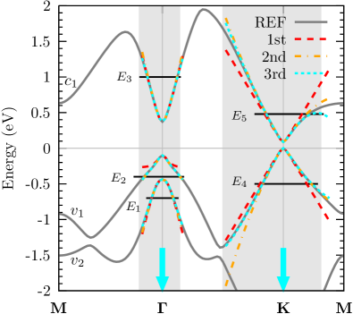
Figure 4: (Color online) Comparison of the band energies obtained from the Taylor expansions of the Hamiltonian matrices (dashed lines) in Sec. III.2 with those from the ab initio calculation (continuous gray line). The band energies from the effective model are plotted only in the shaded regions, where approximation for the states is accurate as discussed in Sec. III.1.

The accuracy of the Taylor expansion of the Hamiltonian matrices in the previous subsection can be determined by comparing the band energies obtained from our model with those from the ab initio calculation. In Fig. 4 we present the band energies obtained from models including first-, second-, and third-order expansions of the Hamiltonian on the lattice momentum difference $\bm{\kappa}$; third-order expansions are not discussed further in this work. We also show the ab initio bands for comparison, and focus on the regions where the approximation for the states is accurate as discussed in Sec. III.1. From Fig. 4, we see that keeping the cubic terms in the Hamiltonian expansion is unnecessary to reproduce the ab initio band energies around the $\bm{\Gamma}$ point, while for the region around the $\mathbf{K}$ point (and equivalently the $\mathbf{K}^{\prime}$ point) it is actually detrimental to go beyond the second-order expansion.

A plot of band energies along a simple path through a region of the BZ is not enough to establish the accuracy of the bands from our model in that entire region. Analyzing the band warping is a way to ensure that the good agreement displayed in Fig. 4 is not coincidental to the directions associated with that plot. In Fig. 5 we show isoenergy lines for each relevant band obtained from our model and those from the ab initio computation. The latter are shown as pairs of lines that enclose an energy range equivalent to room temperature, which is taken as our tolerance for energy accuracy. We compare the band warping corresponding to expansions of the Hamiltonian that are quadratic and cubic on the lattice momentum difference $\bm{\kappa}$; on Fig. 5 we show that the cubic expansion does not improve upon the quadratic one. Thus we confirm that the quadratic expansion provides the best model for the bandstructure of stanene for excitation energies up to $1.1\ e$V.

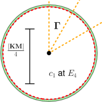
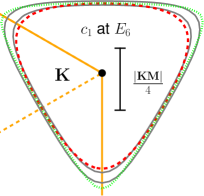
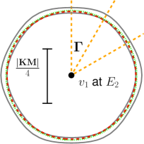
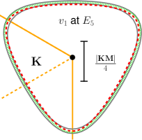
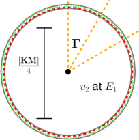
Figure 5: (Color online) Trigonal warping of the relevant bands around the reference points in the BZ in our model. Red-dashed and green-dotted lines indicate respectively second and third order expansions of the Hamiltonian matrices. The thin gray lines are ab initio energy isolines that enclose a range of energy equivalent to room temperature. To give a sense of proportion we include a line segment of length one fourth of the distance $\overline{\mathbf{KM}}$. The isolevels $E_{i}$ and band labels $v_{i}$ and $c_{1}$ are as indicated in Fig. 4.

IV Optical properties

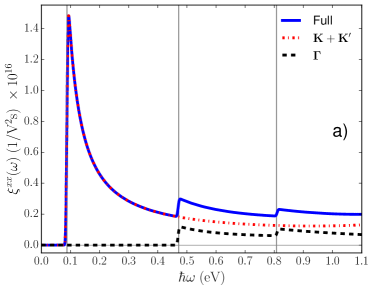
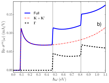
Figure 6: (Color online) Linear optical absorption properties computed with the effective model of Sec. III.1. a) One-photon absorption coefficient $\xi^{xx}\left(\omega\right)$ and b) real part of the optical conductivity $\sigma^{xx}\left(\omega\right)$ of stanene. The contributions from the regions around the $\mathbf{K}$ and $\mathbf{K}^{\prime}$ points (dot-dashed red line) and the $\bm{\Gamma}$ point (dashed black line) in the BZ are shown separately, along with that from the full BZ (solid blue line); we stress that the “full” signal indeed contains contributions from all crystal momenta $\mathbf{k}$ around $\mathbf{K}(\mathbf{K^{\prime}})$ and $\mathbf{\Gamma}$ for which one-photon transitions less than 1.1 eV are possible; consequently, it is equivalent to a full BZ calculation, within the limits of validity of our model.

The optical properties of a crystalline system depend only on the Hamiltonian matrix and the Lax connection Muniz and Sipe (2017). Since the Lax connection is null in the basis of our model $\bar{\bm{\xi}}_{ab\mathbf{k}}=0$, the velocity matrix elements are simply given by $\bm{v}\left(\mathbf{k}\right)=\hbar^{-1}\bm{\nabla}_{\mathbf{k}}\bar{H}\left(\mathbf{k}\right)$. We consider the optical injection rates of carrier and spin densities, given by

$$\frac{d}{dt}n =\xi^{ab}\left(\omega\right)E^{a}\left(\omega\right)\,E^{b}\left(-\omega\right),$$ (17)

$$\frac{d}{dt}S^{z} =\zeta^{zab}\left(\omega\right)E^{a}\left(\omega\right)\,E^{b}\left(-\omega\right),$$ (18)

where we use the convention of summing repeated indices, ${\bf E}\left(t\right)={\bf E}\left(\omega\right)e^{-i\omega t}+c.c.$ is an incident optical field, and the tensors $\xi^{ab}\left(\omega\right)$ and $\zeta^{zab}\left(\omega\right)$ are the carrier and spin density injection coefficients

$$\xi^{ab}\left(\omega\right) =\dfrac{2\pi e^{2}}{\hbar^{2}\omega^{2}}\underset{cv}{\sum}\int\dfrac{d^{2}k}{\left(2\pi\right)^{2}}v_{cv{\bf k}}^{a}v_{vc{\bf k}}^{b}\delta\left(\omega-\omega_{cv{\bf k}}\right),$$ (19)

$$\zeta^{zab}\left(\omega\right) =\dfrac{2\pi e^{2}}{\hbar^{2}\omega^{2}}\underset{cv}{\sum}\int\dfrac{d^{2}k}{\left(2\pi\right)^{2}}\left(S_{cc}^{z}-S_{vv}^{z}\right)v_{cv{\bf k}}^{a}v_{vc{\bf k}}^{b}\delta\left(\omega-\omega_{cv{\bf k}}\right),$$ (20)

where $v$ and $c$ are respectively valence and conduction band indices, $e=-|e|$ is the electron charge, $v_{cv{\bf k}}^{a}$ are the velocity matrix elements, $S_{cc}^{z}=\pm\hbar/2$ and $S_{vv}^{z}=\mp\hbar/2$ are the spin-$\hat{{\bf z}}$ matrix elements of respectively the conduction and valence bands, and $\hbar\omega_{cv\bm{k}}=\hbar\omega_{c\bm{k}}-\hbar\omega_{v\bm{k}}$ are band energy differences. In numerical calculations, we approximate the Dirac delta function in the above equations by a Lorentzian function with a broadening width of $6$ m$e$V.

In Fig. 6, we present plots of the linear optical absorption coefficient $\xi^{xx}\left(\omega\right)$ and the real part of the optical conductivity ${\rm Re}\sigma^{xx}\left(\omega\right)$, which are related to each other by $\xi^{xx}\left(\omega\right)=2\mathrm{Re\,}\sigma^{xx}\left(\omega\right)/\left(\hbar\omega\right)$. As the frequency increases, the absorption begins at the band gap energy $0.088\ e$V due to electronic transitions at the $\mathbf{K}$ and $\mathbf{K}^{\prime}$ valleys in the BZ. The contribution from $\mathbf{\Gamma}$ has an absorption onset at $0.472\ e$V, and a second absorption onset at $0.808\ e$V, when electronic transitions from the second valence band are allowed.

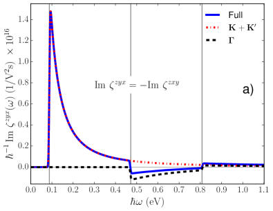
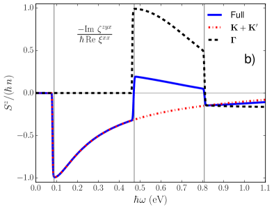
Figure 7: (Color online) Spin density injection computed with the effective model of Sec. III.1. a) Spin density injection coefficient $\zeta^{zyx}\left(\omega\right)$ and b) Spin polarization of injected carriers with circularly polarized light $-{\rm Im}\,\zeta^{zyx}\left(\omega\right)/\left[\hbar\xi^{xx}\left(\omega\right)\right]$ for stanene, with $\mathfrak{h}=1$. The contributions from the regions around the $\mathbf{K}$ and $\mathbf{K}^{\prime}$ points (dot-dashed red line) and the $\bm{\Gamma}$ point (dashed black line) in the BZ are shown separately, along with that from the full BZ (solid blue line), in the sense described in the caption of Fig. 6.

For photon energies close to the band gap, stanene has the interesting property that circularly polarized light excites mostly electrons with the spin that matches its helicity. Similar characteristics have been identified and studied in other monolayers, such as siliceneEzawa (2012a). This feature can be seen from our linear model for the $\mathbf{K}$ and $\mathbf{K}^{\prime}$ points in Eq. III.2.1, which can be separated in spin sectors, and the expressions of $\xi\left(\omega\right)$ and $\zeta\left(\omega\right)$ for a Dirac cone Muniz and Sipe (2014, 2015). For circular polarizations, the light field propagating along the $\hat{{\bf z}}$ direction can be written as ${\bf E}\left(\omega\right)=E_{\omega}\hat{{\bf p}}_{\mathfrak{h}}$, where $\mathfrak{h}=\pm 1$ is the helicity, and $\hat{{\bf p}}_{\mathfrak{h}}=\left(\hat{{\bf x}}+i\mathfrak{h}\hat{{\bf y}}\right)/\sqrt{2}$. Then the expression for each spin $s=\pm 1$ is

$$\xi_{\tau s}^{\mathfrak{h}}\left(\omega\right)= \frac{\Theta\left(\omega-2\Delta_{K}\right)e^{2}}{8\hbar^{2}\omega}\left(1+\mathfrak{h}s\frac{2\Delta_{K}}{\omega}\right)^{2},$$ (21)

which is independent of valley, and where $\Theta\left(x\right)$ is the step function, valued as zero or unity if $x<0$ or $x>0$, respectively. From Eq. (21) we see that the spin polarization is maximal for photon energies corresponding to the gap, and it decreases for larger photon energies. The injection coefficient of an arbitrary quantity for circularly polarized light, $\eta^{\mathfrak{h}}\left(\omega\right)$, is given in terms of its Cartesian components as

$$\eta^{\mathfrak{h}}\left(\omega\right) =\frac{1}{2}\left[\eta^{xx}\left(\omega\right)+\eta^{yy}\left(\omega\right)\right]+i\mathfrak{h}\frac{1}{2}\left[\eta^{yx}\left(\omega\right)-\eta^{xy}\left(\omega\right)\right]$$

$$=\eta^{xx}\left(\omega\right)+i\,\mathfrak{h}\,\eta^{yx}\left(\omega\right),$$ (22)

where the relations $\eta^{xx}\left(\omega\right)=\eta^{yy}\left(\omega\right)$ and $\eta^{yx}\left(\omega\right)=-\eta^{xy}\left(\omega\right)$ due to the symmetries of a buckled honeycomb lattice were used. For carrier and spin densities in stanene, we also have $\xi^{xx}\left(\omega\right)={\rm Re}\,\xi^{xx}\left(\omega\right)$ and $\xi^{yx}\left(\omega\right)=0$, as well as $\zeta^{zxx}\left(\omega\right)=0$ and $\zeta^{zyx}\left(\omega\right)=i\,{\rm Im}\,\zeta^{zyx}\left(\omega\right)$. So the coefficients for circular polarizations are simply $\xi^{\mathfrak{h}}\left(\omega\right)={\rm Re}\,\xi^{xx}\left(\omega\right)$ and $\zeta^{\mathfrak{h}}\left(\omega\right)=-\mathfrak{h}\,{\rm Im}\,\zeta^{zyx}\left(\omega\right)$. We present plots of the spin density injection coefficient $\zeta^{zxy}\left(\omega\right)$ computed with our effective model in Fig. 7 a), which shows the same frequency regimes discussed for $\xi^{xx}\left(\omega\right)$. In Fig. 7 b) we show the spin polarization of injected carriers for circularly polarized light. Even for excitations at the $\mathbf{\Gamma}$ valley there is still a helicity-spin coupling, although the net spin polarization is partially canceled by the excitations at the $\mathbf{K}$ and $\mathbf{K}^{\prime}$ valleys.

We note that helicity-spin coupling is due to the sign of the mass term $\Delta_{K}$ in each Dirac cone Ryu et al. (2009); Santos et al. (2010); Chamon et al. (2012), which also explains why stanene shows the spin Hall effect. We also point out that the helicity-spin coupling in stanene is analogous to the helicity-valley coupling in TMDs Xiao et al. (2012).

V Conclusions

We have presented an effective model that accurately describes the electronic and optical properties of stanene for low photon energies. We started from an ab initio calculation of the bandstructure of stanene, which allowed us to identify the parameters in the model. Our model includes a minimum set of energy states: 6 bands around the $\mathbf{\Gamma}$ point in the BZ, and 4 bands around the $\mathbf{K}$ and $\mathbf{K}^{\prime}$ points. We provided measures for the accuracy of the approximations for states and for energies, so we can identify the range of validity of the model.

We found that a quadratic model with respect to the lattice momentum is the best suited for calculations based on the bandstructure. Even the band warping from DFT calculations is better reproduced by the quadratic rather than a cubic model. We also found that the lattice buckling can be neglected. This is confirmed by verifying that a separation of the states according to spin-$\hat{{\bf z}}$ subsectors is a good approximation for the band energies. In the Appendix, we discuss the physical significance of some parameters in our model by comparing it to a $p_{z}$-orbital tight-binding model expanded around the ${\bf K}$ and ${\bf K}^{\prime}$ regions of the BZ. Finally, we illustrated the applicability of the model by computing linear optical absorption rates of stanene. We highlighted the coupling of circularly polarized light with the electronic spin, which underscores the potential of stanene for optical-spintronic applications.

The model proposed here can accurately describe optical properties of stanene up to photon energies of $1.1\ e$V, which is suitable for a wide range of optical experiments. Compared with a usual $\mathbf{k}\cdot\mathbf{p}$ method, our model requires fewer parameters to describe the bandstructure; we also provide a figure of merit to determine the portion of the Brillouin Zone where the approximation is sensible. We expect that this simple model will be useful in understanding and suggesting experiments on this promising material, and that the procedure described here will be used to extract effective models from ab initio calculations for other 2D materials.

Appendix A Tight binding model

Tight-binding models (TBM) have successfully been used to describe electronic states in the full Brillouin zone (BZ) in different monolayer materials, such as silicene, germanene and staneneLiu et al. (2011); Ezawa (2012b); the description of the full BZ usually requires the inclusion of basis sets with $s$, $p_{x}$, $p_{y}$ and $p_{z}$ orbitals. In this Appendix we discuss a TBM that includes only $p_{z}$ orbitals on a buckled honeycomb lattice, which is enough to describe the states around the $\mathbf{K}$ and $\mathbf{K}^{\prime}$ points in the BZ, and in that region it agrees with the models of Liu Liu et al. (2011) and Ezawa Ezawa (2012b). This TBM is unable to describe the states at the $\bm{\Gamma}$ point because their orbital character are not purely $p_{z}$. For instance, from a DFT calculation, we find that at the $\bm{\Gamma}$ point the orbital character of the first conduction band is 73% $s$, 24% $p_{z}$ and 3% $d$, while that of the top valence band is 96% a mix of $p_{x}$ and $p_{y}$, and about 4% $d$ character. We assume that the orbitals are well localized and we apply a change of basis to the $B$ sublattice $u_{B\mathbf{k}}\left(\mathbf{r}\right)\to e^{-i\mathbf{k}\cdot\bm{\delta}_{3}}u_{B\mathbf{k}}\left(\mathbf{r}\right)$ in order to have a basis with vanishing Lax connection.

This basis is not in Bloch’s form, and it allows us to write all the hopping parameters in terms of the nearest neighbor vectors $\bm{\delta}_{n}$ instead of the lattice vectors $\bm{a}_{n}$. Using the notation employed in the main text, the Hamiltonian is written in terms of the matrices $s_{i}\otimes\sigma_{j}$. With these conventions and employing a usual tight-binding frameworkCastro Neto et al. (2009), the nearest-neighbour (NN) hopping term in the Hamiltonian is

$$\begin{array}[]{rl}{\cal H}_{\mathbf{k}}^{\mathrm{NN}}=&-t\underset{n=1}{\overset{3}{\sum}}s_{0}\otimes\left[\begin{array}[]{cc}0&e^{-i\mathbf{k}\cdot\bm{\delta}_{n}}\\ e^{i\mathbf{k}\cdot\bm{\delta}_{n}}&0\end{array}\right]\\ =&-t\underset{n=1}{\overset{3}{\sum}}s_{0}\otimes\left[\cos\left(\mathbf{k}\cdot\bm{\delta}_{n}\right)\sigma_{x}+\sin\left(\mathbf{k}\cdot\bm{\delta}_{n}\right)\sigma_{y}\right],\end{array}$$ (23)

and the next-nearest-neighbor (NNN) term is

$$\begin{array}[]{rl}{\cal H}_{\mathbf{k}}^{\mathrm{NNN}}=&-t^{\prime}\underset{n,m\neq n}{\sum}\left[e^{i\mathbf{k}\cdot\left(\bm{\delta}_{m}-\bm{\delta}_{n}\right)}+e^{-i\mathbf{k}\cdot\left(\bm{\delta}_{m}-\bm{\delta}_{n}\right)}\right]s_{0}\otimes\sigma_{0}\\ =&-2t^{\prime}\underset{n,m\neq n}{\sum}\cos\left(\mathbf{k}\cdot\left(\bm{\delta}_{m}-\bm{\delta}_{n}\right)\right)s_{0}\otimes\sigma_{0},\end{array}$$ (24)

without the spin-orbit coupling. The spin-orbit coupling changes the next-nearest-neighbor hopping matrices according to

$$t^{\prime}s_{0}\otimes\sigma_{0}\to t^{\prime}s_{0}\otimes\sigma_{0}+i\lambda_{SO}\left(\hat{\bm{\delta}}_{m}\times\hat{\bm{\delta}}_{n}\right)\cdot{\bf s}\otimes\sigma_{z},$$ (25)

where $\lambda_{SO}$ is the spin-orbit coupling parameter. The last term in the above equation can be further separated in two parts by decomposing the $\hat{\bm{\delta}}_{m}\times\hat{\bm{\delta}}_{n}$ vector as

$$\lambda_{SO}\hat{\bm{\delta}}_{m}\times\hat{\bm{\delta}}_{n}=\lambda_{z}\hat{{\bf z}}+\lambda_{b}\hat{{\bf z}}\times\left(\bm{\delta}_{m}-\bm{\delta}_{n}\right),$$ (26)

where

$$\lambda_{z} =\dfrac{a}{\sqrt{a^{2}+4b^{2}}}\lambda_{SO},\negthickspace \lambda_{b} =\dfrac{2b}{\sqrt{a^{2}+4b^{2}}}\lambda_{SO},$$ (27)

according to the lattice buckling; the lattice parameters $a$ and $b$ are depicted in Fig. 1.

In order to compare the tight-binding model with the one described in Sec. A, we now perform an expansion in powers of $\bm{\kappa}$ around the $\mathbf{K}$ and $\mathbf{K}^{\prime}$ points in the BZ, to which we respectively associate $\tau=+1$ and $\tau=-1$. Here we do not consider the effect of a substrate, hence $\mu=0$ and $\lambda_{R}=0$, so we are describing suspended stanene. Applying a further change of basis to the $B$ sublattice, $u_{B\mathbf{k}}\left(\mathbf{r}\right)\to ie^{i{\bf K}\cdot\bm{\delta}_{3}}u_{B\mathbf{k}}\left(\mathbf{r}\right)$, the linear term is

$$\begin{array}[]{rl}{\cal H}_{\tau\bm{\kappa}}^{\left(1\right)}=&-\tau\frac{9}{2}\lambda_{z}a^{2}s_{z}\otimes\sigma_{z}+\frac{3}{2}tas_{0}\otimes\left(\kappa_{x}\sigma_{x}+\tau\kappa_{y}\sigma_{y}\right)\\ &+3t^{\prime}s_{0}\otimes\sigma_{0}-\frac{9}{2}\lambda_{b}a^{3}\left(\kappa_{y}s_{x}-\kappa_{x}s_{y}\right)\otimes\sigma_{z},\end{array}$$ (28)

where the term $3t^{\prime}s_{0}\otimes\sigma_{0}$ is simply an energy shift and can be removed. The quadratic term is

$$\begin{array}[]{rl}{\cal H}_{\tau\bm{\kappa}}^{\left(2\right)}=&-\frac{3}{4}ta^{2}s_{0}\otimes\left[\tau\kappa_{x}\kappa_{y}\sigma_{x}+\frac{1}{2}\left(\kappa_{x}^{2}-\kappa_{y}^{2}\right)\sigma_{y}\right]\\ &-\frac{9}{4}t^{\prime}a^{2}\kappa^{2}s_{0}\otimes\sigma_{0}+\left(\frac{3}{2}\right)^{3}\lambda_{z}a^{4}\tau\kappa^{2}s_{z}\otimes\sigma_{z}\\ &+\left(\frac{3}{2}\right)^{3}\lambda_{b}a^{4}\tau\left[\left(\kappa_{x}^{2}-\kappa_{y}^{2}\right)s_{x}-2\kappa_{x}\kappa_{y}s_{y}\right]\otimes\sigma_{z}.\end{array}$$ (29)

Now we compare this tight-binding model described by Eqs. (28)-(29) to our effective model around the $\mathbf{K}$ and $\mathbf{K}^{\prime}$ points in the BZ described by Eqs. (III.2.1)-(III.2.1). The relations between the respective first order parameters are

$$\Delta_{K}= \tfrac{9}{2}\lambda_{z}a^{2}, \zeta_{K}^{\left(1\right)}= \tfrac{3}{2}t, \lambda_{K}^{\left(1\right)}= \tfrac{9}{2}\lambda_{b}a^{2},$$ (30)

and for the second order ones, we have

$$\zeta_{K}^{\left(2\right)}= \tfrac{3}{4}t, v_{K}^{\left(2\right)}= \tfrac{9}{4}t^{\prime}, \vartheta_{K}^{\left(2\right)}= \left(\tfrac{3}{2}\right)^{3}\lambda_{z}a^{2}, \eta_{K}^{\left(2\right)}= \left(\tfrac{3}{2}\right)^{3}\lambda_{b}a^{2},$$ (31)

Since $\lambda_{b}=2b\lambda_{z}/a$, we can take $t$, $t^{\prime}$ and $\lambda_{z}$ to be the only independent parameters of the tight-binding model; numerical values for them can be obtained from Table I. Consequently,

$$\lambda_{K}^{\left(1\right)}= \frac{2b}{a}\Delta_{K}, \zeta_{K}^{\left(2\right)}= \frac{1}{2}\zeta_{K}^{\left(1\right)}, \vartheta_{K}^{\left(2\right)}= \frac{3}{4}\Delta_{K}, \eta_{K}^{\left(2\right)}= \frac{3b}{2a}\Delta_{K}.$$ (32)

This tells us that $\Delta_{K}$, $\zeta_{K}^{\left(1\right)}$ and $v_{K}^{\left(2\right)}$ can be taken as the only independent parameters in Table 1, just as the 3 independent parameters for the tight-binding. The parameters $t^{\prime}$ and $v_{K}^{\left(2\right)}$ can be neglected, though, so the relevant parameters are only two: $t$ and $\lambda_{z}$ for tight-binding, and $\Delta_{K}$ and $\zeta_{K}^{\left(1\right)}$ in our effective model. The relations above are satisfied by the parameters shown in Table 1.

References

- Miro et al. (2014) P. Miro, M. Audiffred, and T. Heine, Chem. Soc. Rev. 43, 6537 (2014).
- Gupta et al. (2015) A. Gupta, T. Sakthivel, and S. Seal, Progress in Materials Science 73, 44 (2015).
- Ezawa (2015) M. Ezawa, Journal of the Physical Society of Japan 84, 121003 (2015).
- Ezawa and Lay (2015) M. Ezawa and G. L. Lay, New Journal of Physics 17, 090201 (2015).
- Zhao et al. (2016) J. Zhao, H. Liu, Z. Yu, R. Quhe, S. Zhou, Y. Wang, C. C. Liu, H. Zhong, N. Han, J. Lu, et al., Progress in Materials Science 83, 24 (2016).
- Sahoo et al. (2016) T. Sahoo, S. K. Nayak, P. Chelliah, M. K. Rath, and B. Parida, Materials Research Bulletin 75, 134 (2016).
- Wang et al. (2012) Q. H. Wang, K. Kalantar-Zadeh, A. Kis, J. N. Coleman, and M. S. Strano, Nat Nano 7, 699 (2012).
- Xu et al. (2014) X. Xu, W. Yao, D. Xiao, and T. F. Heinz, Nat Phys 10, 343 (2014).
- Houssa et al. (2014) M. Houssa, B. van den Broek, E. Scalise, B. Ealet, G. Pourtois, D. Chiappe, E. Cinquanta, C. Grazianetti, M. Fanciulli, A. Molle, et al., Applied Surface Science 291, 98 (2014).
- Bianco et al. (2013) E. Bianco, S. Butler, S. Jiang, O. D. Restrepo, W. Windl, and J. E. Goldberger, ACS Nano 7, 4414 (2013), pMID: 23506286.
- Acun et al. (2015) A. Acun, L. Zhang, P. Bampoulis, M. Farmanbar, A. van Houselt, A. N. Rudenko, M. Lingenfelder, G. Brocks, B. Poelsema, M. I. Katsnelson, et al., Journal of Physics: Condensed Matter 27, 443002 (2015).
- Özçelik et al. (2015) V. O. Özçelik, O. Üzengi Aktürk, E. Durgun, and S. Ciraci, Phys. Rev. B 92 (2015).
- Pereira and Katsnelson (2015) J. M. Pereira and M. I. Katsnelson, Phys. Rev. B 92 (2015).
- Kamal and Ezawa (2015) C. Kamal and M. Ezawa, Phys. Rev. B 91, 085423 (2015).
- Üzengi Aktürk et al. (2015) O. Üzengi Aktürk, V. O. Özçelik, and S. Ciraci, Phys. Rev. B 91 (2015).
- Pizzi et al. (2016) G. Pizzi, M. Gibertini, E. Dib, N. Marzari, G. Iannaccone, and G. Fiori, Nature Communications 7, 12585 (2016).
- Aktürk et al. (2016) E. Aktürk, O. Üzengi Aktürk, and S. Ciraci, Phys. Rev. B 94 (2016).
- Mannix et al. (2015) A. J. Mannix, X.-F. Zhou, B. Kiraly, J. D. Wood, D. Alducin, B. D. Myers, X. Liu, B. L. Fisher, U. Santiago, J. R. Guest, et al., Science 350, 1513 (2015).
- Fregoso et al. (2016) Fregoso, Morimoto, and Moore (2016), URL https://arxiv.org/abs/1701.00172.
- Xu et al. (2013) Y. Xu, B. Yan, H.-J. Zhang, J. Wang, G. Xu, P. Tang, W. Duan, and S.-C. Zhang, Phys. Rev. Lett. 111, 136804 (2013).
- van den Broek et al. (2014) B. van den Broek, M. Houssa, E. Scalise, G. Pourtois, V. V. Afanas’ev, and A. Stesmans, 2D Materials 1, 021004 (2014).
- Zhu et al. (2015) F.-f. Zhu, W.-j. Chen, Y. Xu, C.-l. Gao, D.-d. Guan, C.-h. Liu, D. Qian, S.-C. Zhang, and J.-f. Jia, Nat Mater 14, 1020 (2015).
- Saxena et al. (2016) S. Saxena, R. P. Chaudhary, and S. Shukla, Scientific Reports 6, 31073 (2016).
- Chaudhary et al. (2016) R. P. Chaudhary, S. Saxena, and S. Shukla, Nanotechnology 27, 495701 (2016).
- Willatzen and Yan Voon (2009) M. Willatzen and L. Yan Voon, The Method (Springer, 2009).
- Marzari and Vanderbilt (1997) N. Marzari and D. Vanderbilt, Phys. Rev. B 56, 12847 (1997).
- Marzari et al. (2012) N. Marzari, A. A. Mostofi, J. R. Yates, I. Souza, and D. Vanderbilt, Rev. Mod. Phys. 84, 1419 (2012).
- Cardona and Pollak (1966) M. Cardona and F. H. Pollak, Phys. Rev. 142, 530 (1966).
- Richard et al. (2004) S. Richard, F. Aniel, and G. Fishman, Phys. Rev. B 70, 235204 (2004).
- Cheng et al. (2013) J. L. Cheng, C. Salazar, and J. E. Sipe, Phys. Rev. B 88, 045438 (2013).
- Gonze et al. (2009) X. Gonze et al., Comput. Phys. Commun. 180, 2582 (2009).
- Gonze et al. (2016) X. Gonze et al., Comput. Phys. Commun. 205, 106 (2016).
- Hamann (2013) D. R. Hamann, Phys. Rev. B 88, 085117 (2013).
- Cahangirov et al. (2009) S. Cahangirov, M. Topsakal, E. Aktürk, H. Şahin, and S. Ciraci, Phys. Rev. Lett. 102, 236804 (2009).
- Muniz and Sipe (2017) R. A. Muniz and J. E. Sipe, arXiv (2017).
- Ezawa (2012a) M. Ezawa, Phys. Rev. B 86, 161407 (2012a).
- Muniz and Sipe (2014) R. A. Muniz and J. E. Sipe, Phys. Rev. B 89, 205113 (2014).
- Muniz and Sipe (2015) R. A. Muniz and J. E. Sipe, Phys. Rev. B 91, 085404 (2015).
- Ryu et al. (2009) S. Ryu, C. Mudry, C.-Y. Hou, and C. Chamon, Phys. Rev. B 80, 205319 (2009).
- Santos et al. (2010) L. Santos, S. Ryu, C. Chamon, and C. Mudry, Phys. Rev. B 82, 165101 (2010).
- Chamon et al. (2012) C. Chamon, C.-Y. Hou, C. Mudry, S. Ryu, and L. Santos, Physica Scripta 2012, 014013 (2012).
- Xiao et al. (2012) D. Xiao, G.-B. Liu, W. Feng, X. Xu, and W. Yao, Phys. Rev. Lett. 108, 196802 (2012).
- Liu et al. (2011) C.-C. Liu, H. Jiang, and Y. Yao, Phys. Rev. B 84, 195430 (2011).
- Ezawa (2012b) M. Ezawa, New J. Phys 14 (2012b).
- Castro Neto et al. (2009) A. H. Castro Neto, F. Guinea, N. M. R. Peres, K. S. Novoselov, and A. K. Geim, Rev. Mod. Phys. 81, 109 (2009).
- Lax (2012) M. Lax, Symmetry Principles in Solid State and Molecular Physics (Dover Publications, 2012), reprint of the John Wiley & Sons, 1974 edition.