Edinburgh 2017/11, IPPP/17/33, DCPT/17/66, MCnet-17-9 Higgs Boson Plus Dijets: Higher Order Corrections

Abstract

The gluon fusion component of Higgs-boson production in association with dijets is of particular interest because it both (a) allows for a study of the $CP$-structure of the Higgs-boson couplings to gluons, and (b) provides a background to the otherwise clean study of Higgs-boson production through vector-boson fusion. The degree to which this background can be controlled, and the $CP$-structure of the gluon-Higgs coupling extracted, both depend on the successful description of the perturbative corrections to the gluon-fusion process.

High Energy Jets (HEJ) provides all-order, perturbative predictions for multi-jet processes at hadron colliders at a fully exclusive, partonic level. We develop the framework of HEJ to include the process of Higgs-boson production in association with at least two jets. We discuss the logarithmic accuracy obtained in the underlying all-order results, and calculate the first next-to-leading corrections to the framework of HEJ, thereby significantly reducing the corrections which arise by matching to and merging fixed-order results.

Finally, we compare predictions for relevant observables obtained with NLO and HEJ. We observe that the selection criteria commonly used for isolating the vector-boson fusion component suppresses the gluon-fusion component even further than predicted at NLO.

1 Introduction

Immediately after the observation[1, 2] at the CERN LHC of the fundamental Higgs-like boson, attention turned to measuring the strength and properties of its couplings to other SM particles, and its intrinsic $CP$-properties. Initially, these measurements were performed by studying inclusive Higgs boson production in the Higgs boson decay channels $\gamma\gamma$ and $ZZ$ [3, 4, 5, 6, 7, 8, 9, 10, 11]. As the inclusive Higgs boson production is dominated by gluon-fusion Higgs boson production, any measurement of the strength of the coupling of the Higgs boson to e.g. $Z$ will involve a product of this coupling with the coupling for the production of the Higgs boson through gluon fusion, mediated by heavy (top and bottom) quark loops.

A precise measurement of the coupling of the Higgs boson to the electroweak bosons is obviously important to determine if indeed a single fundamental Higgs boson is fully responsible for the mass-generation of fundamental particles and electroweak symmetry breaking, as in the Standard Model. In this respect, it is interesting to study Higgs boson production directly through weak boson fusion. At the LHC, this process would occur perturbatively in the process of Higgs boson production in association with at least two hard jets. This process is of interest then not just as a perturbative correction (at order $\mathcal{O}(\alpha_{s}^{4})$) to the inclusive Higgs boson production through gluon fusion, but also as a $\mathcal{O}(\alpha_{w}^{4})$ Born level process that allows for a direct measurement of the strength of the coupling between the Higgs boson and the weak bosons. Since the quantum interference between the two contributing production channels of so-called vector-boson fusion (VBF) (involving a direct coupling between the Higgs and the weak bosons) and gluon fusion (GF) is insignificant[12, 13, 14], it is justified to discuss the processes separately. The study of weak boson fusion production of Higgs bosons then allows for a measurement of the higgs boson to weak boson coupling without relying on a knowledge of the loop-induced coupling strength between gluons and the Higgs boson.

The final analyses of data after Run-I[15, 16, 11] allowed for the Higgs boson production to be studied for small numbers of co-produced jets, in particular also for the production in association with two or more jets. These measurements, therefore, start probing directly the VBF production mechanism, where the Born-level process involves quarks only scattering by the exchange of a weak boson. This is dominated by valence quarks, and hence the resulting jets will carry a significantly larger part of the light-cone proton momenta than what is the case of the gluon-fusion production mechanism, where the $Hjj$ cross section contribution for inclusive cuts is dominated by the $gg$-component. The distinctive topology for VBF allows for event selection cuts on e.g. a large invariant mass and/or rapidity separation between the dijets in order to suppress background. This also suppresses the contribution from the gluon-fusion process relative to VBF. While the inclusive GF cross section is dominated by the $gg$-component, the $qg$-component dominates[17, 18] after a large invariant mass between the dijets is required.

Requiring a significant invariant mass between dijets is interesting not just as a tool to suppress the gluon-fusion contribution over weak-boson fusion, but for a slightly less restrictive cut on the invariant mass, which allows more gluon-fusion events in the sample, it is possible to study the $CP$-structure of the gluon-Higgs couplings[19, 20]. In particular, such analyses of the $Hjj$ sample allow for an extraction of mixing parameters in scenarios with $CP$-violation in the Higgs sector. However, the correct description of the gluon-fusion contribution in the region of phase space with a significant invariant mass between the dijets is more challenging than is the case for weak-boson fusion. The reason is that the gluon-fusion component allows for a colour-octet exchange between the dijets, whereas the weak-boson fusion component obviously has no colour exchange between the jets. This leads to a different radiation pattern for the two processes[21], where the gluon-fusion component will radiate more hard, observable jets in the rapidity region spanned by the colour octet exchange than the weak-boson fusion process. This again leads to an increase in the expected number of hard jets in the event as the rapidity span is increased. This behaviour is universal for all processes allowing for a colour octet exchange between jets, and has already been observed in both pure dijet production[22, 23] and the production of W+dijets[24]. Not just does the colour-octet exchange emphasise the contribution from real-emission, higher-order perturbative corrections, but it is also accompanied by a tower of logarithms from virtual corrections. Both sources of perturbative corrections are included in the BFKL-equation[25, 26, 27, 28], which captures the dominant logarithms $(\ln\hat{s}/|\hat{t}|)$) which govern the high-energy limit of the on-shell scattering matrix elements.

However, such logarithms are not systematically included in the standard perturbative methods for obtaining predictions for LHC observables. Analyses of e.g. W production in association with dijets for both D0[24] (at the 1.96 TeV Tevatron) and ATLAS[29] (at the 7 TeV LHC) consistently reveal a tension between data and a standard set of predictions in the region of phase space of large dijet invariant mass or rapidity separation. This is true for the differential cross section depending on just the Born-level momenta, and for observables describing additional jet activity. This tension between data and the predictions of the standard tools is therefore present for the observables and the region of phase space that is of direct relevance for the study of Higgs boson production in association with dijets.

The dominant logarithms of $\hat{s}/|\hat{t}|$ are, however, systematically included in the calculations of the on-shell partonic scattering amplitudes within the framework of High Energy Jets[30, 31, 32, 33, 34]. The framework is based on an approximation to the $n$-body on-shell scattering matrix element. Within this approximation, both real and virtual corrections are included to all orders in perturbation theory. The virtual corrections not only cancel the infra-red poles from the real corrections, but also contribute to the finite part of the matrix element. In fact, this finite contribution is instrumental in achieving leading-logarithmic accuracy. This is in contrast to the standard formulation of a parton shower, where the assumed Sudakov form of the virtual corrections keeps the shower unitary, allowing for a probabilistic interpretation of emission.

In High Energy Jets, the sum over $n$ and the integration over each $n$-body phase space is performed explicitly using Monte Carlo sampling, and as such the predictions are made at the partonic level with direct access to the four-momenta of each of the $n$ particles. The framework merges fixed-order (currently leading order), high-multiplicity matrix-elements with an all-order description of the dominant logarithms. The formalism has been implemented for several processes, and compares favourably to data for e.g. dijet (or more) production[22, 35, 23], the production of a W boson in association with two jets[24, 29] and the production of a Z-boson or virtual photon in association with two jets[34]. These studies indicate that in the large-invariant mass, and the large rapidity difference-region, the logarithms of HEJ are important, and their inclusion improves the theoretical prediction.

The experimental studies of dijets and W+dijets therefore also indicate that High Energy Jets should be relevant for a successful description of the gluon-fusion production of a Higgs boson in association with dijets, in particular in the region of interest for the study of $CP$-properties, and for understanding how to use the radiation pattern to successfully suppress the gluon-fusion contribution to Higgs boson+dijets when studying weak-boson fusion.

This paper presents the impact on the physics analyses, and the implementation of High Energy Jets for the gluon-fusion contribution to Higgs-boson production in association with dijets. The earlier application of High Energy Jets included the leading logarithms in $\hat{s}/\hat{t}$ only. In Section 2 we discuss the first systematic inclusion of part of the sub-leading contributions within the framework of High Energy Jets. The resulting predictions for several of the observables measured in Higgs boson+dijet production are presented in Section 3, and the conclusion discussed in Section 4.

2 The Formal Accuracy of High Energy Jets

In this section we will present the procedure used for obtaining predictions within High Energy Jets (HEJ). HEJ is concerned with the description of processes involving a $t$-channel colour exchange between two jets, such as dijet-production, and QCD production of W+dijets, Z/$\gamma$+dijets (both starting at order $\alpha_{s}^{2}\alpha_{w}$), and Higgs boson+dijets (starting at order $\alpha_{s}^{4}$).

Underpinning HEJ is an all-order approximation to the on-shell, hard-scattering matrix elements, explicit in the momenta of all particles, and for each multiplicity. The cancellation of IR singularities between real and virtual corrections is organised with subtraction terms, which are sufficiently simple to allow the explicit summation over multiplicities, and the integration over phase space to be performed using Monte Carlo techniques. The approximation to the hard scattering matrix element ensures a certain logarithmic accuracy of the predictions, which will be detailed in Section 2.1. As further discussed in Section 2.7, the all-order approximations are supplemented by corrections using the fixed-order (so far just tree-level) predictions for several jet multiplicities. As such, HEJ provides an alternative procedure for merging fixed-order samples of various jet multiplicities to that of CKKW-L[36, 37], which is based on the logarithmic accuracy achieved in a parton shower. Instead, the merging procedure of HEJ maintains both the logarithmic accuracy at large invariant mass between jets (as discussed in the next session) and the fixed-order accuracy of the merged samples.

2.1 Logarithmic Corrections and Logarithmic Accuracy

In this section we will first identify the leading contribution to Higgs boson production in association with dijets when these dijets have a large invariant mass. We then identify a source of systematic and logarithmically (in the invariant mass) enhanced perturbative corrections both for real emissions and virtual corrections, and discuss how these logarithmic corrections can be summed to all orders using the formalism of High Energy Jets.

2.1.1 Leading Contributions at Large Invariant Mass

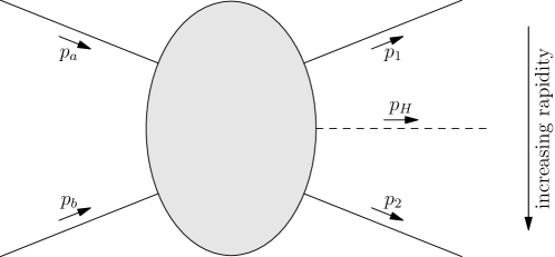
Figure 1: Production of a Higgs boson with momentum $p_{H}$ in between two jets with momenta $p_{1},p_{2}$. Arrows indicate the direction of the momentum flow.

Consider for illustration the production of a Higgs boson in association with dijets, with the rapidity of the Higgs boson between that of the jets. We label final momenta as shown in Fig. 1, such that the rapidities satisfy $y_{1}<y_{H}<y_{2}$ and the incoming momentum $p_{a}$($p_{b}$) is in the backward (forward) direction. In the following, we will be frequently interested in amplitudes in the limit of Multi-Regge kinematics (MRK), defined by a large center-of-mass energy $\sqrt{s_{12}}$, large invariant masses between all outgoing momenta, and fixed $t$-channel momenta. For our current example, we introduce the $t$-channel momenta of the system as $t_{1}=(p_{a}-p_{1})^{2},t_{2}=(p_{a}-p_{1}-p_{H})^{2}$ and consider large $s_{1H},s_{2H},s_{12}$, keeping $t_{1}$ and $t_{2}$ fixed. An analysis of the analytic properties of scattering amplitudes [38] (e.g. from Regge theory for multi-particle production) indicates that in this limit the on-shell scattering amplitude $\mathcal{M}$ should scale as [39]

$$\mathcal{M}\sim\ s_{1H}^{\alpha_{1}(t_{1})}\ s_{2H}^{\alpha_{2}(t_{2})}\ \gamma\left(t_{1},t_{2},s_{12}/(s_{1H}s_{2H})\right).$$ (1)

Here, $\alpha_{1}(t_{1})$ is the spin of the particle that can be exchanged in the $t_{1}$-channel between the particle of jet 1 and the Higgs boson, $\alpha_{2}(t_{2})$ is the equivalent for the $t_{2}$-channel between the Higgs boson and the particle of jet 2 and $\gamma$ is a function of transverse scales only. For a given momentum configuration of the jets and the Higgs boson, the leading contribution to $Hjj$-production therefore comes from the subprocesses with a parton flavour assignment to the jets which allows for the particle of the largest possible spin to be connecting the jets. For QCD this is the spin-1 gluonic colour-octet exchange. If the flavour assignment of a sub-process is such that a quark exchange is mandated, then the contribution to the jet cross section (proportional to the square of the matrix element) from this subprocess is suppressed by the invariant mass of the dijet pair, as compared to the subprocess where a gluon exchange is possible. For a given momentum configuration of the jets, the flavour assignments of the incoming states and of the corresponding jets which can proceed through gluon (colour-octet) exchanges between each jet are called the Fadin-Kuraev-Lipatov (FKL) configurations. These will form the leading contribution in $s_{ij}/t_{k}$ to the given jet configuration.

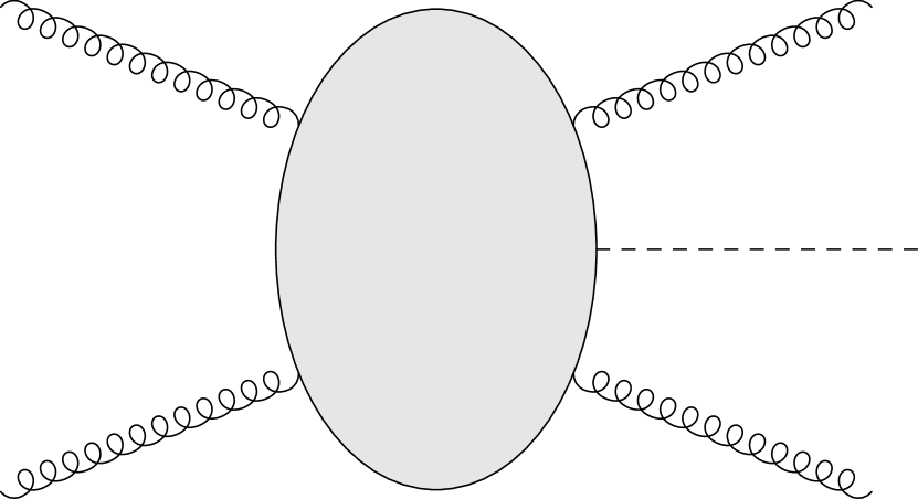
(a)

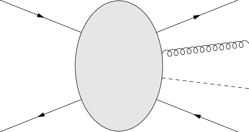
(b)

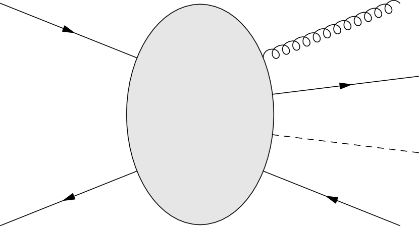
(c)

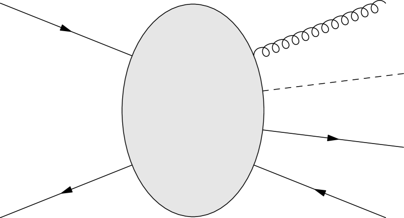
(d)

Figure 2: Example configurations for Higgs production in association with jets. Outgoing particles are ordered in increasing rapidity. Both (a) and (b) can be generated via gluonic $t$-channel exchange between each pair of adjacent outgoing particles and are therefore FKL configurations. The non-FKL configurations (c) and (d) require a quark $t$-channel exchange.

We illustrate this by continuing the example above. Consider first the case where both the incoming and the outgoing partons making up the jets are gluons as shown in Fig. 2(a). At Born level, the spin of all exchanged particles is 1 (since they are all gluons), and therefore the amplitude must scale as $\mathcal{M}\sim s_{1H}\ s_{2H}\ \gamma\left(t_{1},t_{2},s_{12}/(s_{1H}s_{2H})\right)$, where in the MRK limit $s_{12}/(s_{1H}s_{2H})\to 1/(m_{H}^{2}+p_{\perp H}^{2}),t_{1}\to-p^{2}_{\perp j_{1}},t_{2}\to-p^{2}_{\perp j_{2}}$, such that $\gamma$ depends on transverse scales only. This scaling is indeed demonstrated in Fig. 3. This plot shows $\overline{|\mathcal{M}|}^{2}/(s_{1H}^{2}\ s_{2H}^{2})m_{\perp H}^{4}$, where the square of the Born level matrix element (extracted from Madgraph5_aMC@NLO[40]) is evaluated in the phase space configurations of increasing rapidity separation between all particles. In particular, the 4-momenta $p=(E,p_{x},p_{y},p_{z})$ of the two jets $p_{j_{1}},p_{j_{2}}$ and the Higgs boson $p_{H}$ are parametrised in terms of their transverse momenta, azimuthal angle and rapidity as

$$\begin{split}p_{j_{1}}&=p_{\perp 1}(\cosh y_{1},\cos\phi_{1},\sin\phi_{1},\sinh y_{1})\\ p_{j_{H}}&=(m_{\perp H}\cosh y_{H},p_{\perp H}\cos\phi_{H},p_{\perp H}\sin\phi_{H},m_{\perp H}\sinh y_{H})\\ p_{j_{2}}&=p_{\perp 2}(\cosh y_{2},\cos\phi_{2},\sin\phi_{2},\sinh y_{2}).\end{split}$$ (2)

The specific choices for angles and transverse momenta are irrelevant for the conclusion, but here the phase space points used in the plot were $p_{\perp 1}=p_{\perp 2}=70$ GeV, $\phi_{1}=\frac{2}{3}\pi$, $y_{1}=-\Delta$, $\phi_{2}=\pi$, $y_{2}=\Delta$, $y_{H}=\Delta/3$ and $p_{\perp H}=-(p_{\perp 1}+p_{\perp 2})$ where $\Delta$ is increasing along the $x$-axis. The matrix element exhibits the expected Multi-Regge scaling according to Eq. (1), for spin-1 (gluon) exchanges, as $\overline{|\mathcal{M}|}^{2}/(s_{1H}^{2}\ s_{2H}^{2})m_{\perp H}^{4}$ tends to a constant as $\Delta y$ increases.

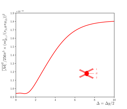
Figure 3: The square of the partonic matrix element for the processes $gg\to gHg$ divided by $(s_{j_{1}H}^{2}\ s_{j_{2}H}^{2})m_{\perp H}^{4}$. This is plotted for the phase space points parametrised according to Eq. (2). The square of the matrix element exhibits the expected Multi-Regge scaling according to Eq. (1), for spin-1 (gluon) exchanges and $\gamma\propto 1/m_{\perp H}^{4}$, as the curve tends to a constant for increasing $\Delta y$.

We can illustrate the suppression introduced when one requires a quark exchange in the $t$-channel by considering the squared matrix-elements for non-FKL configurations versus a corresponding FKL configuration. We will consider the three rapidity orderings of the flavour content in the process $pp\to Hj_{1}j_{2}j_{3}$ shown in panels (b) to (d) of Fig. 2. The rapidity-ordering $qQ\to qgHQ$ can proceed through colour-octet exchanges between each of the jet-pairs $(j_{1},j_{2})$, and $(j_{2},j_{3})$ (and the Higgs boson) and hence is an FKL configuration. The square of the matrix element for the cross section then scales as $|\mathcal{M}_{1}|^{2}\propto s_{j_{1}j_{2}}^{2}s_{j_{2}H}^{2}s_{Hj_{3}}^{2}\Gamma_{1}$ (where $\Gamma_{1}$ depends on transverse scales only). If now the parton content of $j_{1}$ and $j_{2}$ is swapped, the previous possibility of a gluon exchange between jets 1 and 2 is replaced by a quark exchange. Therefore, the scattering-process will scale as $|\mathcal{M}_{2}|^{2}\propto s_{j_{1}j_{2}}s_{j_{2}H}^{2}s_{Hj_{3}}^{2}\Gamma_{2}$ (where $\Gamma_{2}$ depends on transverse scales only), which is therefore suppressed by one power of $s_{j_{1}j_{2}}$ with respect to the FKL configuration. The third configuration we consider is $qQ\to gHqQ$. Like the second configuration, this only allows a quark exchange between jets 1 and 2, now with the Higgs boson in between in rapidity, and hence scales as $|\mathcal{M}_{3}|^{2}\propto s_{j_{1}H}s_{Hj_{2}}s_{j_{2}j_{3}}^{2}\Gamma_{3}$ (where $\Gamma_{3}$ depends on transverse scales only).

We illustrate the behaviour of these matrix elements in Fig. 4. The left plot clearly shows the resulting suppression of the square of the matrix elements for the non-FKL configurations ($qQ\to gqHQ$ (blue) and $qQ\to gHqQ$ (green)) compared to the FKL ordering $qQ\to qgHQ$ (red). The latter tends to a constant times $s^{2}$ while the first two exhibit an exponential suppression for large $\Delta y$ (corresponding to a power-suppression in $s_{j_{1}j_{2}}$). The suppression is indeed verified to be $s_{j_{1}j_{2}}$ on the right-hand plot in Fig. 4. Here, the squared matrix elements $|\mathcal{M}|^{2}$ divided by $s^{2}$ has been multiplied by $s_{j_{1}j_{2}}$ and tends to a constant for large $\Delta y$ in both cases.

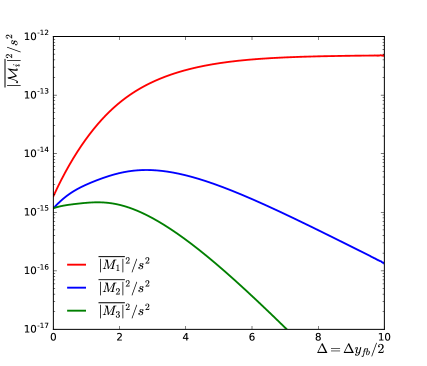
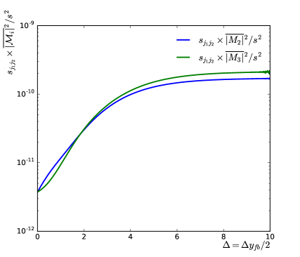
Figure 4: These plots demonstrate that introducing a quark exchange in place of a gluon exchange does indeed suppress the amplitude compared to the FKL configuration. In the left plot, the squared matrix elements are shown divided by $s^{2}$ for the three rapidity configurations described in the text. For the FKL configuration, $\overline{|M_{1}|}^{2}/s^{2}$ (red) tends to a constant as the rapidity separation increases, while the same quantity for the non-FKL configurations $\overline{|M_{2}|}^{2}$ (blue) and $\overline{|M_{3}|}^{2}$ (green) are exponentially suppressed. In the right plot, the suppression is shown to be a factor of $s_{j_{1}j_{2}}$ as the same quantities multiplied by $s_{j_{1}j_{2}}$ now tend to a constant in agreement with Eq. (1) .

2.1.2 Leading Contribution from Perturbative QCD

An alternative derivation of the dominance of the FKL configurations can be found by considering which of all the possible colour connections will dominate in the Multi-Regge-Kinematic (MRK) limit. As the Higgs boson is colour-neutral and irrelevant for the arguments, we restrict here the discussion to amplitudes involving just quarks and gluons, and follow the treatment of Ref. [41]. We begin by considering the process $qg\to qg$. Without loss of generality we take the backward incoming parton to be the quark. For the outgoing quark and gluon, there are obviously two possible rapidity-orderings : $y_{q}<y_{g}$ and $y_{q}>y_{g}$. These are shown in diagrams with rapidity-ordered final states in Figs. 5 and 6, together with the corresponding planar colour connections.

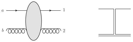
Figure 5: Left: Quark-gluon scattering with rapidity ordering $y_{q}\ll y_{g}$ and Right: The corresponding leading colour connection in the MRK limit.

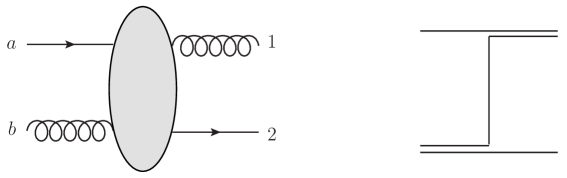
Figure 6: Left: Quark-gluon scattering with rapidity ordering $y_{q}\gg y_{g}$ and Right: The corresponding leading colour connection in the MRK limit.

By explicit calculation one quickly finds (see appendix A) that the tree-level result for the initial states fixed as the gluon incoming with positive light-cone momentum and the quark with negative light-cone momentum, the amplitude for the two rapidity orderings of the final state in the MRK limit scale as

$$|\mathcal{M}(y_{q}\ll y_{g})|\sim s\ \gamma_{1}\ \quad{\rm and}\quad|\mathcal{M}(y_{q}\gg y_{g})|\sim\sqrt{s}\ \gamma_{2},$$ (3)

in agreement with Eq. (1) and hence the dominant flavour-configuration in the MRK limit is given by the momentum configuration with $y_{q}\ll y_{g}$. As illustrated in the figures, this is the configuration where a colour octet (two colour lines) is exchanged, when particles are drawn ordered in rapidity.

2.1.3 Dominant Contributions at Arbitrary Multiplicities

The result of the previous section in fact generalises beyond the simple $2\to 2$ process. In Ref. [41], the compact Parke-Taylor expression[42] for the maximally helicity violating (MHV) amplitudes for all-gluon processes $gg\to g...g$ was used to show that for an arbitrary number of gluons, the colour connections which dominate kinematically in the MRK limit are those which can be represented on a so-called two-sided plot. An example of such a plot is shown in Fig. 7. The momentum of the incoming particles are labelled $p_{a}$ (negative $z$-momentum), and $p_{b}$ (positive $z$-momentum), and the outgoing particles are ordered in rapidity from left to right.

The colour connections which dominate in the MRK limit are found[41] to be precisely all those which may be drawn without any crossed lines. Furthermore, these colour connections all contribute with the same kinematic factor in the MRK limit.

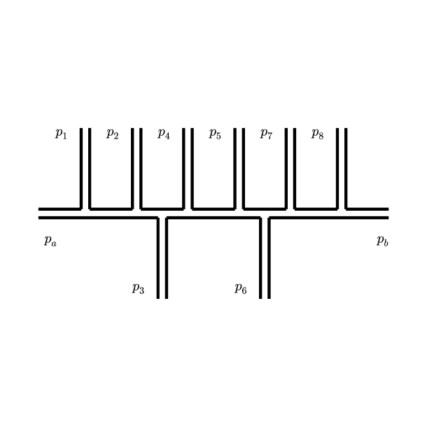
Figure 7: Parke-Taylor amplitude with colour ordering which respects the rapidity ordering $y_{1}\ll\cdots\ll y_{8}$.

The colour factor arising from these planar colour connections coincides with the colour factor from a single diagram with maximal t-channel gluon exchanges. In other words, for $2\to n$ gluons, the single colour factor of the FKL amplitude would be

$$f^{c_{a}c_{1}d_{1}}f^{d_{1}c_{2}d_{2}}...f^{d_{n-1}c_{n}c_{b}},$$ (4)

where $c_{a}$, $c_{1}$, … are the colour indices of the rapidity-ordered external gluons and the $d_{i}$ are the repeated indices of t-channel gluons. All other independent permutations of the indices multiply kinematic factors which are suppressed in the MRK limit. The final result for the limit of the colour summed-and-averaged square of the scattering amplitude agrees with that of the high-energy limit of QCD derived by Fadin-Kuraev-Lipatov (FKL)[26].

The multi-Regge kinematic limit of the kinematic part of the Parke-Taylor amplitudes is found[43] to be such that the full colour summed and averaged square of the scattering amplitude receives a factor

$$\frac{4g^{2}C_{\!A}}{k_{i,\perp}^{2}}$$ (5)

for each final state gluon beyond the first two. For example, the MRK limit of the colour and spin summed and averaged matrix element for $gg\to gg$ is

$$\overline{\left|\mathcal{M}\right|^{2}}\longrightarrow\frac{4\hat{s}^{2}}{\left(N_{\!C}^{2}-1\right)}\ \frac{g^{2}C_{\!A}}{k_{1\perp}^{2}}\ \frac{g^{2}C_{\!A}}{k_{2\perp}^{2}}.$$ (6)

Similarly, the MRK limit of the colour and spin summed and averaged matrix element for $gg\to ggg$ is

$$\overline{\left|\mathcal{M}\right|^{2}}\longrightarrow\frac{4\hat{s}^{2}}{\left(N_{\!C}^{2}-1\right)}\ \frac{g^{2}C_{\!A}}{k_{1\perp}^{2}}\ \frac{4g^{2}C_{\!A}}{k_{2\perp}^{2}}\frac{g^{2}C_{\!A}}{k_{3\perp}^{2}}.$$ (7)

Up to this multiplicity, only MHV configurations contribute to the amplitude. The above expressions Eqs. (6) and (7) therefore already cover the most general case.

In the following, we consider the partons extremal in rapidity (i.e. partons 1 and 2 for the Born process, 1 and 3 for the $2\to 3$-scattering and 1 and $n$ in the general $2\to n$-scattering) to be hard in the perturbative sense. Additional partons emitted in-between in rapidity are then considered part of the radiative corrections to the process.

For a specific choice of rapidities for the extremal partons $p_{1},p_{3}$ in the limit of the $2\to 3$-matrix element of Eq. (7), the phase space integration of the position of the middle parton will contribute a factor

$$\int\frac{\mathrm{d^{2}}k_{2\perp}}{(2\pi)^{2}}\int_{y_{1}}^{y_{3}}\ \frac{dy_{2}}{4\pi}\frac{4g^{2}C_{\!A}}{k_{2\perp}^{2}}=\frac{y_{3}-y_{1}}{4\pi}\int\frac{\mathrm{d^{2}}k_{2\perp}}{(2\pi)^{2}}\frac{4g^{2}C_{\!A}}{k_{2\perp}^{2}}=(y_{3}-y_{1})\ 4\alpha_{s}C_{\!A}\ \int\frac{\mathrm{d^{2}}k_{2\perp}}{(2\pi)^{2}}\frac{1}{k_{2\perp}^{2}}.$$ (8)

The integral over transverse phase space is IR divergent; the divergence cancels that introduced by the virtual corrections to the $2\to 2$-scattering. This cancellation is organised by using e.g. dimensional regularisation of the integrals, as will be discussed in more detail later. The point here is that the real (and virtual) corrections to the Born-level scattering introduce corrections proportional to the rapidity separation between the extremal (Born-level) partons. In the MRK limit, $\log\hat{s}/\hat{t}\to(y_{3}-y_{1})$, and so we have sketched the appearance of logarithmic corrections in the perturbative series of the $2\to 2$-scattering.

This analysis carries through to any order in $\alpha_{s}$. One notes that all dependence on the rapidity of the middle partons is absent in the factor in Eq. (5), and in the contribution to the corrections of Eq. (8) . This leads to a simple diffential equation for the cross section in $\Delta y=y_{n}-y_{1}$; this is called the BFKL evolution equation[26, 27, 28].

Above, we have discussed the colour connections present in the MRK limit in the tree-level matrix elements for any number of final-state gluons, i.e. the real corrections to the Born level. The virtual corrections are encoded at all-orders through simple factors multiplying the $t$-channel poles and hence the colour discussion above generalises immediately to these cases too.

At higher multiplicities, also non-MHV configurations contribute to the amplitude. In the MRK limit, the dominant configurations all conserve helicity between the incoming gluon and the extremal gluon at the respective end (for MHV configurations, this can be seen directly by considering the numerators in the Parke-Taylor amplitudes [41]). Flipping the helicity of any gluon emitted in-between the extremal gluons only changes the matrix element by a phase in the MRK limit, so that all helicity configurations which occur in the MRK limit can be related to the Parke-Taylor formula.

2.2 Fadin-Kuraev-Lipatov Amplitudes

In the previous section, we described the behaviour of QCD amplitudes in the limit of large invariant mass between each particle. Obviously, if the full amplitude is known, the MRK limit of it can be directly obtained. However, the limits can also be derived based on the Fadin-Kuraev-Lipatov (FKL) amplitudes[25, 26, 27].

QCD scattering amplitudes factorise in the MRK limit into what in the (B)FKL language are called impact factors and Lipatov vertices, which are connected by gluon exchanges in the t-channel. Each of these components of the amplitude depends only on a much reduced subset of momenta and is otherwise independent of the rest of the amplitude. This feature persists after the addition of a Higgs, $W$ or $Z/\gamma^{*}$ boson to the scattering. Two simple examples are shown in Fig. 8.

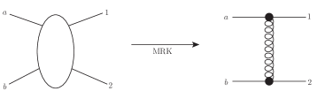
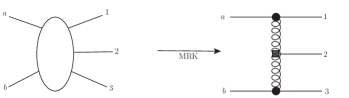
Figure 8: Two simple examples of the factorisation of QCD amplitudes in the MRK limit. Given the process described by the large oval on the left hand side, the amplitude in the MRK limit may be written as Left: a product of two independent impact factors (black circles) and a gluon exchange and, Right: two independent impact factors and a Lipatov emission vertex (grey square) connected with two t-channel gluon exchanges.

What is meant by the term “factorisation of the amplitude” is that the correct MRK limit of the amplitude can be obtained from a simple analytic approximation, which consists of factors, each of which depend only on a subset of all the momenta of the process. As an example, in the process on the left-hand-side of Fig. 8, the flavour $f_{1},f_{2}$ of the external lines may be quark or gluon and in the MRK limit ($y_{1}\ll y_{2}$), the amplitude may be expressed in the form:

$$\mathcal{M}_{f_{1}(p_{a})f_{2}(p_{b})\to f_{1}(p_{1})f_{2}(p_{2})}\to\hat{s}\ C(p_{a},p_{1})\ \frac{1}{(p_{a}-p_{1})^{2}}\ C(p_{b},p_{2}),$$ (9)

where $C(p_{i},p_{j})$ indicates an impact factor, which depends on the two momenta along the same direction on the light-cone only (i.e. $p_{a},p_{1}$ are the parton momenta each with the maximum positive light-cone momentum, $p_{b},p_{2}$ have the largest negative light-cone momentum). The correct MRK limit of the full amplitude would then be obtained with this analytic expression, for any configurations of the transverse momenta. The square of the amplitude is then simply found as

$$|\mathcal{M}_{f_{1}(p_{a})f_{2}(p_{b})\to f_{1}(p_{1})f_{2}(p_{2})}|^{2}\to\hat{s}^{2}\ \frac{|C(p_{a},p_{1})|^{2}}{(p_{a}-p_{1})^{2}}\ \frac{|C(p_{b},p_{2})|^{2}}{(p_{b}-p_{2})^{2}}.$$ (10)

Similarly, the correct MRK limit of the scattering amplitude for the three-particle final state on the right-hand side may be written

$$\begin{split}|\mathcal{M}_{f_{1}(p_{a})f_{2}(p_{b})\to f_{1}(p_{1})g(p_{2})f_{2}(p_{3})}|^{2}&\to\hat{s}^{2}\frac{|C(p_{a},p_{1})|^{2}}{(p_{a}-p_{1})^{2}}\frac{|V_{L}(p_{2})|^{2}}{(p_{a}-p_{1})^{2}(p_{b}-p_{3})^{2}}\frac{|C(p_{b},p_{3})|^{2}}{(p_{b}-p_{3})^{2}}\\ &=\hat{s}^{2}\frac{|C(p_{a},p_{1})|^{2}}{t_{1}}\frac{|V_{L}(p_{2})|^{2}}{t_{1}\ t_{2}}\frac{|C(p_{b},p_{3})|^{2}}{t_{2}}\end{split}$$ (11)

where $V_{L}$ is a so-called Lipatov vertex. The only difference to the form of the two-particle final state is the insertion of a vertex and a propagator in the analytic form of the MRK limit, which has a form suggestive of the $t$-channel exchange. The $t$-channel interpretation of the analytic form of the kinematic part of the amplitude is supported by the colour-connections studied in Sec. 2.1.2, but while the contribution from individual $t$-channel Feynman diagrams are obviously gauge dependent, it is important to realise that the MRK limit of the scattering amplitude is a gauge-independent statement. It just happens to have the analytic form expected from a $t$-channel gluon exchange, as expected from the analysis presented in Sec. 2.1.1.

For the impact factors one finds $|C(p_{a},p_{1})|^{2}=1$, and in the MRK limit $t_{1}\to-k_{1\perp}^{2},t_{2}\to-k_{3\perp}^{2}$, and one finds[27] that the factor introduced from an additional gluon emission of transverse momentum $k_{2\perp}$ into the FKL result for the square of the matrix element is simply

$$\frac{|V_{L}(p_{2})|^{2}}{t_{1}\ t_{2}}\to\frac{4g^{2}C_{\!A}}{k_{2\perp}^{2}}.$$ (12)

Therefore, the MRK limit of the QCD amplitudes found in Sec. 2.1.3 are reproduced by the FKL amplitudes[43, 41]. This is true for an arbitrary number of gluons emitted, such that the FKL result for the leading-order contribution to the colour-and-spin summed-and-averaged square of the scattering amplitude is given by

$$\overline{|\mathcal{M}^{\mathrm{FKL}}_{gg\to g_{1}\cdots g_{n}}|^{2}}=\frac{2\hat{s}^{2}}{4\left(N_{\!C}^{2}-1\right)}\prod_{1}^{n}\frac{g^{2}C_{\!A}}{k_{i\perp}^{2}}.$$ (13)

The $t$-channel structure of the FKL amplitudes allows for the inclusion of the dimensionally regulated virtual corrections (in $D=4-2\varepsilon$ dimensions) through the Lipatov Ansatz for the Reggeized $t$-channel colour-octet exchanges. This is the prescription for including the all-order virtual corrections to the Born-level colour octet exchange by making the following substitution in Eq. (10):

$$\frac{1}{t_{i-1}}\ \to\ \frac{1}{t_{i-1}}\ \exp\left[\hat{\alpha}(q_{i})(y_{i-1}-y_{i})\right]$$ (14)

where

$$\hat{\alpha}(q_{i}) =-g^{2}\ C_{\!A}\ \frac{\Gamma(1-\varepsilon)}{(4\pi)^{2+\varepsilon}}\frac{2}{\varepsilon}\left(q_{i\perp}^{2}/\mu^{2}\right)^{\varepsilon},$$ (15)

with $q_{i}=p_{a}-\sum_{j=1}^{i}p_{j}$, such that $t_{i}=q_{i}^{2}$. This ansatz for the exponentiation of the virtual corrections in the appropriate limit of the $n$-parton scattering amplitude has been proved to even the sub-leading level[44, 39, 45, 46], which leads to a perturbative correction to leading-logarithmic results for $\hat{\alpha}$, the Lipatov vertex and the impact factors.

The FKL result for the square of the scattering matrix for $2\to n$ obtained by using the kinematic approximations valid in the multi-regge-kinematic limit has no dependence on the rapidities of the final-state particles (in essence because the limit of infinite rapidity-separation has been applied). The poles in $\epsilon$ in the dimensionally regulated inclusion of the virtual corrections through the Lipatov ansatz turn out to cancel order-by-order with the poles from the dimensionally regulated integration over the soft phase space of additional emissions (intermediate in rapidity between parton 1 and $n$) included through the FKL result for the square of the matrix element for $2\to m,m>n$. A finite contribution from the virtual corrections is left over. If now the contribution to the centre-of-mass energy $\sqrt{\hat{s}}$ and therefore also to the longitudinal momentum of the incoming partons is ignored from all but the most backward and forward parton, then the sum over the integration over phase space of any parton of intermediate rapidity can be performed analytically. This leads to the much celebrated BFKL equation[28], which captures the leading (and sub-leading) behaviour in $\log(\hat{s}/p_{t}^{2})$. It is seen that the logarithmic behaviour is the same when using the FKL amplitudes of Eq. (13) and the limit of the full QCD amplitudes as discussed in Sec. 2.1.3. The large-rapidity behaviour of the $m$-parton amplitudes of full QCD and FKL is the same in terms of powers of $\hat{s}/p_{ti}^{2}$, which is sufficient to guarantee the same logarithmic behaviour of the integrated cross section in terms of $\log(\hat{s}/p_{t}^{2})$.

2.3 Construction of the Simplest HEJ Amplitude

In the previous two subsections, we have described how the leading behaviour of scattering amplitudes in QCD arises through the study of $t$-channel poles, and how the simple structure in the MRK limit is captured to all orders in $\alpha_{s}$ by the FKL amplitudes. So far with HEJ, all-order results have been achieved for such FKL configurations only. All other kinematic configurations have been included to fixed order only through a matching and merging procedure described in Sect. 2.7. In this paper, we present for the first time the inclusion of all-order results also for some sub-leading corrections, namely quark-initiated processes with one gluon emitted outside the FKL-ordered phase space. These configurations correspond to the suppressed contributions studied in Figure 4. The leading logarithmic corrections to these processes constitute the first sub-leading logarithmic corrections included in HEJ. The configurations constitute the largest part of the sub-leading cross-section, which previously was included through the naïve addition of fixed-order samples. The inclusion of these sub-leading (and their matching to fixed-order accuracy) therefore gives a much more satisfactory theoretical description of the scattering.

The motivation behind the HEJ framework is to capture the behaviour of amplitudes at large $\hat{s}$ without applying the full tower of approximations necessary for obtaining an analytic answer for the cross section through the BFKL theory. By allowing for numerical integration of multi-particle amplitudes, we can both allow these to have a more complicated kinematic dependence than the $1/k_{\perp}^{2}$ of the FKL-amplitudes, and account for the longitudinal momentum-conservation which is invariably lost in any formulation involving the BFKL equation (at both LL and NLL accuracy).

The simplest of all QCD processes is that of $qQ\to qQ$, proceeding through a $t$-channel gluon exchange only. The MRK limit of the full QCD result and the FKL approximation of the square of this amplitude is

$$\overline{|\mathcal{M}^{\mathrm{QCD}}_{qQ\to qQ}|^{2}}\to\overline{|\mathcal{M}^{\mathrm{FKL}}_{qQ\to qQ}|^{2}}=\frac{2\hat{s}^{2}}{4\left(N_{\!C}^{2}-1\right)}\frac{g^{2}C_{\!F}}{k_{1\perp}^{2}}\frac{g^{2}C_{\!F}}{k_{2\perp}^{2}}=\frac{\left(g^{2}C_{\!F}\right)^{2}}{4(N_{\!C}^{2}-1)}\frac{2\hat{s}^{2}}{k_{1\perp}^{2}k_{2\perp}^{2}}.$$ (16)

The leading-order QCD result is given by

$$\overline{|\mathcal{M}^{\mathrm{QCD}}_{qQ\to qQ}|^{2}}=\frac{\left(g^{2}C_{\!F}\right)^{2}}{4(N_{\!C}^{2}-1)}\frac{\hat{s}^{2}+\hat{u}^{2}}{\hat{t}^{2}}.$$ (17)

Two kinematic approximations are necessary to get from the full result to the approximation of FKL: $\hat{s}\sim-\hat{u}$, $\hat{t}\sim-k_{1\perp}^{2}=-k_{2\perp}^{2}$ (where the last equality holds for the simple $2\to 2$ process). While both of these are valid in the MRK limit, they are easily off by an order of magnitude within the relevant phase space of the LHC.

In constructing a Monte Carlo phase space integrator, which is sufficiently efficient to calculate explicitly the phase space integration over many-particle (e.g. up to 30) final state phase space, we can seek to build an approximation for the matrix elements, which still captures the leading logarithmic behaviour generated from the $t$-channel poles, but which relies on fewer kinematic approximations. In particular, we want the description of the amplitude to be:

• exact for the simple $2\to 2$-process proceeding only through a $t$-channel exchange;

• gauge-invariant for any additional gluon emitted, i.e. the Ward Identity is fulfilled (not just asymptotically in the MRK-limit, as for FKL-amplitudes, but exactly, everywhere in phase space), $k_{n}^{\mu}\mathcal{M}_{\mu}=0$;

• such that the soft divergences of the approximant are cancelled by the terms generated from the Lipatov Ansatz for the virtual corrections to the tree-level results (also for $2\to n$-processes); and

• sufficiently fast to evaluate such that the numerical integration is feasible.

Let us first focus on building this simple approximant for the $2\to 2$-processes. The Lipatov Ansatz can most easily be applied if the analytic structure of the $m$-parton amplitude is factorised into a dependence on $1$-parton and the $(m-1)$-parton amplitude (obviously evaluated with the momenta of the $m$-parton phase space). It is therefore important to build a good approximant to even the simplest processes, since obviously the multi-particle approximations are built on successive applications of these. We will see that by using helicity amplitudes, we can build such a simple structure for approximants of multi-particle amplitudes, which are valid even before the Multi-Regge-Kinematic limit is applied.

Since we will be evaluating the amplitudes numerically in the Monte-Carlo integration, there is no problem in keeping the full kinematic dependence on the $t$-channel propagator-momentum $\hat{t}$ in Eq. (17) rather than performing the MRK-approximation $\hat{t}\to-k_{1\perp}^{2}$. Clearly, the $t$-channel poles are described best by maintaining the full dependence on the $t$-channel momenta. We now turn to describing the remaining invariants, $s$ and $u$. In the full MRK limit, $s=-u$; in practice, there is a large deviation throughout phase space. By studying the amplitude for $qQ\to qQ$, we find that terms proportional to $s^{2}$ arise from amplitudes where the quarks have identical helicities; while terms proportional to $u^{2}$ arise from amplitudes where the two quark lines have opposite helicities. Explicitly, in terms of currents $j^{\mu\pm}(p_{i},p_{j})=\bar{u}^{\pm}(p_{i})\gamma^{\mu}u^{\pm}(p_{j})$, one finds that

$$|j^{\mu\pm}(p_{1},p_{a})\ j_{\mu}^{\pm}(p_{2},p_{b})|^{2}=s^{2},\quad|j^{\mu\pm}(p_{1},p_{a})\ j^{\mp}_{\mu}(p_{2},p_{b})|^{2}=u^{2}.$$ (18)

By working at the helicity amplitude level, we have achieved a description of the $2\to 2$ amplitude that is exact, and furthermore the analytic form generalises easily to $2\to n$. These components then depend on $\{p_{a},p_{1}\}$ and $\{p_{b},p_{2}\}$ separately as in Eq. (9). Hence the product of two scalar impact factors has been expanded to a contraction of vector currents.

In fact, this factorised form also continues when one moves to $qg\to qg$ with the same quark current as above [31]. The gluon current has an additional scalar factor, but it can still be written in a form which depends only on the gluon momenta, and can be found in Eq. (8) of Ref.[32], with the exact amplitude for $qg\to qg$ written in terms of the HEJ building-blocks as

$$\begin{split}|\mathcal{M}_{q^{-}g^{+}\to q^{-}g^{+}}|^{2}\ &=\frac{1}{N_{\!C}^{2}-1}\ |\langle\mskip-1.0mu{b}|\rho|{2}\mskip-1.0mu\rangle\langle\mskip-1.0mu{1}|\rho|{a}\mskip-1.0mu\rangle|^{2}\\ &\cdot\left(g_{s}^{2}\ C_{\!F}\ \frac{1}{t_{1}}\right)\\ &\cdot\left(g_{s}^{2}\ \left[\frac{1}{2}\ \frac{1+z^{2}}{z}\ \left(C_{A}-\frac{1}{C_{A}}\right)+\frac{1}{C_{A}}\right]\ \frac{1}{t_{2}}\right),\end{split}$$ (19)

where $z=p_{2}^{-}/p_{b}^{-}$ (and again $t_{1}=(p_{a}-p_{1})^{2}=(p_{b}-p_{2})^{2}=t_{2}$). This is written for the case of a backward moving incoming gluon; for a forward-moving gluon, one would simply define $z=p_{2}^{+}/p_{b}^{+}$. A similar $t$-channel factorised form is found for $g^{+}g^{-}\to g^{+}g^{-}$ scattering (in the configuration with scattering of gluons with the same helicity there is of course no unique concept of the $t$-channel).

We will later discuss how the scattering amplitude can be extended to capture the all-order leading logarithmic accuracy of the cross section by accounting for the emissions of additional gluons.

The structure of an amplitude approximated by building blocks, each depending only on the momenta of a small subset of the particles is obviously appealing computationally. Not only though are these factors independent of other particle momenta, they are completely independent of the rest of the process and are therefore in that sense, process-independent. So, if particles $a$ and $1$ are the same flavour in each case (either quark or gluon), the factor of the FKL formalism $C(p_{a},p_{1})$ in Eqs. (9) and (11) will be identical, and so will the currents used in HEJ.

The next building block we need to derive is the Lipatov vertex, $V_{L}$, for additional FKL-ordered gluon emissions. The simplest process to study is $qQ\to qgQ$. It is necessary to sum the contributions from all five tree-level diagrams. After some manipulation in the high-energy limit this yields[30]

$$\begin{split}\mathcal{M}^{\rm HEJ}_{\rm tree\ qQ\to qgQ}&=-g_{s}^{2}T^{a_{1}}_{i_{1}i_{a}}T^{a_{2}}_{i_{3}i_{b}}\ \frac{\mathcal{S}_{qQ}(p_{1},p_{3},p_{a},p_{b})}{q_{1}^{2}q_{2}^{2}}\times ig_{s}f^{a_{1}b_{2}a_{2}}\ \varepsilon_{\nu_{2}}(p_{2})V^{\nu_{2}}_{L}(q_{1},q_{2}),\end{split}$$ (20)

where $\mathcal{S}_{qQ}(p_{1},p_{3},p_{a},p_{b})$ is still a contraction of currents:

$$\mathcal{S}_{qQ}(p_{1},p_{3},p_{a},p_{b})=j^{\mu}(p_{1},p_{a})\ j_{\mu}(p_{3},p_{b}),$$ (21)

and $V^{\nu}_{L}$ is a Lipatov-type vertex for gluon emission, which is given by:

$$\begin{split}V_{L}^{\nu}(q_{i},q_{i+1})=&-(q_{i}+q_{i+1})^{\nu}\\ &+\frac{p_{a}^{\nu}}{2}\left(\frac{q_{i}^{2}}{p_{i+1}\cdot p_{a}}+\frac{p_{i+1}\cdot p_{b}}{p_{a}\cdot p_{b}}+\frac{p_{i+1}\cdot p_{n}}{p_{a}\cdot p_{n}}\right)+p_{a}\leftrightarrow p_{1}\\ &-\frac{p_{b}^{\nu}}{2}\left(\frac{q_{i+1}^{2}}{p_{i+1}\cdot p_{b}}+\frac{p_{i+1}\cdot p_{a}}{p_{b}\cdot p_{a}}+\frac{p_{i+1}\cdot p_{1}}{p_{b}\cdot p_{1}}\right)-p_{b}\leftrightarrow p_{n}.\end{split}$$ (22)

This form is slightly more involved than the standard Lipatov (or Reggeon-Reggeon-particle-) vertex of BFKL[47], since it maintains the dependence on each of the 4 quark momenta rather than making the approximation $p_{a}\sim p_{1},p_{b}\sim p_{n}$; the two last terms in each bracket constitutes the eikonal approximation to the emission off each leg. The difference between the form used in BFKL and in HEJ is formally sub-leading, but crucial for obtaining analytic results in BFKL. Conversely, the full form of Eq. (22) unsurprisingly gives a more accurate description of the sub-asymptotic region of phase space, and thus leads to smaller matching-corrections. In choosing to perform the phase space integrations numerically, we are free to choose the numerically more accurate form.

Now the power of the high-energy limit becomes manifest. With only the building blocks derived so far, the leading contribution of the scattering amplitude (in powers of $\hat{s}/p_{t}^{2}$, forming the leading logarithmic contribution to the integrated cross section) for any number of intermediate gluon emissions is described by

$$\begin{split}\mathcal{M}^{\rm HEJ}_{\rm tree}&=-g_{s}^{2}T^{a_{1}}_{i_{1}i_{a}}T^{a_{n-1}}_{i_{n}i_{b}}\ \frac{\mathcal{S}_{qQ}(p_{1},p_{n},p_{a},p_{b})}{\sqrt{q_{1}^{2}q_{j}^{2}q_{j+1}^{2}q_{n-1}^{2}}}\times\prod_{k=2}^{n-1}ig_{s}f^{a_{k-1}b_{k}a_{k}}\ \frac{\varepsilon_{\nu_{k}}(p_{k})V^{\nu_{k}}_{L}(q_{k-1},q_{k})}{\sqrt{q_{k-1}^{2}q_{k}^{2}}}.\end{split}$$ (23)

This structure is shown in Fig. 9, where the Lipatov vertices are shown as grey boxes. The amplitude for the equivalent process with one or two incoming gluons is identical, except for a minor alteration to the function $\mathcal{S}$.

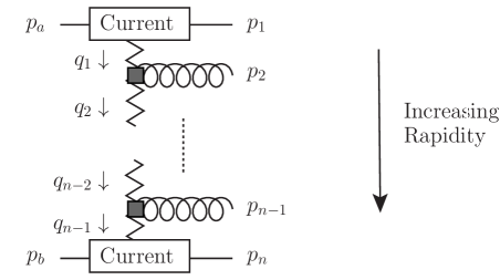
Figure 9: The analytic structure of the base tree-level scattering amplitude for $qQ\to qQ+(n-2)g$ in High Energy Jets. Grey boxes denote Lipatov vertices.

2.4 Regularisation and Leading Logarithmic All-Order Cross Sections

In sections 2.1–2.3 we identified the leading contributions for jet production in the multi-Regge-kinematic limit, and showed how to obtain an accurate approximation to the Born-level matrix elements for such processes for any multiplicity of gluon emissions. The only singularities present in this approximation are those arising from the $t$-channel propagators in the colour-octet exchanges of the rapidity-ordered final state, and these singularities of the Born-level amplitude are outside the physical region. As discussed in Section 2.1.3, logarithmic corrections in $\hat{s}/p_{t}^{2}$ arise in the region of jets widely separated in rapidity. So far, we have discussed Born-level results only. In this section, we will discuss the calculation of the cross section to each order in $\alpha_{s}$, and the regularisation of the IR singularities. No UV singularities appear at the logarithmic order discussed.

The reason for developing an approximation to the $t$-channel poles of the scattering tree-level matrix elements is that the leading logarithmic contribution to the loop corrections of these processes can still be obtained using the Lipatov ansatz[26], just as discussed for the FKL amplitudes in Section 2.2. This ansatz states that the leading logarithmic contribution to the virtual corrections for amplitudes in the MRK limit can be found to all orders in the coupling by replacing each $t$-channel propagator between the two particles of ordered rapidities $y_{i}$ and $y_{i+1}$ ($y_{i}<y_{i+1}$) in the amplitudes constructed in section 2.3 as follows:-

$$\frac{1}{t_{i}}\ \to\ \frac{1}{t_{i}}\ \exp\left[\hat{\alpha}(q_{i})(y_{i+1}-y_{i})\right]$$ (24)

with

$$\hat{\alpha}(q_{i}) =-g^{2}\ C_{\!A}\ \frac{\Gamma(1-\varepsilon)}{(4\pi)^{2+\varepsilon}}\frac{2}{\varepsilon}\left(q_{i\perp}^{2}/\mu^{2}\right)^{\varepsilon}.$$ (25)

As mentioned earlier, this ansatz for the exponentiation and factorisation of the virtual corrections in the appropriate limit of the $n$-parton scattering amplitude has been proved to hold even at the sub-leading level [44, 39, 45, 46] and explicitly checked against the two-loop amplitudes for $qg$-scattering[48].

As demonstrated in e.g. Ref.[32] and below, the poles in $\epsilon$ cancel exactly between the dimensionally regularised (in $D=4-2\epsilon$ dimensions) virtual and real corrections to processes of any multiplicity, when calculated with the constructed amplitudes which ensure the correct leading logarithmic (in $\hat{s}$) behaviour of the cross section. This allows for the calculation of the inclusive cross section (for the leading and the included sub-leading processes) as explicit sums of $n$-body 4-dimensional phase space integrals of dimensionally regularised $n+2$-particle matrix elements.

The first step in organising the cancellation of the poles in $\varepsilon$ and obtaining the regularised cross sections is to define for each Born-level momentum configuration the regions in phase space for which the real corrections for gluon emissions can be calculated to any order in the coupling. It is the phase space region in rapidity delimited by the extremal partons. These partons extremal in rapidity are required to be perturbative (i.e. of a transverse momentum similar to the hard jet scale), since these form parts of the fundamental currents of the formalism, and there is (at LL accuracy) no accompanying virtual corrections to regulate the divergences present as the transverse momenta of these extremal partons tend to zero. However, for the phase space bounded in rapidity by these extremal, hard partons, the soft singularity from the real emission of additional gluons is regulated by the singularity from the virtual corrections to all orders in the coupling (i.e. for any number of emissions into that region of rapidity).

To illustrate the specifics of this procedure, consider for simplicity the process $qQ\to jj$. We will now show how the leading logarithmic perturbative corrections to this process are calculated to all orders through the explicit construction of regulated, four-dimensional amplitudes, which can be summed and integrated explicitly using Monte-Carlo techniques.

We will apply dimensional regularisation (working in $D=4-2\varepsilon$ dimensions) in order to facilitate the cancellation of poles from real and virtual corrections. The colour and spin summed and averaged square of the scattering matrix element for the process $f_{1}f_{2}\to f_{1}\cdot g\cdot f_{2}$ (where $\cdot g\cdot$ indicates the possibility of any number of gluons), following from Eq. (23) but extended to $4-2\epsilon$ dimensions, is

$$\begin{split}\overline{\left|\mathcal{M}^{\rm HEJ}_{\varepsilon\ f_{1}f_{2}\to f_{1}\cdot g\cdot f_{2}}\right|}^{2}=\ &\frac{1}{4\ (N_{\!C}^{2}-1)}\ \left\|S_{f_{1}f_{2}\to f_{1}f_{2}}\right\|^{2}\\ &\cdot\ \left(g_{s}^{2}\ K_{f_{1}}\ \frac{1}{t_{1}}\right)\cdot\ \left(g_{s}^{2}\ K_{f_{2}}\ \frac{1}{t_{n-1}}\right)\\ &\cdot\prod_{i=1}^{n-2}\left(\frac{-g_{s}^{2}C_{A}}{t_{i}t_{i+1}}\ V^{\mu}(q_{i},q_{i+1})V_{\mu}(q_{i},q_{i+1})\right)\\ &\cdot\prod_{j=1}^{n-1}\exp\left[2\hat{\alpha}(q_{j})(y_{j+1}-y_{j})\right].\end{split}$$ (26)

The colour factors $K_{f_{i}}$ are $C_{F}$ if particle $i$ is a quark and $C_{A}$ if it is a gluon. The matrix element above describes the leading-logarithmic corrections to dijet production at all orders in $\alpha_{s}$. These take the form of additional partons in the final state described by the $V^{\mu}$ emission vertices and the corresponding exponential factors arising from the virtual contributions to the process. We organise the cancellation of the divergences by means of a phase-space slicing parameter $\lambda$, which separates the “hard” region ($p_{\perp}>\lambda$) from the “soft” region ($p_{\perp}<\lambda$). The divergences arising from soft emissions arise from the singularities of the emission vertices. Explicitly, in the limit that $p_{k}\to 0$,

$$\frac{V^{\mu}(q_{k-1},q_{k})V_{\mu}(q_{k-1},q_{k})}{t_{k-1}t_{k}}\to\frac{-4}{p_{k\perp}^{2}}.$$ (27)

We therefore have

$$\overline{\left|\mathcal{M}^{\rm HEJ}_{{\rm tree},\varepsilon\ f_{1}f_{2}\to f_{1}(n-2)gf_{2}}(\{p_{i}\})\right|}^{2}\quad\begin{array}[]{c}\longrightarrow\\ p_{k}\to 0\end{array}\quad\left(\frac{4g_{s}^{2}C_{A}}{p_{k\perp}^{2}}\right)\ \overline{\left|\mathcal{M}^{\rm HEJ}_{{\rm tree},\varepsilon\ f_{1}f_{2}\to f_{1}(n-3)gf_{2}}(\{p_{i}\}\backslash p_{k})\right|}^{2}.$$ (30)

The set of particle momenta on the right-hand side (the set of $n-1$ momenta obtained by removing $p_{k}$) still satisfies momentum conservation since we are precisely considering the case of $p_{k}\to 0$. The divergence in the $2\to n$-scattering matrix element in the limit $p_{k}\to 0$ is therefore identical to that obtained using the simple factor in Eq. (30). We can therefore organise the cancellation of soft divergences between real and virtual corrections by first subtracting the term in brackets from the square of the Lipatov vertices. Since we only need to regularise the divergence, we will restrict this real-subtraction term to soft momenta, i.e. $p_{k\perp}<\lambda$. The integral of the real-emission subtraction term is then found as

$$\begin{split}\mu^{-2\varepsilon}\int_{\rm soft}\frac{d^{3+2\varepsilon}p_{k}}{(2\pi)^{3+2\varepsilon}2E_{k}}\ \frac{4g_{s}^{2}C_{A}}{|p_{k\perp}|^{2}}&=\mu^{-2\varepsilon}\int_{0}^{\lambda}\frac{d^{2+2\varepsilon}p_{k\perp}}{(2\pi)^{2+2\varepsilon}}\int_{y_{k-1}}^{y_{k+1}}\frac{dy_{k}}{4\pi}\ \frac{4g_{s}^{2}C_{A}}{|p_{k\perp}|^{2}}\\ &=\mu^{-2\varepsilon}\frac{4g_{s}^{2}C_{A}}{(2\pi)^{2+2\varepsilon}(4\pi)}(y_{k+1}-y_{k-1})\int_{0}^{\lambda}\frac{d^{2+2\varepsilon}p_{k\perp}}{|p_{k\perp}|^{2}}\\ &=\frac{g_{s}^{2}C_{A}}{\pi(2\pi)^{2+2\varepsilon}}\ (y_{k+1}-y_{k-1})\ \frac{1}{\varepsilon}\frac{\pi^{1+\varepsilon}}{\Gamma(1+\varepsilon)}\left(\frac{\lambda^{2}}{\mu^{2}}\right)^{\varepsilon}.\end{split}$$ (31)

This contribution will be added to the virtual corrections for the $n-1$-momenta state. These virtual corrections can be found by expanding the exponential factor in the last line of Eq. (26) which spans the rapidity region integrated over in Eq. (31). We therefore find to first order in $\alpha_{s}$

$$\begin{split}\left(-2(y_{k+1}-y_{k-1})g_{s}^{2}C_{A}\frac{\Gamma(1-\varepsilon)}{(4\pi)^{2+\varepsilon}}\frac{2}{\varepsilon}\left(\frac{q_{k\perp}^{2}}{\mu^{2}}\right)^{\varepsilon}\right)\overline{\left|\mathcal{M}^{\rm HEJ}_{{\rm tree},\varepsilon\ f_{1}f_{2}\to f_{1}(n-3)gf_{2}}(\{p_{i}\}\backslash p_{k})\right|}^{2}.\end{split}$$ (32)

Combining this with the contribution from the integral of the real-emission subtraction term in Eq. (31) and expanding in $\varepsilon$, the pole in $\varepsilon$ and (the dependence on $\mu$) cancels exactly. This is in fact true order-by-order in $\varepsilon$, and the finite correction which remains can be absorbed into the regularised trajectory

$$\omega^{0}(q_{\perp}^{2}) =\frac{g_{s}^{2}C_{A}}{4\pi^{2}}\ \log\left(\frac{\lambda^{2}}{q_{\perp}^{2}}\right)=\alpha_{s}\frac{C_{A}}{\pi}\ \log\left(\frac{\lambda^{2}}{q_{\perp}^{2}}\right).$$ (33)

We can repeat this for each real emission between the extremal partons, which yields the following all-order description of dijet production:

$$\begin{split}\overline{\left|\mathcal{M}^{\rm HEJ}_{\varepsilon\ f_{1}f_{2}\to f_{1}\cdot g\cdot f_{2}}\right|}^{2}=\ &\frac{1}{4\ (N_{\!C}^{2}-1)}\ \left\|S_{f_{1}f_{2}\to f_{1}f_{2}}\right\|^{2}\\ &\cdot\ \left(g_{s}^{2}\ K_{f_{1}}\ \frac{1}{t_{1}}\right)\cdot\ \left(g_{s}^{2}\ K_{f_{2}}\ \frac{1}{t_{n-1}}\right)\\ &\cdot\prod_{i=1}^{n-2}\left(\frac{-g_{s}^{2}C_{A}}{t_{i}t_{i+1}}\ V^{\mu}(q_{i},q_{i+1})V_{\mu}(q_{i},q_{i+1})\right)\\ &\cdot\prod_{j=1}^{n-1}\exp\left[\omega^{0}(q_{j\perp})(y_{j+1}-y_{j})\right].\end{split}$$ (34)

The remaining numerical phase space integration now excludes the soft region, i.e. we require $p_{k\perp}>\lambda$ for all emitted gluons.

In practice, we find that the contribution from the small, finite integral of the difference between the Lipatov vertex and the subtraction term is negligible for transverse momenta less than roughly $\kappa=0.2$ GeV $=200$ MeV, but can be relevant if $\lambda$ is larger than that value. We therefore add the correction

$$\frac{V^{\mu}(q_{k-1},q_{k})V_{\mu}(q_{k-1},q_{k})}{t_{k-1}t_{k}}+\frac{4}{p_{k\perp}^{2}}.$$ (35)

for values of $\kappa<|p_{k\perp}|<\lambda$ and find stable results under variation of both $\kappa$ and $\lambda$. Numerically stable results can be obtained with $\kappa$ as low as 0.1 GeV (but we will take $\kappa=0.2$ GeV since the results are the same, but require less computing time). In fact, if we choose $\kappa=\lambda$, then the real subtraction term is only applied in the region of phase space which is integrated over analytically. In the remaining transverse-momentum phase space, which is integrated over numerically, the integrand will be positive definite, since the Lipatov vertex is a space-like 4-vector, and there are no subtraction terms in this resolved phase space.

The matrix-element squared in Eq. (34) is the basis of the HEJ description of dijet production. In order to generate final cross sections, this is supplemented with both matching and merging and is then integrated over the final phase space. However, this procedure will be the same after the inclusion of the new corrections described in the next section, and we therefore postpone the discussion of these final aspects until Section 2.7.

2.5 The First Set of Sub-Leading Corrections

Section 2.1 presented the FKL configurations, i.e. the flavour and momentum configurations which result in the leading power behaviour in $s/p_{\perp}^{2}$ of the amplitudes. By integrating these over phase space we find the leading logarithmic contributions in $s/p_{\perp}^{2}$ to the cross section. There is a term of order $\alpha_{s}\log(\hat{s}/t)\approx\alpha_{s}\Delta y$ contributing for each additional emission of a gluon between the two quarks in rapidity. These terms contribute to the cross section as $\alpha_{s}^{2}(\alpha_{s}\Delta y)^{n}$ for all $n$. The remaining momentum-orderings can be included by simply adding tree-level predictions for these to the events sample, as done in Ref.[32, 33, 34]. Using this method, higher-order corrections are included to FKL-orderings only.

In this section, we will describe the inclusion of one set of next-to-leading logarithmic corrections to the cross sections. Such can arise as sub-leading corrections to processes already included at leading-logarithmic accuracy (i.e. as a control of a sub-leading behaviour in the power-expansion of the amplitude), or as the inclusion of processes that do not contribute at leading logarithmic accuracy. Such processes will also contribute at sub-leading level in the power-expansion of the amplitude, but the two contributions to the overall NLL corrections to the amplitude are physically disconnected. In fact, we will here calculate the leading logarithmic corrections to flavour and momentum orderings which at Born-level behave as $\alpha_{s}^{2}\alpha_{s}$ (i.e. without the $\Delta y$-enhancement of FKL-orderings). We focus on these, since an investigation of the non-FKL matching contributions identify these as the largest contribution. We relax the requirement of an ordering in rapidity of the emission of exactly one gluon. This means that one gluon is allowed outside of the rapidity range delimited by the outgoing quarks, e.g. $qQ\to gqQ$ in that rapidity order, and we will term these flavour and momentum configuration unordered emissions. Specifically, the approximations for the amplitudes for these configurations require all terms are kept according to the ordering $s_{2g}\approx s_{12}$, i.e. $y_{1}\approx y_{g}\ll y_{2}$.

The discussion in section 2.1 tells us that the square of the amplitude for these unordered configurations are suppressed by one power of $s_{1g}$ compared to the FKL-ordered process; the leading-logarithmic corrections to this unordered process will then form part of the sub-leading corrections to the cross section. The advantage of including an all-order treatment of these processes is two-fold: firstly we will now be able to apply the resummation of all-order high-energy logarithms to a greater part of inclusive jet cross sections and secondly, we reduce our dependence on leading-order matching. We will explicitly evaluate their contribution and the impact of their inclusion in section 2.7; here we describe their construction.

In section 2.2, we described the factorisation of amplitudes in the MRK limit, illustrated in Fig. 8. In general, the factorisation property of the amplitudes is actually stronger still: it holds whenever there is any large rapidity separation between any groups of particles, as illustrated in Fig. 10.

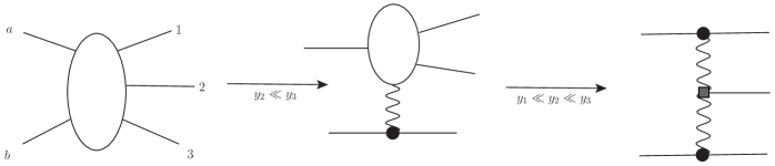
Figure 10: The factorisation property still applies whenever there is a strong rapidity order imposed, even if not the full MRK limit.

If the only requirement on the ordered rapidities is a large difference between $y_{n-1}$ and $y_{n}$ ($y_{n-1}\ll y_{n}$, i.e. $\forall\{i,j,k,l\}\in\{1,\ldots,n-1\},i\not=j,k\not=l:s_{ij}\sim s_{kl},s_{in}\sim s_{jn}$), but no further requirement on a large difference between any of $y_{1},y_{2},...,y_{n}$, then the leading power of the amplitude can still be written as a contraction of the quark current with a sub-amplitude, depending only on the reduced set of momenta $p_{a},p_{1},\ldots,p_{n-1}$:

$$\mathcal{M}\sim\mathcal{M}_{\text{sub}}^{\mu}(p_{a},p_{1},...,p_{n-1})\frac{1}{t_{n-1}}j_{\mu}(p_{b},p_{n})$$ (36)

In the stricter MRK limit of large rapidity differences between all $1,\ldots,n-1$, the sub-amplitude $\mathcal{M}_{\text{sub}}^{\mu}(p_{a},p_{1},...,p_{n-1})$ would factorise further into another quark current, Lipatov vertices, and $t$-channel propagators, as indicated on the right-hand side of Fig. 10. Clearly, the more complicated sub-amplitude $\mathcal{M}_{\text{sub}}^{\mu}(p_{a},p_{1},...,p_{n-1})$ includes the leading-power behaviour in the full MRK limit, and hence one can recover this fully factorised form starting from Eq. (36).

In order to extend the current-based formalism of HEJ to include the first next-to-leading logarithmic corrections, we will therefore need to extract a form $j_{\mu}^{\rm uno}(p_{1},p_{g},p_{a})$, which takes the place of $\mathcal{M}_{\text{sub}}^{\mu}(p_{a},p_{1},...,p_{n-1})$ in Eq. (36). Here, we have (without loss of generality) considered the case of $y_{1}\sim y_{g}\ll y_{2}$. We then seek an expression for a quantity $j_{\mu}^{\rm uno}(p_{1},p_{g},p_{a})$ such that the equation

$$\mathcal{M}_{{\rm tree}\ qQ\to gqQ}^{\rm HEJ}=-g_{s}^{3}T^{d}_{2b}\ \frac{j^{{\rm uno}\ cd}_{\mu}(p_{1},p_{g},p_{a})j^{\mu}(p_{2},p_{b})}{t_{b2}}$$ (37)

will contain all the leading-power behaviour of the full tree-level amplitude. We will give the new current a superscript uno, since it will be used only for the calculation of unordered emissions, $y_{g}<y_{1}$. Emissions in-between the quarks, $y_{1}<y_{g}$, are already accounted for using the real and virtual corrections described in the previous section and so we do not apply this correction there. The new current now carries colour indices $cd$, where $c$ is the colour of the emitted gluon, and $d$ is the colour of the gluon exchanged in the $t$-channel.

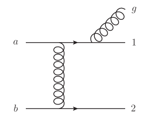
Figure 11: One of the diagrams which contribute to the process $qQ\to gqQ$, illustrating the labelling convention used throughout this section. We will consider the case where $y_{g}\sim y_{1}\ll y_{2}$. $a$ ($b$) is the incoming quark in the backward (forward) direction respectively, which we here assume to be of different flavours.

One of the five Feynman diagrams which contribute to this process is shown in Fig. 11, which also defines the momentum labelling. The exact tree-level expression for the sum of all five diagrams is:

$$\begin{split}\mathcal{M}_{\rm tree}=&(ig_{s})^{3}\ T^{c}_{1i}T^{d}_{ia}T^{d}_{2b}\ \varepsilon_{g\nu}\frac{\langle 1|\nu|g\rangle\langle g|\mu|a\rangle+2p_{1}^{\nu}\langle 1|\mu|a\rangle}{s_{1g}t_{b2}}\langle 2|\mu|b\rangle\\ +&(ig_{s})^{3}\ T^{d}_{1i}T^{c}_{ia}T^{d}_{2b}\ \varepsilon_{g\nu}\frac{2p_{a}^{\nu}\langle 1|\mu|a\rangle-\langle 1|\mu|g\rangle\langle g|\nu|a\rangle}{t_{ag}t_{b2}}\langle 2|\mu|b\rangle\\ +&(ig_{s})^{3}\ T^{c}_{2i}T^{d}_{ib}T^{d}_{1a}\ \varepsilon_{g\nu}\frac{\langle 2|\nu|g\rangle\langle g|\mu|b\rangle+2p_{2}^{\nu}\langle 2|\mu|b\rangle}{s_{2g}t_{a1}}\langle 1|\mu|a\rangle\\ +&(ig_{s})^{3}\ T^{d}_{2i}T^{c}_{ib}T^{d}_{1a}\ \varepsilon_{g\nu}\frac{2p_{b}^{\nu}\langle 2|\mu|b\rangle-\langle 2|\mu|g\rangle\langle g|\nu|b\rangle}{t_{bg}t_{a1}}\langle 1|\mu|a\rangle\\ -&g_{s}^{3}\ f^{dec}T^{d}_{1a}T^{e}_{2b}\ \varepsilon_{g\nu}\frac{\langle 1|\rho|a\rangle\langle 2|\mu|b\rangle}{t_{a1}t_{b2}}\left(2p_{g}^{\mu}g^{\nu\rho}-2p_{g}^{\rho}g^{\mu\nu}-(q_{1}+q_{2})^{\nu}g^{\mu\rho}\right),\end{split}$$ (38)

where we have used the shorthands

$$\langle i|\mu|j\rangle=\bar{u}^{-}(p_{i})\gamma^{\mu}u^{-}(p_{j}),\qquad s_{ij}=(p_{i}+p_{j})^{2},\qquad t_{ij}=(p_{i}-p_{j})^{2},$$ (39)

and the $T^{c}_{ij}$ are colour matrices. The external gluon carries the colour index $c$, and $\{a,b,1,2\}$ in the subscript indicates the colour index of the relevant external quark. Repeated indices are summed over. Of course, this expression can be considerably simplifed by contracting the Lorentz indices and re-arranging. However, we choose not to do so here as the extended form is particularly convenient for the discussion below.

In the MRK limit, where $y_{1}\ll y_{g}\ll y_{2}$, one term in each of the first four lines of Eq. (38) becomes sub-dominant (the term with numerator dependence on $p_{g}$). This is most easily seen by performing the Lorentz contractions. In this case, the expression becomes [30]

$$\begin{split}\mathcal{M}_{\rm tree}^{FKL}&=-g_{s}^{3}f^{dec}T^{d}_{1a}T^{e}_{2b}\ \varepsilon_{g\nu}\ \frac{\langle 1|\mu|a\rangle\langle 2|\mu|b\rangle}{t_{a1}t_{b2}}\ V_{L}^{\nu}\\ &=-g_{s}^{3}f^{dec}T^{d}_{1a}T^{e}_{2b}\ \varepsilon_{g\nu}\ \frac{j^{\mu}(p_{1},p_{a})j_{\mu}(p_{2},p_{b})}{t_{a1}t_{b2}}\ V_{L}^{\nu},\end{split}$$ (40)

analogously to Eq. (20), and illustrated by the right-hand diagram of Fig. 10. However, for the case at hand, we no longer want to assume a strong ordering between $y_{g}$ and $y_{1}$. In this case, the only sub-dominant terms are the $p_{g}$-dependent terms in the numerator in lines 3 and 4 of Eq. (38). We observe that by discarding these two terms, every other term immediately appears in the form $j^{\mu}(p_{2},p_{b})\times X_{\mu}$. The sum of these $X_{\mu}$-pieces will therefore become our unordered current.

We now turn our attention to colour factors. The ‘$b$-$2$’ end of the chain has to have a single colour matrix of the form $T^{d}_{2b}$, for a dummy index $d$, in order to be consistent with the factorised picture; this is to ensure it can be contracted with either a normal quark- or gluon-current, or the unordered two-particle $j_{\mu}^{\rm uno}(p_{1},p_{g},p_{a})$. This is already the case for the first, second and fifth lines of Eq. (38). The MRK limit implies $p_{b}\simeq p_{2}=p_{+}$ and the dominant terms in the 3rd and 4th lines are:

$$\begin{split}&-ig_{s}^{3}\ \langle 1|\mu|a\rangle\langle 2|\mu|b\rangle\ \varepsilon_{g\nu}\left(\frac{2p_{2}^{\nu}}{t_{a1}s_{2g}}T^{c}_{2i}T^{d}_{ib}T^{d}_{1a}+\frac{2p_{b}^{\nu}}{t_{bg}t_{a1}}T^{d}_{2i}T^{c}_{ib}T^{d}_{1a}\right)\\ \simeq&-ig_{s}^{3}\ \langle 1|\mu|a\rangle\langle 2|\mu|b\rangle\ \varepsilon_{1\nu}\ \frac{1}{t_{a1}}\frac{p_{+}^{\nu}}{p_{+}\cdot p_{g}}\ T^{d}_{1a}\left(T^{c}_{2i}T^{d}_{ib}-T^{d}_{2i}T^{c}_{ib}\right)\\ =&\quad\;\,g_{s}^{3}\ \langle 1|\mu|a\rangle\langle 2|\mu|b\rangle\ \varepsilon_{1\nu}\ \frac{1}{t_{a1}}\frac{p_{+}^{\nu}}{p_{+}\cdot p_{g}}\ f^{cde}T^{d}_{1a}T^{e}_{2b}\\ \simeq&\ g_{s}^{3}\ \langle 1|\mu|a\rangle\langle 2|\mu|b\rangle\ \varepsilon_{g\nu}\ \ f^{cde}T^{d}_{1a}T^{e}_{2b}\ \ \frac{1}{2t_{a1}}\left(\frac{p_{b}^{\nu}}{(p_{b}\cdot p_{g})}+\frac{p_{2}^{\nu}}{(p_{2}\cdot p_{g})}\right).\end{split}$$ (41)

We have chosen to restore the symmetry of $p_{b}$ and $p_{2}$ in the last line (as we do in $V_{L}^{\nu}$ above). The MRK limit is of course independent of such choices. We then arrive at the following expression for the amplitude for quark-quark scattering with an additional unordered gluon emission:

$$\mathcal{M}_{{\rm tree}\ qQ\to gqQ}^{HEJ}=-g_{s}^{3}\frac{\langle 2|\mu|b\rangle\varepsilon_{1\nu}}{t_{b2}}T_{2b}^{d}\left(iT_{1i}^{c}T_{ia}^{d}\ U_{1}^{\mu\nu}+iT_{1i}^{d}T_{ia}^{c}\ U_{2}^{\mu\nu}+f^{ecd}T_{1a}^{e}\ L^{\mu\nu}\right).$$ (42)

The tensors $U_{1}^{\mu\nu}$, $U_{2}^{\mu\nu}$ and $L^{\mu\nu}$ may then be read off from Eqs. (38) and (41) as

$$\begin{split}U_{1}^{\mu\nu}&=\frac{1}{s_{1g}}\left(j_{1g}^{\nu}j_{ga}^{\mu}+2p_{1}^{\nu}j_{1a}^{\mu}\right)\qquad\qquad U_{2}^{\mu\nu}=\frac{1}{t_{ag}}\left(2j_{1a}^{\mu}p_{a}^{\nu}-j_{1g}^{\mu}j_{ga}^{\nu}\right)\\ L^{\mu\nu}&=\frac{1}{t_{a1}}\left(-2p_{g}^{\mu}j_{1a}^{\nu}+2p_{g}.j_{1a}g^{\mu\nu}+(q_{1}+q_{2})^{\nu}j_{1a}^{\mu}+\frac{t_{b2}}{2}j_{1a}^{\mu}\left(\frac{p_{2}^{\nu}}{p_{g}.p_{2}}+\frac{p_{b}^{\nu}}{p_{g}.p_{b}}\right)\right).\end{split}$$ (43)

The three colour factors in Eq. (42) are not independent and can be combined to give

$$\mathcal{A}_{qQ\to gqQ}=-ig_{s}^{3}\ \frac{\langle 2|\mu|b\rangle\varepsilon_{g\nu}}{t_{b2}}\ T_{2b}^{d}\left(T_{1i}^{c}T_{ia}^{d}\ \left(U_{1}^{\mu\nu}-L^{\mu\nu}\right)+T_{1i}^{d}T_{ia}^{c}\ \left(U_{2}^{\mu\nu}+L^{\mu\nu}\right)\right).$$ (44)

By comparison to Eq. (37), we extract

$$j^{{\rm uno}\;\mu\ cd}(p_{1},p_{g},p_{a})=i\varepsilon_{g\nu}\left(T_{1i}^{c}T_{ia}^{d}\ \left(U_{1}^{\mu\nu}-L^{\mu\nu}\right)+T_{1i}^{d}T_{ia}^{c}\ \left(U_{2}^{\mu\nu}+L^{\mu\nu}\right)\right).$$ (45)

Gauge-invariance of this new current is satisfied throughout phase space; it is easily checked that replacing $\varepsilon_{g\nu}$ with $p_{g\nu}$ gives identically zero. One can also check that the use of Eq. (45) in the MRK limit will result in the BFKL NLO impact factor derived in Ref.[49].

After some colour algebra, the final summed and averaged amplitude for $q(p_{a})\ Q(p_{b})\to g(p_{g})\ q(p_{1})\ Q(p_{2})$ is then given by

$$\begin{split}\left|\overline{\mathcal{M}_{{\rm tree}\ qQ\to gqQ}^{HEJ}}\right|^{2}=&-\frac{g_{s}^{6}}{16t_{b2}^{2}}\ \sum_{h_{a},h_{1},h_{b},h_{2}}\ \bigg{[}C_{F}\big{(}2\mathrm{Re}\big{(}[(L^{\mu\nu}-U_{1}^{\mu\nu})\cdot j_{2b\,\mu}]\ [(L^{\rho}_{\;\,\nu}+U_{2\;\,\nu}^{\;\rho})\cdot j_{2b\,\rho}]^{*}\big{)}\big{)}\\ &\hskip 113.81102pt+2\frac{C_{F}^{2}}{C_{A}}\left|(U_{1}^{\mu\nu}+U_{2}^{\mu\nu})\cdot j_{2b_{\mu}}\right|^{2}\bigg{]}\\ \equiv&-\frac{g_{s}^{6}}{16t_{b2}^{2}}C_{F}\left\|S_{f_{1}f_{2}\to gf_{1}f_{2}}^{\rm uno}\right\|^{2},\end{split}$$ (46)

where the sum runs over the helicities of the four quarks and the square in the second line indicates contraction over the $\nu$-index. The final line defines the function $S^{\rm uno}$ and is analogous to the rapidity-ordered case described in Eq. (21).

We now follow the formalism for additional ordered emissions derived in section 2.3 to arrive at the following HEJ matrix element in $4-2\epsilon$ dimensions for $f_{1}f_{2}\to gf_{1}\cdot g\cdot f_{2}$, where $f_{1}$ now must be a quark (cf. Eq. (26):

$$\begin{split}\overline{\left|\mathcal{M}^{\rm HEJ}_{\varepsilon\ qf_{2}\to gq\cdot g\cdot f_{2}}\right|}^{2}=\ &\frac{1}{4\ (N_{\!C}^{2}-1)}\ g_{s}^{2}\ \left\|S^{\rm uno}_{qf_{2}\to gqf_{2}}\right\|^{2}\\ &\cdot\ \left(g_{s}^{2}\ C_{F}\ \frac{1}{t_{1}}\right)\cdot\ \left(g_{s}^{2}\ K_{f_{2}}\ \frac{1}{t_{n-1}}\right)\\ &\cdot\prod_{i=1}^{n-2}\left(\frac{-g_{s}^{2}C_{A}}{t_{i}t_{i+1}}\ V^{\mu}(q_{i},q_{i+1})V_{\mu}(q_{i},q_{i+1})\right)\\ &\cdot\prod_{j=1}^{n-1}\exp\left[2\hat{\alpha}(q_{j})(y_{j+1}-y_{j})\right].\end{split}$$ (47)

We are now ready to build the regularised matrix-element with the appropriate all-order corrections in the manner of Section 2.4. Such corrections can be added for gluon emissions in the phase space delimited by the rapidity(ies) of the final state quark(s). This region will be denoted the all-order summation region. The momenta of the quarks are still required to be hard, and form part of the two jets extremal (but one) in rapidity. One current includes the unordered gluon emission, which allows for a single gluon to be emitted outside this all-order summation region. Such an unordered gluon is required to enter a separate hard jet from that of the quark, since the associated collinear singularity is otherwise unregulated: it would cancel with the singularity associated with the one-loop correction to the quark production, which form part of the full NLL corrections, which are not yet included in the formalism. However, in the all-order summation region, the infrared singularities cancel as discussed in the previous section. We therefore find

$$\begin{split}\overline{\left|\mathcal{M}^{\rm HEJ}_{qf_{2}\to gq\cdot g\cdot f_{2}}\right|}^{2}=\ &\frac{1}{4\ (N_{\!C}^{2}-1)}\ g_{s}^{2}\ \left\|S_{qf_{2}\to gqf_{2}}^{\rm uno}\right\|^{2}\\ &\cdot\ \left(g_{s}^{2}C_{F}\ \frac{1}{t_{1}}\right)\cdot\ \left(g_{s}^{2}\ K_{f_{2}}\ \frac{1}{t_{n-1}}\right)\\ &\cdot\prod_{i=1}^{n-2}\left(\frac{-g_{s}^{2}C_{A}}{t_{i}t_{i+1}}\ V^{\mu}(q_{i},q_{i+1})V_{\mu}(q_{i},q_{i+1})\right)\\ &\cdot\prod_{j=1}^{n-1}\exp\left[\omega^{0}(q_{j\perp})(y_{j+1}-y_{j})\right].\end{split}$$ (48)

There is a corresponding equation for the gluon emitted instead forward of the most forward quark, $f_{2}$.

The currents for the unordered emission therefore enter the calculation of the all-order, leading corrections to the Born-level three-jet processes with a gluon jet of larger absolute rapidity than that of the respective quark jet. These three-jet events form part of the sub-leading logarithmic corrections to inclusive dijet production.

2.6 High Energy Corrections to Higgs Boson Production with Jets

In order to develop the formalism for unordered emissions, we have so far worked with amplitudes purely within QCD. However, it is straight-forward to extend the HEJ description of jet processes to include the production also of a Higgs boson. In this paper in particular we are concerned with the production of a Higgs boson with at least two jets so in this section we briefly review the existing HEJ description of this process first developed in [30]. This makes use of the infinite top-mass limit, but this limit not only commutes with the high-energy limit[50], but results can be obtained for the high-energy limit without applying the infinite top-mass limit. We leave such investigations for a future study, but will here add the possibility of unordered gluon emissions derived in the previous subsection to the amplitudes derived in Ref. [30] for Higgs boson production in association with jets. This will result in different formulae for the high-energy approximations to the scattering amplitude for the various rapidity-orderings of particles. We discuss each here in turn.

2.6.1 Higgs Boson with Rapidity Between that of Hard Jets

We begin with the HEJ approximation to the tree-level amplitude for $qQ\to HqQ+(n-2)g$. From the discussion in the previous section, the dominant momentum configurations in the MRK limit are those where the gluons are all emitted between the two quarks in rapidity. We will exploit the factorisation of the amplitudes discussed in the previous subsection (and which still holds when a Higgs boson is included) to describe an amplitude as the contraction of two currents over a $ggH$-vertex, multiplied by a product of vertices for each additional gluon emission. This is illustrated schematically in Fig. 12 for the case where the Higgs boson is also between the outer quark jets in rapidity, between gluons $j$ and $j+1$.

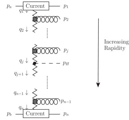
Figure 12: The analytic structure of the base tree-level scattering amplitude for $qQ\to HqQ+(n-2)g$ in High Energy Jets. In this case, the Higgs boson is emitted between gluons $j$ and $j+1$ in rapidity.

This figure also gives the definitions of the momenta $p_{i}$ and $q_{j}$ used in this section. The vertices for additional gluon emissions depend on the momenta of that emission and the momenta of the parton of maximum and minimum rapidity, but not on the momenta of any other emissions or the Higgs boson. The amplitude can then be written [51, 52, 30]

$$\begin{split}\mathcal{M}^{\rm HEJ}_{\rm tree\ qQ\to Hq\cdot g\cdot Q}&=-g_{s}^{2}T^{a_{1}}_{i_{1}i_{a}}T^{a_{n-1}}_{i_{n}i_{b}}\ \frac{\mathcal{S}_{qQ\to qQH}(p_{1},p_{n},p_{a},p_{b},q_{j},q_{j+1})}{\sqrt{q_{1}^{2}q_{j}^{2}q_{j+1}^{2}q_{n}^{2}}}\\ &\hskip 28.45274pt\times\prod_{k=2}^{j}ig_{s}f^{a_{k-1}b_{k}a_{k}}\ \frac{\varepsilon_{\nu_{k}}(p_{k})V^{\nu_{k}}_{L}(q_{k-1},q_{k})}{\sqrt{q_{k-1}^{2}q_{k}^{2}}}\\ &\hskip 28.45274pt\times\prod_{k=j+1}^{n-1}ig_{s}f^{a_{k-1}b_{k}a_{k}}\ \frac{\varepsilon_{\nu_{k}}(p_{k})V^{\nu_{k}}_{L}(q_{k},q_{k+1})}{\sqrt{q_{k}^{2}q_{k+1}^{2}}}.\end{split}$$ (49)

Here $i_{j}$ and $b_{k}$ are the colour indices of the relevant quark and the $k$th external gluon and the $a_{j}$ indices are summed over. The expression $\mathcal{S}_{qQ\to qQH}(p_{1},p_{n},p_{a},p_{b},q_{j},q_{j+1})$ represents the contraction of the two end currents with the $ggH$-vertex in the limit of infinite top mass:

$$\begin{split}&\mathcal{S}_{qQ\to qQH}(p_{1},p_{n},p_{a},p_{b},q_{j},q_{j+1})=j_{\mu}(p_{1},p_{a})j_{\nu}(p_{n},p_{b})V_{H}^{\mu,\nu}(q_{j},q_{j+1}),\\ {\rm where}\ V_{H}^{\mu,\nu}&(q_{j},q_{j+1})=\left(\frac{\alpha_{s}}{3\pi v}\right)\left(g^{\mu\nu}q_{j}.q_{j+1}-q_{j}^{\nu}q_{j+1}^{\mu}\right),\qquad j_{\mu}(p_{o},p_{i})=\bar{u}(p_{o})\gamma_{\mu}u(p_{i}).\end{split}$$ (50)

The two products which represent the gluon emissions are separated at the point where the Higgs boson occurs in rapidity in order to correctly assign the relevant $q_{i}$. Our description of processes with incoming gluons follows the same prescription as that for pure QCD processes. The relevant quark current(s) in Eq. (50) have the same form multiplied by a scalar factor.

We now wish to include the emission of an unordered gluon in the description of these Higgs boson processes. In section 2.5, the only modification to the ordered process was in the spinor factor. Comparing Eq. (34) and (48),

$$\left\|S_{f_{1}f_{2}\to f_{1}f_{2}}\right\|^{2}\ \rightarrow\ \left\|S_{qf_{2}\to gqf_{2}}^{\rm uno}\right\|^{2}.$$ (51)

The factorisation property of the amplitudes implies that we may apply the same prescription here. The infrared divergences are regulated here in the same way as in the pure QCD amplitudes. The virtual corrections are still given by the Lipatov ansatz with the prescription given in Eq. (24), which leads to the following infrared finite amplitude for a Higgs boson produced between particles $j$ and $j+1$ in rapidity (c.f. Eq. (34)):

$$\begin{split}\overline{\left|\mathcal{M}^{\rm HEJ}_{\ f_{1}f_{2}\to Hgf_{1}\cdot g\cdot f_{2}}\right|}^{2}=&\frac{1}{4(N_{C}^{2}-1)}\left\|\mathcal{S}_{qQ\to qQH}^{\rm uno}(p_{1},p_{g},p_{n},p_{a},p_{b},q_{j},q_{j+1})\right\|^{2}\\ &\cdot\left(g_{s}^{2}K_{f_{1}}\frac{1}{t_{1}}\right)\cdot\left(g_{s}^{2}K_{f_{2}}\frac{1}{t_{n}}\right)\\ &\cdot\prod_{k=2}^{j}\left(\frac{-g_{s}^{2}C_{A}}{t_{k_{1}}t_{k}}V^{\nu_{k}}(q_{k-1},q_{k})V_{\nu_{k}}(q_{k-1},q_{k})\right)\\ &\cdot\prod_{k=j+1}^{n-1}\left(\frac{-g_{s}^{2}C_{A}}{t_{k}t_{k+1}}V^{\nu_{k}}(q_{k},q_{k+1})V^{\nu_{k}}(q_{k},q_{k+1})\right)\\ &\cdot\prod_{i=1}^{j-1}\exp\left[\omega^{0}(q_{i\perp})(y_{i+1}-y_{i})\right]\cdot\prod_{i=j+2}^{n}\exp\left[\omega^{0}(q_{i\perp})(y_{i}-y_{i-1})\right]\\ &\cdot\exp\left[\omega^{0}(q_{j\perp})(y_{H}-y_{j})\right]\cdot\exp\left[\omega^{0}(q_{j+1\perp})(y_{j+1}-y_{H})\right],\end{split}$$ (52)

where now

$$\mathcal{S}_{qQH}^{\rm uno}(p_{1},p_{g},p_{n},p_{a},p_{b},q_{i},q_{i+1})=j^{{\rm uno}}_{\mu}(p_{1},p_{g},p_{a})j_{\nu}(p_{n},p_{b})V_{\mu\nu}^{H}(q_{i-1},q_{i}),$$ (53)

for a gluon emission most backward in rapidity of all coloured particles. The modified current $j^{\rm uno}_{\mu}(p_{1},p_{g},p_{a})$ is exactly the one given in Eq. (45). If, instead, the unordered emission is forward in rapidity of all coloured particles, the current pair $j_{\mu}(p_{1},p_{g},p_{a})j_{\nu}(p_{n},p_{b})$ becomes $j_{\mu}(p_{1},p_{a})j_{\nu}^{\rm uno}(p_{n},p_{g},p_{b})$.

2.6.2 Higgs Boson with Rapidity Outside that of Hard Jets

The remaining case to consider is the case where the Higgs boson is produced outside of the coloured particles in rapidity, see e.g. Fig. 13(b). Motivated by the amplitude for $qQ\to qQH$ (where of course there is just one $t$-channel amplitude applied for all momentum configurations), we will apply the leading factorised amplitude, which is the configuration where the Higgs-boson vertex is the first (last) vertex in the $t$-channel chain if the rapidity of the Higgs boson is less (greater) than the rapidity of the quarks. Therefore, in practice, the two configurations in Figs. 13(a) and (b) have the same description. When the Higgs boson is produced outside of the coloured particles in rapidity, we will only include unordered gluon emissions where these occur at the opposite end of the chain to the Higgs boson (all possibilities could in principle be included, but these are perturbative corrections to already suppressed configurations). The matrix element squared in this case is then given by Eq. (52) with $j=1$ if the Higgs is most backward in rapidity. It has $j=n-1$ if the Higgs is most forward in rapidity and $j_{\mu}(p_{1},p_{a})j_{\nu}^{\rm uno}(p_{n},p_{g},p_{b})$ in place of $j^{\rm uno}_{\mu}(p_{1},p_{g},p_{a})j_{\nu}(p_{n},p_{b})$ in Eq. (53). For example, the all-order equation corresponding to an unordered gluon emission as the most backward outgoing particle and a Higgs boson as the most forward outgoing particle (the $n$-emission equivalent of Fig. 13(b)) is given by:

$$\begin{split}\overline{\left|\mathcal{M}^{\rm HEJ}_{\ f_{1}f_{2}\to gf_{1}\cdot g\cdot f_{2}H}\right|}^{2}=&\frac{1}{4(N_{C}^{2}-1)}\left\|\mathcal{S}_{qQ\to qQH}^{\rm uno}(p_{1},p_{g},p_{n},p_{a},p_{b},q_{n-1},q_{n})\right\|^{2}\\ &\cdot\left(g_{s}^{2}K_{f_{1}}\frac{1}{t_{1}}\right)\cdot\left(g_{s}^{2}K_{f_{2}}\frac{1}{t_{n}}\right)\\ &\cdot\prod_{k=2}^{n-1}\left(\frac{-g_{s}^{2}C_{A}}{t_{k_{1}}t_{k}}V^{\nu_{k}}(q_{k-1},q_{k})V_{\nu_{k}}(q_{k-1},q_{k})\right)\\ &\cdot\prod_{i=1}^{n-2}\exp\left[\omega^{0}(q_{i\perp})(y_{i+1}-y_{i})\right]\\ &\cdot\exp\left[\omega^{0}(q_{n-1\perp})(y_{H}-y_{n-1})\right]\cdot\exp\left[\omega^{0}(q_{n\perp})(y_{n}-y_{H})\right],\end{split}$$ (54)

where $q_{n}=q_{n-1}-p_{H}$ in clear analogy to Eq. (52) with $j=n-1$.

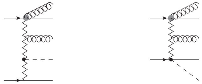
(a)                                                              (b) a

Figure 13: Sample diagrams for a Higgs+3j process including an unordered gluon emission: (a) the Higgs is emitted in between the jet system in rapidity and (b) the Higgs is emitted outside via an adapted current.

If the flavour $f_{1}$ (or $f_{2}$) is a gluon, the amplitude for the emission of a Higgs boson with more extremal rapidity than the gluons receives contributions also from top box diagrams, not just the triangle diagrams implemented in the formalism of the currents. We will use the amplitude derived for the strict MRK limit in Ref. [50] for these kinematic configurations. Their contribution is suppressed for large rapidity spans, but they are included for completeness.

2.6.3 Perturbative Validation of the Approximations

We now test the quality of the approximation by comparing this result with the full matrix element result taken from Madgraph [40] order-by-order in the strong coupling. In Fig. 14, we compare the matrix element squared for $ud\to guHd$ in a slice through phase space where the rapidities are chosen to be: $y_{g}=-\Delta$, $y_{u}=-\Delta/3$, $y_{H}=\Delta/3$ and $y_{d}=\Delta$ for $\Delta\in\{0,10\}$. The matrix-element squared has been multiplied by one power of the $gu$ invariant mass, $s_{12}$, to counteract the suppression discussed in Section 2.1.1. We observe very close agreement throughout the rapidity range between the full MadGraph result (red, solid) and the unordered HEJ formalism (green, dashed).

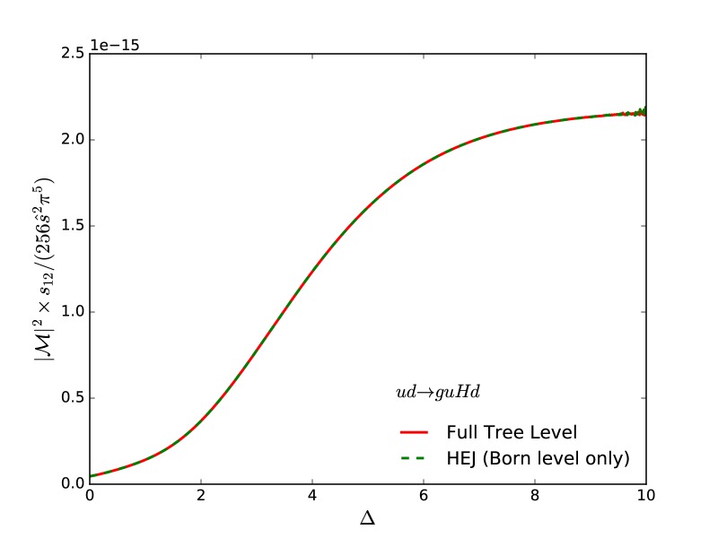
Figure 14: A slice through phase space of $\left|\overline{\cal M}\right|^{2}\times s_{12}/(256\pi^{5}\hat{s}^{2})$ for the process $ud\to guHd$. The rapidities of the final-state particles are chosen to be $y_{g}=-\Delta$, $y_{u}=-\Delta/3$, $y_{H}=\Delta/3$ and $y_{d}=\Delta$. The new HEJ description of this unordered configuraton (“HEJ (Born level only)”, green dashed) shows close agreement to the full tree level result (red solid) throughout the range.

In Fig. 15 we show the distribution of the rapidity difference between the most forward and backward hard jet again for the process $ud\to guHd$, integrated over the region of phase space where $y_{g}<y_{u}<y_{H}<y_{Q}$. We apply modest jet cuts, requiring the partons to form 3 jets with $p_{T}>30$ GeV and $|y|<4.4$. Here, we consider on-shell Higgs-boson production and require $|y_{H}|<2.37$. It is clear that the description from the new impact factor describing unordered emissions tracks the result from the full matrix element extremely closely throughout the full range of $\Delta y_{fb}$, becoming indistinguishable at large $\Delta y_{fb}$.

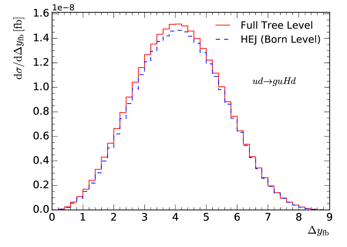
Figure 15: The rapidity span distribution for $ud\to guHd$ events after integration over phase space in the region where the gluon is the most backward final state particle: $y_{g}<y_{u}<y_{H}<y_{d}$ and $\Delta y_{fb}=y_{d}-y_{g}$. The approximation (“HEJ Born level”, blue dashed) gives an extremely good description of the full tree-level matrix element (red, solid).

The square of the matrix elements can be trivially extended to include, for example, the diphoton decay of the Higgs boson by simply multiplying the square of the matrix elements of either the FKL-ordered (Eq. (34)) or unordered configuration (Eq. (52)) by the branching ratio, $BR(H\to\gamma\gamma)$, and generating the decay products isotropically. This is available as an option in the code.

2.7 Matching and Merging of Fixed Order Samples and Final Results

Using the formalism outlined in the previous sections, the all-order summed contribution to the FKL-ordered plus first unordered cross section for the production of a Higgs boson which decays to two photons in association with at least two jets can now be found as

$$\begin{split}\sigma_{H+2j}^{\mathrm{resum}}=&\sum_{f_{a},f_{b}}\ \sum_{n=2}^{\infty}\ \left(\int_{p_{1\perp}=p_{\perp\mathrm{ext,min}}}^{\infty}\frac{\mathrm{d}^{2}\mathbf{p}_{1\perp}}{(2\pi)^{3}}\ \int_{y_{\mathrm{min}}}^{y_{\mathrm{max}}}\frac{\mathrm{d}y_{1}}{2}\right)\ \left(\int_{p_{n\perp}=p_{\perp\mathrm{ext,min}}}^{\infty}\frac{\mathrm{d}^{2}\mathbf{p}_{n\perp}}{(2\pi)^{3}}\ \int_{y_{n-1}}^{y_{\mathrm{max}}}\frac{\mathrm{d}y_{n}}{2}\right)\\ &\times\prod_{i=2}^{n-1}\left(\int_{p_{i\perp}=\kappa}^{\infty}\frac{\mathrm{d}^{2}\mathbf{p}_{i\perp}}{(2\pi)^{3}}\ \int_{y_{i-1}}^{y_{\mathrm{max}}}\frac{\mathrm{d}y_{i}}{2}\right)\ \int\frac{\mathrm{d}^{3}p_{\gamma_{1}}}{(2\pi)^{3}\ 2E_{\gamma_{1}}}\ \ \int\frac{\mathrm{d}^{3}p_{\gamma_{2}}}{(2\pi)^{3}\ 2E_{\gamma_{2}}}\ \\ &\times\frac{\overline{|\mathcal{M}_{\mathrm{HEJ}}^{\mathrm{reg}}(\{p_{i},p_{\gamma_{1}},p_{\gamma_{2}}\},\mu_{R},\lambda)|}^{2}}{\hat{s}^{2}}\cdot\ x_{a}f_{f_{a}}(x_{a},Q_{a})\ \cdot x_{b}f_{f_{b}}(x_{b},Q_{b})\\ &\times(2\pi)^{4}\ \delta^{2}\!\!\left(\sum_{k=1}^{n}\mathbf{p}_{k\perp}+p_{\gamma_{1}\perp}+p_{\gamma_{2}\perp}\right)\ \mathcal{O}_{2j}(\{p_{i}\}),\end{split}$$ (55)

where in principle $y_{\mathrm{min}}=-\infty$ and $y_{\mathrm{max}}=\infty$ (in practice, they can both technically be put to $\pm 5$ because of the requirement that the extremal partons form part of the observed extremal jets). Furthermore, we will choose by default $\kappa=0.2$ GeV and $\lambda=\kappa$ (see Section 2.4 for the definition of these regulators). $\kappa$ has to be chosen small (as close to 0 as possible), and setting $\lambda=\kappa$ ensures that events are generated with positive weight only. While the correct results are obtained in the limit $\lambda\to 0$, the results are stable below $\lambda=2$ GeV. The factors of $x_{i}f_{i,f_{i}}(x_{i},Q_{i})$, $i=a,b$, are the parton density functions for a parton of flavour $f_{i}$ evaluated at momentum fraction $x_{i}$ and factorisation scale $Q_{i}$. In practice, we take both $Q_{a}$ and $Q_{b}$ to be equal to the factorisation scale $\mu_{F}$ which can be taken to be either fixed or a number of dynamic scales (including $H_{T}/2$ or the maximum $p_{T}$ of any single jet). The renormalisation scale $\mu_{R}$ may also be evaluated at a fixed or dynamic scale. The step function, $\mathcal{O}_{2j}(\{p_{i}\})$, implements the chosen cuts of the process, which consists of a minimum requirement that at least two hard jets are observed.

The expression in Eq. (55) has leading-logarithmic accuracy by construction. We can impose leading-order fixed-order accuracy through matching to leading-order matrix elements. Eq. (55) only describes FKL momentum configurations or FKL momentum configurations with one extra unordered emission, hereafter referred to together as “HEJ configurations”. We therefore implement matching to full fixed-order in two different ways, depending on the flavour and momentum configuration.

Firstly, for the HEJ configurations covered by the formula above (i.e. those where higher-order corrections are systematically summed), we employ multiplicative matching to leading-order accuracy, where the final state partons generated by the all-order results is clustered into two or three jets. These jets can be formed from a higher number of partons, which means that they are not necessarily on-shell. Since the evaluation of leading-order matrix elements require particles with on-shell momenta, we reshuffle the jet-momenta to put them on-shell, using an algorithm described in [32]. After this the matching is implemented by multiplying the HEJ matrix-element-squared by the factor

$$w_{H+n\rm{-jet}}\equiv\frac{\overline{\left|\mathcal{M}^{LO}_{f_{1}f_{2}\to f_{1}\cdot g\cdot f_{2}H}\left(\left\{j_{i}\right\}\right)\right|}^{2}}{\overline{\left|\mathcal{M}^{HEJ}_{{\rm tree}\ f_{1}f_{2}\to f_{1}\cdot g\cdot f_{2}H}\left(\left\{j_{i}\right\}\right)\right|}^{2}},$$ (56)

where $\{j_{i}\}$ are the on-shell jet-momenta.

An alternative way to think of this procedure is to view the matching as a merging procedure as used routinely for parton showers (CKKW-L[36, 37]) for leading-order matrix elements at different orders where in place of the logarithms controlled by a parton shower prescription, the logarithms instead are those which are leading in the high-energy limit. This procedure gives

$$\begin{split}\sigma_{H+2j}^{\mathrm{resum,\ match}}=&\sum_{f_{a},f_{b}}\ \sum_{n=2}^{\infty}\ \left(\int_{p_{1\perp}=p_{\perp\mathrm{ext,min}}}^{\infty}\frac{\mathrm{d}^{2}\mathbf{p}_{1\perp}}{(2\pi)^{3}}\ \int_{y_{\mathrm{min}}}^{y_{\mathrm{max}}}\frac{\mathrm{d}y_{1}}{2}\right)\ \left(\int_{p_{n\perp}=p_{\perp\mathrm{ext,min}}}^{\infty}\frac{\mathrm{d}^{2}\mathbf{p}_{n\perp}}{(2\pi)^{3}}\ \int_{y_{n-1}}^{y_{\mathrm{max}}}\frac{\mathrm{d}y_{n}}{2}\right)\\ &\prod_{i=2}^{n-1}\left(\int_{p_{i\perp}=\kappa}^{\infty}\frac{\mathrm{d}^{2}\mathbf{p}_{i\perp}}{(2\pi)^{3}}\ \int_{y_{i-1}}^{y_{\mathrm{max}}}\frac{\mathrm{d}y_{i}}{2}\right)\ \int\frac{\mathrm{d}^{3}p_{\gamma_{1}}}{(2\pi)^{3}\ 2E_{\gamma_{1}}}\ \ \int\frac{\mathrm{d}^{3}p_{\gamma_{2}}}{(2\pi)^{3}\ 2E_{\gamma_{2}}}\ \\ &\frac{\overline{|\mathcal{M}_{\mathrm{HEJ}}^{\mathrm{reg}}(\{p_{i},p_{\gamma_{1}},p_{\gamma_{2}}\},\mu_{R},\lambda)|}^{2}}{\hat{s}^{2}}\times\left(\sum_{m=1}^{\infty}\mathcal{O}^{e}_{mj}(\{p_{i}\})\ w_{H+m-{\rm jet}}\right)\\ &\times\ x_{a}f_{f_{a}}(x_{a},Q_{a})\ \cdot x_{b}f_{f_{b}}(x_{b},Q_{b})\cdot(2\pi)^{4}\ \delta^{2}\!\!\left(\sum_{k=1}^{n}\mathbf{p}_{k\perp}+p_{\gamma_{1}\perp}+p_{\gamma_{2}\perp}\right)\ \mathcal{O}_{2j}(\{p_{i}\}).\end{split}$$ (57)

The functions, $\mathcal{O}^{e}_{mj}(\{p_{i}\})$, are step-functions which determine whether or not the given set of momenta cluster into exactly $m$ jets. No matching is performed for the high jet-multiplicity states, where the leading order matrix element is very slow to evaluate, or not evaluated at all (currently 4 jets and above).

Secondly, the momentum configurations which do not correspond to HEJ configurations are not described at all by Eq. (55). We therefore add exclusive tree-level samples of these for two and three jets, which gives a sum of terms like the following:

$$\begin{split}\sigma_{H+mj}^{\rm non-HEJ}=&\sum_{f_{a},f_{b}}\ \sum_{\{f_{i}\}}\ \prod_{k=1}^{m}\left(\int_{p_{k\perp}=p_{\perp\mathrm{min}}}^{\infty}\frac{\mathrm{d}^{2}\mathbf{p}_{k\perp}}{(2\pi)^{3}}\ \int_{y_{\mathrm{min}}}^{y_{\mathrm{max}}}\frac{\mathrm{d}y_{k}}{2}\right)\ \int\frac{\mathrm{d}^{3}p_{\gamma_{1}}}{(2\pi)^{3}\ 2E_{\gamma_{1}}}\ \ \int\frac{\mathrm{d}^{3}p_{\gamma_{2}}}{(2\pi)^{3}\ 2E_{\gamma_{2}}}\\ &\times\frac{\overline{|\mathcal{M}^{LO}_{f_{a}f_{b}\to f_{1}\ldots f_{m}H}\left(\left\{p_{i}\right\}\right)|}^{2}}{\hat{s}^{2}}\cdot\Theta_{mj}(\{f_{i}\},\{p_{i}\})\\ &\times x_{a}f_{f_{a}}(x_{a},Q_{a})\ \cdot x_{b}f_{f_{b}}(x_{b},Q_{b})\cdot(2\pi)^{4}\ \delta^{2}\!\!\left(\sum_{k=1}^{n}\mathbf{p}_{k\perp}+p_{\gamma_{1}\perp}+p_{\gamma_{2}\perp}\right).\end{split}$$ (58)

The new function, $\Theta_{mj}(\{f_{i}\},\{p_{i}\})$, returns 1 if the flavour assignments and momenta correspond to a configuration not captured by the all-order summation configuration (ie. they are not FKL or one unordered emission) and zero otherwise.

The full equation for the HEJ cross section for the production of a Higgs boson which decays to two photons in association with at least two jets, including the two types of matching described above is therefore

$$\sigma_{H+2j}^{\rm HEJ}=\sigma_{H+2j}^{\rm resum,\ match}+\sum_{m=2}^{m_{max}}\sigma_{H+mj}^{\rm non-HEJ}.$$ (59)

The addition of tree-level events which do not correspond to HEJ configurations is important for the description in regions of phase space which are far from the high-energy limit. However, the description reached is obviously inferior to that reached by the all-order treatment. The inclusion of momentum configurations with one unordered gluon emission is the first important step in reducing the influence of the tree-level samples in the overall description. The theoretical developments described in Section 2.5 allow us to move these momentum configurations from the “non-HEJ” terms to the “resum, match” term in Eq. (59).

	FKL-ordered	Unordered	non-FKL-ordered
No unordered resummation	1059 fb (85%)	–	185 fb (15%)
With unordered resummation	1059 fb (86%)	47 fb (4%)	120 fb (10%)
$qg$-channel only
No unordered resummation	452 fb (81%)	–	103 fb (19%)
With unordered resummation	452 fb (84%)	38 fb (7%)	48 fb (9%)
$qQ$-channel only
No unordered resummation	84 fb (82%)	–	18 fb (18%)
With unordered resummation	84 fb (84%)	9 fb (9%)	7 fb (7%)

Table 1: The total inclusive 3-jet cross section split into different components when unordered emissions are and are not included in the description. The second and third sections show the same numbers for subprocesses with a single initial gluon (labelled “$qg$”) and subprocesses with no gluons in the initial state (labelled “$qQ$”).

In order to illustrate this point, we give the components of the cross section for inclusive $H+3j$ production in Table 1, within simple cuts ($|y_{H}|<2.37$, $|p_{\perp j}|>30$ GeV, $|y_{j}|<4.4$). One can see that the effect of extending the all-order summation to include next-to-leading order terms through the unordered emissions has reduced the dependence on fixed-order matching (the non-FKL-ordered component) from 15% to 10% overall. However, the total rate includes the large $gg$-component which is unaffected by the description of unordered emissions. The equivalent numbers for “$qg$”-channels (labelling all channels with exactly one gluon in the initial state) show a much larger effect. The cross section of the non-FKL-ordered component halves, and the relative importance of this component drops from 19% to 9%. There is a similarly dramatic effect in the “$qQ$”-channel (labelling all subprocesses with no gluons in the initial state) where now the percentage significance of the non-FKL-ordered component has dropped from 18% down to 7%.

Figures 16 and 17 show the composition of the Higgs-boson plus three-jet cross-section in terms of the all-order and fixed-order components as a function of the rapidity span of the event, $\Delta y_{fb}$, and the scalar sum of transverse momenta, $H_{T}$. The top plot on the left-hand side shows the composition when the unordered emissions are included only through the addition of fixed-order events. The green dash-dotted line is the contribution from all such fixed-order events, the red dashed line is the contribution from the all-order summation, and the black solid line is the sum of the two. The top right-hand side plots shows the same results, once the all-order summation is extended to include the unordered emissions.

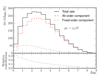
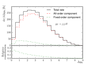
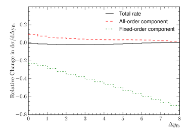
Figure 16: Plots showing the make-up of the cross-section as a function of the rapidity difference between the most forward and backward jets, $\Delta y_{fb}$. The left-hand side shows the composition when the unordered emissions are included only through addition of fixed-order events. The green dotted line is the contribution from all such fixed-order events, the red dashed line is the contribution from the all-order summation, and the black solid line is the sum of the two. The right-hand side plot shows the same results, when the all-order summation is extended to included the unordered emissions. The bottom plot shows the relative change in the fixed-order, all-order and total rate after the extension of the all-order summation. The distributions are discussed further in the text.

The first thing to note on Fig. 16 (top left) is that the relative contribution of the fixed-order component is uniformly decreasing from 30% to 0% for increasing rapidity-spans $\Delta y_{fb}$. This is because the FKL-ordered contributions dominate for large $\Delta y_{fb}$. Secondly, we note that including the unordered emissions in the all-order treatment reduces the impact of the fixed-order matching significantly (as seen by comparing the lower panels of Fig. 16), specifically from roughly 30% to 24% in the bin of lowest rapidity span (where it peaks), and that the approach to 0% is much faster, since the largest sub-leading logarithmic contribution is now included in the all-order approach. Lastly, we note that the sum of the fixed-order and all-order results are largely unchanged after the inclusion of the unordered emissions in the all-order summation: this is seen by the black lines being largely unchanged between the left and right plots. This is made clearer in the bottom plot on Fig. 16, which shows the relative change in the differential cross section for the two components and for the total rate. We see that the total rate is almost unchanged for all $\Delta y_{fb}$. This is in line with the rough expectation, since NLL corrections should amount to a correction of order $\alpha_{s}$ compared to the LL in the relevant channels (and the unordered emissions lead to corrections to only the channels with incoming quarks, not the $gg$-channel). However, the dramatic reduction in the fixed-order component of the cross section starts at about 25% and rises linearly to 70% over the same interval. The increase in the reduction of the fixed-order component is driven by the leading logarithms in the unordered $H+3j$ cross section, which as discussed earlier constitutes part of the sub-leading corrections to $H+3j$. The fact that the reduction is linear in $\Delta y$ is a nice illustration of the dependence on $\log(s/t)\approx\Delta y$ of the component moved from the fixed-order treatment to the all-order component.

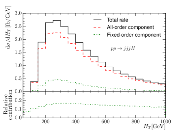
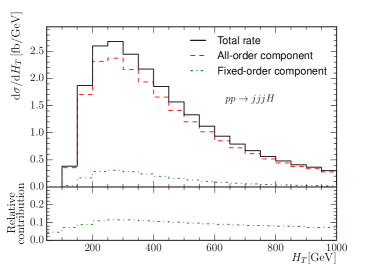
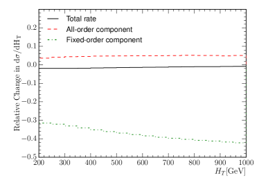
Figure 17: Plots showing the make-up of the cross-section as a function of the total transverse momentum of the event, $H_{T}$. The left-hand side shows the composition when the unordered emissions are included only through addition of fixed-order events. The green dash-dotted line is the contribution from all such fixed-order events, the red dashed line is the contribution from the all-order summation, and the black solid line is the sum of the two. The right-hand side plot shows the same results, when the all-order summation is extended to included the unordered emissions. The distributions are discussed further in the text.

Fig. 17 shows the same information versus $H_{T}$. While $H_{T}$ is not systematically connected with the all-order summation, a large value of $H_{T}$ limits the range of $\Delta y_{fb}$; so as seen on the top left plot (the results when the unordered emissions are left in the fixed-order component), the contribution from the fixed-order component of the cross section increases from 8% to 16% and decreases to around 12% as $H_{T}$ increases from 200 GeV to 1 TeV. The plot at the top right shows the results when the unordered, NLL emissions are included in the all-order treatment, and here the contribution from the fixed-order component is reduced to 4%-12% throughout the range of $H_{T}$, and is below 8% by $H_{T}=1$ TeV.. This shows again that the first NLL terms of the unordered emissions amount to a large portion of the $\mathcal{O}(\alpha_{s}^{5})$-contribution not accounted for by the FKL configurations. As seen on the lower plot, the change in the all-order rate increases slightly from 4% to 5%, while the fixed-order contribution decreases from 32% to 42%, leading to an overall decrease in the total differential rate of a few percent.

As demonstrated in Figs. 16–17, the inclusion of the first NLL terms through the unordered emissions leads to a large systematic reduction in the dependence of the cross section on the matching through the fixed-order component. The inclusion of the unordered emissions and reduction in the dependence on the fixed-order matching is particularly important for studies of the average number of jets versus the rapidity span, as discussed later.

3 Analysis of Results

In this section we will present the predictions which arise from the formalism described in the previous section. The study of the gluon-fusion component of Higgs-boson production in association with dijets is interesting for two separate reasons: firstly, it is a background to the extraction of the measurement of the weak-boson-fusion component, and while both production mechanisms manifest themselves in the Higgs boson+dijet channel, several kinematic distributions and in particular their higher-order corrections differ, and a thorough understanding of these can aid in the suppression of the gluon-fusion-component when the aim is a study of VBF. Secondly, the gluon-fusion component in Higgs boson+dijets can be studied on its own and as such e.g. the azimuthal correlation between the jets can be used for an extraction of the $CP$-structure of the Higgs boson to gluon coupling, even in the case of direct $CP$-violation and mixing in extended Higgs sectors[19, 20, 53]. These two studies would evidently need separate cuts and approaches for event selection, in order to enhance or suppress the gluon-fusion component. For both purposes, the region of phase space with large rapidity span and large dijet invariant mass is of interest.

3.1 Setup and Parameters

In the current investigation we will focus on a few variables from the first experimental analyses[15], except that the predictions presented here will be for the LHC@13TeV. Furthermore, we require that the events contain at least two jets (anti-$k_{T}$ algorithm, $R=0.4$) which satisfy

$$\begin{split}&p_{\perp,j}>30~{}{\rm GeV},\quad|y_{j}|<4.4.\end{split}$$ (60)

Since the weak-boson fusion process is initiated by two quarks, which often carry a large part of the proton momenta, and receive only a modest transverse momentum in the $t$-channel exchange of a weak boson, such events will frequently result in a pair of jets separated by a large invariant mass and rapidity. Following the early analysis of the ATLAS collaboration [15], we will also investigate the gluon-fusion contribution within the VBF-selection cuts applied to the two hardest jets in the event

$$|y_{1}-y_{2}|>2.8,\qquad m_{j_{1}j_{2}}>400~{}\textrm{GeV}.$$ (61)

As already discussed, the radiative corrections for the weak-boson fusion process are significantly smaller than those for the gluon-fusion process. In particular, the contribution from the 3-jet rate is small, and so for the VBF process it is less relevant to distinguish whether the two jets which are asked to fulfil the VBF cuts are also the two hardest jets, the forward-backward jets (which always have the largest rapidity separation, and often the largest invariant mass), or whether one merely requires the existence of at least two jets which fulfil the VBF cuts.

As in [15], we consider Higgs boson decays into two photons with

$$|y_{\gamma}| <2.37,\qquad 105~{}\textrm{GeV}<m_{\gamma_{1}\gamma_{2}}<160~{}\textrm{GeV},$$

$$p_{\perp,\gamma_{1}} >0.35\,m_{\gamma_{1}\gamma_{2}},\qquad p_{\perp,\gamma_{2}}>0.25\,m_{\gamma_{1}\gamma_{2}},$$ (62)

and require the photons to be separated from the jets and each other by $\Delta R(\gamma,j),\Delta R(\gamma_{1},\gamma_{2})>0.4$.

We use the CT14nlo pdf set [54] as provided by LHAPDF6 [55], choosing central renormalisation and factorisation scales of $\mu_{r}=\mu_{f}=H_{T}/2$. To estimate the perturbative uncertainty we also consider all combinations of $\mu_{r},\mu_{f}\in\{H_{T}/4,\sqrt{2}H_{T}/4,H_{T}/2,H_{T}/\sqrt{2},H_{T}\}$ that fulfil $1/2<\mu_{r}/\mu_{f}<2$. Larger ratios of the scales are excluded in order to avoid artificially large logarithms. In the effective $ggH$ coupling in both calculations, we take the limit of an infinite top mass and set the renormalisation scale to the Higgs boson mass.

3.2 Differential Distributions for Higgs Boson Plus Dijets

This subsection will present a comparison of results for the gluon-fusion component of Higgs-boson-plus-dijets from HEJ and from a NLO QCD calculation facilitated by MCFM [56, 57]. We also show leading-order results in order to demonstrate the higher-order effects in both schemes. To avoid visual clutter, we refrain from including the scale-variation uncertainties for the leading-order curves. We start by discussing distributions obtained within the inclusive cuts of Eq. (60) and Eq. (3.1) which will be important for understanding the impact of the VBF cuts in Eq. (61).

Firstly, we find that with the scales choices made, the inclusive cross section for Higgs-boson-plus-dijets at NLO is $6.48^{+0.08}_{-0.57}$ fb, while the result obtained in HEJ is $4.06^{+1.15}_{-0.87}$ fb. The central value found at leading order is $4.41$ fb, and so the result for HEJ for the inclusive cross section for Higgs-boson-plus-dijets is slightly less than the LO value, and the correction compared to LO is in the opposite direction to the result found at NLO. The cross-section obtained at LO is not within the scale variation of the NLO result, and the higher-order corrections are therefore expected to be large.

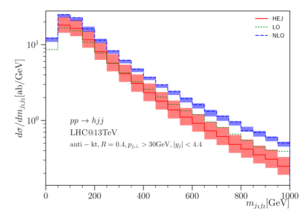
Figure 18: The distribution of the invariant mass between the two hardest jets. Predictions from HEJ are shown in red (full line) while the NLO result is shown in blue (dashed line). The distributions are discussed further in the text.

Fig. 18 shows the distribution in the invariant mass between the two hardest (in transverse momentum) jets within the inclusive cuts. The distribution obtained with HEJ is slightly steeper than that at NLO; we will see below that this is because HEJ allows for more jet radiation than a NLO-calculation, and the samples with more than just two jets carry more relative weight. This in turn means the hardest two jets on average are closer in rapidity and therefore have a smaller invariant mass.

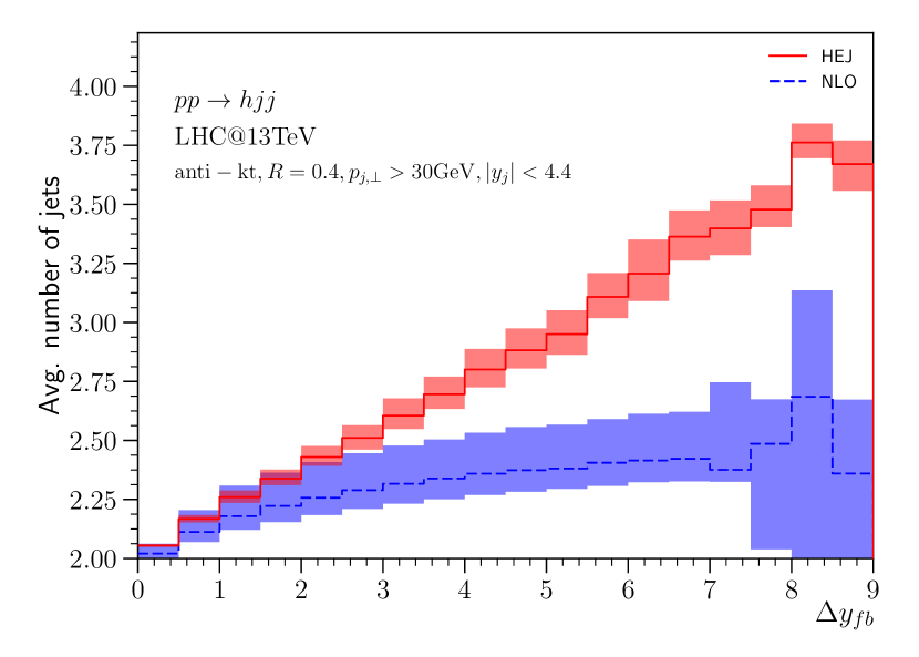
(a)

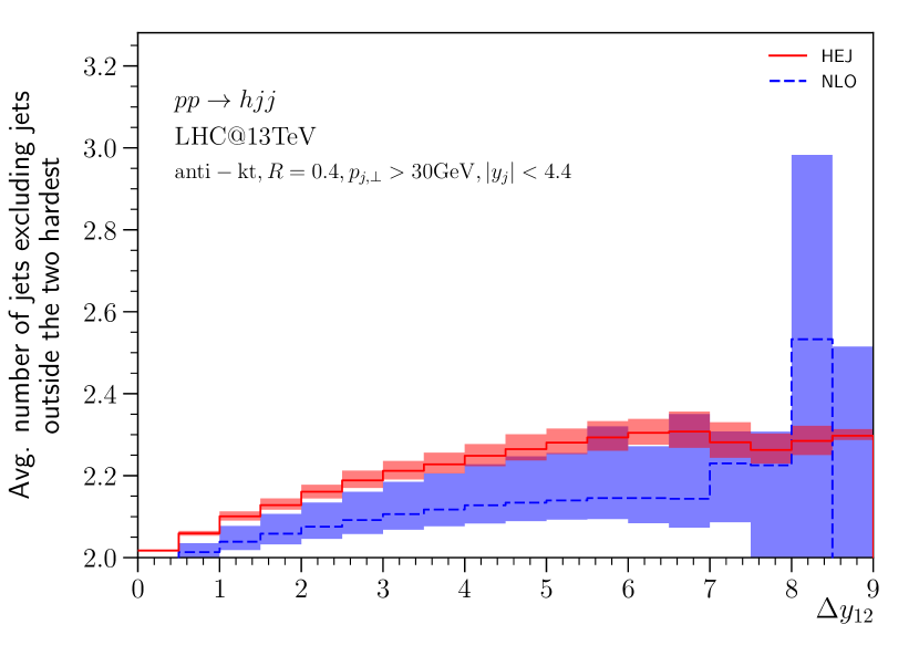
(b)

Figure 19: The average number of jets as a function of the rapidity difference between the most forward and backward jets (a) and between the hardest two jets (b). The HEJ predictions are shown in red while the NLO results are shown in blue (dashed). Both distributions are discussed in the text.

To investigate further the expected impact of the VBF cuts, we calculate the average number of hard jets observed versus the rapidity difference between jets. A successful description of this radiation pattern is necessary for the distinction of the VBF and GF process[21], and in particular for a correct description of the effect of the VBF cuts on the GF component. It is well-known that in all descriptions of dijet processes, and indeed data, the average number of hard jets increases with the rapidity difference between the most forward and backward hard jets, $y_{fb}$. This is clearly seen in the results for both NLO and HEJ in Fig. 19(a). The prediction from HEJ rises more steeply than the equivalent prediction from the NLO calculation, which plateaus at a value of 2.4 already for $\Delta y_{fb}=5$, where the prediction for the exclusive hard 3-jet rate is nearly as large as the exclusive hard 2-jet rate (obviously the NLO calculation for Higgs boson plus dijet production gives an NLO estimate for the dijet rate, but only a LO estimate for the trijet rate). It is indeed expected that HEJ should rise higher than NLO, as the NLO calculation contains only contributions from 2- and 3-jet events and does not contain the all-order evolution in rapidity which is present in HEJ. This steeper dependence obtained in HEJ has been seen to give a good description of data in other dijet processes, where data has already allowed detailed analyses, see e.g. Ref. [24]. Since the contribution from higher jet counts is small in the VBF-process, a large number of jets from the gluon-fusion process would make it easier to distinguish the two. This will be the source of the difference between the prediction of HEJ and NLO for the GF contribution within the VBF-cuts.

Fig. 19(b) shows the average number of hard jets within the same phase space as Fig. 19(a), but as a function of the rapidity separation between the two hardest jets, and not counting jets with rapidities outside the two hardest jets. HEJ has been shown to also give a good description of this observable for other dijet processes[24]. When the jets outside the two hardest ones are excluded, the rise in the average number of hard jets counted is far less for both NLO and HEJ. Indeed, both predictions plateau with a value of roughly 2.2 at around $\Delta y_{12}=6$. The difference between Fig. 19(a) and Fig. 19(b) is caused only by events with three or more jets (since if there are just two, there is no difference between the two hardest jets, and the two furthest apart in rapidity), and thus no large difference between the two observables is expected for the VBF process. The large contribution from the component with 3-jets and higher in the gluon-fusion process means that significant differences can arise in superficially similarly defined quantities as illustrated in Fig. 19. This is important for the use of cuts to suppress the gluon-fusion component in VBF analysis, and separately for the focus on the gluon-fusion component e.g. for the extraction of the $CP$-structure of the $ggH$-coupling.

We will now discuss kinematic distributions of the Higgs-boson and the jets, both for the inclusive and the VBF cuts. The prediction obtained with NLO for the cross-section within the VBF-cuts is $0.87^{+0.02}_{-0.09}$ fb (with LO it is 0.62 fb), and with HEJ it is $0.38^{+0.11}_{-0.08}$ fb. We argue that for the VBF-cuts the results obtained with HEJ are more reliable than those obtained with NLO. This is because a successful description of the VBF-cuts relies on the description of the emission of further hard jets from the production of Higgs-boson plus dijets. Even at the Tevatron centre-of-mass energy of 1.96 TeV, the pure NLO-calculation gives an insufficient description of the average number of jets in other dijet-processes such as W+dijets. This deficiency of the NLO-calculation will be even larger at the LHC, whereas HEJ gives a good description of the hard jet-production in other processes with similar jet-cuts as those applied in this study of Higgs-boson production with dijets.

In Fig. 20(a), we show the Higgs transverse momentum distribution within the cuts of Eq. (60), while Fig. 20(b) is the same distribution when also the VBF cuts of Eq. (61) are fulfilled. We observe the understood reduction in cross-section obtained with HEJ compared to NLO. The two peaks visible in the LO obtained within the VBF cuts are caused by the azimuthal structure of the $ggH$ coupling. As we will see later, the cross-section peaks when the jets are back-to-back and has another local maximum when they are collinear. This induces the two features in the LO curves, which become broader and indistinguishable when further radiation is included through either the NLO corrections or the all-order summation.

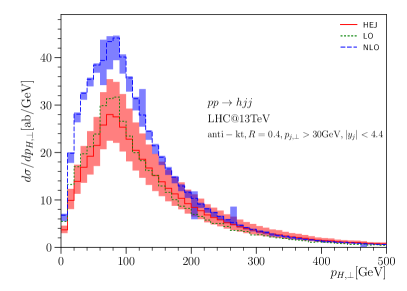
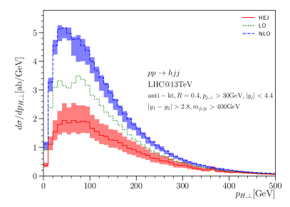
(a)                                                          (b)

Figure 20: (a) The transverse momentum distribution of the Higgs boson in inclusive dijet events, and (b) when the hardest two jets are required to pass the VBF-cuts. Predictions from HEJ are shown in red while the NLO result is shown in blue. Both distributions are discussed further in the text.

The radiative corrections at NLO are found to be large for the gluon-fusion component of Higgs-plus-dijets; in particular, the 3-jet component forms a significant part of the 2-jet cross section at NLO — contrary to the situation for the VBF component. Furthermore the one-loop interference between the QCD and EW component is negligible[12]. Requiring that the two hardest jets are separated in rapidity and invariant mass according to Eq. (61) reduces the gluon fusion component more compared to just requiring the existence of two jets which satisfy the requirement. Other selection processes may be of significance for the study of the gluon-fusion component alone, and will be the focus of further studies. We note again here that the application of the further VBF cuts reduces the gluon-fusion cross section from $6.48$ fb (inclusive) to $0.87$ fb (VBF cuts) at NLO and from $4.06$ fb to $0.38$ fb in the HEJ resummation. This corresponds to a severe reduction of the HEJ cross section to $9.4\%$, whereas NLO QCD predicts a reduction to $13.4\%$ of the inclusive cross section, and the difference is explained by the deficiency of a NLO-calculation in describing the number of hard jets produced by the gluon-fusion process in the VBF-region of phase space.

We also note that the transverse momentum distribution for the Higgs boson is relatively hard such that the effective theory derived from $m_{t}\to\infty$ will obviously not apply in all the relevant region, but the results presented here are still relevant for inspecting the impact of the high-energy summation. Furthermore, the $m_{t}\to\infty$-limit and the high-energy limits commute, and the leading high-energy effects can be calculated with full top-mass dependence. This is the focus of ongoing work within HEJ.

A tree-level analysis indicates that the $CP$ structure of the Higgs coupling can be cleanly studied using the azimuthal angle between the two jets[19], with the definition of the azimuthal angle extended to the full range $[-\pi;\pi]$ by e.g. always measuring it counter-clockwise relative to a predefined forward direction. The Born-level analysis of the Standard Model couplings predicts an even, cosine-like behaviour, and the extension of the azimuthal angle to the full range of $-\pi$ to $\pi$ allows for a probe of $CP$ admixtures[19]. In Fig. 21, we show the distribution of the angle between the hardest two jets, $\phi_{j_{1}j_{2}}$ with (a) inclusive and (b) VBF cuts. We again see the same reduction in cross section of HEJ compared to the NLO prediction. The shape around $\phi_{j_{1}j_{2}}=0$ in Fig. 21(a) is caused by the removal of tree-level three-parton events which appear in two-jet configurations — the extension of the dip is determined by the $R$-parameter in the jet-clustering, which removes the contribution arising from collinear splittings of 2-jet events.

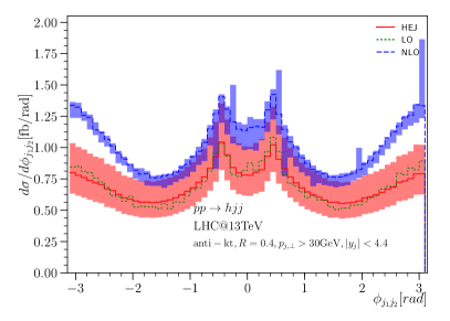
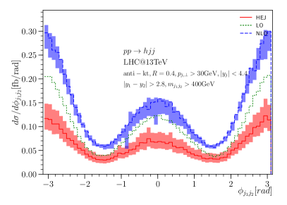
(a)                                                          (b)

Figure 21: (a) The distribution of the azimuthal angle between the two hardest jets, $\phi_{j_{1}j_{2}}$, and (b) ditto within the VBF cuts. The cosine-like even distribution is a finger-print of the $CP$-even structure of the $ggH$-vertex. Predictions from HEJ are shown in red (solid line) while the NLO result is shown in blue (dashed).

We have therefore seen in this section that higher-order corrections in Higgs-boson-plus-dijet production are large and have a significant impact on the results of imposing VBF event selection cuts.

4 Conclusions

In this paper we have described the production of a Higgs boson with at least two jets within the High Energy Jets (HEJ) formalism. This key process will be central to efforts to pin down properties of the Higgs couplings to vector bosons. We implemented the process of Higgs-boson production in association with at least two jets within the framework of HEJ. Furthermore, we calculated the first next-to-leading logarithmic corrections to the framework by including the un-ordered emission of a gluon (i.e. the emission of gluon outside of the rapidity region contributing to the leading-logarithmic behaviour of the cross section) in the all-order treatment for the first time. Such regions were previously accounted for only through matching to fixed-order matrix-elements. The new results increases the fraction of the total cross section which is controlled by HEJ and subject to resummation, while also reducing our dependence on fixed-order matching.

We have then studied the predicted jet radiation patterns for various distributions within typical experimental cuts, and compared these to the corresponding results for a fixed-order NLO calculation. The inclusion of higher-order corrections beyond NLO are clearly observed in the average number of jets as a function of rapidity, where other variables show less pronounced differences. This result can be used to distinguish the gluon-fusion and vector-boson fusion component of the Higgs boson+dijet cross section.

We have also seen that imposing topological “VBF” cuts has a significant impact on the cross section beyond that predicted at NLO (for the particular choice here, the cross section was reduced to $9.4$% of the original). This is understood as a combination of increased jet activity in any event with a reasonable rapidity separation and the impact of the all-order virtual corrections included in the HEJ description.

Appendix A Tree-Level Amplitudes for $qg\to qg$

A short calculation gives the amplitude for the process $qg\to qg$. We use the following notation for spinors:

$$\begin{split}u_{\pm}(p)=|p\pm\rangle,\qquad\overline{u}_{\pm}(p)=\langle p\pm|,\\ \langle{pk}\rangle=\langle p-|k+\rangle=\overline{u}_{-}(p)u_{+}(k),\\ [{pk}]=\langle p+|k-\rangle=\overline{u}_{+}(p)u_{-}(k),\end{split}$$ (63)

and then find for $q^{-}(p_{a})+g^{-}(p_{b})\to q^{-}(p_{1})+g^{-}(p_{2})$

$$i\mathcal{M}_{qg\to qg}=2ig^{2}\left(t^{2}_{1e}t^{b}_{ea}\frac{\langle 2a\rangle\langle 12\rangle^{2}}{\langle a1\rangle\langle 2b\rangle\langle ba\rangle}+t^{b}_{1e}t^{2}_{ea}\frac{[ab]^{3}}{[1a][a2][2b]}\right).$$ (64)

The factors of $t^{X}_{MN}$ are fundamental colour matrices; where an index is one of $\{a,b,1,2\}$, it represents the index associated with that particle. Repeated indices are summed over.

We now wish to consider the behaviour of this expression in the HE limit. Without loss of generality, we take $p_{a}$ to be in the incoming positive direction and $p_{b}$ to be in the incoming negative direction. We consider first the configuration that is consistent with FKL-ordering such that $y_{1}\gg y_{2}$. The magnitude of each spinor product $\langle ij\rangle$ or $[ij]$ is given by the square root of the magnitude of the corresponding invariant:

$$|\langle ij\rangle|=\sqrt{|s_{ij}|}=|[ij]|.$$ (65)

Therefore in this configuration, for example, $|[ab]|=\sqrt{s}\to\infty$ in the HE limit and $|[b2]|=\sqrt{-t}$ remains finite. We therefore find that both terms in Eq. (64) scale as $s/t$, and in particular that the $s$-dependence is $s^{1}$ in agreement with Regge theory.

Alternatively, if we take $y_{2}\gg y_{1}$, this means that $t=(p_{2}-p_{a})^{2}$ such that $\langle b1\rangle$ scales like $\sqrt{-t}$ while $\langle b2\rangle$ now scales like $\sqrt{s}$. Therefore the terms in Eq. (64) now scale as $\sqrt{t/s}$ and $\sqrt{s/t}$ respectively. The dominant behaviour in the HE limit is therefore $\sqrt{s/t}$, again in agreement with Regge theory.

We have chosen a particular helicity assignment here. The analogous expression for $q^{-}(p_{a})+g^{+}(p_{b})\to q^{-}(p_{1})+g^{+}(p_{2})$ is

$$i\mathcal{M}_{qg\to qg}=-2ig^{2}\left(t^{2}_{1e}t^{b}_{ea}\frac{[a2]^{3}}{[1a][ab][b2]}+t^{b}_{1e}t^{2}_{ea}\frac{\langle ba\rangle\langle 1b\rangle^{2}}{\langle 1a\rangle\langle a2\rangle\langle 2b\rangle}\right).$$ (66)

Again, in the FKL configuration both terms scale as $s/t$. However, in this case in the non-FKL configuration neither term contributes a leading $\sqrt{s/t}$ term, and instead yield $\sqrt{t^{3}/s^{3}}$ and $\sqrt{t/s}$ respectively. The other two non-zero helicity configurations may be obtained by complex conjugation.

References

- [1] ATLAS Collaboration, G. Aad et al., Observation of a new particle in the search for the Standard Model Higgs boson with the ATLAS detector at the LHC, Phys.Lett. B716 (2012) 1–29, [arXiv:1207.7214].
- [2] CMS Collaboration, S. Chatrchyan et al., Observation of a new boson at a mass of 125 GeV with the CMS experiment at the LHC, Phys.Lett. B716 (2012) 30–61, [arXiv:1207.7235].
- [3] ATLAS Collaboration Collaboration, G. Aad et al., Evidence for the spin-0 nature of the Higgs boson using ATLAS data, Phys.Lett. B726 (2013) 120–144, [arXiv:1307.1432].
- [4] ATLAS Collaboration Collaboration, G. Aad et al., Measurements of Higgs boson production and couplings in diboson final states with the ATLAS detector at the LHC, Phys.Lett. B726 (2013) 88–119, [arXiv:1307.1427].
- [5] ATLAS Collaboration Collaboration, G. Aad et al., Measurement of the Higgs boson mass from the and channels with the ATLAS detector using 25 fb-1 of collision data, Phys.Rev. D90 (2014) 052004, [arXiv:1406.3827].
- [6] ATLAS Collaboration Collaboration, G. Aad et al., Measurements of Higgs boson production and couplings in the four-lepton channel in pp collisions at center-of-mass energies of 7 and 8 TeV with the ATLAS detector, arXiv:1408.5191.
- [7] ATLAS Collaboration Collaboration, G. Aad et al., Measurement of Higgs boson production in the diphoton decay channel in collisions at center-of-mass energies of 7 and 8 TeV with the ATLAS detector, arXiv:1408.7084.
- [8] CMS Collaboration Collaboration, S. Chatrchyan et al., Study of the Mass and Spin-Parity of the Higgs Boson Candidate Via Its Decays to Z Boson Pairs, Phys.Rev.Lett. 110 (2013) 081803, [arXiv:1212.6639].
- [9] CMS Collaboration Collaboration, S. Chatrchyan et al., Measurement of the properties of a Higgs boson in the four-lepton final state, Phys.Rev. D89 (2014) 092007, [arXiv:1312.5353].
- [10] CMS Collaboration Collaboration, V. Khachatryan et al., Constraints on the Higgs boson width from off-shell production and decay to Z-boson pairs, Phys.Lett. B736 (2014) 64, [arXiv:1405.3455].
- [11] CMS Collaboration Collaboration, V. Khachatryan et al., Observation of the diphoton decay of the Higgs boson and measurement of its properties, arXiv:1407.0558.
- [12] J. R. Andersen, T. Binoth, G. Heinrich, and J. M. Smillie, Loop induced interference effects in Higgs Boson plus two jet production at the LHC, JHEP 0802 (2008) 057, [arXiv:0709.3513].
- [13] A. Bredenstein, K. Hagiwara, and B. Jäger, Mixed QCD-electroweak contributions to Higgs-plus-dijet production at the LHC, Phys.Rev. D77 (2008) 073004, [arXiv:0801.4231].
- [14] L. J. Dixon and Y. Sofianatos, Analytic one-loop amplitudes for a Higgs boson plus four partons, JHEP 0908 (2009) 058, [arXiv:0906.0008].
- [15] ATLAS Collaboration Collaboration, G. Aad et al., Measurements of fiducial and differential cross sections for Higgs boson production in the diphoton decay channel at TeV with ATLAS, arXiv:1407.4222.
- [16] ATLAS Collaboration Collaboration, G. Aad et al., Fiducial and differential cross sections of Higgs boson production measured in the four-lepton decay channel in collisions at =8 TeV with the ATLAS detector, arXiv:1408.3226.
- [17] V. Del Duca, W. Kilgore, C. Oleari, C. Schmidt, and D. Zeppenfeld, Higgs + 2 jets via gluon fusion, Phys.Rev.Lett. 87 (2001) 122001, [hep-ph/0105129].
- [18] V. Del Duca, W. Kilgore, C. Oleari, C. Schmidt, and D. Zeppenfeld, Gluon fusion contributions to H + 2 jet production, Nucl.Phys. B616 (2001) 367–399, [hep-ph/0108030].
- [19] G. Klämke and D. Zeppenfeld, Higgs plus two jet production via gluon fusion as a signal at the CERN LHC, JHEP 0704 (2007) 052, [hep-ph/0703202].
- [20] J. R. Andersen, K. Arnold, and D. Zeppenfeld, Azimuthal Angle Correlations for Higgs Boson plus Multi-Jet Events, JHEP 1006 (2010) 091, [arXiv:1001.3822].
- [21] Y. L. Dokshitzer, V. A. Khoze, and T. Sjöstrand, Rapidity gaps in Higgs production, Phys.Lett. B274 (1992) 116–121.
- [22] ATLAS Collaboration Collaboration, G. Aad et al., Measurement of dijet production with a veto on additional central jet activity in collisions at TeV using the ATLAS detector, JHEP 1109 (2011) 053, [arXiv:1107.1641].
- [23] ATLAS Collaboration Collaboration, G. Aad et al., Measurements of jet vetoes and azimuthal decorrelations in dijet events produced in collisions at = 7 TeV using the ATLAS detector, arXiv:1407.5756.
- [24] D0 Collaboration, V. M. Abazov et al., Studies of boson plus jets production in collisions at TeV, Phys.Rev. D88 (2013) 092001, [arXiv:1302.6508].
- [25] V. S. Fadin, E. A. Kuraev, and L. N. Lipatov, On the Pomeranchuk singularity in asymptotically free theories, Phys. Lett. B60 (1975) 50–52.
- [26] E. A. Kuraev, L. N. Lipatov, and V. S. Fadin, Multi - Reggeon processes in the Yang-Mills theory, Sov. Phys. JETP 44 (1976) 443–450.
- [27] E. A. Kuraev, L. N. Lipatov, and V. S. Fadin, The Pomeranchuk singularity in nonabelian gauge theories, Sov. Phys. JETP 45 (1977) 199–204.
- [28] I. I. Balitsky and L. N. Lipatov, The Pomeranchuk singularity in quantum chromodynamics, Sov. J. Nucl. Phys. 28 (1978) 822–829.
- [29] ATLAS Collaboration Collaboration, G. Aad et al., Measurements of the W production cross sections in association with jets with the ATLAS detector, arXiv:1409.8639.
- [30] J. R. Andersen and J. M. Smillie, Constructing All-Order Corrections to Multi-Jet Rates, JHEP 1001 (2010) 039, [arXiv:0908.2786].
- [31] J. R. Andersen and J. M. Smillie, The Factorisation of the t-channel Pole in Quark-Gluon Scattering, Phys.Rev. D81 (2010) 114021, [arXiv:0910.5113].
- [32] J. R. Andersen and J. M. Smillie, Multiple Jets at the LHC with High Energy Jets, JHEP 1106 (2011) 010, [arXiv:1101.5394].
- [33] J. R. Andersen, T. Hapola, and J. M. Smillie, W Plus Multiple Jets at the LHC with High Energy Jets, JHEP 1209 (2012) 047, [arXiv:1206.6763].
- [34] J. R. Andersen, J. J. Medley, and J. M. Smillie, plus multiple hard jets in high energy collisions, JHEP 05 (2016) 136, [arXiv:1603.0546].
- [35] CMS Collaboration Collaboration, S. Chatrchyan et al., Measurement of the inclusive production cross sections for forward jets and for dijet events with one forward and one central jet in collisions at TeV, JHEP 1206 (2012) 036, [arXiv:1202.0704].
- [36] S. Catani, F. Krauss, R. Kuhn, and B. Webber, QCD matrix elements + parton showers, JHEP 0111 (2001) 063, [hep-ph/0109231].
- [37] L. Lönnblad, ARIADNE version 4: A Program for simulation of QCD cascades implementing the color dipole model, Comput.Phys.Commun. 71 (1992) 15–31.
- [38] R. Brower, C. E. DeTar, and J. Weis, Regge Theory for Multiparticle Amplitudes, Phys.Rept. 14 (1974) 257.
- [39] V. S. Fadin, R. Fiore, M. G. Kozlov, and A. V. Reznichenko, Proof of the multi-Regge form of QCD amplitudes with gluon exchanges in the NLA, Phys. Lett. B639 (2006) 74–81, [hep-ph/0602006].
- [40] J. Alwall, R. Frederix, S. Frixione, V. Hirschi, F. Maltoni, O. Mattelaer, H. S. Shao, T. Stelzer, P. Torrielli, and M. Zaro, The automated computation of tree-level and next-to-leading order differential cross sections, and their matching to parton shower simulations, JHEP 07 (2014) 079, [arXiv:1405.0301].
- [41] V. Del Duca, Equivalence of the Parke-Taylor and the Fadin-Kuraev-Lipatov amplitudes in the high-energy limit, Phys.Rev. D52 (1995) 1527–1534, [hep-ph/9503340].
- [42] S. J. Parke and T. Taylor, An Amplitude for Gluon Scattering, Phys.Rev.Lett. 56 (1986) 2459.
- [43] V. Del Duca, Parke-Taylor amplitudes in the multi - Regge kinematics, Phys. Rev. D48 (1993) 5133–5139, [hep-ph/9304259].
- [44] A. V. Bogdan and V. S. Fadin, A proof of the reggeized form of amplitudes with quark exchanges, Nucl. Phys. B740 (2006) 36–57, [hep-ph/0601117].
- [45] V. S. Fadin, M. G. Kozlov, and A. V. Reznichenko, Radiative corrections to QCD amplitudes in quasi-multi-Regge kinematics, Phys. Atom. Nucl. 67 (2004) 359–375, [hep-ph/0302224].
- [46] V. S. Fadin, The gluon Reggeization in perturbative QCD at NLO, hep-ph/0511121.
- [47] V. S. Fadin and L. N. Lipatov, Next-to-leading corrections to the BFKL equation from the gluon and quark production, Nucl. Phys. B477 (1996) 767–808, [hep-ph/9602287].
- [48] A. Bogdan, V. Del Duca, V. S. Fadin, and E. N. Glover, The Quark Regge trajectory at two loops, JHEP 0203 (2002) 032, [hep-ph/0201240].
- [49] V. Del Duca, A. Frizzo, and F. Maltoni, Factorization of tree QCD amplitudes in the high-energy limit and in the collinear limit, Nucl.Phys. B568 (2000) 211–262, [hep-ph/9909464].
- [50] V. Del Duca, W. Kilgore, C. Oleari, C. Schmidt, and D. Zeppenfeld, Kinematical limits on Higgs boson production via gluon fusion in association with jets, Phys.Rev. D67 (2003) 073003, [hep-ph/0301013].
- [51] J. R. Andersen and C. D. White, A New Framework for Multijet Predictions and its application to Higgs Boson production at the LHC, Phys. Rev. D78 (2008) 051501, [arXiv:0802.2858].
- [52] J. R. Andersen, V. Del Duca, and C. D. White, Higgs Boson Production in Association with Multiple Hard Jets, JHEP 02 (2009) 015, [arXiv:0808.3696].
- [53] M. J. Dolan, P. Harris, M. Jankowiak, and M. Spannowsky, Constraining -violating Higgs Sectors at the LHC using gluon fusion, Phys. Rev. D90 (2014) 073008, [arXiv:1406.3322].
- [54] S. Dulat, T.-J. Hou, J. Gao, M. Guzzi, J. Huston, P. Nadolsky, J. Pumplin, C. Schmidt, D. Stump, and C. P. Yuan, New parton distribution functions from a global analysis of quantum chromodynamics, Phys. Rev. D93 (2016), no. 3 033006, [arXiv:1506.0744].
- [55] A. Buckley, J. Ferrando, S. Lloyd, K. Nordström, B. Page, M. Rüfenacht, M. Schönherr, and G. Watt, LHAPDF6: parton density access in the LHC precision era, Eur. Phys. J. C75 (2015) 132, [arXiv:1412.7420].
- [56] J. M. Campbell, R. K. Ellis, and G. Zanderighi, Next-to-Leading order Higgs + 2 jet production via gluon fusion, JHEP 0610 (2006) 028, [hep-ph/0608194].
- [57] J. M. Campbell, R. K. Ellis, and C. Williams, Hadronic production of a Higgs boson and two jets at next-to-leading order, Phys.Rev. D81 (2010) 074023, [arXiv:1001.4495].