Semantic Vector Encoding and Similarity Search Using Fulltext Search Engines

Abstract

Vector representations and vector space modeling (VSM) play a central role in modern machine learning. We propose a novel approach to ‘vector similarity searching’ over dense semantic representations of words and documents that can be deployed on top of traditional inverted-index-based fulltext engines, taking advantage of their robustness, stability, scalability and ubiquity. We show that this approach allows the indexing and querying of dense vectors in text domains. This opens up exciting avenues for major efficiency gains, along with simpler deployment, scaling and monitoring. The end result is a fast and scalable vector database with a tunable trade-off between vector search performance and quality, backed by a standard fulltext engine such as Elasticsearch. We empirically demonstrate its querying performance and quality by applying this solution to the task of semantic searching over a dense vector representation of the entire English Wikipedia.

1 Introduction

The vector space model Salton et al. (1975) of representing documents in high-dimensional vector spaces has been validated by decades of research and development. Extensive deployment of inverted-index-based information retrieval (IR) systems has led to the availability of robust open source IR systems such as Sphinx, Lucene or its popular, horizontally scalable extensions of Elasticsearch and Solr.

Representations of document semantics based solely on first order document-term statistics, such as TF-IDF or Okapi BM25, are limited in their expressiveness and search recall. Today, approaches based on distributional semantics and deep learning allow the construction of semantic vector space models representing words, sentences, paragraphs or even whole documents as vectors in high-dimensional spaces Deerwester et al. (1990); Blei et al. (2003); Mikolov et al. (2013).

The ubiquity of semantic vector space modeling raises the challenge of efficient searching in these dense, high-dimensional vector spaces. We would naturally want to take advantage of the design and optimizations behind modern fulltext engines like Elasticsearch so as to meet the scalability and robustness demands of modern IR applications. This is the research challenge addressed in this paper.

The rest of the paper describes novel ways of encoding dense vectors into text documents, allowing the use of traditional inverted index engines, and explores the trade-offs between IR accuracy and speed. Being motivated by pragmatic needs, we describe the results of experiments carried out on real datasets measured on concrete, practical software implementations.

2 Semantic Vector Encoding for Inverted-Index Search Engines

2.1 Related Work

The standard representation of documents in the Vector Space Model (VSM) Salton and Buckley (1988) uses term feature vectors of very high dimensionality. To map the feature space onto a smaller and denser latent semantic subspace, we may use a body of techniques, including Latent Semantic Analysis (LSA) Deerwester et al. (1990), Latent Dirichlet Allocation (LDA) Blei et al. (2003) or the many variants of Locality-sensitive hashing (LSH) Gionis et al. (1999).

Throughout the long history of VSM developments, many other methods for improving search efficiency have been explored. Weber et al. ran one of the first rigorous studies that dealt with the ineffectiveness of the VSM and the so-called curse of dimensionality. They evaluated several data partitioning and vector approximation schemes, achieving significant nearest-neighbour search speedup in  Weber and Böhm (2000). The scalability of similarity searching through a new index data structures design is described in Zezula et al. (2006). Dimensionality reduction techniques proposed in Digout et al. (2004) allow a robust speedup while showing that not all features are equally discriminative and have a different impact on efficiency, due to their density distribution. Boytsov shows that the $k$-NN search can be a replacement for term-based retrieval when the term-document similarity matrix is dense.

Recently, deep learning approaches and tools like doc2vec Le and Mikolov (2014) construct semantic representations of documents $D$ as $d=|D|$ (dense) vectors in an $n$-dimensional vector space.

To take advantage of ready-to-use and optimized systems for term indexing and searching, we have developed a method for representing points in a semantic vector space encoded as plain text strings. In our experiments, we will be using Elasticsearch Gormley and Tong (2015) in its ‘vanilla’ setup. We do not utilize any advanced features of Elasticsearch, such as custom scoring, tokenization or a $n$-gram analyzers. Thus, our method does not depend on any functionality that is specific to Elasticsearch, and it is possible (and sometimes even desirable) to substitute Elasticsearch with other fulltext engine implementations.

2.2 Our Vector to String Encoding Method

Let our query be a document, represented by its vector $\vec{q}$, for which we aim to find the top $k$ most similar documents in $D$. We want to search efficiently, indexing and deleting documents from the index in near-real-time, and in a manner that could scale by eventual parallelization, re-using the significant research and engineering effort that went into designing and implementing systems like Elasticsearch.

Conceptually, our method consists of encoding vector features into string tokens (feature tokens), creating a text document from each dense vector. These encoded documents are consequently indexed in traditional inverted-index-based search engines. At query time, we encode the query vector and retrieve the subset of similar vectors $E$, $|E|\ll|D|$, using the engine’s fulltext search functionality. Finally, the small set of candidate vectors $E$ is re-ranked by calculating the exact similarity metric (such as cosine similarity) to the query vector. This makes the search effectively a two-phase process, with our encoded fulltext search as the first phase and candidate re-ranking as the second.

2.2.1 Encoding Vectors

The core of our method of encoding vectors into strings lies in encoding the vector feature values at a selected precision as character strings – feature tokens. This is best demonstrated on a small example: Let us take a semantic vector of three dimensions, $\vec{w}=[0.12,-0.13,0.065]$. Each feature token starts with its feature identification (e.g. a feature number such as 0, 1 etc.) followed by a precision encoding schema identifier (such as P2, I10 etc.) and the encoded feature value (such as i0d12, ineg0d2 etc.) depending on the particular encoding method. We propose and evaluate three encoding methods:

rounding

Feature values are rounded to a fixed number of decimal positions and stored as a string that encodes both the feature identification and its value. Rounding to two decimal places produces representation of $\vec{w}$ as [’0P2i0d12’, ’1P2ineg0d13’, ’2P2i0d07’].

interval

quantizes $\vec{w}$ into intervals of fixed length. For example, with an interval width of $0.1$, feature values fall into intervals starting at 0.1, $-0.2$ and 0.0, which we encode as d1, d2 and d0, respectively. Combined with the interval length denotation of I10, the full vector is encoded into the tokens $\vec{w}=[$’0I10i0d1’, ’1I10ineg0d2’, ’2I10i0d0’].

combined

Rounding and interval encoding used together. Rounding $\vec{w}$ to three decimal places and using intervals of length $0.2$, we get the representation of $\vec{w}$ as feature tokens [’0P3i0d120’, ’1P3ineg0d130’, ’2P3i0d065’, ’0I5i0d0’, ’1I5ineg0d2’, ’2I5i0d0’].

The intuition behind all these encoding schemes is a trade-off between increasing feature sparsity and retaining search quality: we show that some types of sparsification actually lead to little loss of quality, allowing an efficient use of inverted-index IR engines.

2.2.2 High-Pass Filtering Techniques

The rationale behind the next two techniques is to filter out semantic vector features of low importance, further increasing feature sparsity. This improves performance at the expense of quality.

Trim:

In the trimming phase, a fixed threshold – such as 0.1 – is used. Feature tokens in the query with an absolute value of the feature below the threshold are simply discarded from the query. In the case of our example vector $\vec{w}=[0.12,-0.13,0.065]$, the tokens representing the third feature value 0.065 are removed since $|0.065|<0.1$.

Best:

Features of each vector are ordered according to their absolute value and only a fixed number of the highest-valued features are added to the index, discarding the rest. As an example, with $best=1$, only the second feature of $-0.13$ (the highest absolute value) would be considered from $\vec{w}$.

Note that in both cases, this type of filtering is only meaningful when the feature ranges are comparable. In our experiments all vectors are normalized to unit length, ranging absolute values of features from zero (no feature importance) to one (maximal feature importance).

2.3 Space and Time Requirements

In this section we summarize and compare the theoretical space and time requirements of our proposed vector-to-string encoding and filtering methods with a baseline of a naive, linear brute force search. The inverted-index-based analysis is based on the documentation of the Lucene search engine implementation.

While the running time of the naive search is stable and predictable, the efficiency of the other optimization methods depends on the data set, such as its vocabulary size and the expected postings list sparsity, after the feature token encoding and filtering. On the other hand, performance can be influenced by how the method is configurated – for example, the expected number of distinct feature values depends on the precision of the rounding of the feature values that was used.

The efficiency trade-offs are summarized in Table 1. Each document is represented as a vector $\vec{d}$ of $n$ features computed by LSA over TF-IDF.

Baseline – naive brute force search:

The naive baseline method avoids using a fulltext search altogether, and instead stores all $d$ ‘indexed’ vectors in their original dense vector representation in RAM, as an $n\times d$ matrix. At query time, it computes a similarity between the query vector $\vec{q}$ and each of the indexed document vectors $\vec{d}$, in a single linear scan through the matrix, and returns the top $k$ vectors with the best score.

Efficiency of a naive brute force search:

The index is a matrix of floats of size $nd$ resulting in $\mathcal{O}(nd)$ space complexity. We have chosen the cosine similarity as our similarity metric. To calculate cossim between the query and all $d$ documents, vector $\vec{q}$ of length $n$ has to be multiplied with a length-normalized matrix of dimensionality $n\times d$, e.g. $\mathcal{O}(nd)$. Using the resulting vector of $d$ scores, we then pick the $k$ nearest documents as the final query result, in $\mathcal{O}(d)$.

Efficiency of encoding:

We investigate the efficiency of our vector-to-string encoding when a general inverted-index-based search engine is used to index and search through them.

At worst, we store one token per dimension for each vector. We need $\mathcal{O}(nd)$ space to store all indexed documents, as is the case with the naive search. In practice, there are several different constants as naive search saves one float per feature (four bytes), while our feature tokens are compressed string-encoded feature values and indices of the sparse feature positions in the inverted index.

Each dimension of the query vector $\vec{q}$ contains a string-encoded feature $q_{j}$. For each $q_{j}$ we fetch a list of documents $c_{i}$ together with term frequency $t_{n}$ in that document: $\operatorname{tf}(t_{n},c_{i})$.

For each of these $(c_{i},\operatorname{tf}(t_{n},c_{i}))$ pairs we add the corresponding score value to the score of document $c_{i}$ in a list of result-candidate documents. The score computation contains a vector dot-product operation in the dimension of the size $v$ of feature vocabulary $V$ that can be computed in $\mathcal{O}(v)$. Document $c_{i}$ is added to the set $C$ of all result-candidate documents, which we sort in $\mathcal{O}(c\log{c})$ time and return the top $k$ results. The whole search is performed in $\mathcal{O}(n\cdot p\cdot v+c\log{c})$ steps, where $p$ is the expected postings list size and $c=|C|$.

Efficiency of high-pass filtering:

We approximate the full feature vector by storing only the most significant features, e.g. only the top $m$ dimensions. When compared with a naive search, we save on space: only $\mathcal{O}(md)$, $m\ll n$ values are needed.

For each feature value $q_{j}$ we have to find all documents with the same feature value. We are able to find the feature set in $\mathcal{O}(\log{j})$ steps, where $j$ is the number of distinct indexed values of the feature. Consequently, we retrieve the matched documents in $\mathcal{O}(l)$ time, where $l$ is the number of documents in the index with the appropriate feature value.

Each of the found documents is added to set $C$ and its score is incremented for this hit. If represented with an appropriate data structure, such as a hash table, we are able to add and increment scores of the items in $\mathcal{O}(1)$ time. Having all $c=|C|$ candidate documents over all the separate feature-searches, we pick and return the top $k$ items in $\mathcal{O}(c)$ time.

Combined, $\mathcal{O}(n\cdot(\log{j}+l)+c)$ steps are needed for the search, where $j$ is the expected number of distinct indexed values per feature and $l$ is the number of documents in the index per feature value.

Table 1: Comparison of encoding methods in terms of space and time. $n$ is the number of semantic vector features, $d$ is the number of semantic vectors, $m$ is the number of semantic vector features after high-pass filtering, $p$ is the expected postings list size (inverted index sparsity), $v$ is the expected vocabulary size per a feature, $c$ is the number of result-candidate semantic vectors, $j$ the expected number of distinct indexed values of the feature, and $l$ the expected number of documents in the index per a feature value. For details see Section 2.3.

	naive search	token encoding	high-pass filtering
space	$\mathcal{O}(nd)$	$\mathcal{O}(nd)$	$\mathcal{O}(md)$
time	$\mathcal{O}(nd)$	$\mathcal{O}(n\cdot p\cdot v+c\log{c})$	$\mathcal{O}(n\cdot(\log{j}+l)+c)$

3 Experimental Setup

To evaluate our method, we used ScaleText Rygl et al. (2016) based on Elasticsearch Gormley and Tong (2015) as our fulltext IR system. The evaluation dataset was the whole of the English Wikipedia consisting of 4,181,352 articles.

3.1 Quality Evaluation

The aim of the quality evaluation was to investigate how well the approximate ‘encoded vector’ search performs in comparison with the exact naive brute-force search, using cosine similarity as the similarity metric. Cosine similarity is definitely not the only possible metric – we selected cosine similarity as we needed a fully automatic evaluation, without any need of human judgement, and because cosine similarity suits our upstream application logic perfectly.

We converted all Wikipedia documents into vectors using LSA with 400 features. We then randomly selected 1,000 documents from our Wikipedia dataset to act as our query vectors. By doing a naive brute force scan over all the vectors (the whole dataset), we identified the 10 most similar ones for each query vector. This became our ‘gold standard’.

We encoded the dataset vectors into various string representations, as described in Section 2.2.1 and stored them in Elasticsearch.

For evaluating the search, we pruned the values in the query vectors (see Section 2.2.2) and encoded them into a string representation. Using these strings, we performed 1,000 Elasticsearch searches. For each query, we measured the overlap between the retrieved documents and the gold standard using Precision@k or the Normalized Discounted Cumulative Gain (nDCG_k). The mean cumulative loss between the ideal and the actual cosine similarities of the top $k$ results (avg. diff.) is also reported.

Note that since we re-rank $|E|$ results obtained from Elasticsearch (see Section 2.2), the positions on which the gold standard vectors were originally returned by the fulltext engine are irrelevant.

Apart from the vector dimensionality $n$ (the number of LSA features), we monitored the trim threshold and the number of best features as described in Section 2.2.2. We also experimented with the number of vectors $E$ retrieved for each Elasticsearch query as the page parameter.

To provide a comparison with an established search approach, and to serve as a baseline, we also evaluated indexing and searching using the native fulltext indexing and searching capabilities of Elasticsearch. In this case, the plain fulltext of every article was sent directly to the fulltext search engine as a string, without any vector conversions or preprocessing. For querying, we use the More Like This (MLT) Query API of Elasticsearch. Any data processing during indexing and querying was done by Elasticsearch in its default settings with a single exception: we evaluated multiple values of the max_query_terms parameter of the MLT API. We tested the default value (25) plus values corresponding to the values of the best parameter used for the evaluation of our method.

We report mainly on the avg. diff., i.e. the mean difference between the ideal and the actual cosine similarities of the first ten retrieved documents to a query, averaged over all 1,000 queries. We also report Precision@10, i.e. the ratio of the gold standard documents in the first ten results averaged over all 1,000 queries, and on Normalized Discounted Cumulative Gain (nDCG₁₀) (Manning et al., 2008, Section 8.4), where the relevance value of a retrieved document is taken to be its cosine similarity to the query.

3.2 Speed Evaluation

In this section, we evaluate the performance of feature token strings searches in Elasticsearch, using various Elasticsearch configurations as well as various vector filtering parameters.

Our Elasticsearch cluster consisted of 6 nodes, with 32 GiB RAM and 8 CPUs each, for a total of 192 GiB and 48 cores.

We experimented with several Elasticsearch parameters: the number of Elasticsearch index shards (6, 12, 24, 48, 96; always using one replica), the number of LSA features (100, 200, 400), a trim threshold of LSA vector values (none, 0.05, 0.10, 0.20), the number of Elasticsearch results used (Elasticsearch page size; 20, 80, 320, 640), parallel querying (1 [serial], 4, 16) and the cluster querying strategy (querying single-node or round-robin querying of 5 different Elasticsearch nodes). Each evaluation batch consisted of 128 queries (randomly selected for each batch) that were used to ask Elasticsearch one-by-one or in parallel in multiple queues depending on the evaluation setup.

We report ES avg./std. [s] – the average number of seconds per request Elasticsearch took (the ‘took’ time from the Elasticsearch response, i.e. the search time inside Elasticsearch) and its standard deviation, Request avg./std. [s] – the average number of seconds and its standard deviation per request including communication overhead with Elasticsearch to get the results (i.e. the time of the client to get the answer), Total time [s] – total number of seconds for processing all requests in the batch. This can differ from the sum of average request times when executing queries in parallel. The number of features in query vectors that passed through threshold trimming is reported as Vec. size avg./std.

4 Results

4.1 Quality Evaluation

Results of the quality evaluation are summarized in Table 2. The results of our method in different settings are put side by side with the results of the brute-force naive search and with Elasticsearch’s native More Like This (MLT) search. For the MLT results, the max_query_terms Elasticsearch parameter is reported in the best column since both the semantics and the impact on the search speed are similar.

Table 2: Results of quality evaluation. 400 LSA features were used. See Section 3.1 for more details. Only the subset of results with the top nDCG₁₀ scores are shown. Results with Precision@10 $\geq 0.9$ are shown in bold, with avg. diff. $\leq 0.002$ in italics.

Trim	Best	Page	Min. P@10	Avg. P@10	Max. P@10	nDCG10	Avg. diff.
naive search		010	1.0	1.0000	1.0	1.0000	0.0000
MLT	017	10	0.0	0.1967	1.0	0.9206	0.1799
MLT	025	10	0.0	0.2029	1.0	0.9221	0.1698
MLT	040	10	0.0	0.2077	1.0	0.9224	0.1619
MLT	090	10	0.0	0.2120	1.0	0.9210	0.1580
MLT	400	10	0.0	0.2114	1.0	0.9211	0.1568
0.00	160	17	0.0	0.4275	1.0	0.9840	0.0220
0.00	320	17	0.0	0.5281	1.0	0.9949	0.0149
0.00	640	17	0.0	0.6340	1.0	0.9989	0.0101
0.00	40	40	0.0	0.5090	1.0	0.9870	0.0142
0.00	80	40	0.0	0.6215	1.0	0.9940	0.0085
0.00	160	40	0.0	0.7254	1.0	0.9980	0.0051
0.00	320	40	0.1	0.8181	1.0	0.9998	0.0030
0.00	640	40	0.0	0.8883	1.0	0.9989	0.0016
0.00	10	90	0.0	0.3927	1.0	0.9940	0.0323
0.00	20	90	0.0	0.5167	1.0	0.9950	0.0147
0.00	40	90	0.0	0.6314	1.0	0.9970	0.0084
0.00	80	90	0.1	0.7306	1.0	0.9994	0.0051
0.00	160	90	0.1	0.8185	1.0	0.9994	0.0029
0.00	320	90	0.0	0.8818	1.0	0.9988	0.0017
0.00	640	90	0.0	0.9282	1.0	0.9989	0.0010
0.00	20	all	0.1	0.5730	1.0	1.0000	0.0124
0.00	80	all	0.3	0.7870	1.0	1.0000	0.0044
0.00	320	all	0.4	0.9050	1.0	1.0000	0.0016
0.00	640	all	0.4	0.9460	1.0	1.0000	0.0010
0.05	160	17	0.0	0.4276	1.0	0.9837	0.0220
0.05	320	17	0.0	0.5280	1.0	0.9948	0.0149
0.05	640	17	0.0	0.6341	1.0	0.9989	0.0101

Trim	Best	Page	Min. P@10	Avg. P@10	Max. P@10	nDCG10	Avg. diff.
0.05	40	40	0.0	0.5088	1.0	0.9870	0.0142
0.05	80	40	0.0	0.6216	1.0	0.9940	0.0085
0.05	160	40	0.0	0.7255	1.0	0.9980	0.0051
0.05	320	40	0.1	0.8177	1.0	0.9992	0.0030
0.05	640	40	0.0	0.8880	1.0	0.9988	0.0016
0.05	10	90	0.0	0.3927	1.0	0.9940	0.0323
0.05	20	90	0.0	0.5168	1.0	0.9950	0.0147
0.05	40	90	0.0	0.6313	1.0	0.9970	0.0084
0.05	80	90	0.0	0.7305	1.0	0.9990	0.0051
0.05	160	90	0.1	0.8187	1.0	0.9997	0.0029
0.05	320	90	0.0	0.8815	1.0	0.9988	0.0017
0.05	640	90	0.0	0.9281	1.0	0.9988	0.0010
0.05	10	all	0.0	0.3923	1.0	0.9960	0.0321
0.05	20	all	0.0	0.5154	1.0	0.9976	0.0149
0.05	40	all	0.0	0.6320	1.0	0.9985	0.0085
0.05	80	all	0.0	0.7321	1.0	0.9990	0.0051
0.05	160	all	0.0	0.8179	1.0	0.9990	0.0030
0.05	320	all	0.1	0.8810	1.0	0.9992	0.0018
0.05	640	all	0.1	0.9302	1.0	0.9991	0.0009
0.10	320	17	0.0	0.4981	1.0	0.9888	0.0171
0.10	640	17	0.0	0.6008	1.0	0.9969	0.0117
0.10	160	40	0.0	0.4409	1.0	0.9771	0.0216
0.10	320	40	0.0	0.5432	1.0	0.9891	0.0148
0.10	640	40	0.0	0.6435	1.0	0.9968	0.0099
0.10	320	90	0.0	0.5434	1.0	0.9893	0.0148
0.10	640	90	0.0	0.6436	1.0	0.9968	0.0099
0.10	160	all	0.0	0.4410	1.0	0.9770	0.0216
0.10	320	all	0.0	0.5431	1.0	0.9889	0.0148
0.10	640	all	0.0	0.6438	1.0	0.9972	0.0099

(a) Avg. diff.

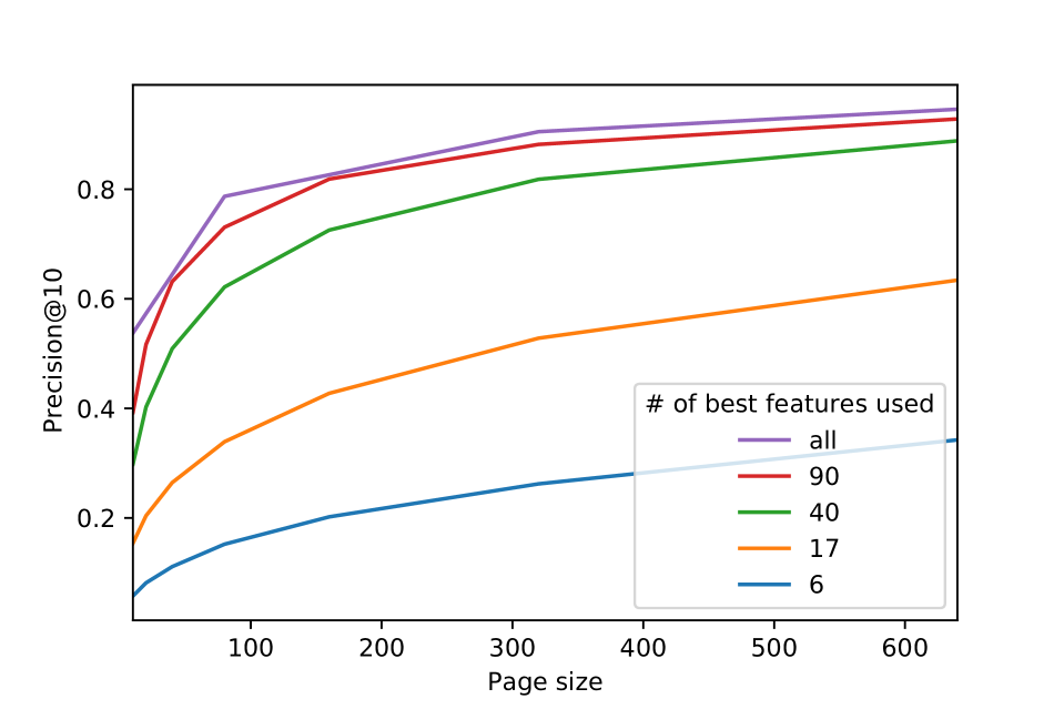
(b) Precision@10

Figure 1: The impact of the number of best features selected (with no trimming) and the page size (the number of search results retrieved from Elasticsearch) on Avg. diff. and Precision@10.

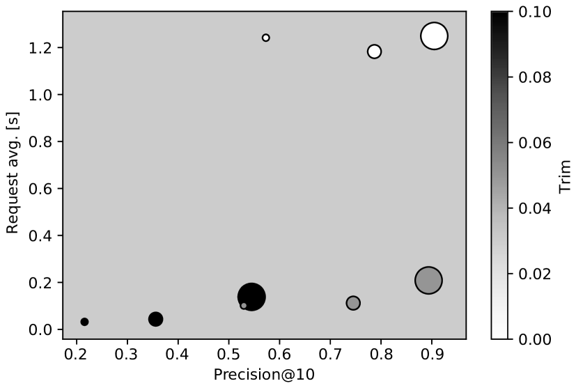
(a) Consecutive querying of 128 queries

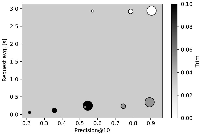
(b) Parallel querying in 4 parallel queues, 32 queries each (128 queries in total)

Figure 2: The impact of value filtering and the number of retrieved search results on the average request time. The x-axis shows the average precision, the y-axis the average request time. The size of the points indicates the number of retrieved results: large = Elasticsearch page size 320, medium = page size 80, small = 20. The color of the points indicates the trim thresholds: white = 0.00 (no filtering), gray = 0.05, black = 0.10.

Figure 1 illustrates the impact of feature value filtering and the number of retrieved search candidates from Elasticsearch (page size) on its accuracy. It can be seen that avg. diff. decreases logarithmically with the page size. The results improve all the way up to 640 search results (the maximum value we have tried), which is expected as this increases the size of the subset $E$ that is consequently ordered (re-ranked) in phase 2 with the precise but more costly exact algorithm. Increasing the size of $E$ increases the chance of the inclusion of relevant results.

The shape of the curve suggests that there would only be a slight improvement in accuracy, and this would be at the cost of a substantial drop in performance. The impact of including only a limited number of features with the highest absolute value (see Section 2.2.2), is rather low. This is an excellent result with regard to performance as it means we may effectively sparsify the query vector with very little impact on search quality. We observe little difference between no filtering (searching by all 400 encoded features) and trimming to only the 90 best query vector values. However, trimming to as low as 6 values results in a significant increase in avg. diff. See Figure 1(a).

Our methods scores above the MLT baseline in all of the followed metrics, even with aggressive high-pass filtering and with a small page size.

We expect that similar setup parameters will work similarly, at least for general multi-topic text datasets. Its behaviour for a dramatically different dataset, such as images instead of texts, or without normalized feature ranges, cannot be directly inferred and remains to be investigated in our future work. However, we expect our speed optimization methods to be applicable in some form, with the concrete parameters to be validated on the particular dataset and algorithmic setup.

4.2 Speed Evaluation

Selected results of our speed evaluation are summarized in Table 3. For clarity, we selected only the configurations using 400 LSA features and 48 Elasticsearch shards, as this setup turned out to provide the optimal performance on the Elasticsearch cluster and dataset we used according to the quality evaluation (see Section 4.1), where the same parameters were used.

Table 3: Results of speed evaluation using 400 LSA features, batches of 128 queries and 48 Elasticsearch shards. Column Parallel q. shows the number of parallel queries used together, Trim is the threshold for high-pass filtering of the features, Page is the number of vectors retrieved from Elasticsearch for each query (see Section 2.2.2), ES avg./std. is the average and standard deviation of the number of seconds per request Elasticsearch took, Request avg./std. is the average and deviation of the number of seconds per request including processing overheads, Total time is the total number of seconds for processing all requests, Vec. size avg./std. is the average/deviation of the number of values in query vectors that passed high-pass filtering.

Parallel q.	Trim	Page	ES avg. [s]	ES std. [s]	Request avg. [s]	Request std. [s]	Total time [s]	Vec. size avg.	Vec. size std.
01	0.00	020	1.1949	0.0737	01.2418	0.2864	160.760	400.0000	00.0000
01	0.00	080	1.1656	0.0710	01.1829	0.0713	153.246	400.0000	00.0000
01	0.00	320	1.2066	0.0893	01.2494	0.0894	161.783	400.0000	00.0000
01	0.05	020	0.0935	0.0202	00.1013	0.0204	014.521	093.5781	20.9268
01	0.05	080	0.0935	0.0214	00.1119	0.0228	015.898	091.5781	22.9822
01	0.05	320	0.1635	0.1014	00.2085	0.1032	028.360	087.2500	20.6908
01	0.10	020	0.0241	0.0057	00.0320	0.0057	005.574	019.3516	04.4222
01	0.10	080	0.0259	0.0059	00.0435	0.0061	007.107	019.0469	04.3027
01	0.10	320	0.0940	0.0966	00.1383	0.0971	019.357	018.0703	04.7863
04	0.00	020	2.9093	0.3943	02.9325	0.3989	094.750	400.0000	00.0000
04	0.00	080	2.8842	0.2968	02.9211	0.3004	094.548	400.0000	00.0000
04	0.00	320	2.8621	0.2897	02.9439	0.2938	095.290	400.0000	00.0000
04	0.05	020	0.1919	0.0491	00.2094	0.0531	007.212	089.3516	21.9351
04	0.05	080	0.2027	0.0525	00.2327	0.0563	007.948	093.2422	20.6166
04	0.05	320	0.2583	0.0983	00.3442	0.1025	011.538	086.3203	24.1855
04	0.10	020	0.0422	0.0080	00.0550	0.0078	002.253	018.8047	04.4547
04	0.10	080	0.0703	0.0708	00.1151	0.0884	004.174	019.5547	04.2625
04	0.10	320	0.1547	0.1093	00.2468	0.1161	008.411	017.8750	04.4459
16	0.00	020	11.5664	3.2998	11.6019	3.3018	094.480	400.0000	00.0000
16	0.00	080	11.5408	2.6209	11.6033	2.6262	094.535	400.0000	00.0000
16	0.00	320	11.5144	3.7843	11.7623	3.7645	095.112	400.0000	00.0000
16	0.05	020	0.7870	0.1988	00.8116	0.2020	006.896	088.4141	21.6681
16	0.05	080	0.7253	0.2309	00.8802	0.3051	007.463	087.9063	23.1528
16	0.05	320	0.8511	0.2350	01.0453	0.2491	009.332	089.9141	23.0604
16	0.10	020	0.1354	0.0182	00.1660	0.0169	001.625	018.4375	03.9484
16	0.10	080	0.1845	0.0859	00.2613	0.0891	002.400	018.7656	04.8404
16	0.10	320	0.4181	0.1442	00.6213	0.2065	005.416	018.0703	04.3807

The speed of the native Elasticsearch MLT search is summarized in Table 4. The speed is comparable to our method when high-pass filtering is involved.

Table 4: Results of speed evaluation using the native Elasticsearch More Like This (MLT) search (no parallel queries) using 48 shards. max_query_terms is the maximum number of query terms per query that were selected by Elasticsearch. ES avg./std. is the average and standard deviation of the number of seconds per request Elasticsearch took.

System	max_query_terms	ES avg. [s]	ES std. [s]
MLT	017	0.0468	0.0233
MLT	025	0.0595	0.0270
MLT	040	0.0745	0.0322
MLT	090	0.1090	0.0490
MLT	400	0.1458	0.0978

Figure 2 displays the impact of value filtering and the number of retrieved search results on the average request time. Comparing consecutive queries (Figure 2(a)) with four parallel queries on the same Elasticsearch cluster configuration (Figure 2(b)) shows that at the expense of doubling the response time, we are able to answer four requests in parallel.

The best results in Figure 2 are located in the bottom right corner where the precision is high and the response time is low. For our dataset and algorithm (LSA with 400 features), the best overall results are represented by the largest gray dots, i.e. retrieving 320 vectors from Elasticsearch while filtering the query vector to roughly 90 values via trimming with a threshold of 0.05.

To achieve the optimal results, we suggest retrieving as large a set of candidates (Elasticsearch page size, $E$) as the response-time constraints allow, as the page size seems to have significantly lower influence on the response time compared to trimming, while having a significant positive effect on accuracy.

Our experiments were done on the Wikipedia dataset. Wikipedia is a multi-topic dataset – articles are on a wide variety of different topics using different keywords (names of people, places and things, etc) and notation (text only articles, articles on mathematics using formulae, articles on chemistry using different formulae, etc) are included. This provides enough room for the machine learning algorithms to build features that reflect these unique markers of particular topics and makes particular features significantly irrelevant for particular documents in the dataset.

For general multi-topic text datasets, we recommend trimming features values by their absolute value below 5% of the maximum (i.e. between $-0.05$ and 0.05 in our experiments). Trimming more feature tokens decreases the precision with almost no influence on the response times, while keeping more feature tokens in the index has almost no positive effect on the precision but slows down the search significantly.

5 Conclusions

In this paper we have demonstrated a novel method for the conversion of semantic vectors into a set of string ‘feature tokens’ that can be subsequently indexed in a standard inverted-index-based fulltext search engine, such as Elasticsearch.

Two techniques of feature tokens filtering were demonstrated to further significantly speed up the search process, with an acceptably low impact on the quality of the results.

Using Elasticsearch MLT on document texts as a baseline, our method performs better than the baseline on all the followed metrics. With sufficient query vector feature reduction, our method is faster than MLT. With moderate query vector feature reduction, we can achieve excellent approximation of the gold standard while being only marginally slower than the MLT.

An important conclusion from our experiments is that the search speed can be improved even with filtering the query vectors alone and without the need to trim index vectors. A pleasant practical consequence of this finding is that a vector search engine based on our proposed scheme could allow the users to define the filtering parameters dynamically, at search time rather than at indexing time. In this way, we let the users choose the approximation trade-off between the search speed and accuracy, i.e. use weaker filtering parameters for searches where accuracy is critical, and more aggressive filtering where speed is critical.

In our future work we will focus on the validation of our techniques on different types of data (such as images or audio data) and different text representations (such as doc2vec) in specific domains (such as question answering).

Acknowledgments

Funding by TA ČR Omega grant TD03000295 is gratefully acknowledged.

References

- Blei et al. (2003) David M. Blei, Andrew Y. Ng, Michael I. Jordan, and John Lafferty. 2003. Latent Dirichlet Allocation. Journal of Machine Learning Research 3:993–1022. http://dl.acm.org/citation.cfm?id=944919.944937.
- Boytsov (2017) Leonid Boytsov. 2017. Efficient and Accurate Non-Metric -NN Search with Applications to Text Matching. Thesis proposal, School of Computer Science, Carnegie Mellon University. http://boytsov.info/pubs/proposal_boytsov.pdf.
- Deerwester et al. (1990) Scott Deerwester, Susan T. Dumais, George W. Furnas, Thomas K. Landauer, and Richard Harshman. 1990. Indexing by Latent Semantic Analysis. Journal of the American Society for Information Science 41(6):391–407.
- Digout et al. (2004) Christian Digout, Mario A. Nascimento, and Alexandru Coman. 2004. Similarity search and dimensionality reduction: Not all dimensions are equally useful. In YoonJoon Lee, Jianzhong Li, Kyu-Young Whang, and Doheon Lee, editors, Proc. of Database Systems for Advanced Applications: 9th Int. Conf., DASFAA 2004, Jeju Island, Korea, March 17–19, 2003. Springer, pages 831–842. https://doi.org/10.1007/978-3-540-24571-1_73.
- Gionis et al. (1999) Aristides Gionis, Piotr Indyk, and Rajeev Motwani. 1999. Similarity search in high dimensions via hashing. In VLDB ’99, Proceedings of 25th International Conference on Very Large Data Bases, September 7–10, 1999, Edinburgh, Scotland, UK. pages 518–529. http://www.vldb.org/conf/1999/P49.pdf.
- Gormley and Tong (2015) Clinton Gormley and Zachary Tong. 2015. Elasticsearch: The Definitive Guide. O’Reilly Media, Inc., 1st edition.
- Le and Mikolov (2014) Quoc V. Le and Tomas Mikolov. 2014. Distributed representations of sentences and documents. CoRR abs/1405.4053. http://arxiv.org/abs/1405.4053.
- Manning et al. (2008) Christopher D. Manning, Prabhakar Raghavan, and Hinrich Schütze. 2008. Introduction to Information Retrieval. Cambridge University Press, New York, NY, USA.
- Mikolov et al. (2013) Tomas Mikolov, Ilya Sutskever, Kai Chen, Greg S Corrado, and Jeff Dean. 2013. Distributed representations of words and phrases and their compositionality. In Advances in Neural Information Processing Systems. pages 3111–3119.
- Rygl et al. (2016) Jan Rygl, Petr Sojka, Michal Růžička, and Radim Řehůřek. 2016. ScaleText: The Design of a Scalable, Adaptable and User-Friendly Document System for Similarity Searches: Digging for Nuggets of Wisdom in Text. In Aleš Horák, Pavel Rychlý, and Adam Rambousek, editors, Proceedings of the Tenth Workshop on Recent Advances in Slavonic Natural Language Processing, RASLAN 2016. Tribun EU, Brno, pages 79–87. https://nlp.fi.muni.cz/raslan/2016/paper08-Rygl_Sojka_etal.pdf.
- Salton and Buckley (1988) Gerard Salton and Chris Buckley. 1988. Term-weighting approaches in automatic text retrieval. Information Processing and Management 24:513–523.
- Salton et al. (1975) Gerard Salton, Anita Wong, and Chung-Shu Yang. 1975. A vector space model for automatic indexing. Communications of the ACM 18(11):613–620. https://doi.org/10.1145/361219.361220.
- Weber and Böhm (2000) Roger Weber and Klemens Böhm. 2000. Trading quality for time with nearest-neighbor search. In Carlo Zaniolo, Peter C. Lockemann, Marc H. Scholl, and Torsten Grust, editors, Proc. of Advances in Database Technology — EDBT 2000: 7th Int. Conf. on Extending Database Technology Konstanz, Germany, March 27–31, 2000. Springer, pages 21–35. https://doi.org/10.1007/3-540-46439-5_2.
- Weber et al. (1998) Roger Weber, Hans-Jörg Schek, and Stephen Blott. 1998. A quantitative analysis and performance study for similarity-search methods in high-dimensional spaces. In Proc. of the 24rd International Conference on Very Large Data Bases. Morgan Kaufmann Publishers Inc., San Francisco, CA, USA, VLDB ’98, pages 194–205. http://dl.acm.org/citation.cfm?id=645924.671192.
- Zezula et al. (2006) Pavel Zezula, Giuseppe Amato, Vlastislav Dohnal, and Michal Batko. 2006. Similarity Search: The Metric Space Approach, volume 32 of Advances in Database Systems. Springer.