Generalized $\mathbb{Z}_{2}\times\mathbb{Z}_{2}$ in Scaling neutrino Majorana mass matrix and baryogenesis via flavored leptogenesis

Abstract

We investigate the consequences of a generalized $\mathbb{Z}_{2}\times\mathbb{Z}_{2}$ symmetry on a scaling neutrino Majorana mass matrix. It enables us to determine definite analytical relations between the mixing angles $\theta_{12}$ and $\theta_{13}$, maximal CP violation for the Dirac type and vanishing for the Majorana type. Beside the other testable predictions on the low energy neutrino parameters such as $\beta\beta_{0\nu}$ decay matrix element $|M_{ee}|$ and the light neutrino masses $m_{1,2,3}$, the model also has intriguing consequences from the perspective of leptogenesis. With the assumption that the required CP violation for leptogenesis is created by the decay of lightest ($N_{1}$) of the heavy Majorana neutrinos, only $\tau$-flavored leptogenesis scenario is found to be allowed in this model. For a normal (inverted) ordering of light neutrino masses, $\theta_{23}$ is found be less (greater) than its maximal value, for the final baryon asymmetry $Y_{B}$ to be in the observed range. Besides, an upper and a lower bound on the mass of $N_{1}$ have also been estimated. Effect of the heavier neutrinos $N_{2,3}$ on final $Y_{B}$ has been worked out subsequently. The predictions of this model will be tested in the experiments such as nEXO, LEGEND, GERDA-II, T2K, NO$\nu$A, DUNE etc.

1 Introduction

The neutrino oscillation data, adhering to the bound on the sum of the three electroweak neutrino masses and the results of $\beta\beta_{0\nu}$ decay experiments severely constrain the textures of light neutrino mass matrix. Admissible textures of the mass matrix satisfying the above experimental constraints thus can be tested in future through their predictions regarding the yet unresolved issues such as the hierarchy of neutrino masses, octant determination of $\theta_{23}$, and particularly, CP violation in the leptonic sector which might have implication on the matter-antimatter asymmetry of the universe. Besides, if neutrino is a Majorana particle, the prediction of Majorana phases will also serve as an added ingredient to discriminate different models. From the symmetry point of view thus it is a challenging task to integrate theoretical considerations involving different symmetry/ansatz in addition to the Standard Model (SM).

Recently, the idea of residual symmetry[res, dicus] has attracted much attention to explore the flavor structure of light neutrino mass matrix. In this approach, the neutrino mass matrix is attributed some residual or remnant symmetry of a horizontal flavor group. It can be shown that the Majorana type nondegenerate light neutrinos lead to an invariance of the effective light neutrino mass matrix under a $\mathbb{Z}_{2}\times\mathbb{Z}_{2}$ symmetry accompanied with a charged lepton mass matrix that enjoys a $\mathbb{Z}_{n}$ invariance with $n>2$ [res]. Now it is a challenging task to find out larger symmetry groups which embed these remnant symmetries. Nevertheless, for some predictive residual symmetries, a list of horizontal symmetry groups has been addressed by Lam[res]. In addtion, viability of Coxeter groups as horizontal symmetries in the leptonic sector has been studied recently in Ref.[pal]. Although some of the groups that belong to the Coxeter class have been analyzed in literature (e.g., $S_{4}$), still there are scopes for a detail study of these groups in the leptonic sector, specifically in the context of grand unified model such as SO(10) that contains Coxeter group as a built-in symmetry[Lam:2014kga]. Furthermore, to constrain the CP violating phases, a $\mu\tau$-interchange symmetry has been used to implement a nonstandard CP transformation in Ref.[CP]. Inspired by these well accepted road maps that redirect physicists towards the quest for an ultimate elusive model, in the present work we study the effect of a generalized $\mathbb{Z}_{2}\times\mathbb{Z}_{2}$[joshi] that replicates scaling ansatz[scl, scl2] in conjunction with a nonstandard CP transformation on light neutrino Majorana mass matrix.

We first consider a general neutrino mass matrix $M_{\nu}^{0}$ with scaling ansatz invariance as an effective low energy symmetry and following residual symmetry approach, interpret the latter as a residual $\mathbb{Z}_{2}\times\mathbb{Z}_{2}$ symmetry. Due to the outcome of a vanishing reactor angle $\theta_{13}$ (which is excluded by experiment at more than $5.2\sigma$[th13]), we further use these $\mathbb{Z}_{2}$ generators to implement CP transformations. Thus instead of an ordinary $\mathbb{Z}_{2}\times\mathbb{Z}_{2}$ symmetry, we now demand a generalized $\mathbb{Z}_{2}\times\mathbb{Z}_{2}$ as an effective residual symmetry that extend the scaling ansatz to its complex counterpart. In this case, having a more complicated scaling relationship between its elements, the resultant mass matrices (depending upon the ways of implementation of the symmetry, actually there are two light neutrino mass matrices) are further reconstructed through the type-I seesaw mechanism which incorporates three right chiral singlet neutrino fields $N_{iR}$ $(i=1,2,3)$ in addition to the regular SM field contents. Although it is nontrivial to combine a flavor and a CP symmetry[Feru1, Holthausen:2012dk, Chen:2014tpa], a consistent definition for both of them is possible when they satisfy certain condition–usually known as the consistency condition[Holthausen:2012dk, Chen:2014tpa, King:2017guk]. However, at low energy this combined symmetry should be broken to different symmetries in the neutrino and the charged lepton sector, since it is known that at least a common residual CP symmetry in both the sector would imply a vanishing CP violation[Feru1, Holthausen:2012dk, King:2017guk]. Although here we do not focus on the explicit construction of the high energy flavor group, throughout the analysis we assume a diagonal and nondegenerate charged lepton mass matrix which is protected by a residual symmetry $G_{\ell}$ after the spontaneous breaking of the combination of CP and flavor symmetry at high energy[Feru1, King:2017guk, Ding:2013hpa]. Depending upon the breaking pattern, there may also be a trivial or a nontrivial CP symmetry in the charged lepton sector[Li:2013jya]. However, as pointed out, the final residual CP symmetries in both the sectors should be different. One can also construct a minimal high energy group from a bottom-up approach knowing the symmetry in the neutrino sector and then finding the symmetry in the charged lepton sector with the automorphism condition as described in Ref [Feru2, Nishi:2016wki].

Finally, using the oscillation constraints, tantalizing predictions on the low energy parameters such as neutrino masses, neutrinoless double beta decay, CP violating phases are obtained. Due to the presence of three massive right handed (RH) neutrinos, baryogenesis via leptogenesis scenario is also explored. Interesting conclusions such as octant sensitivity of the atmospheric mixing angle $\theta_{23}$, preconditioned by the observed range of the final baryon asymmetry $Y_{B}$ and nonoccurrence of unflavored leptogenesis are also drawn.

The paper is organized as follows. Section 2 contains a brief discussion on residual symmetry and scaling ansatz with a possible modification to the ansatz by extending the former with a nonstandard CP transformation. In section 3 we discuss a type-I seesaw extension of the analysis made in the previous section. Section 4 contains a discussion about baryogenesis via leptogenesis scenario related to the present model. In section 5 we present detail results of the numerical analysis. A discussion on the sensitivity of the heavier neutrinos to the obtained results for the final $Y_{B}$ is presented in section LABEL:s6. Section LABEL:s7 concludes the entire discussion with some promising remarks.

2 Modification to scaling neutrino mass matrix with generalized $\mathbb{Z}_{2}\times\mathbb{Z}_{2}$

Before going to an explicit details of our work, let us first discuss the residual $\mathbb{Z}_{2}\times\mathbb{Z}_{2}$ symmetry proposed in Ref.[res]. A Majorana neutrino mass matrix $M_{\nu}$ enjoys a $\mathbb{Z}_{2}\times\mathbb{Z}_{2}$ flavor symmetry which can be envisaged as a remnant symmetry of some horizontal flavor group. These horizontal symmetry groups are preferably finite groups since in that case the theory has a more predictive power due to the discrete number of choices for the residual symmetries $G_{i}$[res]. A bottom up as well as a top down approach for a viable horizontal group has been studied in the first one of Ref.[res]. There are plenty of horizontal groups that have been explored in the literature, among them finite groups such as $O_{h}$[Feru3], $\mathbb{Z}_{m}$[Koide:2002cj], $\mathbb{Z}_{m}\times\mathbb{Z}_{n}$[Ghosal:2002mz], $D_{n}$[Grimus:2004rj], $S_{4}$[Pakvasa:1978tx], $A_{4}$[Ma:2001dn], $\Delta(27)$[Branco:1983tn] and infinite groups such as $SO(3)$ and $SU(3)$[King:2003rf] have drawn much attention.
A linear transformation of the neutrino fields $\nu_{L\alpha}\to G_{\alpha\beta}\nu_{L\beta}$ leads to an invariance of an effective neutrino Majorana mass term

$$-\mathcal{L}^{\nu}_{mass}=\frac{1}{2}\bar{\nu}^{C}_{L\alpha}(M_{\nu})_{\alpha\beta}\nu_{L\beta}+{\rm h.c.},$$ (2.1)

if the mass matrix $M_{\nu}$ satisfies the invariance equation

$$G^{T}M_{\nu}G=M_{\nu}.$$ (2.2)

Here $G$ is a $3\times 3$ unitary matrix in flavor basis. It has been shown in Ref.[res] that if an unitary matrix $U$ diagonalizes $M_{\nu}$ then the matrix $U^{\prime}=GU$ also does so where $U^{\prime}$ satisfies the condition

$$GU=Ud~{}~{}{\rm with}~{}~{}d_{lm}=\pm\delta_{lm}.$$ (2.3)

Among the eight possible choices for $d$, only two of them can be shown to be independent on account of the relation $d_{a}d_{b}=d_{b}d_{a}=d_{c}$, which implies $G_{a}G_{b}=G_{b}G_{a}=G_{c}$ with $a\neq b\neq c$. These two independent $G$ matrices define a $\mathbb{Z}_{2}\times\mathbb{Z}_{2}$ symmetry since $d^{2}=G^{2}=I$ as dictated by Eq.(2.3). Thus given a mass matrix $M_{\nu}$, one can obtain $U$ consistent with the symmetries of $M_{\nu}$. From which $G_{a}$’s can be obtained as

$$G_{a}=Ud_{a}U^{\dagger}$$ (2.4)

with $a=1,2,3$. Since $G^{2}=I$ implies ${\rm det}~{}G=\pm 1$, one can choose the independent $d$ matrices corresponding to any value for the determinant of the $G$ matrices. Here without loss of generality, we choose to proceed with ${\rm det}~{}G=+1$ that corresponds to the structure of $d$ matrices as $d_{1}={\rm diag}~{}(1,-1,-1)$, $d_{2}={\rm diag}~{}(-1,1,-1)$ and $d_{3}=d_{1}d_{2}$.

Basically for an arbitrary mixing matrix $U$, one can construct a unique $G$, however the reverse is not true due to the degeneracies in the eigenvalues of $d_{a}$ matrices. From this point, the implementation of the residual symmetry to the neutrino mass matrix takes different paths. Given a leading order mixing matrix, e.g. $U^{\mu\tau}$, construction of $G$ matrices are unique, then for a particular $G$ matrix, one might or might not have $U^{\mu\tau}$. Papers such as [dicus] discuss scenarios like soft breaking of one of the two residual symmetries such that presence of the other with its degenerate eigenvalues enhances the degrees of choice of the mixing matrix in accordance with the phenomenological requirement. On the other hand, in Ref.[CP, joshi, val], as a more predictive scenario, invariance of the neutrino mass matrix under an extended $\mu\tau$ symmetry (${\rm CP}^{\mu\tau}$ or CP transformation with the $\mu\tau$-symmetry) has been considered. Both the schemes have their own uniqueness in terms of the predictions on the low energy neutrino parameters. However, in this work, we follow the second approach due to its robust predictions on CP violating phases which are related to the matter antimatter asymmetry of the universe[planck].

We interpret the Strong Scaling Ansatz (SSA) proposed in Ref.[scl], as a residual $\mathbb{Z}_{2}\times\mathbb{Z}_{2}$ symmetry. Since SSA leads to a vanishing $\theta_{13}$, a possible modification to this has been made by generalizing the two independent ordinary $\mathbb{Z}_{2}$ invariance to their complex counterpart, i.e., two independent $\mathbb{Z}_{2}^{\rm CP}$ invariance. Thus the SSA has been extended to its complex version by means of a generalized $\mathbb{Z}_{2}\times\mathbb{Z}_{2}$ symmetry (see Ref.[joshi] for another such extension in case of TBM mixing). Let’s discuss now the exact methodology of our analysis:

We consider a column wise scaling relations in the elements of $M^{0}_{\nu}$ in flavor space as

$$\frac{(M_{\nu}^{0})_{e\mu}}{(-M_{\nu}^{0})_{e\tau}}=\frac{(M_{\nu}^{0})_{\mu\mu}}{(-M_{\nu}^{0})_{\mu\tau}}=\frac{(M_{\nu}^{0})_{\tau\mu}}{(-M_{\nu}^{0})_{\tau\tau}}=k,$$ (2.5)

where $k$ is a real and positive dimensionless scaling factor. The superscript ‘0’ on $M_{\nu}$ symbolizes SSA as a leading order matrix in this analysis. Now the structure for $M_{\nu}^{0}$ dictated by the ansatz of Eq.(2.5) comes out as

$$M_{\nu}^{0}=\begin{pmatrix}P&-Qk&Q\\ -Qk&Rk^{2}&-Rk\\ Q&-Rk&R\end{pmatrix}.$$ (2.6)

Here $P,Q,R$ are a priori unknown, complex mass dimensional quantities. The minus sign in Eq.(2.5) has been considered to be in conformity with the PDG convention[pdg]. The matrix in Eq.(2.6) is diagonalized by a unitary matrix $U^{0}$ having a form

$$U^{0}=\begin{pmatrix}c_{12}^{0}&s_{12}^{0}e^{i\alpha}&0\\ -\frac{ks_{12}^{0}}{\sqrt{1+k^{2}}}&\frac{kc_{12}^{0}}{\sqrt{1+k^{2}}}e^{i\alpha/2}&\frac{1}{\sqrt{1+k^{2}}}e^{i\beta/2}\\ \frac{s_{12}^{0}}{\sqrt{1+k^{2}}}&-\frac{c_{12}^{0}}{\sqrt{1+k^{2}}}e^{i\alpha/2}&\frac{k}{\sqrt{1+k^{2}}}e^{i\beta/2}\\ \end{pmatrix},$$ (2.7)

where $c_{12}^{0}=\cos\theta_{12}^{0}$, $s_{12}^{0}=\sin\theta_{12}^{0}$ which are calculated in terms of the parameters of $M_{\nu}^{0}$, and $\alpha,\beta$ represents the Majorana phases. SSA predicts a vanishing $\theta_{13}$ (hence no measurable leptonic Dirac CP-violation) as one can see from Eq.(2.7) and an inverted neutrino mass ordering (i.e., $m_{2,1}>m_{3}$), with $m_{3}=0$. As previously mentioned, one needs to modify the ansatz to generate a non-zero $\theta_{13}$. Now using the paradigm of residual symmetry as described in the earlier part of this section, one can calculate the $G_{a}$ matrices using the relation

$$G_{a}^{(k)}=U^{0}d_{a}U^{0\dagger}$$ (2.8)

with $G_{a}^{(k)}$ as the $\mathbb{Z}_{2}$ generators for a scaling ansatz invariant $M_{\nu}$. Similar to Eq.(2.2), $M_{\nu}^{0}$ will then satisfy the invariance equation

$$\Big{(}G_{a}^{(k)}\Big{)}^{T}M^{0}_{\nu}G_{a}^{(k)}=M^{0}_{\nu}.$$ (2.9)

Now using Eq.(2.8) we calculate the corresponding $G_{a}^{(k)}$ ($a=1,2,3$) matrices and present them as

$$G_{1}^{(k)}=\begin{pmatrix}\cos 2\theta^{0}_{12}&-k(1+k^{2})^{-1/2}\sin 2\theta^{0}_{12}&-(1+k^{2})^{-1/2}\sin 2\theta^{0}_{12}\\ -k(1+k^{2})^{-1/2}\sin 2\theta^{0}_{12}&-(1+k^{2})^{-1}(k^{2}\cos 2\theta^{0}_{12}+1)&-k(1+k^{2})^{-1}(1-\cos 2\theta^{0}_{12})\\ -(1+k^{2})^{-1/2}\sin 2\theta^{0}_{12}&-k(1+k^{2})^{-1}(1-\cos 2\theta^{0}_{12})&-(1+k^{2})^{-1}(k^{2}+\cos 2\theta^{0}_{12})\end{pmatrix},$$ (2.10)

$$G_{2}^{(k)}=\begin{pmatrix}-\cos 2\theta^{0}_{12}&k(1+k^{2})^{-1/2}\sin 2\theta^{0}_{12}&-(1+k^{2})^{-1/2}\sin 2\theta^{0}_{12}\\ k(1+k^{2})^{-1/2}\sin 2\theta^{0}_{12}&(1+k^{2})^{-1}(k^{2}\cos 2\theta^{0}_{12}-1)&-k(1+k^{2})^{-1}(1+\cos 2\theta^{0}_{12})\\ -(1+k^{2})^{-1/2}\sin 2\theta^{0}_{12}&-k(1+k^{2})^{-1}(1+\cos 2\theta^{0}_{12})&-(1+k^{2})^{-1}(k^{2}-\cos 2\theta^{0}_{12})\end{pmatrix},$$ (2.11)

$$G^{(k)}_{3}=\begin{pmatrix}-1&0&0\\ 0&(1-k^{2})(1+k^{2})^{-1}&2k(1+k^{2})^{-1}\\ 0&2k(1+k^{2})^{-1}&-(1-k^{2})(1+k^{2})^{-1}\end{pmatrix}.$$ (2.12)

Note that all the $G^{(k)}_{a}$ matrices are symmetric by construction. Now to modify SSA, we generalize this $\mathbb{Z}_{2}\times\mathbb{Z}_{2}$ by implementing CP transformations on the neutrino fields[CPt] with the $\mathbb{Z}_{2}$ generators ($G_{a}^{(k)}={G_{a}^{(k)}}^{T}$) as

$$\nu_{L\alpha}\to i(G_{a}^{(k)})_{\alpha\beta}\gamma^{0}\nu^{C}_{L\beta}.$$ (2.13)

This extends the real horizontal invariance of $M_{\nu}^{0}$ in Eq.(2.9) to its complex counterpart, i.e.

$$\Big{(}G_{a}^{(k)}\Big{)}^{T}M_{\nu}G_{a}^{(k)}=M_{\nu}^{*}.$$ (2.14)

Therefore the SSA, elucidated as a $\mathbb{Z}_{2}\times\mathbb{Z}_{2}$ symmetry, has now been modified to an extended SSA, interpreted as a complex $\mathbb{Z}_{2}\times\mathbb{Z}_{2}$ symmetry which is some time also referred as a generalized $\mathbb{Z}_{2}\times\mathbb{Z}_{2}$ symmetry of $M_{\nu}$[joshi]. In the next subsections we show that there are only two ways in which such a complex extension can be done.

2.1 Case I: Complex extension of $G_{2,3}^{(k)}$ Invariance

The complex invariance relations of $M_{\nu}$ related to $G_{2,3}^{(k)}$ is now written as

$$\Big{(}G_{2,3}^{(k)}\Big{)}^{T}M_{\nu}G_{2,3}^{(k)}=M_{\nu}^{*},$$ (2.15)

which in turn implies

$$\Big{(}G_{1}^{(k)}\Big{)}^{T}M_{\nu}G_{1}^{(k)}=M_{\nu}$$ (2.16)

owing to the closure property of the $G^{(k)}_{a}$ ($a=1,2,3$) matrices.

Eq.(2.15) leads to a most general Majorana neutrino mass matrix of the form

$$M_{\nu}^{MS1}=\begin{pmatrix}p&-q_{1}k+i\frac{q_{2}}{k}&q_{1}+iq_{2}\\ -q_{1}k+i\frac{q_{2}}{k}&r-\frac{s(k^{2}-1)}{k}+i\frac{2q_{2}\kappa_{+}}{\sqrt{1+k^{2}}}&s+i\frac{q_{2}\kappa_{+}(k^{2}-1)}{k\sqrt{1+k^{2}}}\\ q_{1}+iq_{2}&s+i\frac{q_{2}\kappa_{+}(k^{2}-1)}{k\sqrt{1+k^{2}}}&r-i\frac{2q_{2}\kappa_{+}}{\sqrt{1+k^{2}}}\end{pmatrix}$$ (2.17)

with

$$r=(sk+p)-q_{1}\sqrt{1+k^{2}}(\kappa_{+}-\frac{1}{\kappa_{+}}),$$ (2.18)

$$\kappa_{+}=(\cot 2\theta_{12}^{0}+{\rm cosec}2\theta_{12}^{0}).$$ (2.19)

Here $p$, $q_{1,2}$, $r$ and $s$ are real, mass dimentional quantities and the superscript ‘$MS$’ stands for ‘Modified Scaling’. It has already been shown in Ref.[Rome] that $(G_{3}^{(k)})^{T}M_{\nu}G_{3}^{(k)}=M_{\nu}^{*}$ leads to the results

$$\tan\theta_{23}=k^{-1},$$ (2.20)

$$\sin\alpha=\sin\beta=\cos\delta=0.$$ (2.21)

Now in the present case, the overall real $G_{1}^{(k)}$ (cf. Eq.(2.16)) invariance of $M_{\nu}$ fixes the first column of $U_{PMNS}$ to the first column of $U^{0}$. Therefore, one gets the relation between the solar and the reactor mixing angle as

$$|\cos\theta_{12}\cos\theta_{13}|=\cos\theta^{0}_{12}\Rightarrow\sin^{2}\theta_{12}=1-\cos^{2}\theta^{0}_{12}(1+\tan^{2}\theta_{13}).$$ (2.22)

2.2 Case II: Complex extension of $G_{1,3}^{(k)}$ Invariance

In this case, the complex invariance relations of $M_{\nu}$ due to $G_{1,3}^{(k)}$ can be written as

$$\Big{(}G_{1,3}^{(k)}\Big{)}^{T}M_{\nu}G_{1,3}^{(k)}=M_{\nu}^{*},$$ (2.23)

which leads to

$$\Big{(}G_{2}^{(k)}\Big{)}^{T}M_{\nu}G_{2}^{(k)}=M_{\nu}.$$ (2.24)

Eq.(2.23) leads to the mass matrix $M_{\nu}^{MS2}$ having a form same as $M_{\nu}^{MS1}$ as given in Eq.(2.17) where $\kappa_{+}$ is replaced with $\kappa_{-}=-1/\kappa_{+}$. Similar to the previous case, a complex invariance due to $G_{3}^{(k)}$ leads to the predictions

$$\tan\theta_{23}=k^{-1},$$ (2.25)

$$\sin\alpha=\sin\beta=\cos\delta=0.$$ (2.26)

Now the overall real $G_{2}^{(k)}$ (cf. Eq.(2.24)) invariance of $M_{\nu}$ fixes the second column of $U_{PMNS}$ to the second column of $U^{0}$ which gives rise to a relation between the solar and the reactor mixing angle as

$$|\sin\theta_{12}\cos\theta_{13}|=\sin\theta^{0}_{12}\Rightarrow\sin^{2}\theta_{12}=\sin^{2}\theta^{0}_{12}(1+\tan^{2}\theta_{13}).$$ (2.27)

Similar to the previous cases, complex invariance due to $G_{1,2}^{(k)}$ leads to an overall real invariance due to $G_{3}^{(k)}$ which leads to a vanishing $\theta_{13}$. Thus this is a case of least interest. For both the viable cases, we determine three CP phases ($\cos\delta=0,\alpha,\beta=0$ or $\pi$). Thus there are 6 real free parameters $p,q_{1,2},s,k$ and $\kappa_{+}$ (or $\theta^{0}_{12}$) (cf. Eq.(2.17)) in both the mass matrices. However, one can trivially track the parameters $k$ and $\theta_{12}^{0}$ on account of the relations in (2.20) or (2.25) and (2.22) or (2.27). Thus the other four parameters account for one mixing angle and three neutrino masses. However, to fix the absolute neutrino mass scale, we additionally use some constraints from baryogenesis as discussed in the numerical section.

We note that the prediction of the CP phases in the extended SSA scheme are identical to the case of ${\rm CP}^{\mu\tau}$[CP]. Therefore the question arises how one might distinguish the ${\rm CP}^{\mu\tau}$ and the extended SSA experimentally? First of all, both the Strong Scaling Ansatz (SSA) and the $\mu\tau$ symmetry lead to $\theta_{13}=0$ at the leading order and therefore, has to be abandoned. However, one can in principle differentiate SSA from the $\mu\tau$ reflection symmetry via their predictions of atmospheric mixing angle $\theta_{23}$. The former in general predicts a nonmaximal $\theta_{23}$ (for $k\neq 1$) given by $\theta_{23}=\tan^{-1}(k^{-1})$ while a maximal value ($\theta_{23}=\pi/4$) is predicted by the latter.

Furthermore, in the extended scheme, besides the similar predictions for the CP phases an arbitrary nonvanishing value of the reactor mixing angle $\theta_{13}$ is predicted in both the cases (extended SSA and ${\rm CP}^{\mu\tau}$). However, the prediction on the $\theta_{23}$ is different for each case. Interestingly, even after the extension, the value of $\theta_{23}$ survives for both the cases i.e., $\theta_{23}=\tan^{-1}(k^{-1})$ for the SSA as well as extended SSA and $\theta_{23}=\pi/4$ for $\mu\tau$ symmetry and its extended version (${\rm CP}^{\mu\tau}$). If experiments find a nonmaximal $\theta_{23}$ at a significant confidence level (recently there is a hint from NO$\nu$A regarding the nonmaximality of $\theta_{23}$ at 2.6 $\sigma$ CL[Adamson:2017qqn]) then the ${\rm CP}^{\mu\tau}$ symmetry will be ruled out while our proposal of an extended SSA (that predicts a nonmaximal $\theta_{23}$ in general) will continue to survive.

Before proceeding further we should comment on the fulfillment of the consistency conditions[Holthausen:2012dk, Chen:2014tpa, King:2017guk] as mentioned in the introduction. Here we have discussed two cases. In the first one $G_{2,3}^{(k)}$ are the CP symmetries which further result in a $G_{1}^{(k)}$ invariance of the mass term while in the second case, the CP generators $G_{1,3}^{(k)}$ lead to an invariance of the mass term due to the $G_{2}^{(k)}$. Now the consistency condition in case of a $\mathbb{Z}_{2}$ group implies[King:2017guk]

$$X_{r}\rho_{r}^{*}(g)X_{r}^{-1}=\rho_{r}(g),$$ (2.28)

where $X_{r}$ is a unitary matrix representing CP symmetry which acts on a generic multiplet $\varphi$ as

$$X_{r}\varphi(x)\xrightarrow{\text{CP}}X_{r}\varphi(x^{\prime})$$ (2.29)

with $x^{\prime}=(t,-{\bf x})$ and $\rho_{r}(g)$ is a representation for the element $g$ of the flavor group in an irreducible representation ${\bf r}$. In our analysis, $G_{i}^{(k)}$’s are real, and hence, the condition in Eq.(2.28) turns out to be

$$G_{2,3}^{(k)}G_{1}^{(k)}(G_{2,3}^{(k)})^{-1}=G_{1}^{(k)}~{}~{}~{}{\rm for}~{}~{}{\rm Case~{}I};$$

$$G_{1,3}^{(k)}G_{2}^{(k)}(G_{1,3}^{(k)})^{-1}=G_{2}^{(k)}~{}~{}~{}{\rm for}~{}~{}{\rm Case~{}II}.$$ (2.30)

Since $\Big{(}{G_{i}^{(k)}}\Big{)}^{2}=1$, $\Big{(}{G_{i}^{(k)}}\Big{)}^{-1}=G_{i}^{(k)}$ and each $G_{i}^{(k)}$ commutes with each other, the consistency condition is trivially satisfied for both the cases. However the main challenge is to ensure that such conditions are fulfilled for the larger (embedding) symmetries[Feru1, Holthausen:2012dk, Chen:2014tpa] which we do not explore here in this work.

Resolving the shortcomings of SSA, both the viable modified SSA matrices, referred as $M_{\nu}^{MS1}$ and $M_{\nu}^{MS2}$, possess intriguing phenomenology. This has been discussed in section 5 on numerical analysis. For the time being let’s focus on the implementation of the symmetry in a more specific way. So far we have discussed a possible complex extension for a general $M_{\nu}$, not so about the origin of the neutrino masses. This would be interesting to see the effects of generalized $\mathbb{Z}_{2}\times\mathbb{Z}_{2}$ on a particular mechanism that generates the light neutrino masses. Obviously, the choice depends upon the phenomenological interest. Here we choose the type-I seesaw mechanism and investigate possible consequences of the generalized $\mathbb{Z}_{2}\times\mathbb{Z}_{2}$ to explore the phenomena of baryogenesis via leptogenesis. A detailed discussion about these has been presented in the next two sections. First, we show the reconstruction of the effective modified SSA matrices through type-I seesaw mechanism with proper implementation of the symmetry on the constituent matrices ($m_{D}$ and $M_{R}$). Then we discuss some aspects of baryogenesis via leptogenesis related to this scheme.

3 Reconstruction of modified scaling matrices with type-I seesaw

For the realization of generalized $\mathbb{Z}_{2}\times\mathbb{Z}_{2}$ in the context of type-I seesaw mechanism, we define two separate ‘$G$’ matrices $G_{L}$ and $G_{R}$ for $\nu_{L}$ and $N_{R}$ fields respectively. Now the CP transformations are defined on these fields as[chen2]

$$\nu_{L\alpha}\rightarrow i(G_{L})_{\alpha\beta}\gamma^{0}\nu_{L\beta}^{C},\hskip 14.22636ptN_{R\alpha}\rightarrow i(G_{R})_{\alpha\beta}\gamma^{0}N_{R\beta}^{C}.$$ (3.1)

With $m_{D}$ as a Dirac type and $M_{R}$ as a diagonal nondegenerate Majorana type mass matrix, the Lagrangian for type-I seesaw

$$-\mathcal{L}=\bar{N}_{iR}(m_{D})_{i\alpha}l_{L\alpha}+\frac{1}{2}\bar{N}_{iR}(M_{R})_{i}\delta_{ij}N_{jR}^{C}+{\rm h.c}.$$ (3.2)

leads to the effective $3\times 3$ light neutrino Majorana mass matrix $M_{\nu}$ as

$$M_{\nu}=-m_{D}^{T}M_{R}^{-1}m_{D}.$$ (3.3)

Now the invariance of the mass terms of Eq.(3.2) under the CP transformations defined in Eq.(3.1) leads to the relations

$$G_{R}^{\dagger}m_{D}G_{L}=m_{D}^{*},\hskip 8.5359ptG_{R}^{\dagger}M_{R}G_{R}^{*}=M_{R}^{*}.$$ (3.4)

Eqs.(3.3) and (3.4) together imply $G_{L}^{T}M_{\nu}G_{L}=M_{\nu}^{*}$. Now, specifying $G_{L}$ by $G_{i}^{(k)}$, we obtain the key equation

$$\Big{(}G_{i}^{(k)}\Big{)}^{T}M_{\nu}G_{i}^{(k)}=M_{\nu}^{*}.$$ (3.5)

Since $M_{R}$ is taken to be diagonal i.e., $M_{R}={\rm diag\hskip 1.42262pt}(M_{1},M_{2},M_{3})$, the corresponding symmetry generator matrix $G_{R}$ is diagonal[chen2] with entries $\pm 1$, i.e.,

$$(G_{R})_{lm}=\pm\delta_{lm}.$$ (3.6)

which implies for each $G_{L}$, there are eight different structures for $G_{R}$ that correspond to eight different choices of $m_{D}$. However, a straightforward computation shows that for the case-I, the $G_{R}$ matrix compatible with $G_{2}^{(k)}$ and $G_{3}^{(k)}$ should be taken as $(G_{R})_{2}=\text{diag}\hskip 2.84526pt(1,1,1)$ and $(G_{R})_{3}=\text{diag}\hskip 2.84526pt(-1,-1,-1)$ respectively. Similarly for Case-II also, those are taken as $(G_{R})_{1}=\text{diag}\hskip 2.84526pt(1,1,1)$ and $(G_{R})_{3}=\text{diag}\hskip 2.84526pt(-1,-1,-1)$ for $G_{1}^{(k)}$ and $G_{3}^{(k)}$. It can be shown that all the other choices of $G_{R}$ are incompatible with scaling symmetry. Therefore, the first of Eq.(3.4) leads to

$$m_{D}G_{3}=-m_{D}^{*},m_{D}G_{2}=m_{D}^{*}\hskip 28.45274pt~{}{\rm for}~{}\text{Case-I}$$

$$m_{D}G_{3}=-m_{D}^{*},m_{D}G_{1}=m_{D}^{*}\hskip 28.45274pt~{}{\rm for}~{}\text{ Case-II}.$$ (3.7)

For both the cases as discussed above, the most general form of $m_{D}$ that satisfies the constraints of Eq.(3.7) can be parameterized as

$$m_{D}^{MS}=\begin{pmatrix}a&b_{1}+ib_{2}&-b_{1}/k+ib_{2}k\\ e&c_{1}+ic_{2}&-c_{1}/k+ic_{2}k\\ f&d_{1}+id_{2}&-d_{1}/k+id_{2}k\end{pmatrix}$$ (3.8)

with

$$b_{1}=\pm ak({1+k^{2}})^{-1/2}\kappa_{\pm},$$ (3.9)

$$c_{1}=\pm ek({1+k^{2}})^{-1/2}\kappa_{\pm},$$ (3.10)

$$d_{1}=\pm fk({1+k^{2}})^{-1/2}\kappa_{\pm}.$$ (3.11)

Here the ‘$\pm$’ sign in the expressions of $b_{1},c_{1}$ and $d_{1}$ are for Case-I and Case-II respectively. In Eq.(3.8) $a,e,f,b_{2},c_{2}$ and $d_{2}$ are six a priori unknown real mass dimensional quantities and $k$ is a real, positive, dimensionless parameter. Now using the seesaw relation in Eq.(3.3), it is easy to reconstruct the effective mass matrices $M_{\nu}^{MS1}$ and $M_{\nu}^{MS2}$ for Case-I and Case-II respectively. In Table 1, we present the parameters of the effective light neutrino mass matrix in terms of the Dirac and Majorana components.

Table 1: Parameters of $M_{\nu}$.

$p=-(\frac{a^{2}}{M_{1}}+\frac{e^{2}}{M_{2}}+\frac{f^{2}}{M_{3}})$

$q_{1}=-\frac{\kappa_{\pm}p}{\sqrt{1+k^{2}}}$

$q_{2}=-k(\frac{ab_{2}}{M_{1}}+\frac{ec_{2}}{M_{2}}+\frac{fd_{2}}{M_{3}})$

$s=-\frac{\kappa_{\pm}^{2}pk}{1+k^{2}}+k(\frac{b_{2}^{2}}{M_{1}}+\frac{c_{2}^{2}}{M_{2}}+\frac{d_{2}^{2}}{M_{3}})$

$r=(sk+p)-q_{1}\sqrt{1+k^{2}}(\kappa_{\pm}-\frac{1}{\kappa_{\pm}})$

Once again ‘$\pm$’ sign in $\kappa$ are for Case-I and Case-II respectively.

Before concluding this section we would like to address the following: It clear from Eq.(2.12) and Eq.(3.6)) that the matrices $G_{L}$ and $G_{R}$ are of different form. This is since we choose to work in a basis where $M_{R}$ is diagonal but $m_{D}$ is not (“leptogenesis basis”[chen2]). However that does not mean that the left handed and right handed field must transform differently. The form of $G_{R}$, i.e., $G_{R}={\rm diag}~{}(\pm 1,\pm 1,\pm 1)$ is obtained purely for the diagonal $M_{R}$ matrix. In principle one may assume same residual symmetry (say $G$) in the matrices $m_{D}$ and $M_{R}$ when both of them are nondiagonal. However, in a basis where $M_{R}$ is diagonal the symmetry in the nondiagonal $M_{R}$ ultimately changes to $G_{R}={\rm diag}~{}(\pm 1,\pm 1,\pm 1)$ while the symmetry in the left handed field remains the same.

To see this explicitly, we consider the Lagrangian of Eq.(3.2) with a nondiagonal $M_{R}$. Now $M_{R}$ could be diagonalized by a unitary matrix $U_{N}$ as

$$U_{N}^{\dagger}M_{R}U_{N}=M_{R}^{d}={\rm diag}~{}(M_{1},M_{2},M_{3}),$$ (3.12)

where $M_{R}^{d}$ is a real diagonal matrix with nondegenerate eigenvalues. Eq.(3.4) can now be rewritten as

$$G^{\dagger}m_{D}G=m_{D}^{*},\hskip 8.5359ptG^{\dagger}M_{R}G^{*}=M_{R}^{*},$$ (3.13)

where we have assumed same symmetry for both the fields. Now the second equation of Eq.(3.13) and Eq.(3.12) together imply

$$U_{N}^{T}G^{\dagger}U_{N}=d^{\dagger},$$ (3.14)

where $d$ is a diagonal matrix with $d_{jj}=\pm 1$. In the basis where the RH neutrino mass matrix is diagonal one can have a modified Dirac matrix as

$$m_{D}\rightarrow m_{D}^{\prime}=U_{N}^{\dagger}m_{D}.$$ (3.15)

Thus the first equation of Eq.(3.13) and Eq.(3.14) give

$$U_{N}^{*}d^{\dagger}U_{N}^{\dagger}m_{D}G=m_{D}^{*}~{}~{}{\rm or}~{}~{}d^{\dagger}m_{D}^{\prime}G=m_{D}^{\prime*},$$ (3.16)

where $m_{D}^{\prime}$ is defined in Eq.(3.15). Thus starting from a basis where $M_{R}$ is nondiagonal, we obtain the identical complex symmetry condition on the Dirac mass matrix as given in Eq.(3.4) in the basis where $M_{R}$ is diagonal. This is worth mentioning that the matrix $d$ is basically the matrix $G_{R}$ of Eq.(3.6) since they both are diagonal with entries $\pm 1$.

4 Baryogenesis via leptogenesis

Baryogenesis via leptogenesis[fuku, fuku2] is a phenomena where CP violating and out of equilibrium decays from heavy Majorana neutrinos generate a lepton asymmetry which is thereafter converted into baryon asymmetry by sphaleron transition[hooft]. The pertinent Lagrangian for the process can be written as

$$-\mathcal{L}=\lambda_{i\alpha}\bar{N}_{Ri}\tilde{\phi}^{\dagger}l_{L\alpha}+\frac{1}{2}\bar{N}_{iR}(M_{R})_{i}\delta_{ij}N_{jR}^{C}+{\rm h.c.}$$ (4.1)

where $l_{L\alpha}=\begin{pmatrix}\nu_{L\alpha}&e_{L\alpha}\end{pmatrix}^{T}$ is the SM lepton doublet of flavor $\alpha$, and $\tilde{\phi}=i\tau_{2}\phi^{*}$ with $\phi=\begin{pmatrix}\phi^{+}&\phi^{0}\end{pmatrix}^{T}$ being the Higgs doublet. Thus the possible decays of $N_{i}$ from Eq.(4.1) are $N_{i}\to e^{-}_{\alpha}\phi^{+}$, $N_{i}\to\nu_{\alpha}\phi^{0}$, $N_{i}\to e_{\alpha}^{+}\phi^{-}$, and $N_{i}\to\nu^{C}_{\alpha}\phi^{0*}$. The CP asymmetry parameter $\varepsilon_{i}^{\alpha}$ that accounts for the required CP violation, arises due to the interference between the tree level, one loop self energy, one loop vertex $N_{i}$-decay diagrams[fuku] and has a general expression[pila]

$$\varepsilon_{i}^{\alpha}=\frac{1}{4\pi v^{2}h_{ii}}\sum\limits_{j\neq i}\left\{\text{I}m[h_{ij}(m_{D})_{i\alpha}(m_{D}^{*})_{j\alpha}]g(x_{ij})+\frac{\text{Im}[h_{ji}(m_{D})_{i\alpha}(m_{D}^{*})_{j\alpha}]}{1-x_{ij}}\right\}$$ (4.2)

where $h\equiv m_{D}m_{D}^{\dagger}$, $\langle\phi^{0}\rangle=v/\sqrt{2}$ so that $m_{D}=v\lambda/\sqrt{2}$, and $x_{ij}=M_{j}^{2}/M_{i}^{2}$. Furthermore, the loop function $g(x_{ij})$ has the expression

$$g(x_{ij})=\frac{\sqrt{x_{ij}}}{1-x_{ij}}+f(x_{ij})$$ (4.3)

with

$$f(x_{ij})=\sqrt{x_{ij}}\Big{[}1-(1+x_{ij})\ln\Big{(}\frac{1+x_{ij}}{x_{ij}}\Big{)}\Big{]}.$$ (4.4)

Before going to the explicit calculation of $\varepsilon_{i}^{\alpha}$ related to this model, let’s address some important issues related to leptogenesis. For a hierarchical scenario, e.g., $M_{3}\gg M_{2}\gg M_{1}$, it can be shown that only the decays of $N_{1}$ matter for the creation of lepton asymmetry while the latter created from the heavier neutrinos get washed out[bari]. Obviously there are certain circumstances when the decays of $N_{2,3}$ are also significant[n2lp]. Again, flavor plays an important role in the phenomena of leptogenesis[abada]. Assuming the temperature scale of the process $T\sim M_{1}$, the rates of the Yukawa interaction categorize leptogenesis into three categories. 1) $T\sim M_{1}>10^{12}$ GeV, when all interactions with all flavors are out of equilibrium: unflavored leptogenesis. In this case all the flavors are indistinguishable and thus the total CP asymmetry is a sum over all flavors, i.e., $\varepsilon_{i}=\sum_{\alpha}\varepsilon^{\alpha}_{i}$. 2) $10^{9}$ GeV $<T\sim M_{1}<10^{12}$ GeV, when only the $\tau$ flavor is in equilibrium: $\tau$-flavored leptogenesis. In this regime there are two relevant CP asymmetry parameters; $\varepsilon_{i}^{\tau}$ and $\varepsilon_{i}^{(2)}=\varepsilon_{i}^{e}+\varepsilon_{i}^{\mu}$. 3) $T\sim M_{1}<10^{9}$ GeV, when all the flavors $(e,\mu,\tau)$ are in equilibrium and distinguishable: fully flavored leptogenesis.

Note that the flavor sum on $\alpha$ leads to a vanishing value of the second term in Eq.(4.2), since

$$\sum\limits_{\alpha}\text{Im}[h_{ji}(m_{D})_{i\alpha}(m_{D}^{*})_{j\alpha}]=\text{Im}[h_{ji}h_{ij}]=\text{Im}|h_{ji}|^{2}=0,$$ (4.5)

while the first term is proportional to ${\rm Im}(h_{ij}^{2})$. Now for both the cases in our model, $h$ has a generic form

$$h=\begin{pmatrix}a^{2}(1+\kappa_{\pm}^{2})+b_{2}^{2}(1+k^{2})&ae(1+\kappa_{\pm}^{2})+(1+k^{2})b_{2}c_{2}&af(1+\kappa_{\pm}^{2})+(1+k^{2})b_{2}d_{2}\\ ae(1+\kappa_{\pm}^{2})+(1+k^{2})b_{2}c_{2}&e^{2}(1+\kappa_{\pm}^{2})+c_{2}^{2}(1+k^{2})&ef(1+\kappa_{\pm}^{2})+(1+k^{2})c_{2}d_{2}\\ af(1+\kappa_{\pm}^{2})+(1+k^{2})b_{2}d_{2}&ef(1+\kappa_{\pm}^{2})+(1+k^{2})c_{2}d_{2}&f^{2}(1+\kappa_{\pm}^{2})+d_{2}^{2}(1+k^{2})\end{pmatrix}$$

(4.6)

with ‘$\pm$’ sign in $\kappa$ are for Case-I and Case-II respectively. Note that the matrix $h$ in Eq.(4.6) is real. Therefore, unflavored leptogenesis which is relevant for the high temperature regime does not take place for any $N_{i}$ in this model. As mentioned earlier in this section, in general any initial asymmetry produced by the heavier RH neutrinos ($N_{2,3}$) get washed out by lepton number violating $N_{1}$ related interaction[bari] unless some fine tuned conditions as discussed in the Sec.LABEL:s6 are satisfied. Thus with the assumption that only the decay of $N_{1}$ matters in generating the CP asymmetry, $\varepsilon_{1}$ is the relevant quantity for unflavored leptogenesis, but it vanishes in this model.

Next, we concentrate on computing the $\alpha$-flavored CP asymmetry in terms of $x_{12}$, $x_{13}$ and the elements of $m_{D}$. These are necessary ingredients for the fully flavored and the $\tau$-flavored regimes. We find a vanishing value of $\varepsilon_{1}^{e}$ while $\varepsilon_{1}^{\mu,\tau}$ are calculated as

$$\varepsilon_{1}^{\mu}=\zeta[b_{2}k^{2}(\chi_{1}+\chi_{2})+b_{1}(\chi_{3}+\chi_{4})-b_{2}\chi_{5}]=-\varepsilon_{1}^{\tau}.$$ (4.7)

In Eq.(4.7) the real parameters $\zeta$ and $\chi_{i}$ ($i=1-5)$ are defined as

$$\zeta=[4\pi v^{2}(b_{1}^{2}+(a^{2}+b_{1}^{2}+b_{2}^{2})k^{2}+b_{2}k^{4})]^{-1},$$ (4.8)

$$\chi_{1}=b_{2}(1+k^{2})[c_{1}c_{2}A_{12}+d_{1}d_{2}A_{13}],$$ (4.9)

$$\chi_{2}=c[c_{1}eA_{12}+d_{1}fA_{13}],$$ (4.10)

$$\chi_{3}=b_{2}(1+k^{2})[c^{2}_{1}A_{12}-k^{2}(c_{2}^{2}A_{12}-d_{2}^{2}A_{13})+d_{1}^{2}A_{13}],$$ (4.11)

$$\chi_{4}=-ak^{2}[c_{2}eA_{12}+d_{2}fA_{13}],$$ (4.12)

$$\chi_{5}=(1+k^{2})[c_{1}c_{2}A_{12}+d_{1}d_{2}A_{13}]$$ (4.13)

where $A_{ij}=g(x_{ij})+(1-x_{ij})^{-1}$.

Now for $T\sim M_{1}<$ $10^{9}$ GeV regime, $Y_{B}$ is well approximated with[abada]

$$Y_{B}\simeq-\frac{12}{37g^{*}}\Big{[}\varepsilon_{i}^{e}\eta\Big{(}\frac{151}{179}\tilde{m}_{e}\Big{)}+\varepsilon_{i}^{\mu}\eta\Big{(}\frac{344}{537}\tilde{m}_{\mu}\Big{)}+\varepsilon_{i}^{\tau}\eta\Big{(}\frac{344}{537}\tilde{m}_{\tau}\Big{)}\Big{]}$$ (4.14)

where $\tilde{m}_{\alpha}$ are the wash-out masses, defined as

$$\tilde{m}_{\alpha}=\frac{|(m_{D})_{1\alpha}|^{2}}{M_{1}}\hskip 2.84526pt(\alpha=e,\mu,\tau),$$ (4.15)

$\eta(\tilde{m}_{\alpha})$ is the efficiency factor that accounts for the inverse decay and the lepton number violating scattering processes and $g^{*}$ is the number of relativistic degrees of freedom in the thermal bath having a value $g^{*}\approx 106.75$ in the SM. And for $10^{9}$ GeV $<T\sim M_{1}<10^{12}$ GeV, $Y_{B}$ is approximated with[abada]

$$Y_{B}\simeq-\frac{12}{37g^{*}}\Big{[}\varepsilon_{i}^{(2)}\eta\Big{(}\frac{417}{589}\tilde{m}_{2}\Big{)}+\varepsilon_{i}^{\tau}\eta\Big{(}\frac{390}{589}\tilde{m}_{\tau}\Big{)}\Big{]},$$ (4.16)

where $\tilde{m}_{2}=\sum\limits_{\alpha=e,\mu}\tilde{m}_{\alpha}=\tilde{m}_{e}+\tilde{m}_{\mu}$ and $\varepsilon_{i}^{(2)}=\sum\limits_{\alpha=e,\mu}\varepsilon_{i}^{\alpha}=\varepsilon_{i}^{e}+\varepsilon_{i}^{\mu}$.

At the end we would like to mention the following: Existing literature such as [chen2, Chen:2016ica, Hagedorn:2016lva] also discussed the phenomena of leptogenesis under the framework of residual CP symmetry. They also pointed out the nonoccurrence of unflavored leptogenesis and only the viability of $\tau-$flavored scenario in case of a preserved residual CP symmetry (in particular ${\rm CP}^{\mu\tau}$) in the neutrino sector. Interestingly, Ref.[chen2, Chen:2016ica] pointed out $M_{1}$ to be $\mathcal{O}(10^{11}$ GeV) to produce $Y_{B}$ in the observed range which is also true for our analysis (see numerical section). However the final analysis in Ref.[chen2, Chen:2016ica] is to some extent different from our analysis. In [chen2, Chen:2016ica], the authors present the variation of $Y_{B}$ with a single model parameter for a fixed value of $M_{1}(5\times 10^{11}$ GeV) and for the best fit values of the oscillation parameters. In our analysis, we stick to the near best fit values of the Yukawa parameters for which $Y_{B}$ is positive. However, as we shall see in the numerical section, we can only constrain the Yukawa parameters scaled by the RH neutrino masses. Thus for a particular set of scaled parameters we can vary the value of $M_{1}$ freely and obtain an upper and a lower bound on $M_{1}$ corresponding to the observed upper and lower bound of $Y_{B}$. Another point is that in our analysis the sign of the final $Y_{B}$ depends upon the primed Yukawa parameters and not on the CP phases. However, Ref.[Hagedorn:2016lva] discusses how in a residual CP scheme the sign of $Y_{B}$ depends upon the low energy CP phases through a correction to the $m_{D}$ matrix.

5 Numerical analysis: methodology and discussion

In order to assess the viability of our theoretical conjecture and consequent outcomes, we present a numerical analysis in substantial detail for both the viable cases. Our method of analysis and organization are as follows. First, we utilize the ($3\sigma$) values of globally fitted neutrino oscillation data (Table 2), together with an upper bound of 0.23 eV[planck] on the sum of the light neutrino masses arising from PLANCK. To fix the absolute neutrino mass scale we assume $m_{max}\approx\sqrt{|\Delta m_{23}|^{2}}$ which is in general used in the type-I seesaw like models to be consistent with Davidson-Ibarra bound[Davidson:2002qv]. We also discard the possibility of weak washout scenario $K_{\alpha}=\tilde{m}_{\alpha}/10^{-3}<1$ which strongly depends upon the initial conditions and likely to be disfavored by the current oscillation data[bari2]. We first constrain the parameter space in terms of the rescaled (primed) parameters defined below.

$$a\longrightarrow a^{\prime}=\frac{a}{\sqrt{M_{1}}},e\longrightarrow e^{\prime}=\frac{e}{\sqrt{M_{2}}},$$

$$f\longrightarrow f^{\prime}=\frac{f}{\sqrt{M_{2}}},b_{1,2}\longrightarrow b_{1,2}^{\prime}=\frac{b_{1,2}}{\sqrt{M_{1}}},$$

$$c_{1,2}\longrightarrow c_{1,2}^{\prime}=\frac{c_{1,2}}{\sqrt{M_{2}}},d_{1,2}\longrightarrow d_{1,2}^{\prime}=\frac{d_{1,2}}{\sqrt{M_{3}}}.$$ (5.1)

Then we explore the predictions of the present model in the context of the $\beta\beta_{0\nu}$ experiments for each of the cases. Finally, in order to estimate the value of $Y_{B}$ we make use of these constrained parameters with a subtlety. Since we have only constrained the primed parameters, there remains a freedom of various set of independent choices for the parameters of $m_{D}$ (unprimed) along with $M_{i}$, for a given set of primed parameters. Note that for the computation of $Y_{B}$ we need to feed the unprimed parameters and $M_{i}$ separately. However, for the entire parameter space of primed parameters, it is impractical to generate the unprimed ones for different values of $M_{i}$ as one ends up with infinite number of choices. For this, from the entire parameter space of the primed parameters, we have considered only that set of primed parameters which corresponds to a positive value of $Y_{B}$ (sign of $Y_{B}$ depends upon the primed parameters) and observables that lie near their best-fit values as dictated by the oscillation data. Then varying $M_{1}$, we generate the corresponding unprimed set (parameters of $m_{D}$). Note that here we take only $M_{1}$ as the free parameter assuming $M_{i+1}/M_{i}=10^{3}$ for $i=1,~{}2$. Thus for each value of $M_{1}$ and corresponding unprimed parameters we obtain the final baryon asymmetry $Y_{B}$. Since $Y_{B}$ has an observed upper and lower bound, we get an upper and a lower bound for $M_{1}$ also. Let’s now present the numerical results of our analysis in systematic way.

Constraints from oscillation data

For each of the viable cases, both the normal ordering (NO) and inverted ordering (IO) of light neutrino masses are found to be permitted over a respectable size of parameter space consistent with the aforementioned experimental constraints. This is interesting since the ordinary SSA predicts $m_{3}=0$, and thus, inverted light neutrino mass ordering (see Sec.2). However in the extended case both the mass orderings are allowed due to the fact that the matrices $M_{\nu}^{MS1}$ and $M_{\nu}^{MS2}$ have nonzero determinant. The ranges of the primed parameters for both the cases I and II are graphically shown in Fig.1-4. These plots are basically two dimensional projection of a coupled six dimensional parameter space. In order to constrain the parameter space, the explicit analytic relations that have been implemented in the computer program can be found in Ref.[Adhikary:2013bma] which discusses explicit expressions for the masses and mixing angles for a general $3\times 3$ Majorana mass matrix.

In both the cases, reduction in the number of parameters upon rescaling led to a constrained range for each of the light neutrino masses as depicted in Table 3. It has been found that all the light neutrino mass spectrum are hierarchical. Interestingly, though the upper bound on $\Sigma_{i}m_{i}$ is fed in as an input constraint, the bound has not been reached up in our model irrespective of the mass ordering. The predictions on $\Sigma_{i}m_{i}$ are tabulated in Table 3 for each of the cases.

Table 2: Input values fed into the analysis[osc].

${\rm Parameters}$	$\theta_{12}$	$\theta_{23}$	$\theta_{13}$	$\Delta m_{21}^{2}$	$|\Delta m_{31}^{2}|$
	$\rm(degrees)$	$\rm(degrees)$	$\rm(degrees)$	$10^{-5}\rm(eV^{2})$	$10^{-3}\rm(eV^{2})$
$3\sigma\hskip 2.84526pt{\rm ranges/\hskip 2.84526ptothers\hskip 2.84526pt}$	$31.29-35.91$	$38.3-53.3$	$7.87-9.11$	$7.02-8.09$	$2.32-2.59$
${\rm Best\hskip 2.84526pt{\rm fit\hskip 2.84526pt}values\hskip 2.84526pt(NO)}$	$33.48$	$42.3$	$8.50$	$7.50$	$2.46$
${\rm Best\hskip 2.84526pt{\rm fit\hskip 2.84526pt}values\hskip 2.84526pt(IO)}$	$33.48$	$49.5$	$8.51$	$7.50$	$2.45$

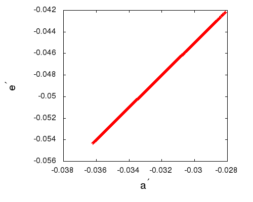
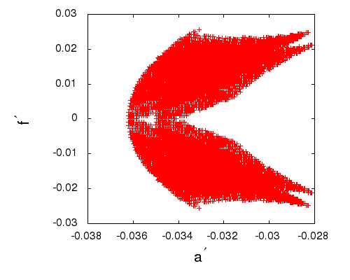
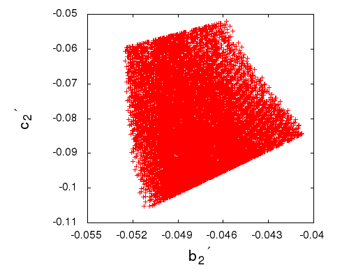
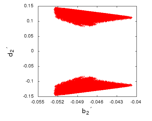
Figure 1: Case-I: Plots of the primed parameters for a normal mass hierarchy.

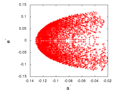
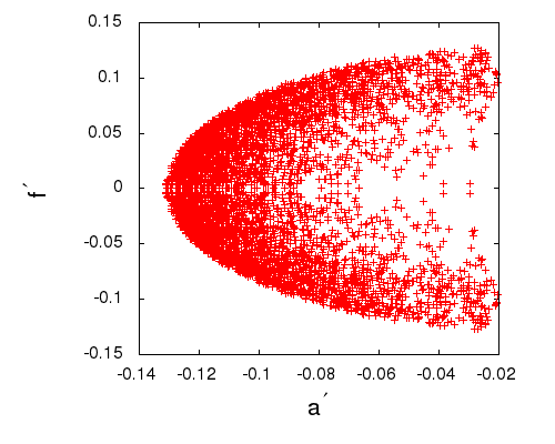
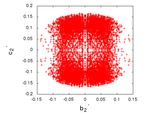
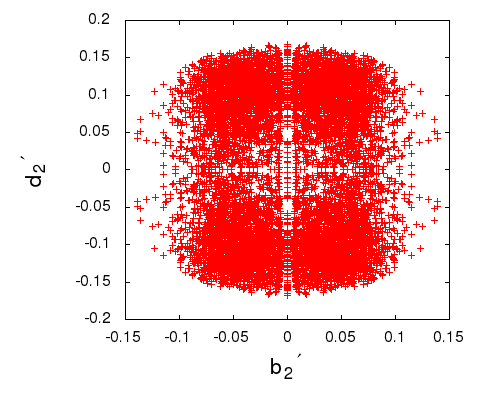
Figure 2: Case-I: Plots of the primed parameters for a inverted mass hierarchy.

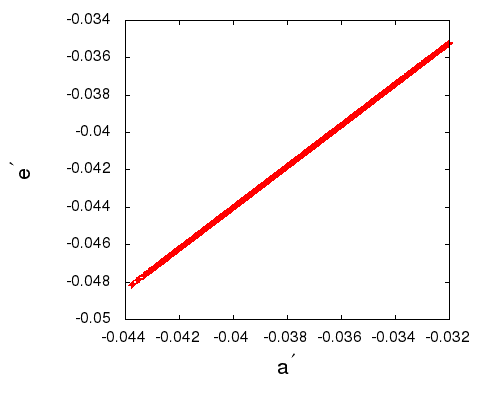
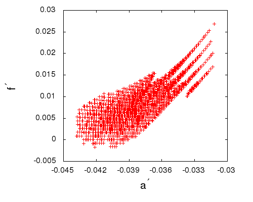
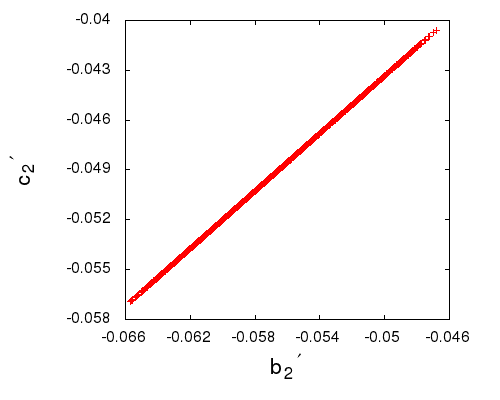
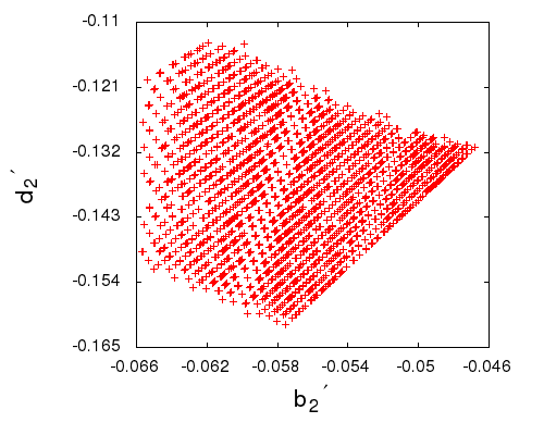
Figure 3: Case-II: Plots of the primed parameters for a normal mass hierarchy.

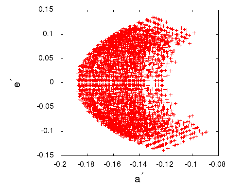
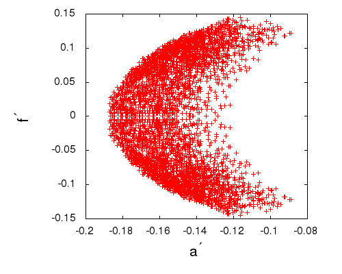
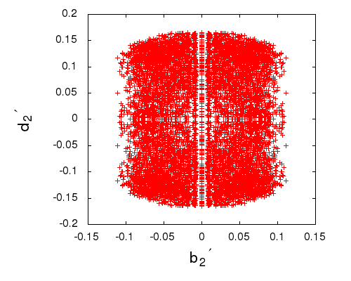
Figure 4: Case-II: Plots of the primed parameters for a normal mass hierarchy.

Table 3: Predictions on the light neutrino masses and $\sum_{i}m_{i}$.

Case-I
Normal Ordering			Inverted Ordering
$m_{1}/10^{-3}$	$m_{2}/10^{-3}$	$m_{3}/10^{-3}$	$m_{1}/10^{-3}$	$m_{2}/10^{-3}$	$m_{3}/10^{-3}$
$\rm(eV)$	$\rm(eV)$	$\rm(eV)$	$\rm(eV)$	$\rm(eV)$	$\rm(eV)$
$4.0-8.5$	$9.28-12.0$	$49-52$	$47-61$	$49-62$	$9-36$
$\sum_{i}m_{i}<0.08$ eV			$\sum_{i}m_{i}<0.16$ eV
Case-II
Normal Ordering			Inverted Ordering
$m_{1}/10^{-3}$	$m_{2}/10^{-3}$	$m_{3}/10^{-3}$	$m_{1}/10^{-3}$	$m_{2}/10^{-3}$	$m_{3}/10^{-3}$
$\rm(eV)$	$\rm(eV)$	$\rm(eV)$	$\rm(eV)$	$\rm(eV)$	$\rm(eV)$
$4.1-8.8$	$9.23-13.1$	$48-52$	$47-60$	$49-61$	$10-38$
$\sum_{i}m_{i}<0.08$ eV			$\sum_{i}m_{i}<0.16$ eV

Neutrinoless double beta decay ($\beta\beta_{0\nu}$)

This is a process arising from the decay of a nucleus as

$$(A,Z)\longrightarrow(A,Z+2)+2e^{-}$$ (5.2)

where the lepton number is violated by 2 units due to the absence of any final state neutrinos. Observation of such decay will lead to the confirmation of the Majorana nature of the neutrinos. The half-life[beta] corresponding to the above decay is given by

$$\frac{1}{T^{0\nu}_{1/2}}=G|\mathcal{M}|^{2}|M_{ee}|^{2}m_{e}^{-2},$$ (5.3)

where $G$ is the two-body phase space factor, $\mathcal{M}$ is the nuclear matrix element (NME), $m_{e}$ is the mass of the electron and $M_{ee}$ is the (1,1) element of the effective light neutrino mass matrix $M_{\nu}$. Using the PDG parametrization convention for $U_{PMNS}$[pdg], the $M_{ee}$ can be written as

$$M_{ee}=c_{12}^{2}c_{13}^{2}m_{1}+s_{12}^{2}c_{13}^{2}m_{2}e^{i\alpha}+s_{13}^{2}m_{3}e^{i(\beta-2\delta)}.$$ (5.4)

Significant upper limits on $|M_{ee}|$ are available from several ongoing experiments. Experiments such as KamLAND-Zen [kam] and EXO [exo] have constrained this value to be $<0.35$ eV. However, till date the most impressive upper bound of 0.22 eV on $|M_{ee}|$ is provided by GERDA phase-I data [gerda1] which is likely to be lowered even further by GERDA phase -II data[gerda2] to around 0.098 eV. As shown in Ref.[Rome], existence of $G_{3}^{(k)}$ in the neutrino mass matrix leads to four sets of values of the CP-violating Majorana phases $\alpha$ and $\beta$ for each neutrino mass ordering. Since $|M_{ee}|$ is sensitive to these phases, we get four different plots for each mass ordering. In Fig.5 we present the plots of $|M_{ee}|$ vs. the lightest neutrino mass ($m_{1,3}$) for both the mass orderings in Case-I only. Apart from slight changes in the upper and lower limits on $m_{1,3}$, Case-II also leads to similar plots since it also predicts same results on CP violating phases (i.e. $\cos\delta=0,\alpha,\beta=0~{}{\rm or}~{}\pi$).

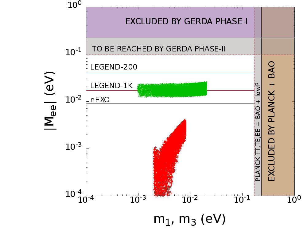
Figure 5: Plot of $|M_{ee}|$ vs. the lightest neutrino mass: the top two figures represent Case A: $\alpha=\pi$, $\beta=0$ (left) and Case B: $\alpha=\pi$, $\beta=\pi$ (right) while the figures in the lower panel represent Case C: $\alpha=0$, $\beta=0$ (left) and Case D: $\alpha=0$, $\beta=\pi$ (right).

This is evident from Fig.5 that $|M_{ee}|$ in each plot leads to an upper limit which is below the reach of the GERDA phase-II data. However, predictions of our model could be probed by GERDA + MAJORANA experiments [majo]. Sensitivity reach of other promising experiments such as LEGEND-200 (40 meV), LEGEND-1K (17 meV) and nEXO (9 meV)[Agostini:2017jim] are also shown in Fig.5. Note that for each case, the entire parameter space corresponding to the inverted mass ordering could be ruled out by the nEXO reach. One can also explain the nature of the plots analytically. Let us first consider the inverted mass ordering. In this case, with the approximations $m_{3}\simeq 0$ and $m_{1}\simeq m_{2}$, $|M_{ee}|$ simplifies to

$$|M_{ee}|=\sqrt{|\Delta m_{32}|^{2}}c_{13}^{2}[\{1-s_{12}^{2}(1-\cos\alpha)\}^{2}+s_{12}^{4}\sin^{2}\alpha]^{1/2}.$$ (5.5)

Clearly, $|M_{ee}|$ is not sensitive to the phases $\beta$ and $\delta$. On the other hand, for $\alpha=\pi$ and $0$ (5.5) further simplifies to

$$|M_{ee}|=\sqrt{|\Delta m_{32}|^{2}}c_{13}^{2}[\{1-2s_{12}^{2}\}^{2}]$$ (5.6)

and

$$|M_{ee}|=\sqrt{|\Delta m_{32}|^{2}}c_{13}^{2}$$ (5.7)

respectively. Therefore, for $\alpha=\pi$ (cases A, B), $|M_{ee}|$ is suppressed as compared to the case $\alpha=0$ (cases C, D). Now for a normal mass ordering, in addition to the $s_{13}$ suppression, there is a significant interference between the first two terms. If $\alpha=0$, the first two terms interfere constructively and we obtain a lower bound ($\sim 10^{-3}$ eV for Case C and $\sim 5\times 10^{-3}$ eV for Case D) despite it being a case of normal mass ordering of the light neutrinos. This is one of the crucial results of the present analysis. On the other hand, for $\alpha=\pi$, the first two terms interfere destructively and thus a sizable cancellation between them brings down the value of $|M_{ee}|$ and results in the kinks that is depicted in the lower curves in the top two figures.

Baryogenesis via flavored leptogenesis

As mentioned in the beginning of the numerical section, to get a positive $Y_{B}$, we were obliged to use those value of the primed parameters for which the low energy neutrino parameters predicted from our model lie close to their best fit values dictated by the oscillation experiment. To facilitate this purpose, we define a variable $\chi^{2}$ in Eq.(5.8) that measures the deviation of the parameters from their best fit values.

$$\chi^{2}=\sum\limits_{i=1}^{5}\Big{[}\frac{\mathcal{O}_{i}(th)-\mathcal{O}_{i}(bf)}{\Delta\mathcal{O}_{i}}\Big{]}^{2}.$$ (5.8)

In Eq.(5.8)) $\mathcal{O}_{i}$ denotes the $i^{th}$ neutrino oscillation observable among $\Delta m^{2}_{21},\Delta m^{2}_{32},\theta_{12},\theta_{23}$ and $\theta_{13}$ and the summation runs over all of them. The parenthetical $th$ stands for the numerical value of the observable given by our model, whereas $bf$ denotes the best fit value (cf. Table 2). $\Delta\mathcal{O}_{i}$ in the denominator stands for the measured $1\sigma$ range of $\mathcal{O}_{i}$. For numerical computation, we choose $M_{i+1}/M_{i}=10^{3}\hskip 2.84526pt(i=1,2)$. First we calculate $\chi^{2}$ as a function of the primed parameters in their constrained range. For a fixed value of $M_{1}$, we then start with the minimum value of $\chi^{2}$ and we keep on increasing it until $Y_{B}$ attains a positive value. For that particular $\chi^{2}$ i.e., for a particular set of primed parameters, we are then able to generate a large set of unprimed parameters by varying $M_{1}$ over a wide range and can calculate $Y_{B}$ for each value of $M_{1}$. Let’s discuss our results case by case for each mass ordering.

Case-I: $Y_{B}$ for normal mass ordering of light neutrinos:

$\bf{M_{1}<{10}^{9}}$ GeV:

In this regime, all three lepton flavors $(e,\mu,\tau)$ are distinguishable. Since $\varepsilon_{1}^{e}=0$, we need to individually evaluate $\varepsilon_{1}^{\mu,\tau}$ only. Numerically, the maximum value of $|\varepsilon_{1}^{\mu,\tau}|$ is found to be $\sim 10^{-8}$. $Y_{B}$ in the observed range cannot be generated with such a small CP asymmetry parameter. Theoretically, this can be understood as an interplay between various quantities. A unique feature in the present model is that the nonzero value of $\theta_{13}$ and $\varepsilon_{i}$ originated from the imaginary part of the $m_{D}$ matrix.

$\bf{{10}^{9}\,\,{\rm{\bf{{\rm GeV}}}}<M_{1}<{10}^{12}}$ GeV:

Before calculating final $Y_{B}$, we have to look first at the wash-out parameters $K_{\alpha}=\tilde{m}_{\alpha}/10^{-3}$ relevant to this mass regime. Since in this regime only $\tau$ flavor is distinguishable, there are two wash-out parameters, $K_{\tau}$ and $K_{2}=K_{e}+K_{\mu}$. As shown in the first plot of Fig.6, the entire range of these parameters is not much greater than 1 for the observed range of $Y_{B}$. Thus the efficiency factor in Eq.(4.16) can be written for this mild wash-out scenario[abada] as

$$\eta(\tilde{m}_{\alpha})=\Big{[}\Big{(}\frac{\tilde{m}_{\alpha}}{8.25\times 10^{-3}}\Big{)}^{-1}+\Big{(}\frac{0.2\times 10^{-3}}{\tilde{m}_{\alpha}}\Big{)}^{-1.16}\Big{]}^{-1}.$$ (5.9)

We then perform a $\chi^{2}$ scanning of the primed parameters. It has been found that for $\chi^{2}_{min}=0.083$ one can have $Y_{B}$ positive. Basically, In our scheme, Eq.(4.16) of the present manuscript can be written as

$$Y_{B}\simeq\frac{12}{37g^{*}}\varepsilon_{1}^{\mu}\Big{[}\eta\Big{(}\frac{390}{589}\tilde{m}_{\tau}\Big{)}-\eta\Big{(}\frac{417}{589}\tilde{m}_{2}\Big{)}\Big{]}.$$ (5.10)

Thus the sign of $Y_{B}$ depends upon the sign of $\varepsilon_{1}^{\mu}$ and the sign of the bracketed quantity. Now from the primed parameter space we take a particular set, calculate the corresponding $\chi^{2}$ and then compute $Y_{B}$. This has been seen that data sets corresponding to $\chi^{2}<0.083$ cannot produce positive $Y_{B}$, since for those data sets, we get positive values of $\varepsilon_{1}^{\mu}$ but negative values for the bracketed quantity. A complete data set of the primed parameters and corresponding values of the observables are tabulated in Table 4 for $\chi^{2}_{min}=0.083$. The other parameters i.e., $b_{1},c_{1},d_{1}$ can be calculated using Eq.(3.9)-(3.11).

Table 4: Parameters and observables corresponding $\chi^{2}=0.083$ for normal mass ordering.

$a^{\prime}$	$e^{\prime}$	$f^{\prime}$	$b_{2}^{\prime}$	$c_{2}^{\prime}$	$d_{2}^{\prime}$	$\chi^{2}$
$-0.036$	$-0.050$	$0.003$	$-0.052$	$-0.059$	$-0.122$	$0.083$
observables		$\theta_{13}$	$\theta_{12}$	$\theta_{23}$	$\Delta m_{21}^{2}\times 10^{5}$	$|\Delta m_{31}|^{2}\times 10^{3}$
$\chi^{2}=0.083$		$8.42^{0}$	$33.04^{0}$	$42.54^{0}$	$7.57~{}{\rm(eV)}^{2}$	$2.55~{}{\rm(eV)}^{2}$

Finally, given the primed data set for that $\chi^{2}_{min}$, $M_{1}$ is varied widely to have $Y_{B}$ in the observed range. For each value of $M_{1}$, a set of values of the unprimed parameters $\{a,e,f,b_{1},c_{1},d_{1},b_{2},c_{2},d_{2}\}$ is generated. Final $Y_{B}$ is then calculated for each values of $M_{1}$ and the corresponding unprimed set. A careful surveillance of the plot in Fig.7 leads to the conclusion that we can obtain an upper and a lower bound on $M_{1}$ due to the observed constraint on $Y_{B}$. In order to appreciate this fact more clearly, two straight lines have been drawn parallel to the abscissa in the mentioned plot: one at $Y_{B}=8.55\times 10^{-11}$ and the other at $Y_{B}=8.77\times 10^{-11}$. The values of $M_{1}$, where the straight lines meet the $Y_{B}$ vs $M_{1}$ curve, yield the allowed lower and upper bounds on $M_{1}$, namely $(M_{1})_{lower}=2.17\times 10^{11}$ GeV and $(M_{1})_{upper}=2.23\times 10^{11}$ GeV. To explain this linear correlation between $M_{1}$ and $Y_{B}$ one could see the expression for $\varepsilon_{1}^{\mu}$ in Eq.(LABEL:epsim). As we see from Eq.(LABEL:epsim), $\varepsilon_{1}^{\alpha}$ is composed of two terms. The first term is proportional to $M_{1}/M_{j}$ while the second term is proportional $(M_{1}/M_{j})^{2}$. Now for the assumed hierarchical scenario ($M_{3}\gg M_{2}\gg M_{1}$), the first term dominates (cf. Eq.LABEL:epssimp) and effectively $\varepsilon_{1}^{\alpha}$ becomes proportional to $M_{1}$ (theoretically which is not the case due to the presence of the second term). Now in Eq.(4.16), in the expression of $Y_{B}$, the wash-out parameters only depend upon the primed parameters. Thus effectively the final baryon asymmetry $Y_{B}$ is also proportional to $M_{1}$. One might also ask about the narrow range for $M_{1}$ as we see in the Fig.7. Basically we have presented our result for a particular set of primed parameters (for $\chi^{2}_{min}=0.083$). In principle one can take the entire primed parameter space of our model and compute the corresponding results on $Y_{B}$ and $M_{1}$ for each set of primed parameters. In that case (for the entire parameter space) the range of $M_{1}$ should not be as narrow as we see in this case.

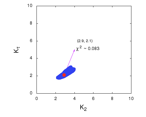
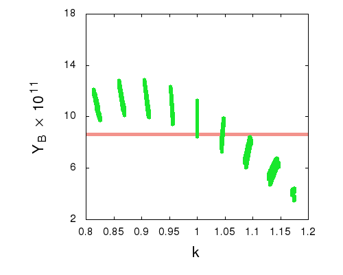
Figure 6: The plot on the left hand side shows the range of the wash-out parameters. The red dot corresponds to the minimum value of $\chi^{2}$ for which a set of primed parameters has been taken to compute $Y_{B}$. The plot on the right hand side shows a variation of $Y_{B}$ vs $k$. The red band in the same plot indicates the observed range of $Y_{B}$.

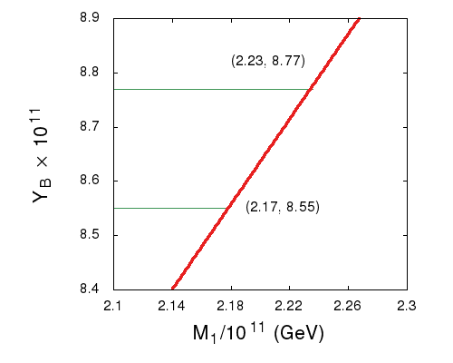
Figure 7: A plot of the final $Y_{B}$ for different values of $M_{1}$ for a normal light neutrino mass ordering.

From Table 4, we infer that $\theta_{23}=42.54^{0}$ corresponding to $\chi^{2}_{min}=0.083$. Since theoretically $\theta_{23}$ is related only with a single model parameter $k$ (cf. Eq.(2.20)) and unlike the other parameters of $m_{D}$ (discussed earlier in this section) value of $k$ does not depend upon the variation of $M_{1}$, $\theta_{23}$ remain fixed for the entire range of $M_{1}$ that corresponds to the observed range of $Y_{B}$. Thus an experimentally appealing conclusion of this scheme is that, given the observed range of $Y_{B}$, the octant of $\theta_{23}$ is determined ($<45^{0}$). One can also check the sensitivity of the produced $Y_{B}$ to the entire range of $\theta_{23}$ in a slightly different way. It is trivial to find out the analytic form of $Y_{B}$ that explicitly depend upon $\theta_{23}$, by replacing $k=(\tan\theta_{23})^{-1}$ in the expression of $\varepsilon_{1}^{\mu}$ and $m_{\alpha}$ in Eq.(5.10). Thus for a fixed value of $M_{1}$ one can use the entire parameter space of the primed parameters and $k$ to compute the final $Y_{B}$. From the plot on the right panel of Fig.6, we see that the value of $k$ is always greater that 1 for $Y_{B}$ to be in the observed range (represented by the red narrow strip in Fig.6). This is certainly for a particular value of $M_{1}(6.79\times 10^{11}{\rm GeV})$. As previously mentioned, $Y_{B}$ is almost proportional to $M_{1}$, thus lowering the value of the latter below $6.79\times 10^{11}{\rm GeV}$ would cause a downward movement of the overall pattern of the $Y_{B}$ vs. $k$ plot in Fig.6. Thus for the observed range of $Y_{B}$, along with the values $k>1$, there would be other values of $k$ which are less than one. It is seen that for the normal mass ordering in Case-II a similar lower limit on $M_{1}$ exist that dictates the octant of $\theta_{23}$ for the the observed range of $Y_{B}$.

We would like to stress that the lower bound obtained in the second approach is different from that is obtained in the first one. This is simply because the ways to obtain these bounds are different. In the first approach we take the best fit values of the primed parameters and $k$ and then vary $M_{1}$ to obtain the observed range of $Y_{B}$ which in turn leads to an upper and a lower bound on $M_{1}$. However, in the second approach, we take the entire primed parameter space along with the allowed range for $k$ and then compute $Y_{B}$ for a fixed value of $M_{1}$. The $Y_{B}$ vs. $k$ plot in Fig.6 is for $M_{1}=6.79\times 10^{11}{\rm GeV}$ which represents the lower bound on $M_{1}$ above which we always get $k>1$ for the observed range of $Y_{B}$. Now what happens if we further lower the value of $M_{1}$ from $6.79\times 10^{11}{\rm GeV}$ in the second approach? As discussed previously, this would imply a downward movement of $Y_{B}$ vs $k$ curve in Fig.6 or in Fig.9. In that case both $k>1$ and $k<1$ values are possible for the observed range of $Y_{B}$. Obviously this has an impact on the results obtained in the first method. We know from the first method that if we choose the best fit value of $k$, the allowed range of $M_{1}$ should be read from Fig.7. This does not necessarily mean that for this range of $M_{1}$, other values of $k$ are not possible (obviously those values of $k$ should not be the best fit values then) since the range shown in Fig.7 is below $M_{1}=6.79\times 10^{11}$ GeV.

$\bf{M_{1}>{10}^{12}}$ GeV:

It has been shown that $Y_{B}=0$ here for our model.

Case-I: $Y_{B}$ for inverted mass ordering of light neutrinos:

Following the same procedure as for the normal mass ordering, a final discussion for each regime is summarized as follows.

${\bf{M_{1}<{10}^{9}}}$ GeV:

Similar to the normal ordering, the $|\varepsilon_{1}^{\mu,\tau}|$ can have values at most the order of $10^{-8}$ which is not sufficient to let $Y_{B}$ come within its observed range.

$\bf{{10}^{9}\,\,{\rm{\bf{{\rm GeV}}}}<M_{1}<{10}^{12}}$ GeV:

Unlike the previous case the ranges of the the wash-out parameters (cf. Fig.8) favors a strong wash-out scenario.

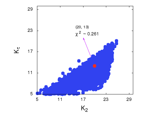
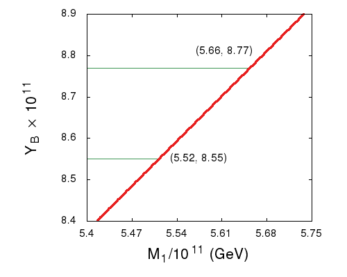
Figure 8: The plot on the left hand side shows the range of the wash-out parameters. The red dot corresponds to the minimum value of $\chi^{2}$ for which a set of primed parameter has been taken to compute $Y_{B}$. The plot on the right hand side shows final $Y_{B}$ for different values of $M_{1}$ for the inverted light neutrino mass ordering.

Thus the efficiency factor in Eq.(4.16) can be written for this strong wash-out scenario[abada]as

$$\eta(\tilde{m}_{\alpha})=\Big{[}\Big{(}\frac{0.55\times 10^{-3}}{\tilde{m}_{\alpha}}\Big{)}^{1.16}\Big{]}.$$ (5.11)

For $\chi^{2}_{min}=0.261$, a set of primed parameters is obtained (cf. Table 5). Then similar to the previous case, varying $M_{1}$ in a wide range, a lower and upper bound on $M_{1}$, namely $(M_{1})_{lower}=5.52\times 10^{11}$ GeV and $(M_{1})_{upper}=5.66\times 10^{11}$ GeV is obtained for the observed range of $Y_{B}$. A plot of $Y_{B}$ vs $M_{1}$ is shown in the right panel of Fig.8.

Table 5: Parameters and observables corresponding $\chi^{2}=0.261$ for inverted hierarchy.

$a^{\prime}$	$e^{\prime}$	$f^{\prime}$	$b_{2}^{\prime}$	$c_{2}^{\prime}$	$d_{2}^{\prime}$	$\chi^{2}$
$-0.043$	$-0.065$	$0.116$	$0.130$	$-0.019$	$0.039$	$0.261$
observables		$\theta_{13}$	$\theta_{12}$	$\theta_{23}$	$\Delta m_{21}^{2}\times 10^{5}$	$|\Delta m_{31}|^{2}\times 10^{3}$
$\chi^{2}=0.261$		$8.54^{0}$	$34.07^{0}$	$49.37^{0}$	$7.53~{}{\rm(eV)}^{2}$	$2.40~{}{\rm(eV)}^{2}$

$\bf{M_{1}>{10}^{12}}$ GeV:

Once again, $Y_{B}=0$ in this regime, for the present model.

Case-II: $Y_{B}$ for normal mass ordering of light neutrinos:

The analysis has been done exactly in the same way as was in the previous case. A systematic presentation of the obtained results is the following.

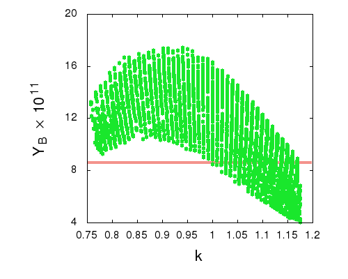
Figure 9: The plot on the left hand side shows the range of the wash-out parameters. The red dot corresponds to the minimum value of $\chi^{2}$ for which a set of primed parameter has been taken to compute $Y_{B}$. The plot on the right hand side shows a variation of $Y_{B}$ vs $k$. The red band in the same plot indicates the observed range of $Y_{B}$.

$\bf{M_{1}<{10}^{9}}$ GeV:

Again, $Y_{B}$ in the observed range cannot be generated due to the small value of $|\varepsilon_{1}^{\mu,\tau}|$.

$\bf{{10}^{9}\,\,{\rm{\bf{{\rm GeV}}}}<M_{1}<{10}^{12}}$ GeV:

Similar to the previous normal hierarchical case, the wash-out parameters here also suggest a mild wash-out scenario (cf. Fig.9).

For $\chi^{2}_{min}=0.256$, a set of rescale parameter has been found and then varying $M_{1}$ in a wide range, a lower and a upper bound on $M_{1}$ are obtained as shown in the Fig.10. Note that in this case also $\theta_{23}<45^{0}$ (Table 6) for the minimum $\chi^{2}$ that produce $Y_{B}$ positive and in the observed range. Similar to the case of normal mass ordering in Case-I, here we also show a $Y_{B}$ vs $k$ plot (cf. Fig.9) and infer that there exists a lower limit $8.2\times 10^{11}{\rm GeV}$ on $M_{1}$ for which $k>1$, i.e., $\theta_{23}<45^{0}$ for $Y_{B}$ to be in the observed range.

Table 6: Parameters and observables corresponding $\chi^{2}=0.256$ for normal mass ordering.

$a^{\prime}$	$e^{\prime}$	$f^{\prime}$	$b_{2}^{\prime}$	$c_{2}^{\prime}$	$d_{2}^{\prime}$	$\chi^{2}$
$-0.042$	$-0.046$	$-0.005$	$-0.065$	$-0.056$	$-0.128$	$0.256$
observables		$\theta_{13}$	$\theta_{12}$	$\theta_{23}$	$\Delta m_{21}^{2}\times 10^{5}$	$|\Delta m_{31}|^{2}\times 10^{3}$
$\chi^{2}=0.256$		$8.37^{0}$	$33.08^{0}$	$43.49^{0}$	$7.55~{}{\rm(eV)}^{2}$	$2.55~{}{\rm(eV)}^{2}$

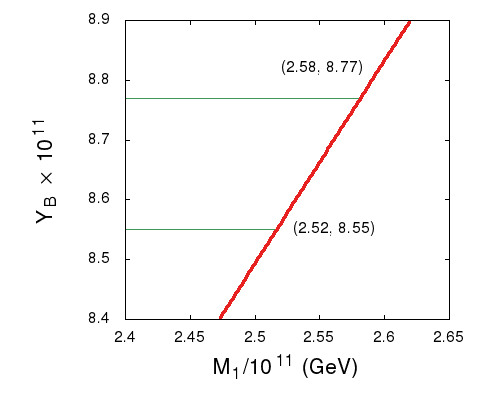
Figure 10: A plot of the final $Y_{B}$ for different values of $M_{1}$ for the normal light neutrino mass ordering.

$\bf{M_{1}>{10}^{12}}$ GeV:

It has been shown that $Y_{B}=0$ here for our model.

Case-II: $Y_{B}$ for inverted mass ordering of light neutrinos:

Proceeding exactly in the same manner as for the normal mass ordering, a brief discussion for each regime goes as follows.

${\bf{M_{1}<{10}^{9}}}$ GeV:

Similar to the normal ordering, the $|\varepsilon_{1}^{\mu,\tau}|$ can have values at most the order of $10^{-8}$ which is not sufficient to let $Y_{B}$ come within its observed range.

$\bf{{10}^{9}\,\,{\rm{\bf{{\rm GeV}}}}<M_{1}<{10}^{12}}$ GeV:

Unlike the previous case the ranges of the wash-out parameters (cf. Fig.11) favors a strong wash-out scenario. For $\chi^{2}_{min}=0.041$ a set of primed parameters is obtained (cf Table 7). Then similar to the previous case varying $M_{1}$ in a wide range a lower and upper bound on $M_{1}$, namely $(M_{1})_{lower}=5.27\times 10^{11}$ GeV and $(M_{1})_{upper}=5.40\times 10^{11}$ GeV is obtained for the observed range of $Y_{B}$. A plot of $Y_{B}$ vs $M_{1}$ is shown in the right panel of Fig.11.

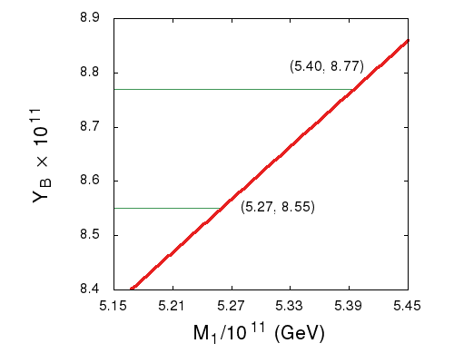
Figure 11: The plot on the left hand side shows the range of the wash-out parameters. The red dot corresponds to the minimum value of $\chi^{2}$ for which a set of primed parameter has been taken to compute $Y_{B}$. The plot on the right hand side shows final $Y_{B}$ for different values of $M_{1}$ for the inverted light neutrino mass ordering.

Table 7: Parameters and observables corresponding $\chi^{2}=0.041$ for inverted hierarchy.

$a^{\prime}$	$e^{\prime}$	$f^{\prime}$	$b_{2}^{\prime}$	$c_{2}^{\prime}$	$d_{2}^{\prime}$	$\chi^{2}$
$-0.123$	$-0.084$	$0.123$	$0.104$	$-0.052$	$-0.096$	$0.041$
observables		$\theta_{13}$	$\theta_{12}$	$\theta_{23}$	$\Delta m_{21}^{2}\times 10^{5}$	$|\Delta m_{31}|^{2}\times 10^{3}$
$\chi^{2}=0.041$		$8.71^{0}$	$33.43^{0}$	$49.23^{0}$	$7.58~{}{\rm(eV)}^{2}$	$2.44~{}{\rm(eV)}^{2}$

$\bf{M_{1}>{10}^{12}}$ GeV:

Once again, $Y_{B}=0$ here for the present model.

A compact presentation of the final conclusions regarding $Y_{B}$ from the numerical analysis is given in Table 5.

Table 8: Final statements on $Y_{B}$ for different mass regimes.

Case-I
${\rm Type}$	${M_{1}<10^{9}\hskip 2.84526pt{\rm GeV}}$	$10^{9}\hskip 2.84526pt{\rm GeV}<M_{1}<10^{12}\hskip 2.84526pt{\rm GeV}$	${M_{1}>10^{12}\hskip 2.84526pt{\rm GeV}}$
$\pbox{20cm}$
Ordering	$\pbox{20cm}$
is below the observed range
for any $\chi^{2}$.$&$20cm$Y_{B}$ within  the  observed   range
for $\chi^{2}_{min}=0.083$.$&$20cmRuled out
since $Y_{B}=0.$${\\ }{\cline{1-4}}\vrule\lx@intercol\hfil$\pbox{20cm}$
Ordering	20cmRuledoutsinceYB
isbelowtheobserv