Higher-order meshing of implicit geometries—part III:
Conformal Decomposition FEM (CDFEM)

T.P. Fries

Abstract

A higher-order accurate finite element method is proposed which uses automatically generated meshes based on implicit level-set data for the description of boundaries and interfaces in two and three dimensions. The method is an alternative for fictitious domain and extended finite element methods. The domain of interest is immersed in a background mesh composed by higher-order elements. The zero-level sets are identified and meshed followed by a decomposition of the cut background elements into conforming sub-elements. Adaptivity is a crucial ingredient of the method to guarantee the success of the mesh generation. It ensures the successful decomposition of cut elements and enables improved geometry descriptions and approximations. It is confirmed that higher-order accurate results with optimal convergence rates are achieved with the proposed conformal decomposition finite element method (CDFEM).

Keywords: higher-order FEM, level-set method, fictitious domain method, embedded domain method, immersed boundary method, XFEM, GFEM, interface capturing

Institute of Structural Analysis

Graz University of Technology

Lessingstr. 25/II, 8010 Graz, Austria

www.ifb.tugraz.at
fries@tugraz.at

1 Introduction

The $p$ -version of the finite element method ( $p$ -FEM) enables a higher-order accurate and efficient approximation of boundary value problems (BVPs) in engineering, natural sciences, and related fields [50, 6, 8, 58, 55]. Two crucial requirements are needed for the successful application of the $p$ -FEM: (i) The geometry must be accurately represented by a mesh composed of higher-order elements and (ii) the solution of the BVP should be sufficiently smooth. Both requirements are not easily met. For (i), curved boundaries and interfaces in the domain of interest may render the mesh generation difficult, in particular in three dimensions and with elements of higher orders. Even more so when frequent mesh manipulations are desired, for instance, in the context of moving interfaces (interface tracking) or mesh refinements in adaptivity and convergence studies. The original geometry is often generated based on Computer Aided Geometric Design (CAGD or CAD) and the interplay with the analysis tool, i.e., the $p$ -FEM, is not easily established and hardly automated. Concerning (ii), the smoothness of the involved fields in the BVP, it is noted that discontinuities (e.g., in the material parameters) and singularities (e.g., in the stress field of a structure) are frequently present. For the successful application of the $p$ -FEM in these cases, it is again crucial to provide suitable meshes, i.e., those which conform to the discontinuities and are refined at the singularities. It is thus seen that a lot of effort is associated to generating higher-order accurate meshes as properties of the geometry and the approximated solutions must both be considered.

Herein, the focus is on the automatic, higher-order accurate generation of conforming meshes based on implicitly defined geometries. The domain of interest is completely immersed in a background mesh. The boundary of the domain and interfaces therein, for example, between different materials, are defined by (several) level-set functions [42, 41, 48]. For each level-set function, the elements cut by the zero-level set are decomposed into conforming, higher-order sub-elements. Therefore, the zero-level set is first identified and meshed by interface elements (reconstruction) and then customized mappings generate the sub-elements (decomposition). This follows previous works of the author in [21, 18, 22] where the resulting meshes are used in the context of integration and interpolation in implicitly defined domains. However, in elements where the decomposition fails, e.g., due to very complex level-set data, (isolated) recursive refinements were suggested and hanging nodes are a natural consequence. Herein, we wish to use the generated meshes in the context of approximating BVPs and hanging nodes shall be avoided. The quality of the generated sub-elements becomes an important issue in this context. Following [31, 27], node manipulations in the background mesh are suggested to ensure suitable, shape-regular elements. One may also possibly use stabilizations similar to those suggested in [10, 11, 9, 25].

Adaptive refinements of the background mesh are suggested in order to (i) refine elements where the decomposition failed, (ii) improve the geometry description driven by the curvature of the involved level-set functions near the zero-level sets, (iii) improve the approximation of the BVP, for example, based on error indicators. Because “good” meshes must consider both, the geometry and the involved (sought) fields of the BVP, adaptivity is a natural ingredient for automatic mesh generation without any user intervention. Hence, the suggested procedure follows the isogeometric paradigm [26, 33] to fully integrate design and analysis, however, for implicit geometries rather than based on NURBS as in CAGD.

The fully automatic generation of meshes based on implicit level-set data is gaining increasing attention. We emphasize the work of [39] in a low-order context for moving interfaces which coined the name CDFEM. A higher-order extension of this work in two dimensions is found in [40] without adaptive refinements and measures to avoid ill-shaped elements. This is the first work where the CDFEM is extended to higher-order consistently in two and three dimensions, including adaptivity and node manipulations to ensure the regularity of the resulting elements. The resulting method is stable and efficient.

The decomposition of elements is frequently employed in the context of “fictitious domain methods” (FDMs) such as the unfitted or cut finite element method [10, 11, 9, 25], finite cell method [2, 16, 43, 46, 47], Cartesian grid method [56, 57], immersed interface method [29], virtual boundary method [45], embedded domain method [32, 38] etc. The important difference between the CDFEM and FDMs is that the first uses the shape functions of the decomposed elements in the conforming mesh as the approximation basis whereas the second employs the shape functions of the original background mesh and uses the sub-elements for integration purposes only. Integration in cut elements using element decompositions is suggested in [1, 37, 15] using polygonal sub-cells together with recursive refinements. Curved sub-cells based on higher-order elements are, e.g., used in [28, 12, 21, 22] and typically lead to much less integration points. The integration schemes based on element decompositions are also frequently employed in the context of the extended or generalized finite element methods (XFEM/GFEM), see e.g., [7, 35, 20] for the XFEM and [51, 52] for the GFEM. They consider for inner-element jumps and kinks by adding enrichment functions based on the partition of unity concept [4, 5, 34]. Again, in these methods the decomposed sub-elements are only used as integration cells without using the implied shape functions for the approximation of the BVP.

It is emphasized that the proposed higher-order accurate CDFEM may be seen as an alternative for FDMs where boundaries are defined implicitly and the XFEM where interfaces are defined implicitly. The numerical results show typical applications of FDMs and the XFEM in two and three dimensions and higher-order convergence rates are achieved.

The paper is organized as follows: In Section 2, the concept of background meshes and their interaction with the implicitly defined boundaries and interfaces based on level-set functions is introduced and the procedure to decompose cut elements into conforming sub-elements based on [21, 22] is summarized. Section 3 details the adaptive refinement strategy in elements where the decomposition fails and, in addition, to improve the geometry representation and approximation properties. From the resulting set of elements, the generation of a finite element mesh including the connectivity information is outlined in Section 4. A node manipulation scheme to ensure the shape-regularity of the generated elements is described there as well. The proposed higher-order CDFEM is very general, however, herein it is applied in the context of solid mechanics with the governing equations as given in Section 5. Numerical results in two and three dimensions are presented in Section 6 where typical applications of FDMs and XFEM are considered with the proposed higher-order CDFEM. Finally, the paper ends with a summary and conclusion in Section 7.

2 Preliminaries

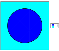
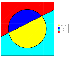
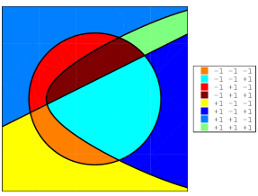
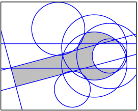
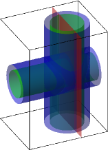
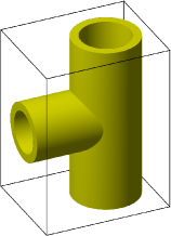
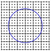
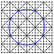
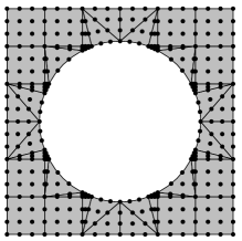
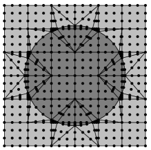
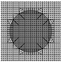
Starting point is a domain of interest $\Omega$ in two or three dimensions which is fully immersed in a background mesh composed by (possibly unstructured) higher-order Lagrange elements. The boundary of the domain and/or interfaces therein, for example between different materials, are defined by the zero-contours of the level-set functions $\phi_{i}\left(\mathchoice{\displaystyle\boldsymbol{x}}{\textstyle\boldsymbol{x}}{\scriptstyle\boldsymbol{x}}{\scriptscriptstyle\boldsymbol{x}}\right)$ . The level-set functions are evaluated at the nodes of the background mesh and, inbetween, interpolated by $\phi_{i}^{h}\left(\mathchoice{\displaystyle\boldsymbol{x}}{\textstyle\boldsymbol{x}}{\scriptstyle\boldsymbol{x}}{\scriptscriptstyle\boldsymbol{x}}\right)$ based on classical finite element shape functions. The signs of the level-set functions define sub-regions in the background mesh and it is easily verified that $k$ level-set functions may identify a maximum of $2^{k}$ subregions, see Fig. 1(a) to (c). It is important to note that several level-set functions naturally imply corners and edges of the domain of interest which has already been discussed in [22]. Consequently, a purely implicit description of complex geometries of practical interest is possible using multiple level-set functions. See Fig. 2 for some examples where several zero-level sets in two and three dimensions are shown and the implied geometries are highlighted.

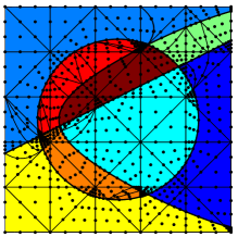
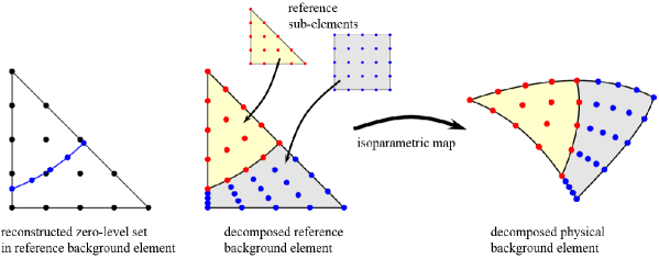
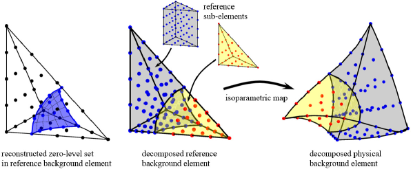
The task is to automatically generate higher-order meshes which conform to the boundaries and interfaces defined by the zero-level sets, see e.g., Fig. 1(d). Based on the sign-combinations of the involved level-set functions, void regions are easily identified and/or material properties assigned. The mesh generation with respect to all level-set functions is realized one after the other. For each level-set function, the following steps are performed for every elements, see Fig. 3 and references [21, 22] for further details:

1.

Detection whether the element is cut by the current level-set function or not. This is based on a sample grid because nodal values are not sufficient for this decision. For cut elements proceed with step 2, otherwise with the next element.
2.

Determine how the zero-level set cuts the element and classify the topological cut situation provided that the level-set data is not too complex, see below.
3.

Reconstruction: In the reference element, identify the zero-level set and define interface elements. Therefore, element nodes are identified on the zero-level set along specified search paths for which a tailored Newton-Raphson scheme is employed. The definition of such search paths and the corresponding start values for the iteration are crucial for the success.
4.

Decomposition: Decompose the reference element based on the reconstructed interface element wherefore customized mappings of sub-elements are employed depending on the topological cut situation.
5.

Map the decomposed sub-elements from the reference to the physical background element.

Note that these steps do not necessarily lead to a successul decomposition of an element. For example, (a) the zero-level set may be too complex and cuts the element several times so that no standard topological cut situation is present, (b) the identified nodes on the zero-level set are outside the element, or (c) the Jacobian of a decomposed sub-element may be negative, hence, invalid. Therefore, it was suggested in [21, 22] to use recursive refinements of the element until the reconstruction and decomposition are successful. As a consequence, some of the resulting sub-elements feature hanging nodes so that such meshes are “irregular”. This is not a problem in an integration and interpolation context as in [21, 22], however, in the context of approximating BVPs, it is highly benefitial to have regular meshes without hanging nodes. Hence, herein we wish to avoid recursive refinements in the sense of [21, 22] and suggest to use adaptive mesh refinements instead, which enables the generation of regular, conforming meshes.

3 Adaptive mesh refinements

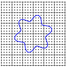
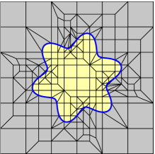
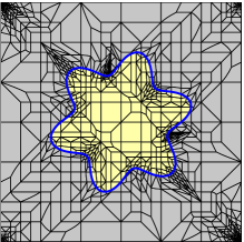
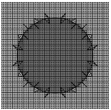
The decomposition of all cut elements of a background mesh yields a regular mesh without hanging nodes provided that (i) the background mesh itself is regular and (ii) the decompositions may be successfully realized in all cut elements. However, the second criterion cannot, in general, be guaranteed and there is typically a small number of background elements where the decomposition fails even for smooth level-set data. Those elements have to be refined and, in order to still meet criterion (i), also some neighboring elements of the background mesh are affected. This is shown in Fig. 4 for an extreme case where a very coarse background mesh is used for a rather complex zero-level set. An (unusual) large number of elements has to be refined because the decomposition fails for reasons mentioned above, see Fig. 4(b). Sometimes, even further refinement steps are required for an original background element until, finally, the decomposition of all refined sub-elements is valid. It is also clearly seen, that the refined background mesh is regular, for which neighboring elements may have to be refined as well (although they are not even cut by the zero-level set).

We find that at least for two further reasons, adaptive refinements of the background mesh may be useful: to better capture the geometry of the boundaries and interfaces and, in the context of approximating BVPs, to improve the approximation. To improve the geometry description it is useful to employ a curvature criterion in cut elements: The curvature $\varkappa$ of the level-set function is evaluated in the element and compared to the “element length” $h$ . We use the mean curvature, defined in two and three dimensions as

	$\displaystyle\varkappa_{\mathrm{2D}}$	$\displaystyle=$	$\displaystyle\dfrac{\phi_{,xx}\cdot\phi_{,y}^{2}-2\phi_{,x}\phi_{,y}\phi_{,xy}+\phi_{,yy}\cdot\phi_{,x}^{2}}{\left(\phi_{,x}^{2}+\phi_{,y}^{2}\right)^{\nicefrac{{3}}{{2}}}},$
	$\displaystyle\varkappa_{\mathrm{3D}}$	$\displaystyle=$	/12 $\cdot\dfrac{\begin{array}[]{c}\left(\phi_{,yy}+\phi_{,zz}\right)\cdot\phi_{,x}^{2}+\left(\phi_{,xx}+\phi_{,zz}\right)\cdot\phi_{,y}^{2}+\left(\phi_{,xx}+\phi_{,yy}\right)\cdot\phi_{,z}^{2}\\ -2\phi_{,x}\phi_{,y}\phi_{,xy}-2\phi_{,x}\phi_{,z}\phi_{,xz}-2\phi_{,y}\phi_{,z}\phi_{,yz}\end{array}}{\left(\phi_{,x}^{2}+\phi_{,y}^{2}+\phi_{,z}^{2}\right)^{\nicefrac{{3}}{{2}}}}.$

The element length may be the maximum Euclidean distance between every pair of corner nodes of a physical element. One may then use the criterion

\dfrac{1}{\varkappa}\leq q\cdot h\qquad\text{with}\qquad 0<q\in\mathbb{R}<2

(3.2)

to mark elements for refinement. The value $q$ tunes the criterion between $0$ for no curvature-driven refinement to $2$ (or larger) for typically very curvature-sensitive refinements in cut elements. An example for $q=0.6$ is shown in Fig. 4(c).

Finally, adaptivity may also be useful when the automatically generated, conforming meshes resulting from the previous steps are employed in the context of approximating BVPs. This is the classical application of adaptivity in the FEM, see e.g., [3, 13, 14, 50]. Although hanging nodes in the refined meshes are avoided herein, they do not, in general, pose insurmountable problems in classical $hp$ -FEM, see e.g., [49, 36]. The refinement criteria may be based on error indicators or heuristic criteria such as near reentrant corners where singularities are expected. Algorithmically, when adaptive refinements are already implemented for the reasons mentioned above, it is only little effort to also enable adaptivity to improve approximations. To continue the schematic example from above, see Fig. 4(d) where a refinement has been realized in the corners of the square domain, for example, because singularities are expected there for point supports in a solid mechanics context.

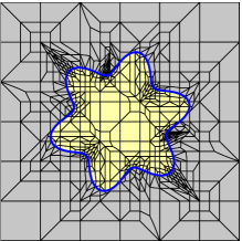
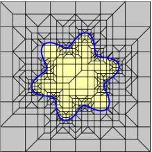
It is noted that adaptivity with respect to elements where the decomposition fails and those where the curvature criterion from Eq. (3.2) fails, may easily be combined in one element loop. It is recommended to first check the curvature criterion and only try the decomposition when the curvature of the level-set function is sufficiently small with respect to the element size. It is then typical that the decomposition fails in less than $1\%$ of the elements. Note that the order of the adaptive refinements is not commutative. Fig. 4(e) shows the resulting mesh when the curvature criterion is enforced first followed by the decomposition; only very few elements have to be further refined then. It is obvious that this leads to a superior mesh than in Fig. 4(c) where refinements have first been made to enable the decomposition and, thereafter, to enforce the curvature criterion.

4 Mesh generation

The procedure from above yields a set of higher-order elements conforming to the inner-element boundaries and/or interfaces, yet without information on the inter-element connectivity. It is important to ensure that across element boundaries, the generated element nodes are exactly at the same positions. For example, in three dimensions it may be useful to first generate element nodes on the element faces (achieved in 2D reference elements and mapped to the physical face element), generating a wireframe model of the zero-level sets. Next, the inner element nodes are generated based on 3D reference elements mapped to the physical background elements. It is then simple to generate the connectivity of the nodes needed for the complete definition of a finite element mesh. It is noted that the resulting meshes are mixed, e.g., in two dimensions, they are composed by triangular and quadrilateral Lagrange elements. Of course this could be avoided by converting elements to one type only.

With each element, we store the information of the signs of all level-set functions needed for the definition of boundaries and interfaces. Based on this information, one may easily identify elements that are outside the domain of interest or associate material properties in individual sub-regions of the domain.

Valid meshes for the approximation of BVPs must feature shape regular elements. However, this cannot generally be guaranteed for arbitary level-set data on a given background mesh. Therefore, we suggest to move nodes of the background mesh to ensure the shape regularity. The aim is to bound the areas/volumes of the elements from below. This is ensured by moving corners nodes of the elements away from the zero-level sets. Only the nodes in a close band around the zero isosurface are moved. The procedure was described by the author in detail in [23] and is only outlined here. It is applied before the decomposition is started (however, after a potential adaptive refinement of the background mesh due to the curvature criterion from above). It is also noted that [31, 27] suggest node manipulations in related contexts, however, the concrete algorithm from [23] and herein is quite different.

The procedure of the node manipulations is split into the following steps which are realized successively for all level-set functions involved: (i) The distance of the nodes to the zero-level set is approximated using a Newton-Raphson-type approach (this step is not needed when the level-set functions feature signed-distance property). (ii) The direction to the corresponding node on the zero-level set is measured. This is not necessarily the exact shortest distance, however, it will be a good approximation for nodes which are close to the zero-level set. (iii) If the distance is below a given threshold depending on the element length $h$ , the node is moved away from the zero-level set. The moving distance depends on the distance itself and is ramped linearly within the narrow band around the zero-level set. The procedure (i) to (iii) is repeated resulting in a fix-point iteration. For further details, see [23]. Examples of manipulated background meshes are seen in Fig. 5. We note that the node manipulations must be sufficiently small to maintain the validity of the background mesh which is not a problem in general. In particular the concept of “universal meshes” [44] allows for a large range of manipulations of individual nodes without leading to invalid elements (with negative Jacobians).

We summarize the differences between the proposed strategy to automatically generate valid finite element meshes for approximations compared to those decompositions needed only for integration purposes, e.g., in the context of the XFEM and FDMs as proposed in [21, 22]. Here, regular adaptive refinements are suggested in contrast to recursive refinements that generate hanging nodes. A node manipulation scheme is used to ensure the shape regularity which was not a concern in the integration context. The generated elements must be $C_{0}$ -continuous whereas they may be discontinuous for the numerical integration. It is noted that the related method suggested in [40] is (i) only two-dimensional, (ii) avoids refinements for the price of more topologically different decompositions of cut elements into sub-elements, and (iii) does not describe the issue of node manipulations. Core features of the proposed method herein are adaptivity, node manipulations, a simple decomposition into a minimal number of sub-elements, and a consistent, similar treatment in two and three dimensions.

5 Governing Equations of Linear Elasticity

The proposed higher-order CDFEM is applicable for the approximation of general BVPs when inner-element boundaries and interfaces are present and manufactured meshes are to be avoided. Herein, as a representative field of application, we focus on structural mechanics and linear elasticity. The corresponding governing equations are presented within this section.

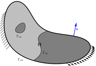
A domain of interest $\Omega$ in two or three dimensions is considered which is completely immersed in a background domain $\Omega_{\mathrm{BG}}$ . The boundary of $\Omega$ may be called external interface $\Gamma_{\mathrm{ext}}$ and interfaces within $\Omega$ , e.g., between different materials, are called internal, $\Gamma_{\mathrm{int}}$ . Displacements are continuous accross $\Gamma_{\mathrm{int}}$ , however, stresses and strains are discontinuous there. External and internal interfaces are implied by zero-level sets as described above. See Fig. 6 for a sketch of the situation in two dimensions.

The boundary $\Gamma_{\mathrm{ext}}$ is decomposed into the complementary sets $\Gamma_{\mathchoice{\displaystyle\boldsymbol{u}}{\textstyle\boldsymbol{u}}{\scriptstyle\boldsymbol{u}}{\scriptscriptstyle\boldsymbol{u}}}$ and $\Gamma_{\mathchoice{\displaystyle\boldsymbol{t}}{\textstyle\boldsymbol{t}}{\scriptstyle\boldsymbol{t}}{\scriptscriptstyle\boldsymbol{t}}}$ . Displacements $\hat{\mathchoice{\displaystyle\boldsymbol{u}}{\textstyle\boldsymbol{u}}{\scriptstyle\boldsymbol{u}}{\scriptscriptstyle\boldsymbol{u}}}$ are prescribed along the Dirichlet boundary $\Gamma_{\mathchoice{\displaystyle\boldsymbol{u}}{\textstyle\boldsymbol{u}}{\scriptstyle\boldsymbol{u}}{\scriptscriptstyle\boldsymbol{u}}}$ , and tractions $\hat{\mathchoice{\displaystyle\boldsymbol{t}}{\textstyle\boldsymbol{t}}{\scriptstyle\boldsymbol{t}}{\scriptscriptstyle\boldsymbol{t}}}$ along the Neumann boundary $\Gamma_{\mathchoice{\displaystyle\boldsymbol{t}}{\textstyle\boldsymbol{t}}{\scriptstyle\boldsymbol{t}}{\scriptscriptstyle\boldsymbol{t}}}$ . The strong form for an elastic solid undergoing small displacements and strains under static conditions, is [8, 58]

\nabla\cdot\boldsymbol{\sigma}=\mathchoice{\displaystyle\boldsymbol{f}}{\textstyle\boldsymbol{f}}{\scriptstyle\boldsymbol{f}}{\scriptscriptstyle\boldsymbol{f}},\quad\mathrm{on}\,\,\Omega\subseteq\mathbb{R}^{2},

(5.1)

where $\mathchoice{\displaystyle\boldsymbol{f}}{\textstyle\boldsymbol{f}}{\scriptstyle\boldsymbol{f}}{\scriptscriptstyle\boldsymbol{f}}$ describe volume forces, and $\boldsymbol{\sigma}$ is the following stress tensor

\boldsymbol{\sigma}=\mathchoice{\displaystyle\mathbf{C}}{\textstyle\mathbf{C}}{\scriptstyle\mathbf{C}}{\scriptscriptstyle\mathbf{C}}:\boldsymbol{\varepsilon}=\lambda\left(\textrm{tr}\,\boldsymbol{\varepsilon}\right)\mathchoice{\displaystyle\mathbf{I}}{\textstyle\mathbf{I}}{\scriptstyle\mathbf{I}}{\scriptscriptstyle\mathbf{I}}+2\mu\boldsymbol{\varepsilon},

(5.2)

with $\lambda$ and $\mu$ being the Lamé constants which are easily related to Young’s modulus $E$ and Poisson’s ratio $\nu$ . In two dimensions, we shall always consider plane strain herein. Then,

\mu=\dfrac{E}{2\left(1+\nu\right)},\qquad\lambda=\dfrac{E\nu}{\left(1+\nu\right)\cdot\left(1-2\nu\right)}

holds for the two and three-dimensional case. The linearized strain tensor $\boldsymbol{\varepsilon}$ is

\boldsymbol{\varepsilon}=\frac{1}{2}\left(\nabla\mathchoice{\displaystyle\boldsymbol{u}}{\textstyle\boldsymbol{u}}{\scriptstyle\boldsymbol{u}}{\scriptscriptstyle\boldsymbol{u}}+\left(\nabla\mathchoice{\displaystyle\boldsymbol{u}}{\textstyle\boldsymbol{u}}{\scriptstyle\boldsymbol{u}}{\scriptscriptstyle\boldsymbol{u}}\right)^{\mathrm{T}}\right).

(5.3)

For the approximation of the displacements $\mathchoice{\displaystyle\boldsymbol{u}}{\textstyle\boldsymbol{u}}{\scriptstyle\boldsymbol{u}}{\scriptscriptstyle\boldsymbol{u}}$ , the following test and trial function spaces $\mathcal{S}_{\mathchoice{\displaystyle\boldsymbol{u}}{\textstyle\boldsymbol{u}}{\scriptstyle\boldsymbol{u}}{\scriptscriptstyle\boldsymbol{u}}}^{h}$ and $\mathcal{V}_{\mathchoice{\displaystyle\boldsymbol{u}}{\textstyle\boldsymbol{u}}{\scriptstyle\boldsymbol{u}}{\scriptscriptstyle\boldsymbol{u}}}^{h}$ are introduced as

	$\displaystyle\mathcal{S}_{\mathchoice{\displaystyle\boldsymbol{u}}{\textstyle\boldsymbol{u}}{\scriptstyle\boldsymbol{u}}{\scriptscriptstyle\boldsymbol{u}}}^{h}$	$\displaystyle=$	$\displaystyle\left\{\left.\mathchoice{\displaystyle\boldsymbol{u}}{\textstyle\boldsymbol{u}}{\scriptstyle\boldsymbol{u}}{\scriptscriptstyle\boldsymbol{u}}^{h}\right\|\mathchoice{\displaystyle\boldsymbol{u}}{\textstyle\boldsymbol{u}}{\scriptstyle\boldsymbol{u}}{\scriptscriptstyle\boldsymbol{u}}^{h}\in\left(\mathcal{H}^{1h}\right)^{d},\>\mathchoice{\displaystyle\boldsymbol{u}}{\textstyle\boldsymbol{u}}{\scriptstyle\boldsymbol{u}}{\scriptscriptstyle\boldsymbol{u}}^{h}=\hat{\mathchoice{\displaystyle\boldsymbol{u}}{\textstyle\boldsymbol{u}}{\scriptstyle\boldsymbol{u}}{\scriptscriptstyle\boldsymbol{u}}}^{h}\>\textrm{on}\>\Gamma_{\mathchoice{\displaystyle\boldsymbol{u}}{\textstyle\boldsymbol{u}}{\scriptstyle\boldsymbol{u}}{\scriptscriptstyle\boldsymbol{u}}}\right\},$		(5.4)
	$\displaystyle\mathcal{V}_{\mathchoice{\displaystyle\boldsymbol{u}}{\textstyle\boldsymbol{u}}{\scriptstyle\boldsymbol{u}}{\scriptscriptstyle\boldsymbol{u}}}^{h}$	$\displaystyle=$	$\displaystyle\left\{\left.\mathchoice{\displaystyle\boldsymbol{w}}{\textstyle\boldsymbol{w}}{\scriptstyle\boldsymbol{w}}{\scriptscriptstyle\boldsymbol{w}}^{h}\right\|\mathchoice{\displaystyle\boldsymbol{w}}{\textstyle\boldsymbol{w}}{\scriptstyle\boldsymbol{w}}{\scriptscriptstyle\boldsymbol{w}}^{h}\in\left(\mathcal{H}^{1h}\right)^{d},\>\mathchoice{\displaystyle\boldsymbol{w}}{\textstyle\boldsymbol{w}}{\scriptstyle\boldsymbol{w}}{\scriptscriptstyle\boldsymbol{w}}^{h}=\mathchoice{\displaystyle\boldsymbol{0}}{\textstyle\boldsymbol{0}}{\scriptstyle\boldsymbol{0}}{\scriptscriptstyle\boldsymbol{0}}\>\textrm{on}\>\Gamma_{\mathchoice{\displaystyle\boldsymbol{u}}{\textstyle\boldsymbol{u}}{\scriptstyle\boldsymbol{u}}{\scriptscriptstyle\boldsymbol{u}}}\right\},$		(5.5)

where $\mathcal{H}^{1h}\subset\mathcal{H}^{1}$ is a finite dimensional Hilbert space consisting of the shape functions. The space $\mathcal{H}^{1}$ is the set of functions which are, together with their first derivatives, square-integrable in $\Omega$ . The discretized weak form may be formulated in the following Bubnov-Galerkin setting [8, 58]: Find $\mathchoice{\displaystyle\boldsymbol{u}}{\textstyle\boldsymbol{u}}{\scriptstyle\boldsymbol{u}}{\scriptscriptstyle\boldsymbol{u}}^{h}\in\mathcal{S}_{\mathchoice{\displaystyle\boldsymbol{u}}{\textstyle\boldsymbol{u}}{\scriptstyle\boldsymbol{u}}{\scriptscriptstyle\boldsymbol{u}}}^{h}$ such that

\int_{\Omega}\boldsymbol{\sigma}\left(\mathchoice{\displaystyle\boldsymbol{u}}{\textstyle\boldsymbol{u}}{\scriptstyle\boldsymbol{u}}{\scriptscriptstyle\boldsymbol{u}}^{h}\right):\boldsymbol{\varepsilon}\left(\mathchoice{\displaystyle\boldsymbol{w}}{\textstyle\boldsymbol{w}}{\scriptstyle\boldsymbol{w}}{\scriptscriptstyle\boldsymbol{w}}^{h}\right)d\Omega=\int_{\Omega}\mathchoice{\displaystyle\boldsymbol{w}}{\textstyle\boldsymbol{w}}{\scriptstyle\boldsymbol{w}}{\scriptscriptstyle\boldsymbol{w}}^{h}\cdot\mathchoice{\displaystyle\boldsymbol{f}}{\textstyle\boldsymbol{f}}{\scriptstyle\boldsymbol{f}}{\scriptscriptstyle\boldsymbol{f}}^{h}d\Omega+\int_{\Gamma_{\mathchoice{\displaystyle\boldsymbol{t}}{\textstyle\boldsymbol{t}}{\scriptstyle\boldsymbol{t}}{\scriptscriptstyle\boldsymbol{t}}}}\mathchoice{\displaystyle\boldsymbol{w}}{\textstyle\boldsymbol{w}}{\scriptstyle\boldsymbol{w}}{\scriptscriptstyle\boldsymbol{w}}^{h}\cdot\hat{\mathchoice{\displaystyle\boldsymbol{t}}{\textstyle\boldsymbol{t}}{\scriptstyle\boldsymbol{t}}{\scriptscriptstyle\boldsymbol{t}}}^{h}d\Gamma\quad\,\,\forall\mathchoice{\displaystyle\boldsymbol{w}}{\textstyle\boldsymbol{w}}{\scriptstyle\boldsymbol{w}}{\scriptscriptstyle\boldsymbol{w}}^{h}\in\mathcal{V}_{\mathchoice{\displaystyle\boldsymbol{u}}{\textstyle\boldsymbol{u}}{\scriptstyle\boldsymbol{u}}{\scriptscriptstyle\boldsymbol{u}}}^{h}.

(5.6)

which is the (discrete) principle of virtual work. Obviously, the correct material parameters have to be assigned during the integration of Eq. (5.6) which is based on the signs of the involved level-set functions in each element.

6 Numerical results

Different test cases in two and three dimensions are considered next. On the one hand, test cases with known analytical solutions are considered to investigate the achieved convergence rates. On the other hand, more technical applications aim to show the potential of the proposed method in practice. Solutions are then compared to “overkill solutions” obtained on extremely fine higher-order meshes. Special attention is given to situations where singularities are present in the solutions, e.g., at reentrant corners of the domain. There, optimal convergence rates can no longer be expected, however, it is found that adaptive refinements still enable highly accurate approximations.

In the following, the errors are measured in the $L_{2}$ -norm of the displacements when analytic solutions are available. Otherwise, it is useful to study the convergence of scalar quantities such as the stored elastic energy or selected displacements. The condition numbers are computed using Matlab’s condest-function. The values are normalized by dividing through the smallest condition number obtained in a certain convergence study.

6.1 Square shell with circular hole

A square shell with dimensions $\left[-1,1\right]\times\left[-1,1\right]$ is considered with a circular void region of radius $R=0.7123$ . Plane strain conditions are assumed with Young’s modulus $E=1000$ and Poisson’s ratio $\nu=0.3$ . The exact solution is given in the appendix 8.1 and is also found in [54, 30, 12]. The corresponding displacements are prescribed along the outer boundary of the domain, the inner boundary to the void is traction-free.

Background meshes in $\left[-1,1\right]\times\left[-1,1\right]$ with quadrilateral and triangular elements of different orders are considered, see Figs. 7(a) and (b). The inner boundary is defined implicitly by the level-set function

\phi\left(\mathchoice{\displaystyle\boldsymbol{x}}{\textstyle\boldsymbol{x}}{\scriptstyle\boldsymbol{x}}{\scriptscriptstyle\boldsymbol{x}}\right)=\sqrt{x^{2}+y^{2}}-R

(6.1)

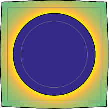
which is evaluated at the nodes of the background mesh, so that, in fact, only the interpolation $\phi^{h}\left(\mathchoice{\displaystyle\boldsymbol{x}}{\textstyle\boldsymbol{x}}{\scriptstyle\boldsymbol{x}}{\scriptscriptstyle\boldsymbol{x}}\right)$ is used. An example of an automatically generated mesh based on a background mesh with $6\times 6$ cubic elements is seen in Fig. 7(c). The exact solution is plotted in Fig. 7(d) in terms of the deformed configuration and the corresponding von Mises stress.

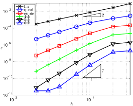
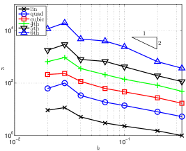
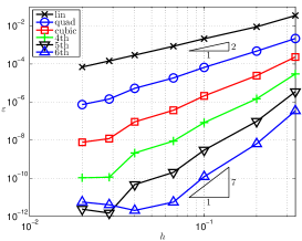
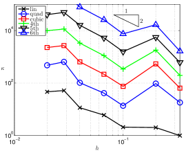
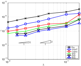
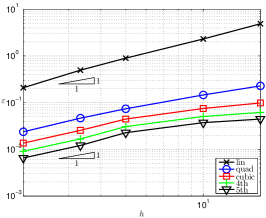
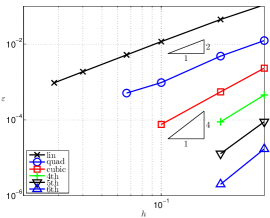
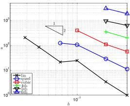
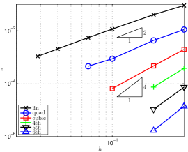
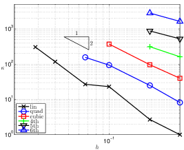
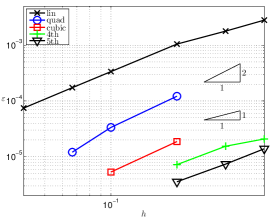
For the convergence study, the number of elements, $n_{d}$ , per dimensions of the background mesh is systematically increased and $n_{d}=\left\{6,10,20,30,50,70,100\right\}$ elements are used with varying orders between $1$ and $6$ . Results are shown in Fig. 8. In [21, 18], the focus is on the integration properties of the automatically generated meshes. Therefore, for example, the area of the mesh may be computed and compared to the exact area. For this example, this is shown in Fig. 8(a) and optimal convergence rates are achieved. In [22], also the interpolation error is studied, i.e., the ability to reproduce functions on the generated meshes. The error between a given example function and its interpolation is shown in Fig. 8(b) and is, again, optimal. It is clear that the ability to integrate and interpolate optimally is a necessary requirement for an optimal convergence in an approximation context as well. Convergence results of the approximated displacements in the $L_{2}$ -norm are shown in Figs. 8(c) and (d) based on background meshes composed by quadrilateral and triangular elements, respectively. The corresponding condition numbers $\kappa$ of the resulting system matrices for the different meshes are seen in Figs. 8(e) and (f).

6.2 Square shell with circular inclusion

A shell with the same geometry from above is considered, however, the void region is now filled with a different material. That is, the domain is again $\left[-1,1\right]\times\left[-1,1\right]$ and the interface is defined by the zero-level set of Eq. (6.1). In the outer region, Young’s modulus is $E_{1}=10$ and Poisson’s ratio $\nu_{1}=0.3$ . Inside the circular inclusion, there is $E_{2}=1$ and $\nu_{2}=0.25$ . An exact solution for this problem is found in [53, 19] and is given in the Appendix 8.2. The deformed configuration with von Mises stress is seen in Fig. 9(d). The corresponding displacements are prescribed at the outer boundary. For the convergence studies, the same background meshes with different numbers of elements per dimensions $n_{d}$ and element orders than in Section 6.1 are used. Examples for the generated conforming meshes based on background meshes with $n_{d}=\left\{6,10,20\right\}$ and cubic elements are seen in Fig. 9(a) to (c), respectively.

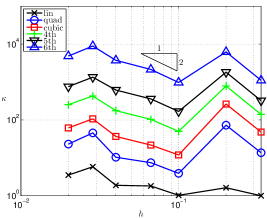
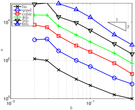
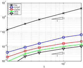
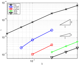
Convergence results are presented in Fig. 10. Integration and interpolation errors are no longer considered and the focus is only the approximation error of the displacements in the $L_{2}$ -norm. Figs. 10(a) and (b) show optimal convergence rates for background meshes composed by quadrilateral and triangular elements up to order $6$ , respectively. The corresponding condition numbers are shown in Figs. 10(c) and (d). It is seen that they are well-bounded, however, not as smooth as for manufactured meshes. Nevertheless, they behave with $O\left(h^{2}\right)$ as expected.

6.3 Cantilever beam

The next test cases in two dimensions serve the purpose to demonstrate the proposed higher-order CDFEM for more technical rather than academic setups. A cantilever beam with length $L=5.0\mathrm{m}$ and a variable thickness between $h=0.2\mathrm{m}$ and $0.4\mathrm{m}$ is considered first. The material is composed of steel with $E=2.1\cdot 10^{8}\,\nicefrac{\mathrm{kN}}{\mathrm{m^{2}}}$ and $\nu=0.3$ . The beam is loaded by gravity acting as a body force of $f_{y}=-78.5\,\nicefrac{\mathrm{kN}}{\mathrm{m^{3}}}$ and a vertical traction on the right side. This traction is distributed in a quadratic profile being zero at the upper and lower right side and reaching a maximum of $\sigma_{y}=-100\nicefrac{\mathrm{kN}}{\mathrm{m}}$ inbetween, leading to a force resultant of $F_{y}=-26.\bar{6}\,\mathrm{kN}$ .

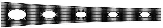
The beam features $5$ elliptical void regions. We place the $xy$ -coordinate system at the left side in the middle axis of the beam. $7$ level-set functions are used to define the geometry and the background meshes conform to the left and right side from the beginning. See Fig. 11(a) for the zero-level sets and an example background mesh. The $5$ elliptical void regions are defined from left to right as

\phi_{i}\left(\mathchoice{\displaystyle\boldsymbol{x}}{\textstyle\boldsymbol{x}}{\scriptstyle\boldsymbol{x}}{\scriptscriptstyle\boldsymbol{x}}\right)=a\cdot\left(x-x_{i}\right)^{2}+b\cdot y^{2}-R_{i}

with $a=\nicefrac{{1}}{{4}}$ , $b=\nicefrac{{3}}{{4}}$ , $x_{i}=\left\{1,3,5,7,9\right\}\cdot\nicefrac{{1}}{{2}}$ , and $R_{i}=\left\{22,12,8,6,6\right\}\cdot 10^{-3}$ . The $2$ level-set functions which define the upper and lower side of the beam are given as

\phi_{6}\left(\mathchoice{\displaystyle\boldsymbol{x}}{\textstyle\boldsymbol{x}}{\scriptstyle\boldsymbol{x}}{\scriptscriptstyle\boldsymbol{x}}\right)=g\left(x\right)-y,\,\phi_{7}\left(\mathchoice{\displaystyle\boldsymbol{x}}{\textstyle\boldsymbol{x}}{\scriptstyle\boldsymbol{x}}{\scriptscriptstyle\boldsymbol{x}}\right)=-g\left(x\right)-y\quad\text{with}\quad g\left(x\right)=\dfrac{x^{2}}{125}-\dfrac{2\cdot x}{25}+\dfrac{2}{5}.

None of these level-set functions has signed-distance property. Examples for automatically generated, conforming higher-order meshes for this test case are seen in Fig. 11(b) and (c).

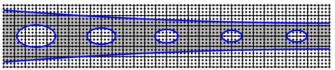
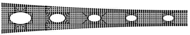
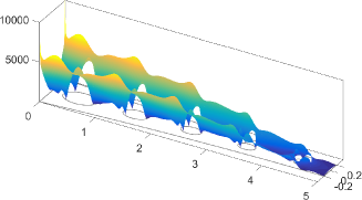
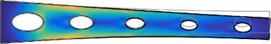
We consider two different support cases: In case 1, the left side of the beam is fully fixed. That is, zero-displacements are prescribed for the horizontal and vertical displacements at all nodes on the left. The deformed configuration is seen in Fig. 11(a) and the resulting von Mises stress in 3D view are shown in Fig. 11(b). It is seen that the stresses are singular at the upper and lower left corners, where the boundary conditions change from supported to free. This is well known in structural mechanics and will effect the convergence properties in a higher-order FEM as confirmed below. Support case 2 fixes all nodes on the boundary to the left elliptical void region. The resulting deformed configuration and von Mises stress are seen in Figs. 11(c) and (d). As seen, there are no singularities in the stresses for this support case and optimal convergence rates in the analysis are possible.

There are no analytical solutions available for the two different support scenarios of this test case, however, the stored energy has been computed by an overkill solution using standard $p$ -FEM. For support case 1, the elastic energy is $\mathfrak{e}=0.03246547385\pm 10^{-8}\mathrm{kNm}$ and for support case 2, $\mathfrak{e}=0.02361112384\pm 10^{-10}\mathrm{kNm}$ . The different uncertainties reflect the fact, that the singularities hinder an optimal convergence of the $p$ -FEM for support case 1 when computing the overkill solution.

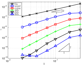
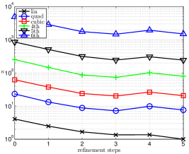
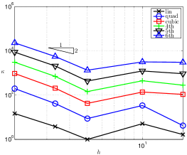
Convergence results are shown in Fig. 13. For the first support case where singularities are present, it is clearly seen from Fig. 13(a) that only first order convergence rates in the energy are achieved. It is nevertheless noted that from linear to cubic elements the results improve by about one order of magnitude. When comparing the results for even higher orders the improvements is more than two orders of magnitude. That is, although no higher-order convergence rates are achieved, there is still a significant improvement of the results. The energy error in Fig. 13(b) refers to the second support case and clearly converges with optimal rates as no singularities are present. The condition numbers for the different resolutions of the background meshes and various element orders are seen in Fig. 13(c). They are almost identical for the two support cases and behave as expected.

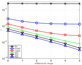
The focus is now only on support case 1 with the singularities at the upper and lower left corner of the beam. The results in Fig. 13 have been achieved without adaptive refinements at these singularities. Next, it is investigated how adaptive refinements improve the approximation error. The following results, presented in Fig. 14, are achieved for a background mesh with a fixed resolution but varying orders of the elements and a different number of refinement steps at the corners (up to $5$ ). The corresponding unrefined mesh taken as the starting mesh for each computation is seen in 11(c). Results are visualized in Fig. 14 where the horizontal axis shows the number of refinement steps. It is seen that for linear meshes, the adaptive refinements at the singularities does not change the results noticeably because the error in the bulk mesh is still dominant. However, for increasing orders of the elements, the local refinements improve the results to a great extent. So it is obvious that the singularities hinder optimal convergence rates for the higher-order elements as expected and that adaptivity is highly useful. For the $6th$ -order elements, the error is improved by $3$ orders of magnitude after $5$ refinements steps at the singularities!

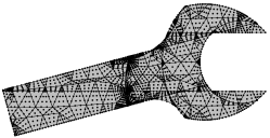
6.4 Spanner

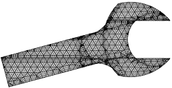
Next, the geometry shown in Fig. 15 is considered and refers to a spanner being very similar to normed spanner geometries defined in DIN 895. The geometry is embedded into a universal mesh composed by triangular elements of different orders. $11$ level-set functions are employed to define the geometry. There are $5$ straight lines defined by linear level-set functions

	$\displaystyle\phi_{i}\left(\mathchoice{\displaystyle\boldsymbol{x}}{\textstyle\boldsymbol{x}}{\scriptstyle\boldsymbol{x}}{\scriptscriptstyle\boldsymbol{x}}\right)$	$\displaystyle=$	$\displaystyle\mathchoice{\displaystyle\boldsymbol{n}}{\textstyle\boldsymbol{n}}{\scriptstyle\boldsymbol{n}}{\scriptscriptstyle\boldsymbol{n}}_{i}\cdot\left(\mathchoice{\displaystyle\boldsymbol{x}}{\textstyle\boldsymbol{x}}{\scriptstyle\boldsymbol{x}}{\scriptscriptstyle\boldsymbol{x}}-\mathchoice{\displaystyle\boldsymbol{x}}{\textstyle\boldsymbol{x}}{\scriptstyle\boldsymbol{x}}{\scriptscriptstyle\boldsymbol{x}}_{i}^{\star}\right),$
		$\displaystyle=$	$\displaystyle n_{x,i}\cdot\left(x-x_{i}^{\star}\right)+n_{y,i}\cdot\left(y-y_{i}^{\star}\right),$

which imply zero-level sets going through points $\mathchoice{\displaystyle\boldsymbol{x}}{\textstyle\boldsymbol{x}}{\scriptstyle\boldsymbol{x}}{\scriptscriptstyle\boldsymbol{x}}_{i}^{\star}$ with normal vectors $\mathchoice{\displaystyle\boldsymbol{n}}{\textstyle\boldsymbol{n}}{\scriptstyle\boldsymbol{n}}{\scriptscriptstyle\boldsymbol{n}}_{i}$ . See Table 1 for the concrete values of $\mathchoice{\displaystyle\boldsymbol{x}}{\textstyle\boldsymbol{x}}{\scriptstyle\boldsymbol{x}}{\scriptscriptstyle\boldsymbol{x}}_{i}^{\star}$ and $\mathchoice{\displaystyle\boldsymbol{n}}{\textstyle\boldsymbol{n}}{\scriptstyle\boldsymbol{n}}{\scriptscriptstyle\boldsymbol{n}}_{i}$ . All measurements for this test case are given in $\mathrm{mm}$ . Furthermore, there are a number of arc segments in the boundary definition of the spanner. Therefore, we need $6$ level-set functions,

	$\displaystyle\phi_{i}\left(\mathchoice{\displaystyle\boldsymbol{x}}{\textstyle\boldsymbol{x}}{\scriptstyle\boldsymbol{x}}{\scriptscriptstyle\boldsymbol{x}}\right)$	$\displaystyle=$	$\displaystyle\left\|\left\|\mathchoice{\displaystyle\boldsymbol{x}}{\textstyle\boldsymbol{x}}{\scriptstyle\boldsymbol{x}}{\scriptscriptstyle\boldsymbol{x}}-\mathchoice{\displaystyle\boldsymbol{x}}{\textstyle\boldsymbol{x}}{\scriptstyle\boldsymbol{x}}{\scriptscriptstyle\boldsymbol{x}}_{i}^{\circ}\right\|\right\|-R_{i}^{\circ},$
		$\displaystyle=$	$\displaystyle\sqrt{\left(x-x_{i}^{\circ}\right)^{2}+\left(y-y_{i}^{\circ}\right)^{2}}-R_{i}^{\circ},$

implying circular zero-level sets centered at $\mathchoice{\displaystyle\boldsymbol{x}}{\textstyle\boldsymbol{x}}{\scriptstyle\boldsymbol{x}}{\scriptscriptstyle\boldsymbol{x}}_{i}^{\circ}$ with radius $R_{i}^{\circ}$ . See Table 2 for the specific values of $\mathchoice{\displaystyle\boldsymbol{x}}{\textstyle\boldsymbol{x}}{\scriptstyle\boldsymbol{x}}{\scriptscriptstyle\boldsymbol{x}}_{i}^{\circ}$ and $R_{i}^{\circ}$ .

	$x_{i}^{\star}$	$y_{i}^{\star}$	$n_{x,i}$	$n_{y,i}$
mouth, top	$0.000000$	$30.000000$	$0.000000$	$1.000000$
mouth, bottom	$0.000000$	$-30.000000$	$0.000000$	$1.000000$
handle, up	$0.000000$	$36.100494$	$-0.258819$	$0.965926$
handle, bottom	$0.000000$	$-13.592762$	$-0.258819$	$0.965926$
handle, end	$0.000000$	$-929.486795$	$0.965926$	$0.258819$

Table 1: Definition of the straight segments of the spanner, measurements in

\mathrm{mm}

	$x_{i}^{\circ}$	$y_{i}^{\circ}$	$R_{i}^{\circ}$
circle 1	$0.000000$	$0.000000$	$42.000000$
circle 2	$0.000000$	$0.000000$	$80.000000$
circle 3	$-125.361456$	$66.697117$	$65.100000$
circle 4	$-90.856482$	$-81.419283$	$44.100000$
circle 5	$-37.000000$	$-21.000000$	$80.000000$
circle 6	$-37.000000$	$21.000000$	$80.000000$

Table 2: Definition of the arc segments of the spanner, measurements in

\mathrm{mm}

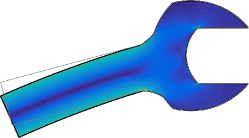
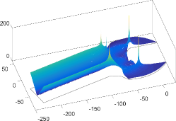
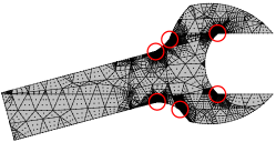
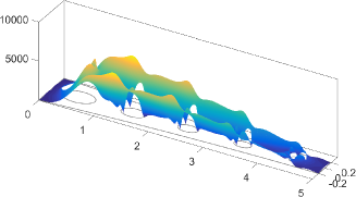
The material is again composed by steel with $E=2.1\cdot 10^{5}\,\nicefrac{\mathrm{N}}{\mathrm{mm^{2}}}$ and $\nu=0.3$ . The beam is loaded by gravity acting as a body force of $f_{y}=-78.5\cdot 10^{-6}\,\nicefrac{\mathrm{N}}{\mathrm{mm^{3}}}$ and a traction at the end of the handle. This traction acts in parallel direction of the handle and is distributed linearly between $-100\nicefrac{\mathrm{N}}{\mathrm{mm}}$ at the bottom side and $+100\nicefrac{\mathrm{N}}{\mathrm{mm}}$ on the top side. It loads the handle of the spanner with a resulting bending moment of $M_{z}=38400\,\mathrm{Nmm}$ . All nodes on the two straight, parallel sides of the mouth are fixed. The deformed configuration is shown in Fig. 15(b) scaled by a factor of $50$ . The geometry of the spanner features $6$ reentrant corners, two at the mouth, two on the top side between the handle and the front part and two on the opposite side, see the red circles in Fig. 15(f). It is thus clear that singular stresses have to be expected.

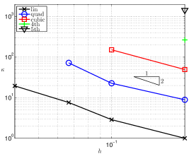
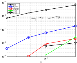
Convergence results are shown in Fig. 16. Again, there is no analytical solution available wherefore the stored energy is used for the convergence study. An overkill solution yields $\mathfrak{e}=61.49248\pm 10^{-4}\mathrm{Nmm}$ . Fig. 16(a) displays the convergence for automatically generated meshes without adaptive refinements at the singularities. Of course, only first order convergence rates are achieved due to the singularities, however, the error level is drastically improved for the higher-order meshes. Fig. 16(b) shows results for adaptively refined meshes as seen in Fig. 15(f). Only three refinement steps improve the error by about one order of magnitude for the higher-order elements. The only exception are linear elements where the error in the bulk mesh is still too large to improve much through a local refinement at the singularities only. Condition numbers are seen in Fig. 16(c) for the unrefined meshes and look quite similar for the refined case as well.

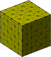
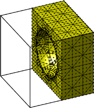
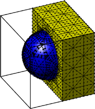
6.5 Cube with spherical hole

The next test cases feature three-dimensional geometries. The first case is the extension to three dimensions of the square shell with circular hole from Section 6.1 and the same material properties are used here. The domain is $\left[-1,1\right]^{3}$ with a spherical hole of radius $R=0.7123$ , see Fig. 17(a) for a sketch of the situation. An example background mesh is seen in Fig. 17(b) and a resulting conforming mesh with hole in (c). The deformed configuration according to the exact solution from [24], see the Appendix 8.3, is displayed in Fig. 17(d).

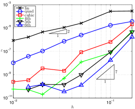
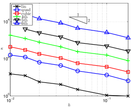
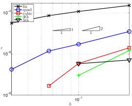
For the convergence study, the number of elements per dimensions, $n_{d}$ , of the background mesh is systematically increased and $n_{d}=\left\{6,10,20,30,50,70\right\}$ elements are used with varying orders between $1$ and $6$ . Only meshes with less than $500.000$ nodes are considered, leading to $1.5\cdot 10^{6}$ degrees of freedom as three displacement components at each node are present. Convergence results of the aproximation error are displayed in Fig. 18(a) and are optimal as expected. Note that in [21, 18], integration errors for this test case are investigated and in [22], interpolation errors. Nevertheless, these are the first higher-order convergence results of approximation errors achieved with the CDFEM in three dimensions reported so far. Fig. 18(b) shows the corresponding condition numbers which are well-bounded and prove the success of the node manipulations discussed in Section 4.

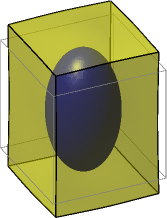
6.6 Cube with spherical inclusion

This test case is the extension of the square shell with circular inclusion from Section 6.2 to three dimensions. Fig. 19(a) shows an example for a resulting conforming mesh and elements inside the sphere are plotted in blue. The exact solution is found in [24] and also repeated in the Appendix 8.4. The corresponding deformed configuration is seen in Fig. 19(b). The convergence study is along the lines of Section 6.5 and results are displayed in Fig. 18. Again, the convergence rates are optimal and condition numbers behave as expected.

6.7 Bi-material gyroid

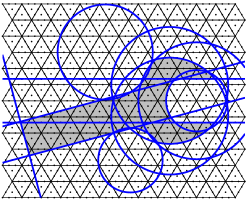
Another example of a domain in $\left[-1,1\right]^{3}$ composed by two different materials is considered next where the materials are seperated by the so-called “gyroid” surface, implied by the zero-level set of

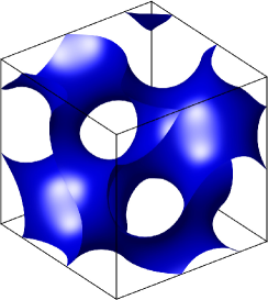
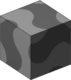
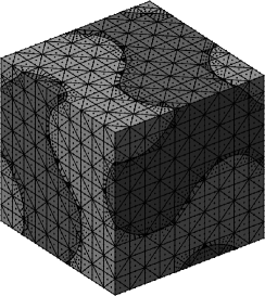
\phi\left(\mathchoice{\displaystyle\boldsymbol{x}}{\textstyle\boldsymbol{x}}{\scriptstyle\boldsymbol{x}}{\scriptscriptstyle\boldsymbol{x}}\right)=\sin x^{\star}\cdot\cos z^{\star}+\sin y^{\star}\cdot\cos x^{\star}+\sin z^{\star}\cdot\cos y^{\star}

with $x^{\star}=\pi\cdot\left(x+q\right)$ , $y^{\star}=\pi\cdot\left(y+q\right)$ , $z^{\star}=\pi\cdot\left(z+q\right)$ with $q=0.123456$ . See Fig. 21(a) and (b) for a representation of the zero-isosurface and the resulting domain. Fig. 21(c) shows an example of an automatically generated mesh of order $3$ . The same material parameters as in Section 6.2 are chosen. All displacements on the boundaries are fixed and the domain is loaded by a body force of $f_{z}=-1$ in vertical direction.

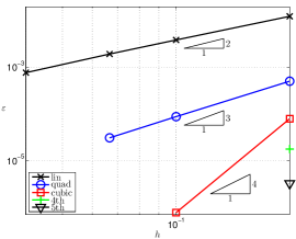
For the convergence studies, background meshes with $\{10,20,30,50\}$ elements per dimensions are chosen unless they lead to more than $10^{6}$ degrees of freedom. For this rather complex zero-level set, coarser meshes with $<10$ elements per dimension lead to a significant number of adaptive refinements, so that the element lengths $h$ vary too much to obtain representative values for the convergence plots. Fig. 22(a) shows the convergence rates in the same style than before, however, the limitation on the number of degrees of freedom leads to less data points. Therefore, Fig. 22(b) shows convergence results on meshes with $10$ elements per dimension only but with different element orders. The error is plotted with respect to the degrees of freedom and expontential convergence is obtained. Finally, the condition number is seen in Fig. 22(c) and is bounded as expected.

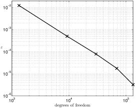
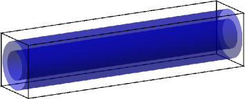
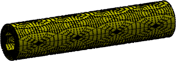
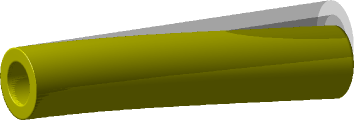
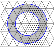
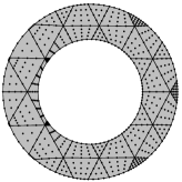
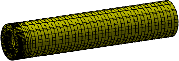
6.8 Cantilever tube

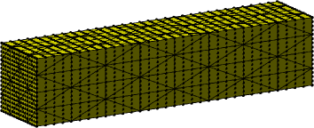
The next test case is more technical. We consider a pipe of length $L=5\mathrm{m}$ with an inner radius $r_{\mathrm{i}}=0.3\mathrm{m}$ and an outer radius $r_{\mathrm{o}}=0.5\mathrm{m}$ . The pipe is clamped on one side, i.e., all displacement components are enforced to vanish there. The material is composed by steel with $E=2.1\cdot 10^{8}\,\nicefrac{\mathrm{kN}}{\mathrm{m^{2}}}$ and $\nu=0.3$ . The beam is loaded by gravity acting as a body force of $f_{z}=-78.5\,\nicefrac{\mathrm{kN}}{\mathrm{m^{3}}}$ . The background mesh is given in $\Omega_{\mathrm{BG}}=\left[0,5\right]\times\left[-0.55,0.55\right]^{2}$ and the pipe walls are implied by the two level-set functions

\phi_{\mathrm{i/o}}=\sqrt{y^{2}+z^{2}}-r_{\mathrm{i/o}},

see Fig. 23(a). An example background mesh is seen in Fig. 23(b) and the resulting conforming mesh in Fig. 23(c). The deformed configuration scaled by a factor of $1000$ is shown in Fig. 23(d). It is also useful to generate a mesh for the pipe by first generating a conforming 2D mesh of the cross-sectional area based on a 2D background mesh as shown in Figs. 24(a) and (b) and then extruding this in $x$ -direction generating prismatic and hexahedral elements. This also allows for an efficient refinement near the clamped side, see e.g., Fig. 24(c).

The situation is comparable to a clamped Bernoulli beam governed by the differential equation $EI\cdot w(x)^{\prime\prime\prime\prime}=q(x)$ with the second moment of area $I=\nicefrac{{\pi}}{{4}}\cdot\left(r_{\mathrm{o}}^{4}-r_{\mathrm{i}}^{4}\right)$ , the line load $q(x)=-f_{z}\cdot A$ and the sectional area $A=\pi\cdot\left(r_{\mathrm{o}}^{2}-r_{\mathrm{i}}^{2}\right)$ . The line load $q$ and the deflection $w$ are positive in downward direction, i.e., $w=-u_{z}$ . With the left side ( $x=0$ ) clamped and the right side ( $x=L$ ) fully free, the analytical solution for the bending curve is

w(x)=\dfrac{q}{EI}\cdot\left(\dfrac{L^{2}}{4}x^{2}-\dfrac{L}{6}x^{3}+\dfrac{1}{24}x^{4}\right).

This yields a deflection on the right side of $w\left(L\right)=\frac{qL^{4}}{8EI}=0.343575\mathrm{mm}$ and a stored energy of $\mathfrak{e}=\nicefrac{{1}}{{2}}\int M\left(x\right)\cdot\varkappa\left(x\right)\,dx=\frac{EI}{2}\int\left[w^{\prime\prime}\left(x\right)\right]^{2}\,dx=\frac{q^{2}L^{5}}{40EI}\approx 0.013557\mathrm{kNm}$ . An overkill FEM-solution of the three-dimensional problem yields $\max\left(\left|u_{z}\right|\right)=0.3605575\pm 10^{-6}\mathrm{mm}$ and $\mathfrak{e}=0.01473635\mathrm{\pm 10^{-7}kNm}$ which is quite similar and taken for the convergence studies.

Results are seen in Fig. 25(a) and (b) for meshes generated from 3D background meshes as in Fig. 23(b), and in Fig. 25(c) and (d) for meshes generated from extruding 2D meshes as shown in Fig. 24. The convergence rates are sub-optimal as expected due to the singularties in the stresses at the clamped side. Nevertheless, it is seen that higher-order elements are able to significantly improve the results. Obviously, the refinement on the clamped side as for the extruded meshes further improves the results.

7 Conclusions

A higher-order CDFEM is proposed which automatically generates higher-order, conforming meshes based on background meshes and level-set data. The decomposition of cut elements into conforming sub-elements has been described before, e.g., in [21, 18, 22] in the context of integration and interpolation. Herein, this idea is extended to the approximation of BVPs. In addition to the fact that the sub-elements must conform to the zero-level sets, this involves the following additional challenges: The element set must be continuous accross element boundaries so that hanging nodes are avoided. Therefore, an adaptive procedure which guarantees the regularity of the background mesh is suggested. Furthermore, the generated elements must be shape-regular wherefore a node manipulation is proposed which (slightly) moves nodes near the zero-level sets to guarantee bounded ratios of the areas/volumes on the two sides of the cut elements. A suitable finite element mesh composed by higher-order elements may then be generated from the element set, i.e., the connectivity information is set up.

In particular, the combination of the automatic mesh generation and adaptive refinements, not only for elements where the decomposition fails, but also where a more accurate geometry description or approximation of the BVP is desired, is found to be a key ingredient of the proposed method. Numerical results are presented in the context of linear elasticity without loss of generality of the method. Elements up to order $6$ are investigated herein and higher-order convergence rates are achieved.

The resulting method is stable, efficent and achieves optimal, higher-order convergence rates in two and three dimensions. As such, it is an attractive alternative to FDMs and the XFEM. Remaining challenges include moving interfaces and iterative solvers. In a forthcoming part of this series of publications, we shall report on a higher-order FDM where the shape functions of the background mesh are used for the approximation and comparisons to the CDFEM discussed herein will be made.

8 Appendix

8.1 Exact solution for the square shell with circular hole

The exact solution for this problem of an infinite plate with a traction-free circular hole under uniaxial tension with $\sigma_{0}$ is, e.g., found in [54, 30]. It is given in polar coordinates $\left(r,\theta\right)$ as

	$\displaystyle u_{x}\left(r,\theta\right)$	$\displaystyle=$	$\displaystyle\sigma_{0}\cdot\frac{R}{8\mu}\left[\frac{r}{R}\left(\varkappa+1\right)\cos\theta+\frac{2R}{r}\left(\left(1+\varkappa\right)\cos\theta+\cos 3\theta\right)-\frac{2R^{3}}{r^{3}}\cos 3\theta\right],$
	$\displaystyle u_{y}\left(r,\theta\right)$	$\displaystyle=$	$\displaystyle\sigma_{0}\cdot\frac{R}{8\mu}\left[\frac{r}{R}\left(\varkappa-3\right)\sin\theta+\frac{2R}{r}\left(\left(1-\varkappa\right)\sin\theta+\sin 3\theta\right)-\frac{2R^{3}}{r^{3}}\sin 3\theta\right],$

where $R$ is the radius of the hole and $\varkappa$ is the Kolosov constant defined as

\varkappa=\begin{cases}3-4\nu&\quad\text{for plane strain},\\ \dfrac{3-\nu}{1+\nu}&\quad\text{for plane stress}.\end{cases}

8.2 Exact solution for the square shell with circular inclusion

The exact solution for this test case is given, e.g., in [53, 19, 17]. The radius of the inclusion is $a=R$ and another scalar value $b>a$ defines a radius where a given traction is applied. The displacements in direction of the polar coordinates are

	$\displaystyle u_{r}\left(r,\theta\right)$	$\displaystyle=$	$\displaystyle\left\{\begin{array}[]{cl}\left((1-\frac{b^{2}}{a^{2}})\alpha+\frac{b^{2}}{a^{2}}\right)\cdot r,&\quad 0\leq r\leq a,\\ \left((1-\frac{b^{2}}{r^{2}})\alpha+\frac{b^{2}}{r^{2}}\right)\cdot r,&\quad a<r\leq b,\end{array}\right.$		(8.3)
	$\displaystyle u_{\theta}\left(r,\theta\right)$	$\displaystyle=$	$\displaystyle 0.$		(8.4)

The parameter $\alpha$ involved in these definitions is

\alpha=\frac{\left(\lambda_{1}+\mu_{1}+\mu_{2}\right)b^{2}}{\left(\lambda_{2}+\mu_{2}\right)a^{2}+\left(\lambda_{1}+\mu_{1}\right)\left(b^{2}-a^{2}\right)+\mu_{2}b^{2}}.

(8.5)

It is trivial to transform these displacements into $x$ - and $y$ -direction using the transformation matrix $T$ , hence,

\left[\begin{array}[]{c}u_{x}\\ u_{y}\end{array}\right]=\left[\begin{array}[]{cc}\cos\theta&-\sin\theta\\ \sin\theta&\cos\theta\end{array}\right]\cdot\left[\begin{array}[]{c}u_{r}\\ u_{\theta}\end{array}\right].

8.3 Exact solution for the cube with spherical hole

The solution is defined in spherical coordinates $\left(r,\theta,\varphi\right)$ related to the Cartesian coordinates $\left(x,y,z\right)$ by

r=\sqrt{x^{2}+y^{2}+z^{2}},\quad\tan\theta=\nicefrac{{y}}{{x}},\quad\cos\varphi=\nicefrac{{z}}{{r}},

with $0\leq\theta\leq 2\pi$ and $0\leq\varphi\leq\pi$ . Let $T$ be the tension in direction $\theta=0$ acting as a load. Then, the solution for a cavity with radius $R$ is given in spherical displacement components as follows [24]:

$\displaystyle u_{r}$	$\displaystyle=$	$\displaystyle u_{r}^{0}-\dfrac{A}{r^{2}}-\dfrac{3B}{r^{4}}+\left(\dfrac{5-4\nu}{1-2\nu}\cdot\dfrac{C}{r^{2}}-\dfrac{9B}{r^{4}}\right)\cos\left(2\theta\right),$	(8.6)
$\displaystyle u_{\theta}$	$\displaystyle=$	$\displaystyle u_{\theta}^{0}-\left(\dfrac{2C}{r^{2}}+\dfrac{6B}{r^{4}}\right)\sin\left(2\theta\right),$	(8.7)
$\displaystyle u_{\varphi}$	$\displaystyle=$	$\displaystyle 0,$

with

	$\displaystyle u_{r}^{0}$	$\displaystyle=$	$\displaystyle\dfrac{Tr}{2E}\left[\left(1-\nu\right)+\left(1+\nu\right)\cos\left(2\theta\right)\right],$		(8.8)
	$\displaystyle u_{\theta}^{0}$	$\displaystyle=$	$\displaystyle-\dfrac{Tr}{2E}\left(1+\nu\right)\sin\left(2\theta\right),$		(8.9)

and the coefficients

\displaystyle A=-\dfrac{R^{3}T}{8\mu}\cdot\dfrac{13-10\nu}{7-5\nu},

\displaystyle\quad B=\dfrac{R^{5}T}{8\mu}\cdot\dfrac{1}{7-5\nu},

\displaystyle\quad C=\dfrac{R^{3}T}{8\mu}\cdot\dfrac{5\left(1-2\nu\right)}{7-5\nu}.

This is easily converted to Cartesian coordinates based on the transformation matrix $\mathchoice{\displaystyle\mathbf{T}}{\textstyle\mathbf{T}}{\scriptstyle\mathbf{T}}{\scriptscriptstyle\mathbf{T}}$ ,

\left[\begin{array}[]{c}u_{x}\\ u_{y}\\ u_{z}\end{array}\right]=\mathchoice{\displaystyle\mathbf{T}}{\textstyle\mathbf{T}}{\scriptstyle\mathbf{T}}{\scriptscriptstyle\mathbf{T}}\cdot\left[\begin{array}[]{c}u_{r}\\ u_{\theta}\\ u_{\varphi}\end{array}\right]\qquad\mathrm{with}\;\mathchoice{\displaystyle\mathbf{T}}{\textstyle\mathbf{T}}{\scriptstyle\mathbf{T}}{\scriptscriptstyle\mathbf{T}}=\left[\begin{array}[]{ccc}\sin\theta\cos\varphi&\cos\theta\cos\varphi&-\sin\varphi\\ \sin\theta\sin\varphi&\cos\theta\sin\varphi&\cos\varphi\\ \cos\theta&-\sin\theta&0\end{array}\right].

8.4 Exact solution for the cube with spherical inclusion

The exact solution in spherical displacements for the spherical inclusion problem of Section 6.6 is given as [24]

$\displaystyle u_{r}$	$\displaystyle=$	$\displaystyle\begin{cases}Hr+Fr+3Fr\cdot\cos\left(2\theta\right)&\mathrm{for}\;r\leq R\\ u_{r}^{0}-\dfrac{A}{r^{2}}-\dfrac{3B}{r^{4}}+\left(\dfrac{5-4\nu_{1}}{1-2\nu_{1}}\cdot\dfrac{C}{r^{2}}-\dfrac{9B}{r^{4}}\right)\cos\left(2\theta\right)&\mathrm{for}\;r>R\end{cases}$
$\displaystyle u_{\theta}$	$\displaystyle=$	$\displaystyle\begin{cases}-3Fr\cdot\sin\left(2\theta\right)&\mathrm{for}\;r\leq R\\ u_{\theta}^{0}-\left(\dfrac{2C}{r^{2}}+\dfrac{6B}{r^{4}}\right)\sin\left(2\theta\right)&\mathrm{for}\;r>R\end{cases}$
$\displaystyle u_{\varphi}$	$\displaystyle=$	$\displaystyle 0$

References

- [1] Abedian, A.; Parvizian, J.; Düster, A.; Khademyzadeh, H.; Rank, E.: Performance of different integration schemes in facing discontinuities in the Finite Cell Method. International Journal of Computational Methods, 10, 1 – 24, 2013.
- [2] Abedian, A.; Parvizian, J.; Düster, A.; Rank, E.: The finite cell method for the flow theory of plasticity. Finite Elem. Anal. Des., 69, 37 – 47, 2013.
- [3] Ainsworth, M.; Senior, B.: Aspects of an adaptive -finite element method: Adaptive strategy, conforming approximation and efficient solvers. Comp. Methods Appl. Mech. Engrg., 150, 65 – 87, 1997.
- [4] Babuška, I.; Caloz, G.; Osborn, J.E.: Special finite element methods for a class of second order elliptic problems with rough coefficients. SIAM J. Numer. Anal., 31, 945 – 981, 1994.
- [5] Babuška, I.; Melenk, J.M.: The partition of unity method. Internat. J. Numer. Methods Engrg., 40, 727 – 758, 1997.
- [6] Bathe, K.J.: Finite Element Procedures. Prentice-Hall, Englewood Cliffs, NJ, 1996.
- [7] Belytschko, T.; Black, T.: Elastic crack growth in finite elements with minimal remeshing. Internat. J. Numer. Methods Engrg., 45, 601 – 620, 1999.
- [8] Belytschko, T.; Liu, W.K.; Moran, B.: Nonlinear Finite Elements for Continua and Structures. John Wiley & Sons, Chichester, 2000.
- [9] Burman, E.; Claus, S.; Hansbo, P.; Larson, M.G.; Massing, A.: CutFEM: Discretizing geometry and partial differential equations. Internat. J. Numer. Methods Engrg., 104, 472 – 501, 2015.
- [10] Burman, E.; Hansbo, P.: Fictitious domain finite element methods using cut elements: I. A stabilized Lagrange multiplier method. Comp. Methods Appl. Mech. Engrg., 199, 2680 – 2686, 2010.
- [11] Burman, E.; Hansbo, P.: Fictitious domain finite element methods using cut elements: II. A stabilized Nitsche method. Applied Numerical Mathematics, 62, 328 – 341, 2012.
- [12] Cheng, K.W.; Fries, T.P.: Higher-order XFEM for curved strong and weak discontinuities. Internat. J. Numer. Methods Engrg., 82, 564 – 590, 2010.
- [13] Demkowicz, L.: Computing with -adaptive finite elements. Vol. 1: One- and two-dimensional elliptic and Maxwell problems. Chapman & Hall/CRC Applied Mathematics and Nonlinear Science Series, Boca Raton, FL, 2007.
- [14] Deuflhard, P.; Weiser, M.: Adaptive numerical solutions of PDEs. De Gruyter, Berlin, 2012.
- [15] Dréau, K.; Chevaugeon, N.; Moës, N.: Studied X-FEM enrichment to handle material interfaces with higher order finite element. Comp. Methods Appl. Mech. Engrg., 199, 1922 – 1936, 2010.
- [16] Düster, A.; J. Parvizian, Z. Yang; Rank, E.: The finite cell method for three-dimensional problems of solid mechanics. Comp. Methods Appl. Mech. Engrg., 197, 3768 – 3782, 2008.
- [17] Fries, T.P.: A corrected XFEM approximation without problems in blending elements. Internat. J. Numer. Methods Engrg., 75, 503 – 532, 2008.
- [18] Fries, T.P.: Higher-order accurate integration for cut elements with Chen-Babuška nodes. In Advances in Discretization Methods: Discontinuities, virtual elements, fictitious domain methods. (Ventura, G.; Benvenuti, E., Eds.), Vol. 12, SEMA SIMAI Springer Series, Springer, Berlin, 245 – 269, 2016.
- [19] Fries, T.P.; Belytschko, T.: The Intrinsic XFEM: A Method for Arbitrary Discontinuities without Additional Unknowns. Internat. J. Numer. Methods Engrg., 68, 1358 – 1385, 2006.
- [20] Fries, T.P.; Belytschko, T.: The extended/generalized finite element method: An overview of the method and its applications. Internat. J. Numer. Methods Engrg., 84, 253 – 304, 2010.
- [21] Fries, T.P.; Omerović, S.: Higher-order accurate integration of implicit geometries. Internat. J. Numer. Methods Engrg., 106, 323 – 371, 2016.
- [22] Fries, T.P.; Omerović, S.; Schöllhammer, D.; Steidl, J.: Higher-order meshing of implicit geometries—part I: Integration and interpolation in cut elements. Comp. Methods Appl. Mech. Engrg., 313, 759 – 784, 2017.
- [23] Fries, T.P.; Schöllhammer, D.: Higher-order meshing of implicit geometries—part II: Approximations on manifolds. Comp. Methods Appl. Mech. Engrg., 0, submitted, 2017.
- [24] Goodier, J.N.: Concentration of stress around spherical and cylindrical inclusions and flaws. J. Appl. Mech., ASME, 55, 39 – 44, 1933.
- [25] Hansbo, A.; Hansbo, P.: An unfitted finite element method, based on Nitsche’s method, for elliptic interface problems. Comp. Methods Appl. Mech. Engrg., 191, 5537 – 5552, 2002.
- [26] Hughes, T.J.R.; Cottrell, J.A.; Bazilevs, Y.: Isogeometric analysis: CAD, finite elements, NURBS, exact geometry, and mesh refinement. Comp. Methods Appl. Mech. Engrg., 194, 4135 – 4195, 2005.
- [27] Kramer, R.M.J.; Noble, D.R.: An effective strategy for improving the quality of conformal mesh decompositions on unstructured simplex meshes. Internat. J. Numer. Methods Engrg., 0, submitted, 2017.
- [28] Legay, A.; Wang, H.W.; Belytschko, T.: Strong and weak arbitrary discontinuities in spectral finite elements. Internat. J. Numer. Methods Engrg., 64, 991 – 1008, 2005.
- [29] Leveque, R.; Randall, J.; Li, Z.: Immersed interface method for elliptic equations with discontinuous coefficients and singular sources. SIAM J. Numer. Anal., 31, 1019 – 1044, 1994.
- [30] Liu, G.R.: Meshless Methods. CRC Press, Boca Raton, 2002.
- [31] Loehnert, S.: A stabilization technique for the regularization of nearly singular extended finite elements. Comput. Mech., 54, 523 – 533, 2014.
- [32] Löhner, R.; Cebral, J.R.; Camelli, F.F.; Baum, J.D.; Mestreau, E.L.; Soto, O.A.: Adaptive embedded/immersed unstructured grid techniques. Archives Of Computational Methods In Engineering, 14, 279 – 301, 2007.
- [33] Marussig, B.; Zechner, J.; Beer, G.; Fries, T.P.: Fast isogeometric boundary element method based on independent field approximation. Comp. Methods Appl. Mech. Engrg., 284, 458 – 488, 2015.
- [34] Melenk, J.M.; Babuška, I.: The partition of unity finite element method: basic theory and applications. Comp. Methods Appl. Mech. Engrg., 139, 289 – 314, 1996.
- [35] Moës, N.; Dolbow, J.; Belytschko, T.: A finite element method for crack growth without remeshing. Internat. J. Numer. Methods Engrg., 46, 131 – 150, 1999.
- [36] Morton, D.J.; Tyler, J.M.; Dorroh, J.R.: A new 3d finite element for adaptive -refinement in 1-irregular meshes. Internat. J. Numer. Methods Engrg., 38, 3989 – 4008, 1995.
- [37] Moumnassi, M.; Belouettar, S.; Béchet, É.; Bordas, S.P.A.; Quoirin, D.; Potier-Ferry, M.: Finite element analysis on implicitly defined domains: An accurate representation based on arbitrary parametric surfaces. Comp. Methods Appl. Mech. Engrg., 200, 774 – 796, 2011.
- [38] Neittaanmäki, P.; Tiba, D.: An embedding of domains approach in free boundary problems and optimal design. SIAM J. Control Optim., 33, 1587 – 1602, 1995.
- [39] Noble, D.R.; Newren, E.P.; Lechman, J.B.: A conformal decomposition finite element method for modeling stationary fluid interface problems. Int. J. Numer. Methods Fluids, 63, 725 – 742, 2010.
- [40] Omerović, S.; Fries, T.P.: Conformal higher-order remeshing schemes for implicitly defined interface problems. Internat. J. Numer. Methods Engrg., 109, 763 – 789, 2017.
- [41] Osher, S.; Fedkiw, R.P.: Level set methods: an overview and some recent results. J. Comput. Phys., 169, 463 – 502, 2001.
- [42] Osher, S.; Fedkiw, R.P.: Level Set Methods and Dynamic Implicit Surfaces. Springer, Berlin, 2003.
- [43] Parvizian, J.; Düster, A.; Rank, E.: Finite cell method: h- and p-extension for embedded domain problems in solid mechanics. Comput. Mech., 41, 121 – 133, 2007.
- [44] Rangarajan, R.; Lew, A.J.: Universal Meshes: A new paradigm for computing with nonconforming triangulations. arxiv:1201.4903, 2012.
- [45] Saiki, E.M.; Biringen, S.: Numerical Simulation of a Cylinder in Uniform Flow: Application of a Virtual Boundary Method. J. Comput. Phys., 123, 450 – 465, 1996.
- [46] Schillinger, D.; Düster, A.; Rank, E.: The --adaptive finite cell method for geometrically nonlinear problems of solid mechanics. Internat. J. Numer. Methods Engrg., 89, 1171 – 1202, 2012.
- [47] Schillinger, D.; Ruess, M.: The Finite Cell Method: A Review in the Context of Higher-Order Structural Analysis of CAD and Image-Based Geometric Models. Archive Comp. Mech. Engrg., 22, 391 – 455, 2015.
- [48] Sethian, J.A.: Level Set Methods and Fast Marching Methods. Cambridge University Press, Cambridge, 2 edition, 1999.
- [49] Šolín, P.; Červený, J.; Doležel, I.: Arbitrary-level hanging nodes and automatic adaptivity in the -FEM. Math. Comput. Simul., 77, 117 – 132, 2008.
- [50] Šolín, P.; Segeth, K.; Doležel, I.: Higher-order finite element methods. CRC Press, Boca Raton, FL, 2003.
- [51] Strouboulis, T.; Babuška, I.; Copps, K.: The design and analysis of the generalized finite element method. Comp. Methods Appl. Mech. Engrg., 181, 43 – 69, 2000.
- [52] Strouboulis, T.; Copps, K.; Babuška, I.: The generalized finite element method: an example of its implementation and illustration of its performance. Internat. J. Numer. Methods Engrg., 47, 1401 – 1417, 2000.
- [53] Sukumar, N.; Chopp, D.L.; Moës, N.; Belytschko, T.: Modeling holes and inclusions by level sets in the extended finite-element method. Comp. Methods Appl. Mech. Engrg., 190, 6183 – 6200, 2001.
- [54] Szabó, B.; Babuška, I.: Finite Element Analysis. John Wiley & Sons, Chichester, 1991.
- [55] Szabó, B.; Düster, A.; Rank, E.: The p-Version of the Finite Element Method, Chapter 5, 119 – 139. John Wiley & Sons, Chichester, 2004.
- [56] Uzgoren, E.; J. Sim, J.; Shyy, W.: Marker-based, 3-D adaptive Cartesian grid method for multiphase flow around irregular geometries. Comput. Phys. Comm., 5, 1 – 41, 2009.
- [57] Ye, T.; Mittal, R.; Udaykumar, H.S.; Shyy, W.: An Accurate Cartesian Grid Method for Viscous Incompressible Flows with Complex Immersed Boundaries. J. Comput. Phys., 156, 209 – 240, 1999.
- [58] Zienkiewicz, O.C.; Taylor, R.L.: The Finite Element Method, Vol. 1 – 3. Butterworth-Heinemann, Oxford, 2000.